1. Introduction
Rice is one of the world’s three major food crops and a primary food source for over half the global population. China boasts a cultivation area of approximately 29.92 million hectares, ranking first in the world in terms of annual rice production. Plant height is a comprehensive reflection of the intrinsic characteristics of rice plants, as well as environmental factors such as climate, hydrology, and soil, and is an important basis for monitoring growth, estimating yield, and evaluating greenhouse gas emissions [
1]. Therefore, the accurate and timely acquisition of rice plant height across extensive areas is of great significance for safeguarding national food security, promoting the reduction of agricultural emissions and efficiency enhancement, advancing carbon sequestration, and contributing to the development of a national dual carbon strategy.
The conventional approach for determining rice height primarily relies on field observations, which are time-consuming and labor-intensive processes with limited coverage and inadequate timelines. Remote sensing technology is an important means of Earth observation and offers advantages such as large-scale synchronous observation, short revisit periods, and a high level of timeliness. Furthermore, it is already widely utilized for crop monitoring and parameter acquisition. Rice is frequently grown in hot and humid environments that experience cloudy and rainy weather during the growing season, and this results in challenges regarding optical remote sensing data acquisition [
2,
3]. Synthetic aperture radar (SAR) can uniquely penetrate clouds, allowing for observations under most weather conditions. This is advantageous for the inversion of rice parameters in cloudy and rainy weather during the growing season [
4,
5].
The main methods for SAR vegetation height monitoring are based on radiative transfer modeling, Interferometric Synthetic Aperture Radar (InSAR)-based Digital Elevation Model (DEM) differencing, Polarimetric Synthetic Aperture Radar Interferometry (PolInSAR)-based complex coherence differencing, and model-solving algorithms [
6,
7]. The method based on radiative transfer theory uses the radiative transfer equation to model the quantitative relationship between radar backscattering coefficients and plant structure (plant height), dielectric properties, and thus plant height inversion [
8]. The advantage of this method lies in its solid physical foundation; however, it suffers from the drawback of having a plethora of model parameters, resulting in lower computational accuracy. The InSAR-based DEM difference method obtains phase difference information from two or more images of different orbits, calculates the digital surface model (DSM), and obtains the vegetation height by differentiating the DSM from the external DEM data. The accuracy of this method is affected by the heterogeneity of the vegetation as well as the accuracy of the external DEM [
9,
10]. PolInSAR combines the characteristics of polarimetric SAR, which is sensitive to the shape and direction of scatterers, and the characteristics of InSAR, which is sensitive to the spatial distribution of scatterers [
11]. Furthermore, it establishes a quantitative relationship for the multi-polarized phase interference using a multichannel polarization synthesis technique, which can significantly improve the signal-to-noise ratio of the interferometric phase and improve the accuracy of the inversion of the ground height and parameters [
12,
13,
14]. The PolInSAR complex coherence difference method relies on the phase differences associated with different scattering mechanisms to estimate vegetation height. However, the reliability of this method is limited by the penetration depth of the microwave signals. Real surface information cannot be obtained when the penetration depth is shallow [
15]. The PolInSAR model-based inversion approach abstracts vegetated scenes into two layers: vegetation and ground. This replaces complex vegetation structure functions with empirical models containing a limited number of unknown parameters, thereby simplifying the structural functions. Model-based inversion methods are computationally efficient and can produce higher levels of inversion accuracy. Among these, the random volume over ground (RVoG) and oriented volume over ground (OVoG) models are the most widely applied for PolInSAR vegetation height retrieval [
16,
17,
18]. Many studies on agricultural vegetation suggest that the orientation effects introduced by stalk shape may result in polarization-dependent propagation through the canopy [
19]. In such cases, considering the propagation direction makes the OVoG model more suitable for simulating crop height. The main constraint of using such a model is the large number of structural parameters with respect to the available measurements. Solving the numerous parameters of the OVoG model using a single baseline often leads to ill-conditioned solutions. Therefore, the utilization of prior knowledge assumptions or the extension of the observation space dimension via multi-baseline data is required.
Currently, PolInSAR vegetation height inversion primarily uses satellite-based SAR, airborne SAR, and microwave anechoic chamber data. Spaceborne SAR data from satellites such as Sentinel-1, GF-3, and TanDEM/TerraSAR-X can also be utilized to provide the PolInSAR data. However, these satellites have rarely incorporated PolInSAR crop monitoring into their design and operation and are typically utilized to assess forest height inversion. Consequently, there is a scarcity of baseline data that are specifically sensitive to crop structure. Noelia et al. [
18] present a modified PolInSAR inversion methodology based on the operator TrCoh and validated it with reference data obtained from TanDEM-X data in the Spanish rice zone, and the root mean square error of the improved method was improved by 7 cm compared to the traditional method. Lopez Sanchez et al. [
20] inverted rice heights in Spain and Turkey using time-series large baseline PolInSAR data taken by TanDEM-X from April to September 2015, with a root mean square error (RMSE) in the range of 10–20 cm; however, the estimates were distorted since the initial rice growth heights were <40 cm owing to the low sensitivity for short plants when using PolInSAR data. Airborne SAR data offers a higher resolution than Spaceborne SAR data and can provide data with various baselines and incidence angles. Notable platforms include E-SAR (Germany), F-SAR (Germany), UAVSAR (USA), and RAMSES (France) [
21]. Lopez-Sanchez et al. inverted the heights of crops such as oilseed rape, maize, wheat, barley, and sugar beet based on the RVoG model using fully polarimetric SAR three baseline data acquired by the German Aerospace Center’s (DLR) airborne synthetic aperture radar (E-SAR) at DLR. The accuracy of height estimation for maize and rape is about 10%. However, there was a notable overestimation of sugar beets owing to the limited availability of baselines [
22]. Pichierri et al. [
23] investigated the impact of vertical wavenumbers on the multi-baseline height inversion algorithm performance based on simulated data and validated it in wheat, barley, maize, and oilseed rape plots using X-, L-, and C-band data from the airborne F-SAR in the Wallerfing region of Germany provided by the DLR; the height estimation RMSE of maize and oilseed rape in the L-band was only 10%, while that for wheat and barley in the X-band was approximately 24%. Airborne SAR data can provide more flexible baseline and band configurations, which are limited by the complexity of the operation and data processing and relatively high acquisition costs. Ground-based and indoor microwave laboratories (such as the EMSL laboratory in Europe) can measure the backscattering coefficients of features at multiple frequencies, incidence angles, and time-domain responses, providing a rich database for model and algorithm studies. Li et al. [
24] analyzed the images for frequency and baseline length using a rice inversion algorithm based on the data from the LAMP laboratory and found that a baseline of 0.5°, within the frequency range of 2.5 to 4.7 GHz, provided a more accurate rice height inversion when compared with other frequencies. Ballester-Berman et al. [
21] developed a retrieval algorithm for crop height inversion based on maize and rice data measured from the EMSL data, with a maximum error of 10 cm for terrain estimation, 30 cm for vegetation height estimation, and some baseline configurations have errors < 15 cm.
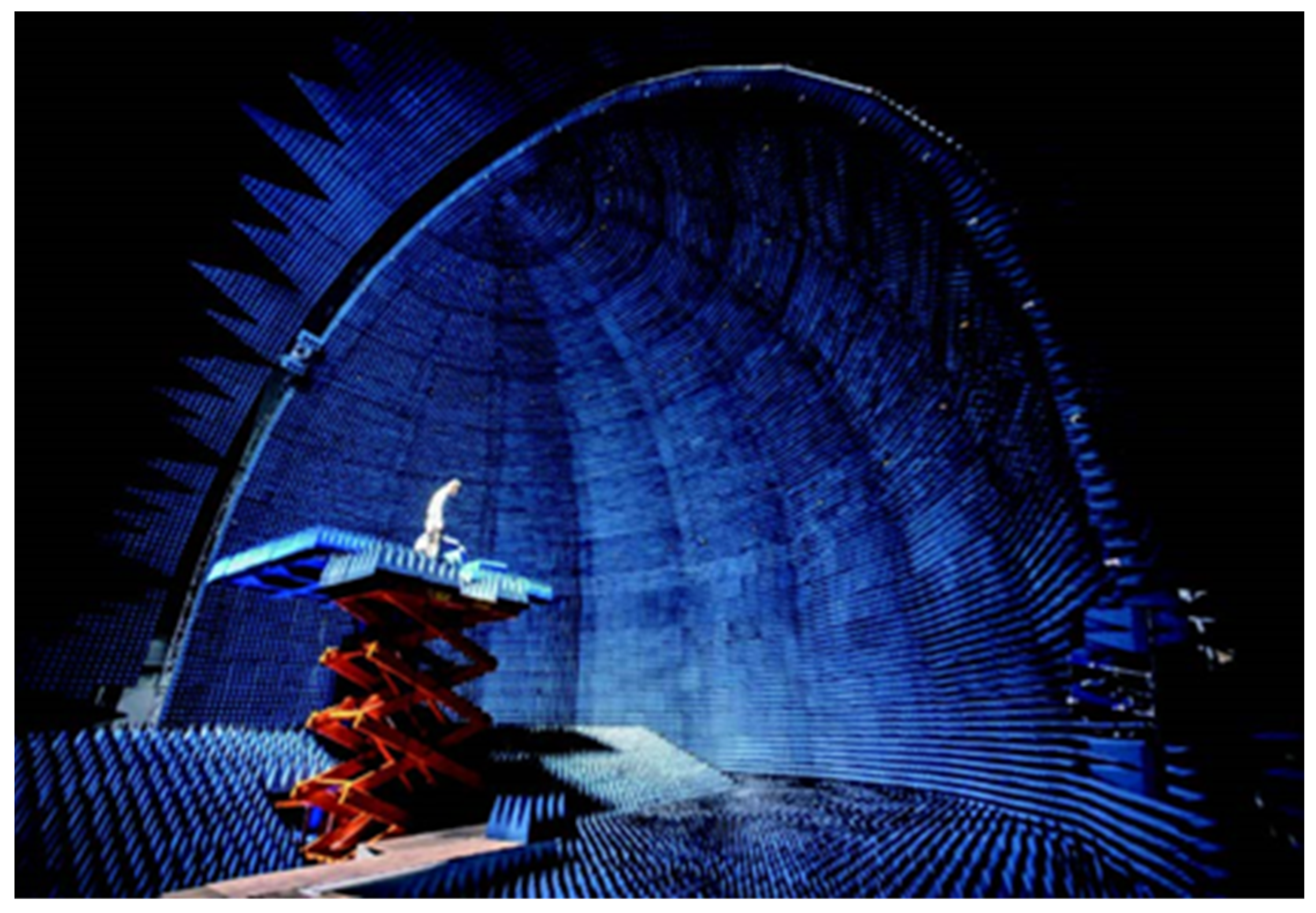
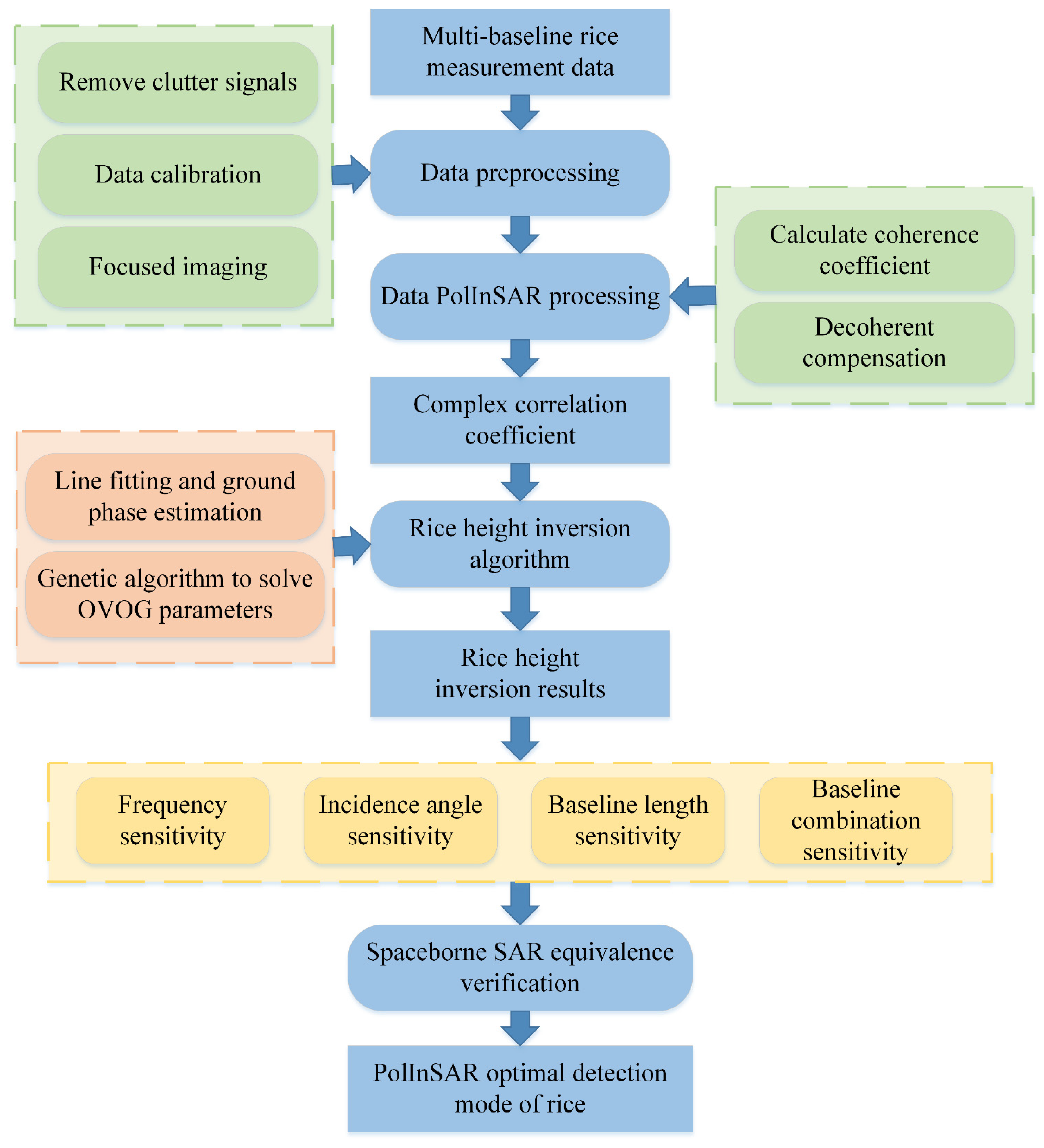
To address the issue of insufficient multi-baseline PolInSAR data, this paper conducted rice height inversion using the OVoG model, utilizing PolInSAR data obtained from the Laboratory of Microwave Properties (LAMP). LAMP serves as a scientific microwave anechoic chamber for land-target microwave characteristic measurement and simulation. Exploiting the versatile and controllable features of the microwave anechoic chamber, we obtained measurement data with continuous frequency bands, multiple baselines, and multiple incidence angles. A comprehensive investigation was conducted to analyze the impact patterns of factors such as frequency bands, baseline length, number of baselines, baseline combinations, and incidence angles on the inversion of rice plant height, aiming to provide insights into the optimal detection mode for rice height inversion. Furthermore, considering the imaging characteristics of the LAMP anechoic chamber, we explored the equivalence between microwave anechoic chamber measurement data and satellite data. This exploration led to the identification of the optimal detection mode for PolInSAR satellite rice height inversion based on microwave anechoic chamber results. This study furnishes reliable data support for the design and preliminary validation of future Synthetic Aperture Radar (SAR) satellite polarization interference measurement capabilities.
3. Results and Discussion
Based on the LAMP microwave anechoic chamber measurement data, the described research method was used to achieve rice height inversion, and an analysis was conducted to investigate the impact of various factors, such as the incidence angle, frequency band, baseline length, and baseline combination, on the accuracy. A root mean square deviation and a mean average deviation (MAE) were used as evaluation metrics for the algorithm.
3.1. Effect of Incidence Angle
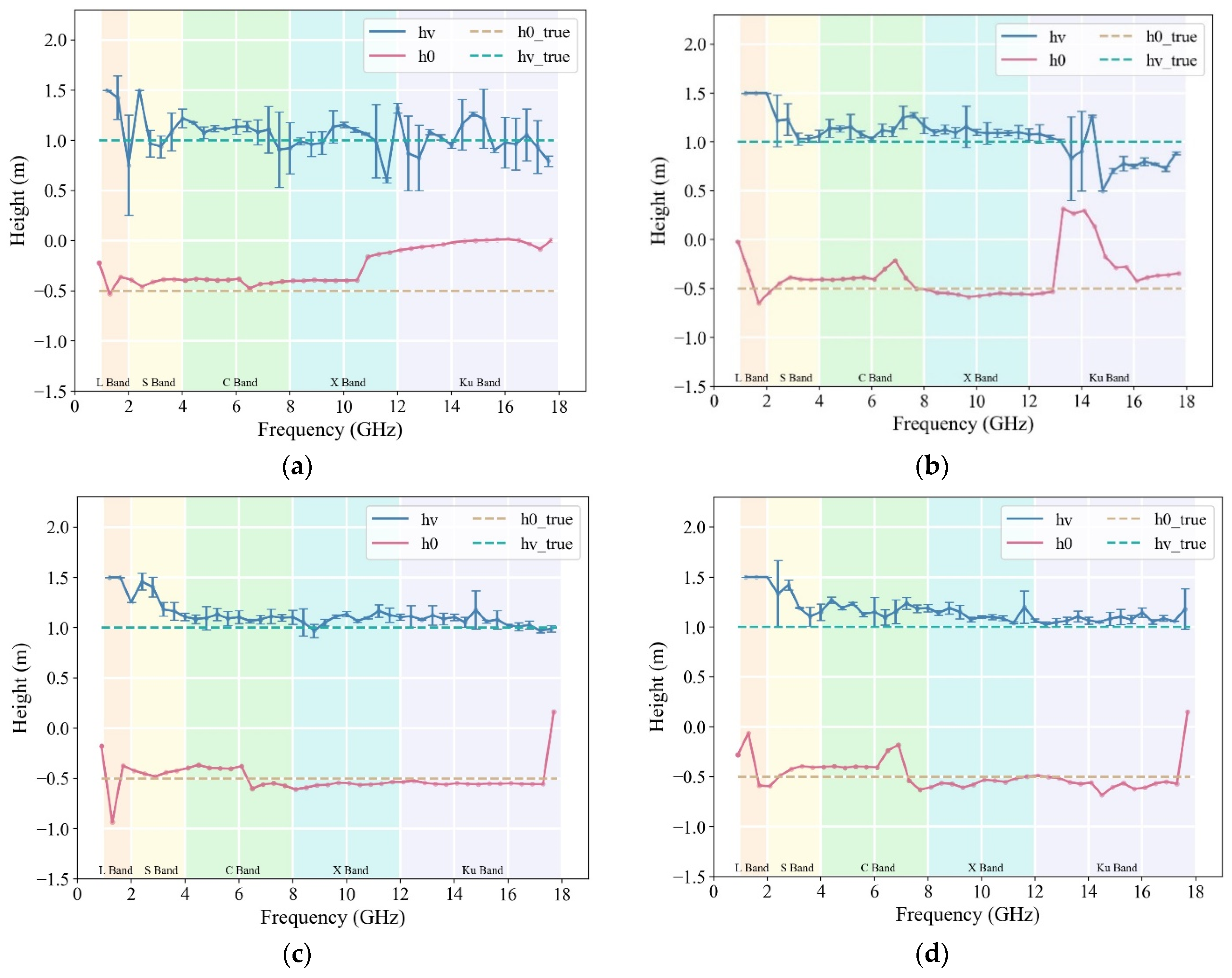
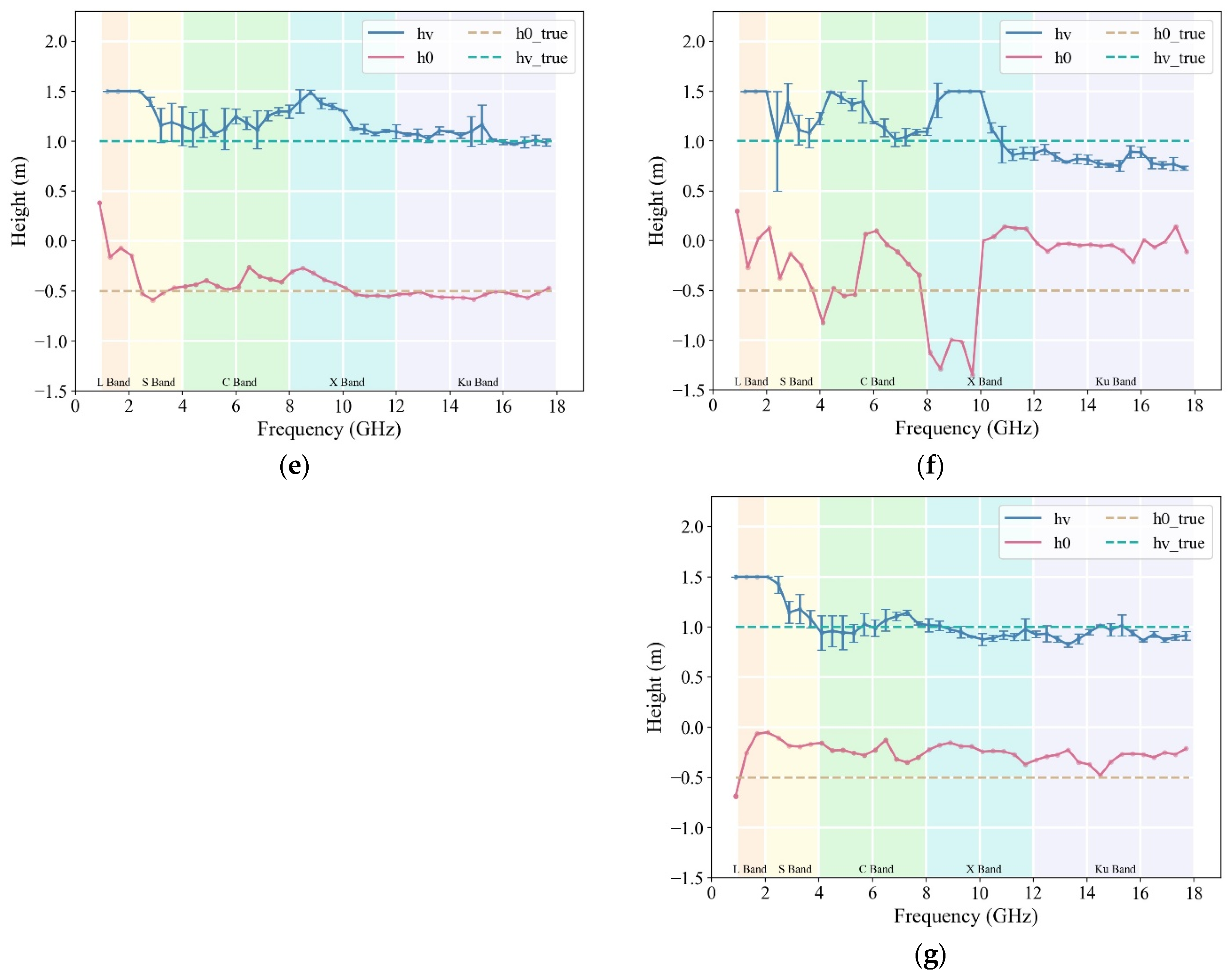
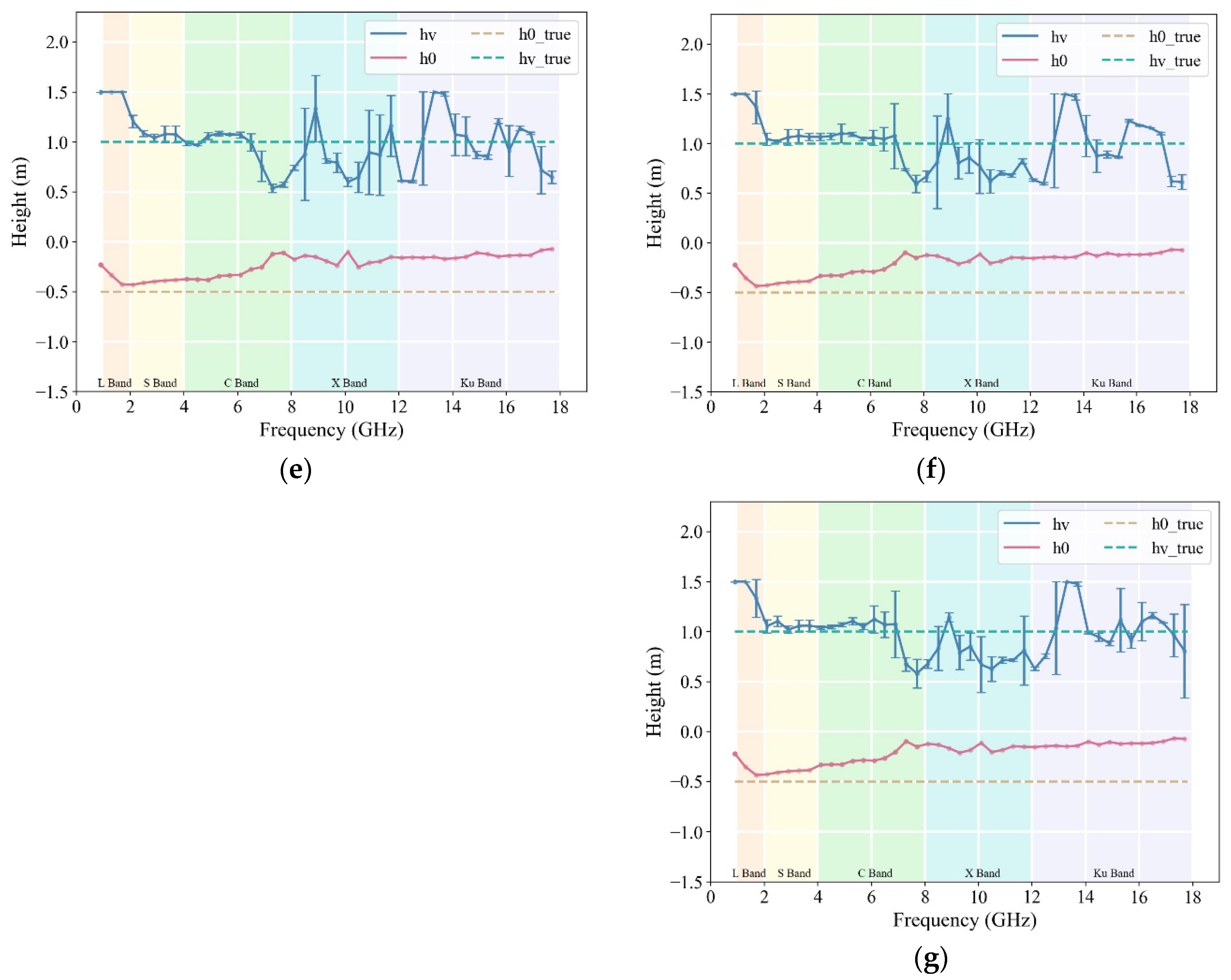
Example measurements with a 0.25° baseline and data in the 0.8–18 GHz range were used to examine the influence of seven different incidence angles ranging from 15° to 75° on rice plant height retrieval accuracy to effectively analyze the impacts of different incidence angles on the accuracy of rice plant height retrieval. The estimated values for rice height and ground-phase height under the conditions of a 0.25° baseline, 0.8–18 GHz frequency range, and incidence angles ranging from 15° to 75° with a 10° interval are shown in
Figure 5a–g.
Various polarized electromagnetic waves can effectively interact with the rice canopy and the underlying surface with a 35° incidence angle, allowing the reflected signals to better capture this information (
Figure 5). The RMSE and MAE for the rice plant height retrieval were 0.1932 m and 0.1358 m, respectively. Furthermore, optimal retrieval performance was observed in the incidence angle range of 35–55° and frequency range of 10–17 GHz (X and Ku bands).
The accuracy of the surface phase height estimation in the high-frequency band (13 GHz) was poor when the incidence angle was <35°. This indicates that the penetrating ability of high-frequency electromagnetic waves is limited at smaller incident angles, and they cannot adequately reflect information from the underlying surface. The X-band band struggled to effectively estimate the surface phase height at a 15° incidence angle. In addition, there was a significant estimation error in the height of the Ku-band surface phase at a 25° incidence angle. However, the retrieval results of the lower-frequency bands still maintained a good level of accuracy at lower incidence angles. For example, the inversion MAE for the C-band was 0.1595 m at a 15° incidence angle, whereas the X-band inversion MAE was 0.1176 m at a 25° incidence angle.
The propagation path of the electromagnetic waves through the rice layer was longer at incidence angles of 55°, resulting in significant signal attenuation and a diminished ability to effectively reflect information from the underlying surface. The overall accuracy of the surface phase estimation was notably poor at a 65° incidence angle, indicating that the signal attenuation is substantial when the propagation path is extended.
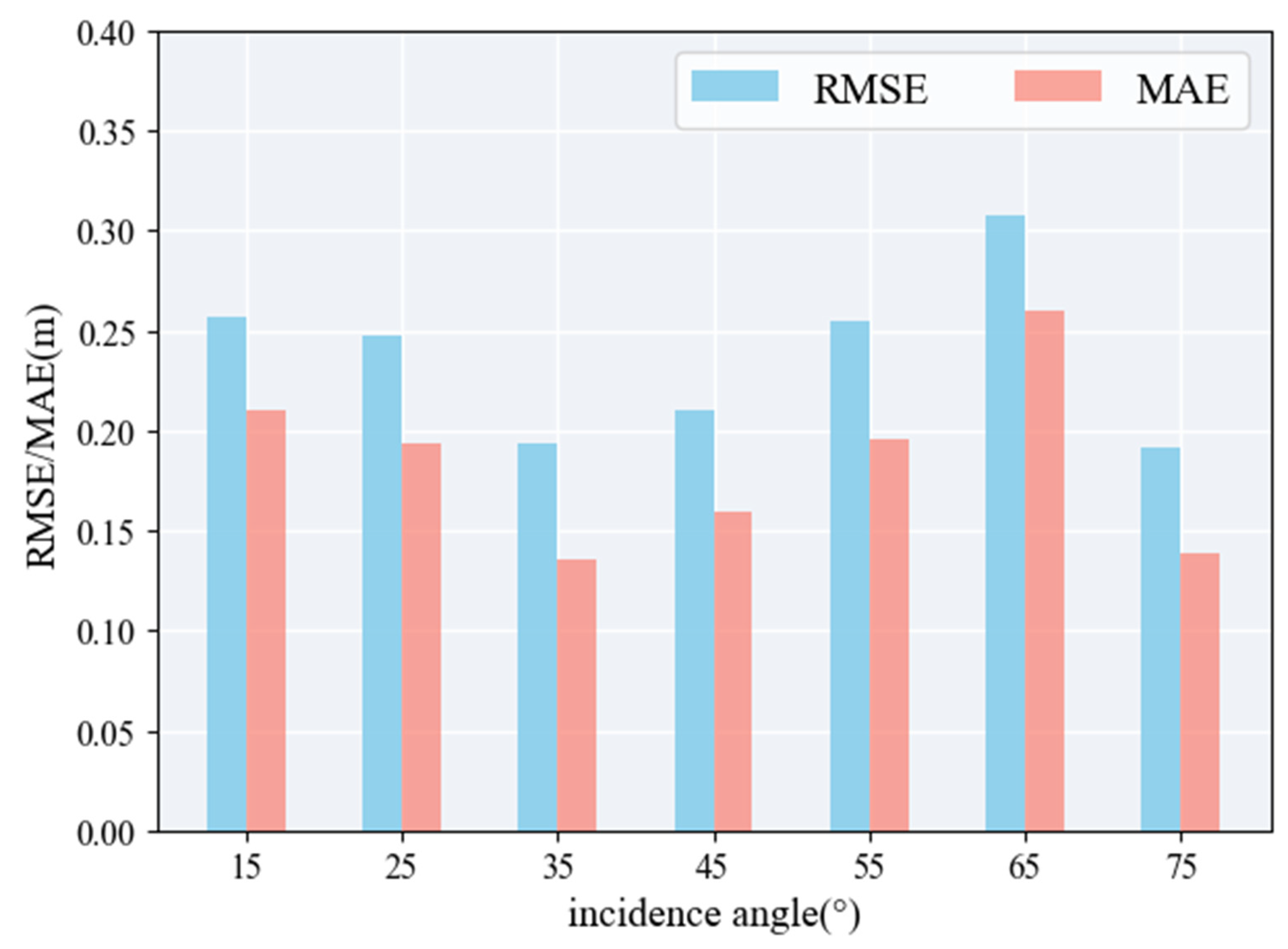
The RMSE and MAE calculated for rice height estimates across different incidence angles (15–75°) within the 0.8–18 GHz frequency range are shown in
Figure 6. The accuracy of rice plant height inversion initially increased with a greater incidence angle and then decreased with a larger incidence angle after 35°. The MAE for plant height estimation at a 35° incidence angle was the smallest, at 0.1359 m. The precision of vegetation height estimation was the lowest at a 65° incidence angle, with an RMSE of 0.3073 m and an MAE of 0.2598 m. This resulted in significant fluctuations in the estimated ground-phase. The advantage of the combined method lies in its ability to provide precise estimates of the ground-phase owing to the ground volume interaction of rice. However, the accuracy of the rice height estimation is compromised when there is a significant error between the estimated ground-phase values and the true values because the ground-phase serves as one of the input parameters for the optimization algorithm. Notably, the rice height estimation accuracy was relatively high at a 75° incidence angle, with an RMSE of approximately 0.1920 m and an MAE of approximately 0.1385 m. The highest accuracy for rice plant height inversion was obtained when the incidence angle of the radar data was 35–55° according to the analysis of rice plant height inversion results under different incidence angles.
3.2. Effects of Baseline Length
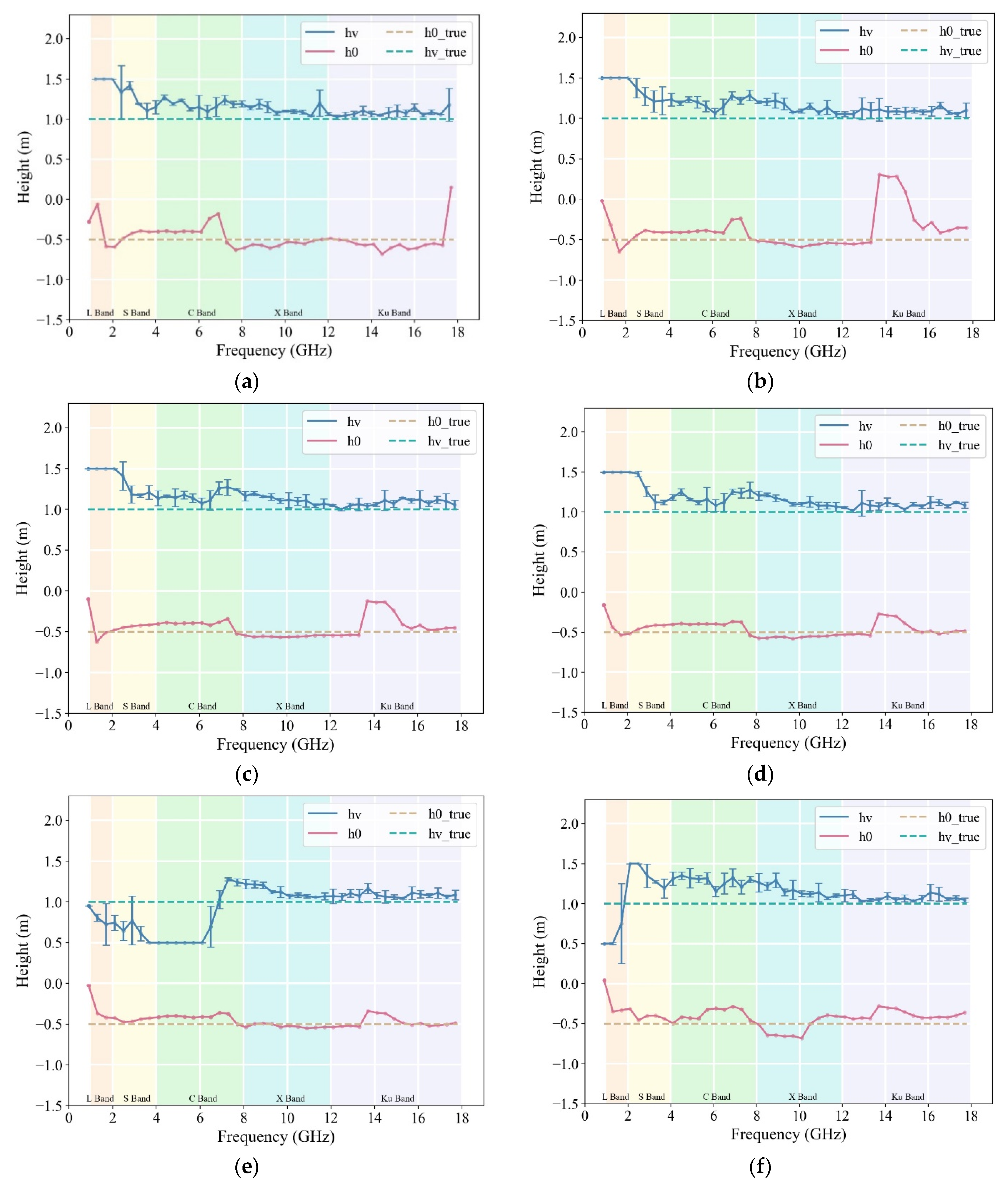
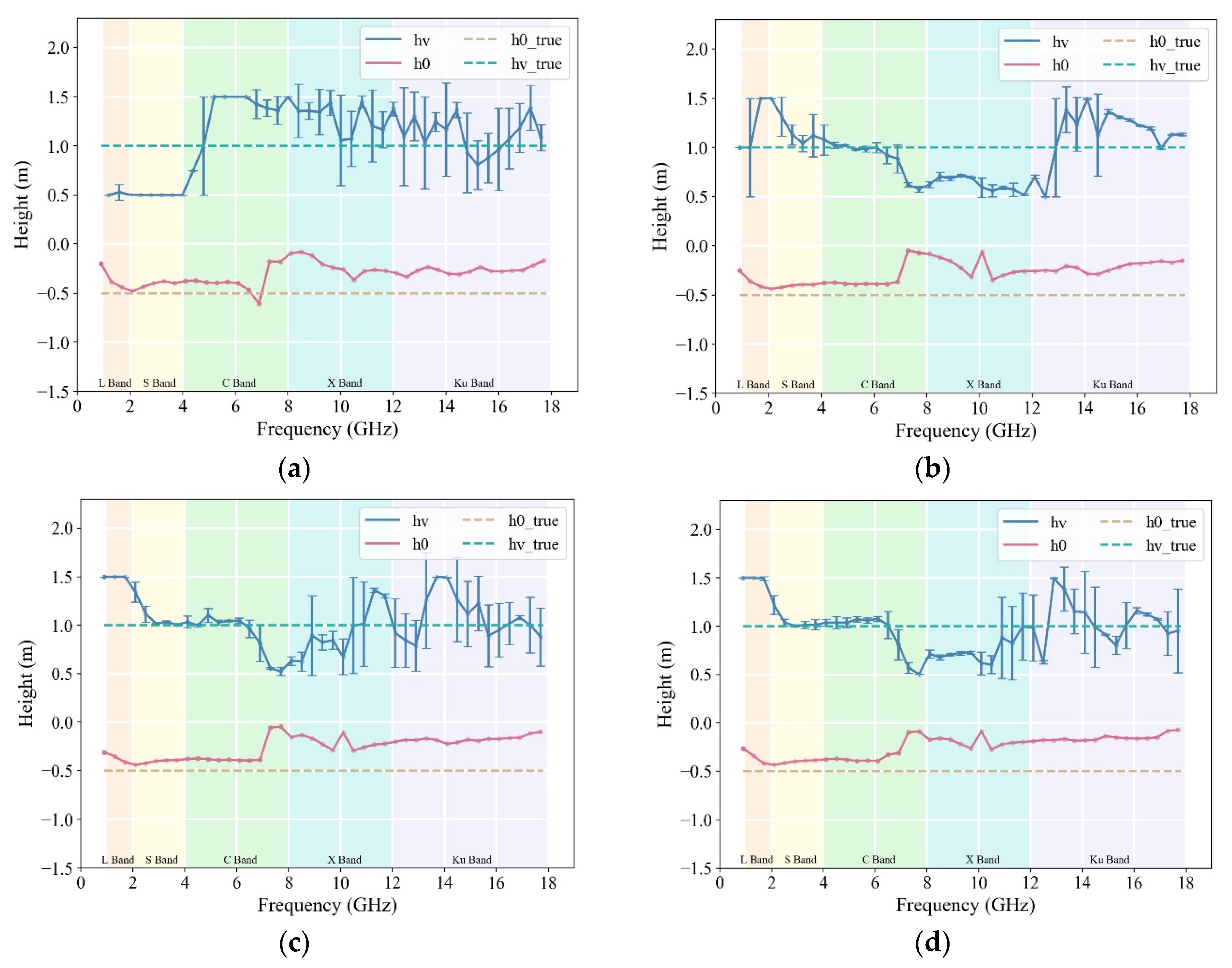
Measurement data at a 45° incidence angle within the 0.8–18 GHz range were analyzed to effectively analyze the influence of different baseline lengths on the accuracy of rice plant height retrieval. The impacts of eight different baseline lengths, ranging from 0.25° to 2° were assessed at a 45° incidence angle. The estimated values for rice plant height and ground-phase height under the conditions described are shown in
Figure 7a–g.
The best plant height inversion results were obtained with the 0.25° baseline condition, which showed good stability for all bands. The error between the estimated value of the surface phase and the true surface phase gradually increased as the baseline length increased, and the accuracy of the inversion results started to decrease in short-wave bands such as X and Ku, whereas more accurate rice plant heights could still be obtained in the C and S bands. The coherence of the PolInSAR data decreased when B > 1.0°. The stability of the inversion results for the C- and S-bands deteriorated, and accurate plant height inversion results could not be obtained in the whole frequency band from 0.8 to 18 GHz. The slope difference of the boundary line defining the coherent region is not a monotonic function of the baseline but shows fluctuations similar to a sine function and reaches zero for some baselines [
32]. It is necessary to use relatively long baselines to increase the sensitivity in the vertical structure of the vegetation when using the PolInSAR data for rice height inversion. However, the process of the baseline increase is somewhat limited as the spectral shifts exceed the bandwidth at a certain length, resulting in decorrelation and a decrease in coherence to the extent of becoming zero.
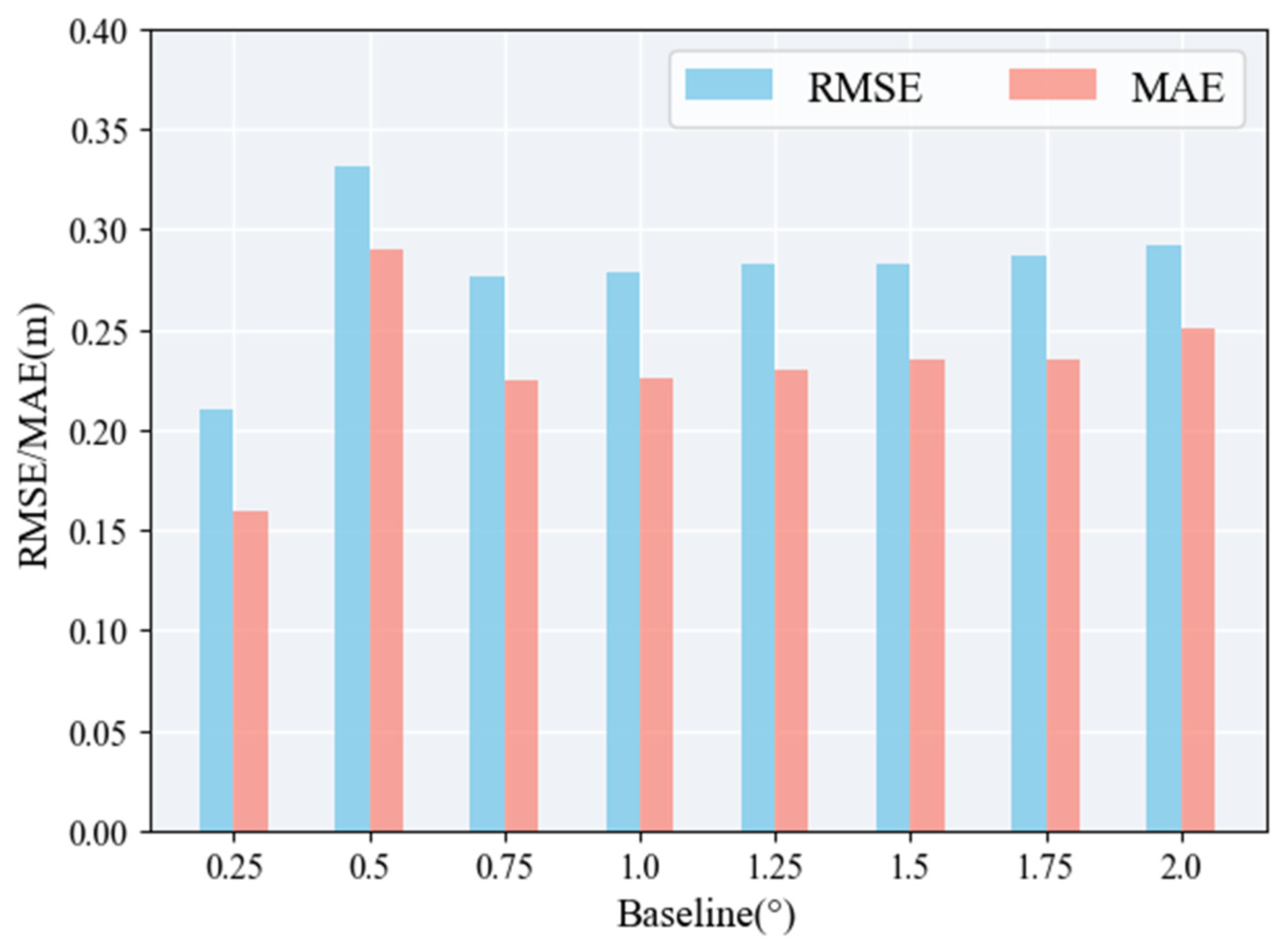
The RMSE and MAE of the rice height estimates calculated in the frequency range of 0.8–18 GHz for the baseline length of 0.25–2.0° are shown in
Figure 8. The values of the RMSE and MAE at B = 0.25° are both minimized to 0.1932 m and 0.1359 m, respectively, at an incidence angle of 45°, and the curves representing the ground-phase and vegetation height exhibited relatively stable variations. The ground-phase curve experienced notable fluctuations at B = 0.5°, and the plant height followed a similar trend, resulting in decreased accuracy with RMSE and MAE values of 0.2620 m and 0.2071 m, respectively. The RMSE and MAE approached approximately 0.3 m and 0.25 m, respectively, and exhibited a generally positive correlation with baseline length when B > 0.5°. Overall, the 0.25° baseline was the most suitable for rice height estimation. However, the selection of the optimal baseline length must consider the shape and structure of the target being measured. Research [
21,
33] on baseline lengths for forest height estimation suggests that shorter baselines can provide sufficient coherence for PolInSAR in terms of forest height retrieval owing to the higher average height of forests when compared with crops.
3.3. Effect of Baseline Combinations
3.3.1. Combination of Baselines with the Same Length
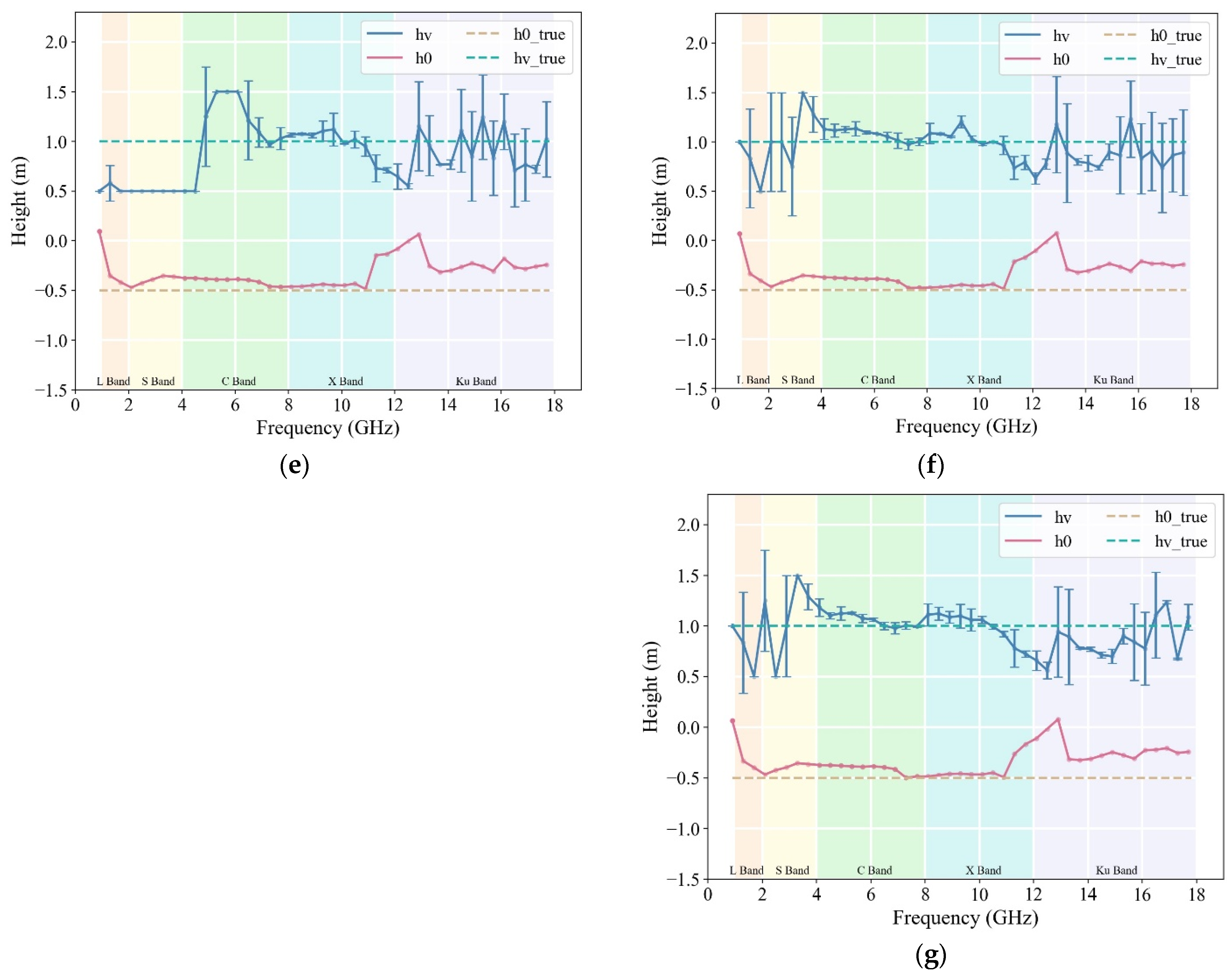
The effects of combining baselines of the same length on the inversion accuracy of rice height were analyzed at lengths of 0.25° and 0.5°, taking the 45° incidence angle and 0.8–18 GHz measurement data as an example. The estimated values of the rice height and ground-phase height under these conditions and incidence angles ranging from 15° to 75° are shown in
Figure 9a–h and
Figure 10a–g.
Under the 0.25° baseline, combinations of one to four baselines yielded accurate rice height estimates in both the C- and Ku bands. The stability of the algorithm for rice height retrieval increased with an increase in the number of baselines. However, the rice height resulted in an L-band transition from overestimation to underestimation when five baselines were used, and there was a decrease in accuracy in the S- and C-bands. Obtaining accurate rice height estimates with one baseline becomes challenging under a 0.5° baseline. Combining two to three baselines results in a higher accuracy in rice height estimations within the C-band. The proportion of accurate rice height estimates shifted to the X-band with four to five baselines. Under six to seven baselines, the increased number of baselines expands the observation space, allowing for the C- and X-bands to achieve higher estimation accuracy.
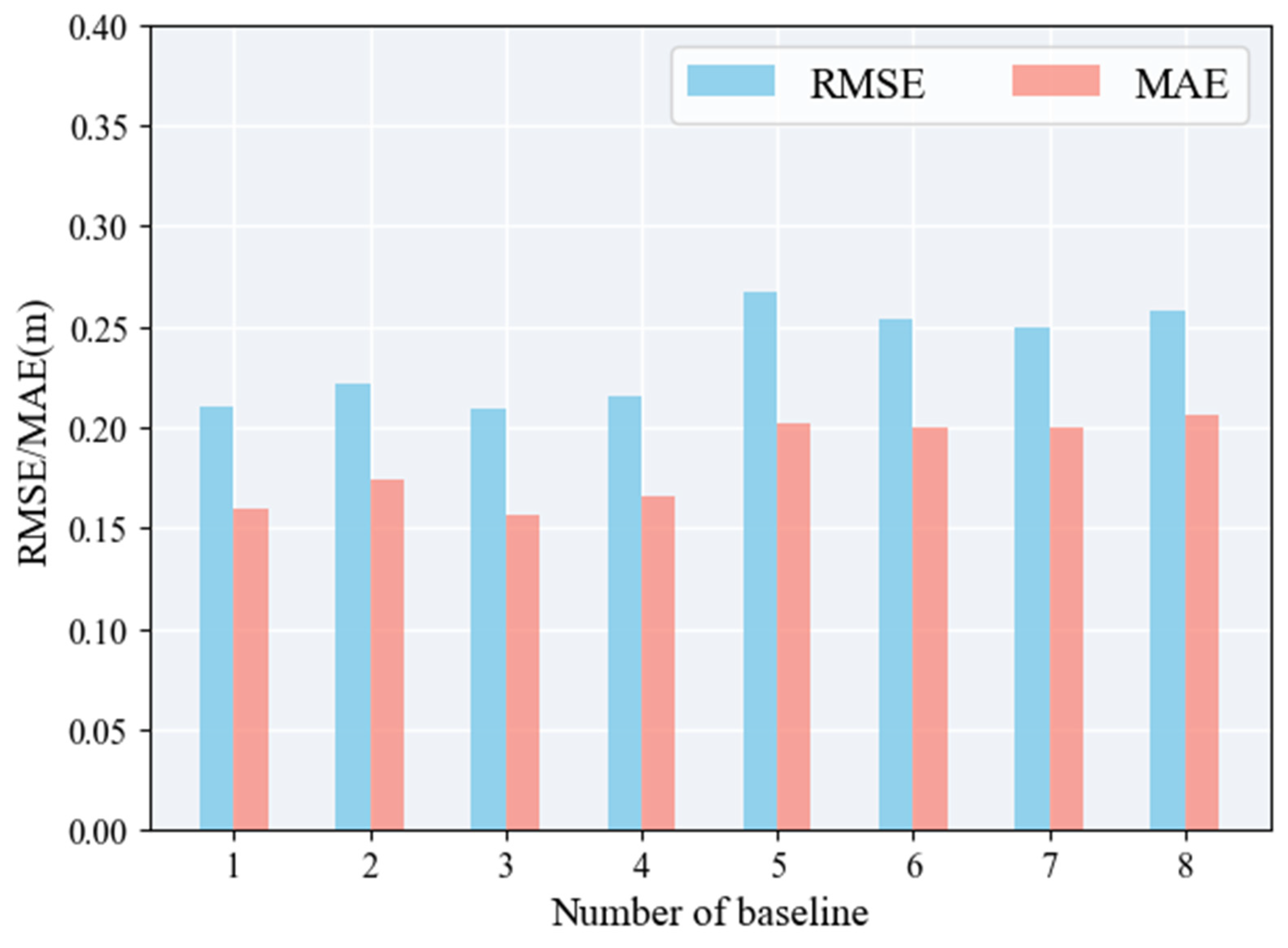
The RMSE and MAE calculated for rice height estimations in the 0.8–18 GHz frequency range using the same baseline combinations under 0.25° and 0.5° baseline lengths are shown in
Figure 11 and
Figure 12. When utilizing 0.25° multi-baseline combinations for rice height retrieval, the accuracy of plant height does not increase with the number of baselines; instead, it follows a trend of initially increasing and then decreasing. The highest accuracy was achieved with a combination of the three baselines, yielding an RMSE of 0.2094 m and an MAE of 0.1560 m. When five baselines were used, the RMSE and MAE values reached their maxima at 0.2669 m and 0.2019 m, respectively. Furthermore, the accuracy of the algorithm is superior with one to four baselines when compared with five to eight baselines.
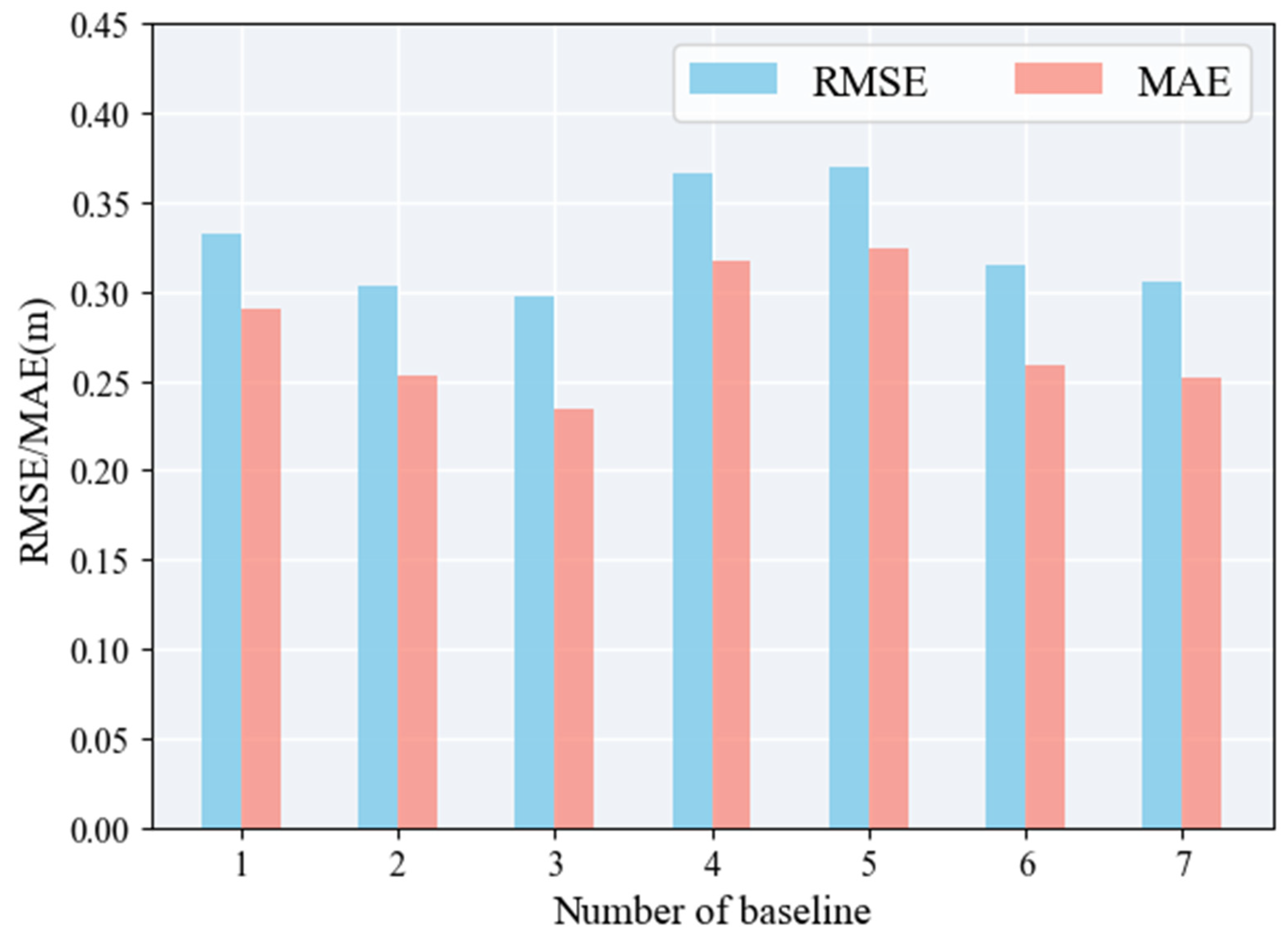
The rice height estimation results for 0.5° multi-baseline combinations exhibited the same trend as those for 0.25° (
Figure 12). The highest accuracy was achieved with three baselines, with an RMSE of 0.2967 m and an MAE of 0.2340 m, whereas the accuracy decreased significantly when four baselines were used, and the worst accuracy were achieved with five baselines. Within a certain range of baseline numbers, having more baselines of the same length can expand the observation space, reduce the variance and bias of the rice height estimation results, and enhance the stability of the retrieval outcomes. However, an excessive number of baselines limits the increased observation space, and a larger dataset may lead the algorithm to the local optima. Pichierri et al. [
19] conducted Monte Carlo simulations to study the relationship between the number of baselines and the RMSE of corn height retrieval. They found that the RMSE negatively correlated with the number of baselines. However, further increases did not significantly reduce the estimation error when the number of baselines reached five. The conclusions drawn in this study regarding rice height retrieval and the number of baselines agree with Pichierri et al. [
19].
3.3.2. Combination of Baselines with Different Lengths
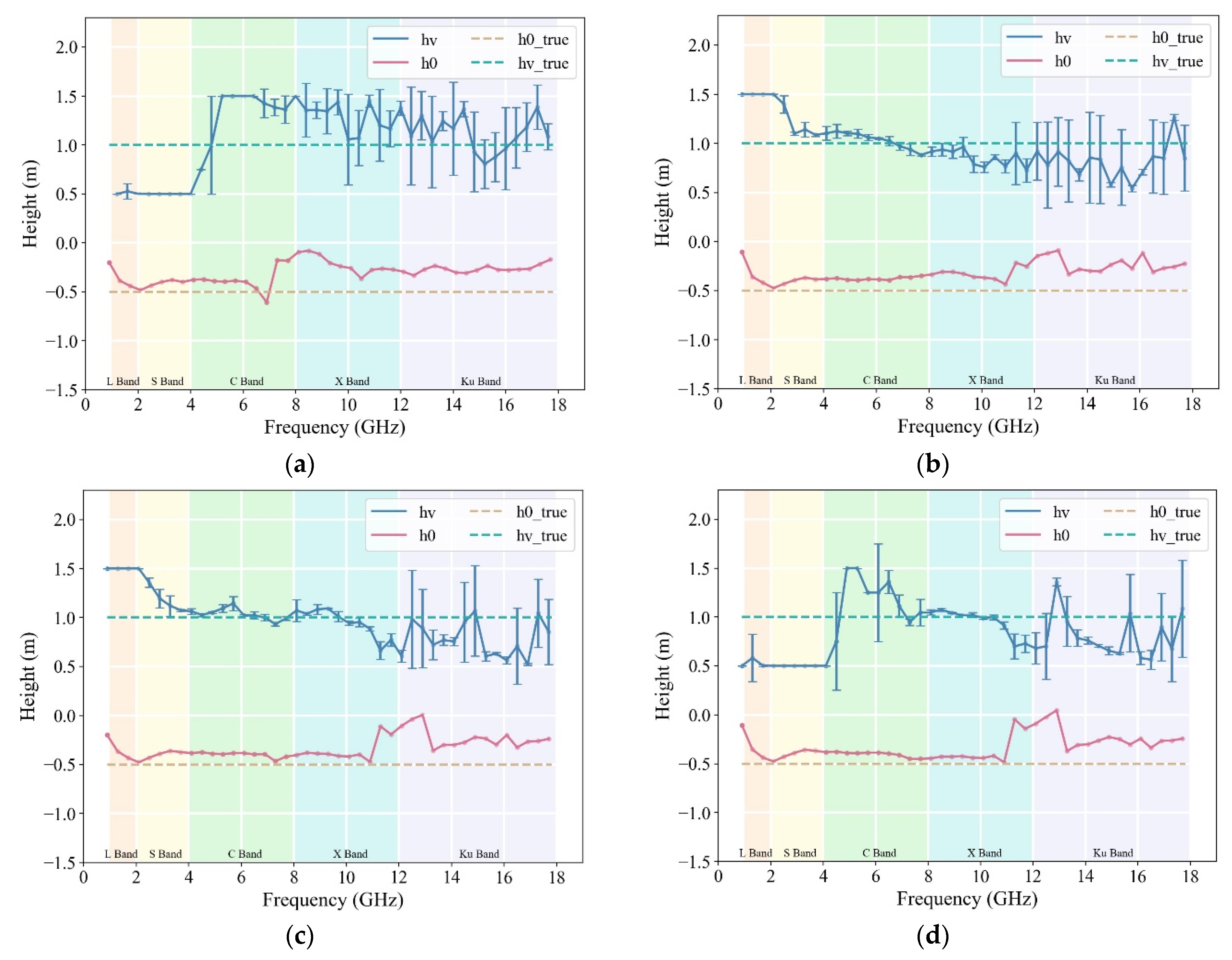
The effect of the combination of baselines of different lengths on the inversion accuracy of rice height was analyzed with the 45° incidence angle and 0.8–18 GHz measurement data as examples. The 0.5° baseline was the base, and then successively increased by 0.75°, 1°, 1.25°, 1.5°, 1.75°, and 2° to analyze the effects of baseline combinations of different lengths on the accuracy of vegetation height inversion.
The RMSE and MAE calculated for different baseline combinations of rice height inversion based on the 0.5° baseline in the frequency range of 0.8–18 GHz are shown in
Figure 13a–g. It is difficult to obtain accurate estimates of rice height using a 0.5° single baseline, and the accuracy improves in the S- and C-bands when three to four baselines are used for inversion. The accuracy of the rice height inversion was further improved in the X- and Ku-bands as the number of baselines increased from five to seven.
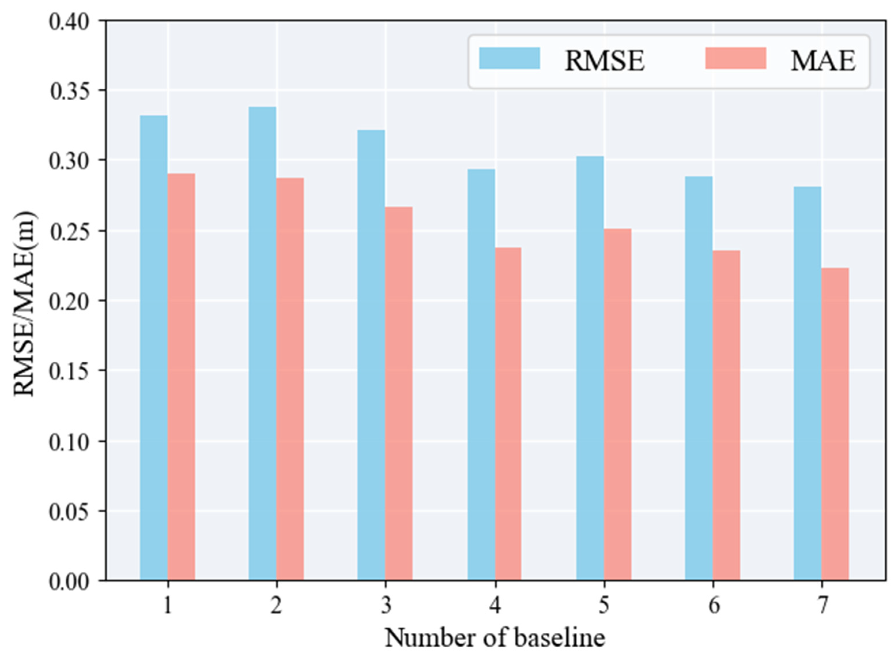
The RMSE and MAE of the rice height estimates for combinations of different baseline lengths based on a 0.5° baseline over a frequency range of 0.8–18 GHz are shown in
Figure 14. The accuracy of rice height estimates increased as the number of baselines increased for different combinations. The accuracy of rice height estimates was the poorest with two baselines, since the RMSE and MAE values were 0.3381 m and 0.2873 m, respectively. The accuracy of the rice height estimation was highest with seven baselines, with RMSE and MAE values of 0.2804 m and 0.2231 m, respectively. The RMSE and MAE increased by approximately 0.05 m and 0.03 m when the number of baselines increased from one to four. However, the RMSE and MAE only increased by approximately 0.01 m as the number of baselines increased from four to seven. Longer baselines with a B > 1.5° exhibit a less significant improvement in accuracy owing to reduced coherence. Different baseline combinations can enhance the accuracy of rice height retrieval by expanding the observation space. However, it is essential to carefully select the baselines added to the combinations to maintain accuracy.
3.4. Optimal Baseline Combinations
From the preceding analysis, it is evident that the optimal range for rice plant height retrieval occurs at incidence angles between 35° and 55° with a baseline of 0.25°. Three to four baselines resulted in the highest accuracy in rice plant height retrieval and were identified as the optimal baseline quantity. In pursuit of optimal system parameters for rice plant height inversion, a combination of the best baseline length, quantity, and incidence angle within the identified optimal ranges was selected to further optimize inversion performance.
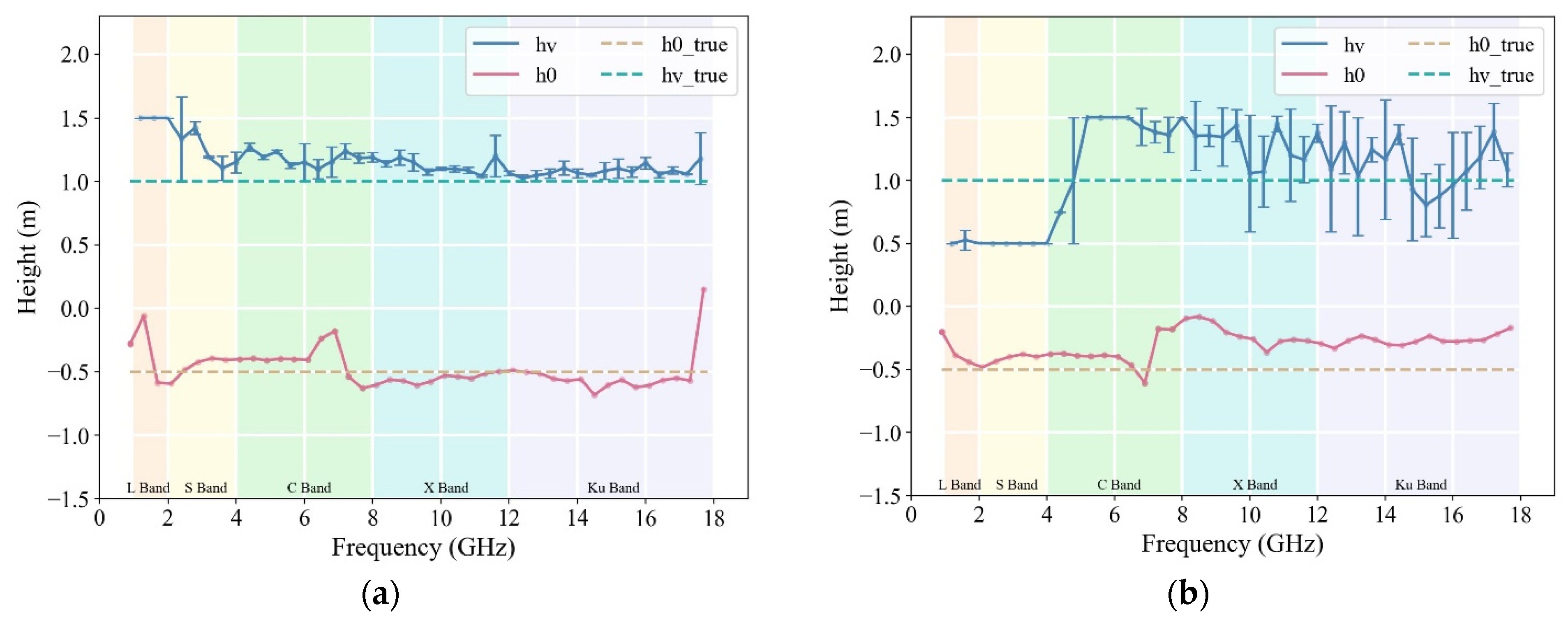
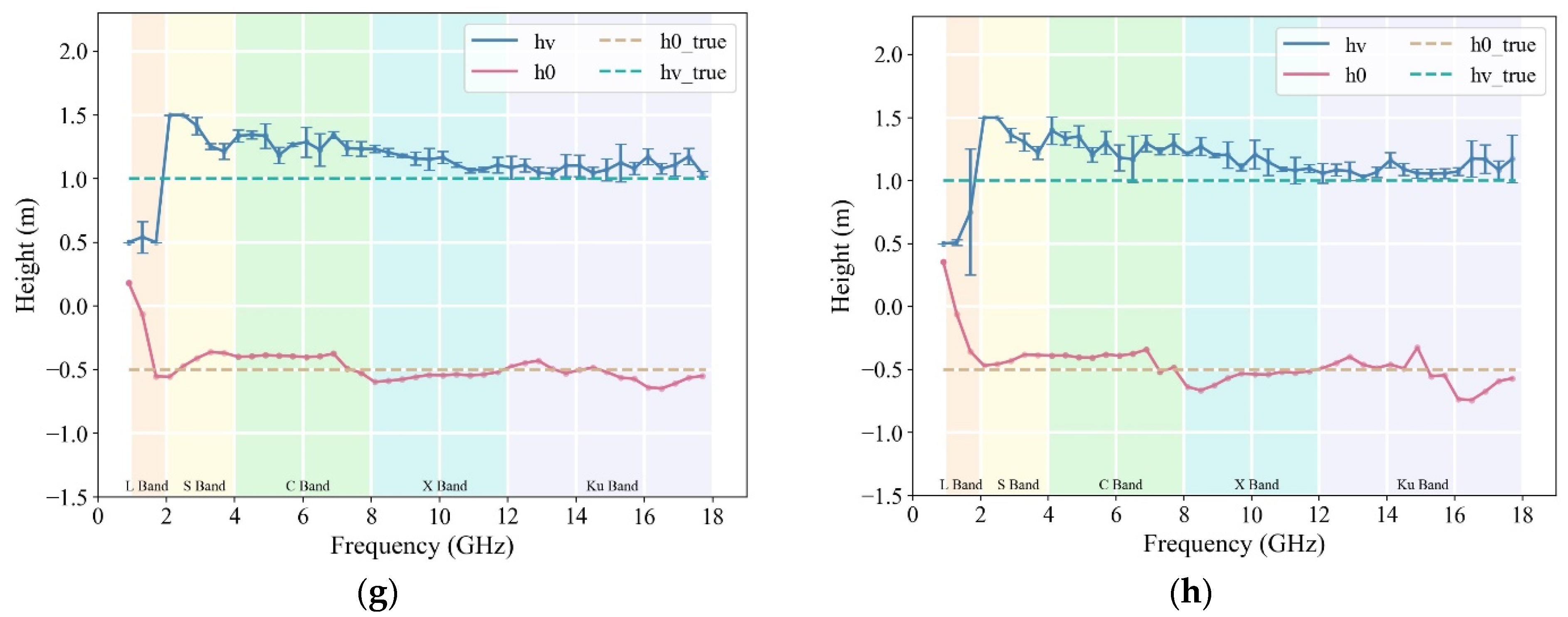
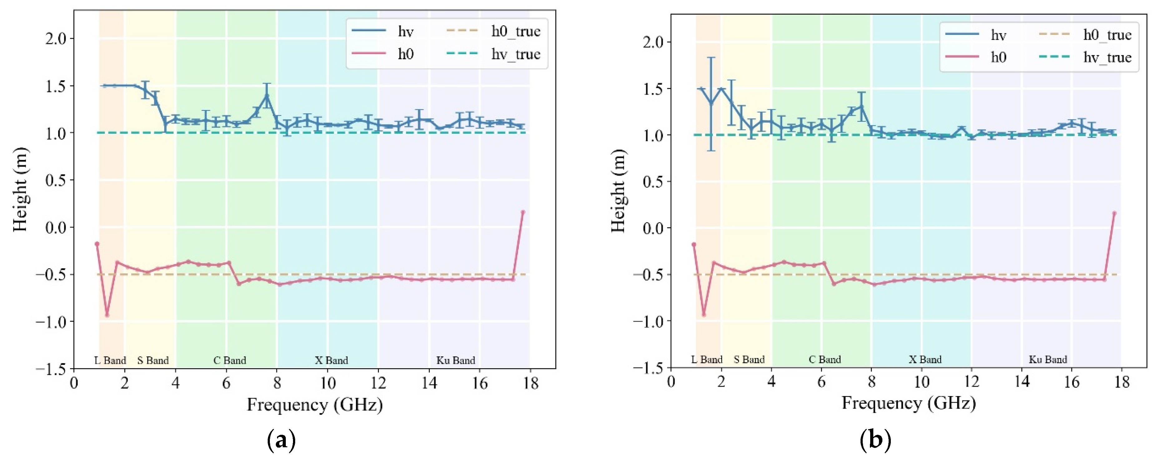
The first combination selected three baselines of 0.25° each at incidence angles of 35°, 45°, and 55° for the rice plant height inversion (
Figure 15a). The curves of the surface phase and vegetation height inversion exhibited smooth profiles with a noticeable peak at approximately 6 GHz. The corresponding RMSE and MAE values were 0.2148 m and 0.1636 m, respectively, indicating a high level of accuracy in the inversion results. The second combination (building on the first) introduced an additional baseline of 0.5° at an incidence angle of 55°. The inversion results depicted in
Figure 15b reveal an improved fit of the surface phase and vegetation height inversion curves to the ground truth. In particular, the error was less than 8 cm in the high-frequency portion > 7.5 GHz. The RMSE and MAE values were 0.1758 m and 0.1093 m, respectively, representing the highest accuracy among all the baseline combinations. This underscores the importance of selecting the preferred baseline combinations to improve the sensitivity of vegetation height retrieval algorithms to PolInSAR data.
In terms of selecting the incident wave frequency, the performance of the algorithm was relatively poor in the L-band and even in the lower frequency bands. Low-frequency waves exhibit strong penetration capabilities through vegetation, making it challenging to detect rich vertical information for low-lying crops. Short baseline data may result in overestimation of the S-band; however, the S-band can also achieve improved results with the selection of optimal baseline combinations. The C-, X-, and Ku-bands all exhibit strong retrieval capabilities and potential, making them the preferred frequency bands for the future retrieval of plant height for low-lying crops such as rice. These parameters can better facilitate the retrieval of vertical structural parameters, including plant height, for low-lying crops such as rice when combined with the optimal spatial baseline combinations proposed in this study.
3.5. Equivalence Analysis of the LAMP Microwave Anechoic Chamber with On-Board SAR Imaging Geometry
The LAMP microwave anechoic chamber strives to simulate the imaging geometry of spaceborne SAR satellites to the greatest extent possible. However, certain differences still exist, primarily in imaging modes, signal acquisition, imaging principles, and other aspects. Therefore, equivalence must be considered to extend the research findings from the LAMP microwave anechoic chamber to practical applications in spaceborne SAR systems. Given the complexity of equivalence problems, this study focuses primarily on the simplest form of imaging geometry equivalence.
An equivalency analysis was conducted using imaging geometry from a domestically developed SAR satellite (GF-3 satellite) with polarimetric and interferometric measurement capabilities as an example. Building on this analysis, conclusions drawn from the LAMP microwave anechoic chamber were extended and applied to spaceborne SAR satellites. Specifically, an optimal detection mode for spaceborne SAR was proposed by focusing on rice height retrieval. This study provides a scientific basis for the design of future spaceborne SAR systems and their subsequent applications.
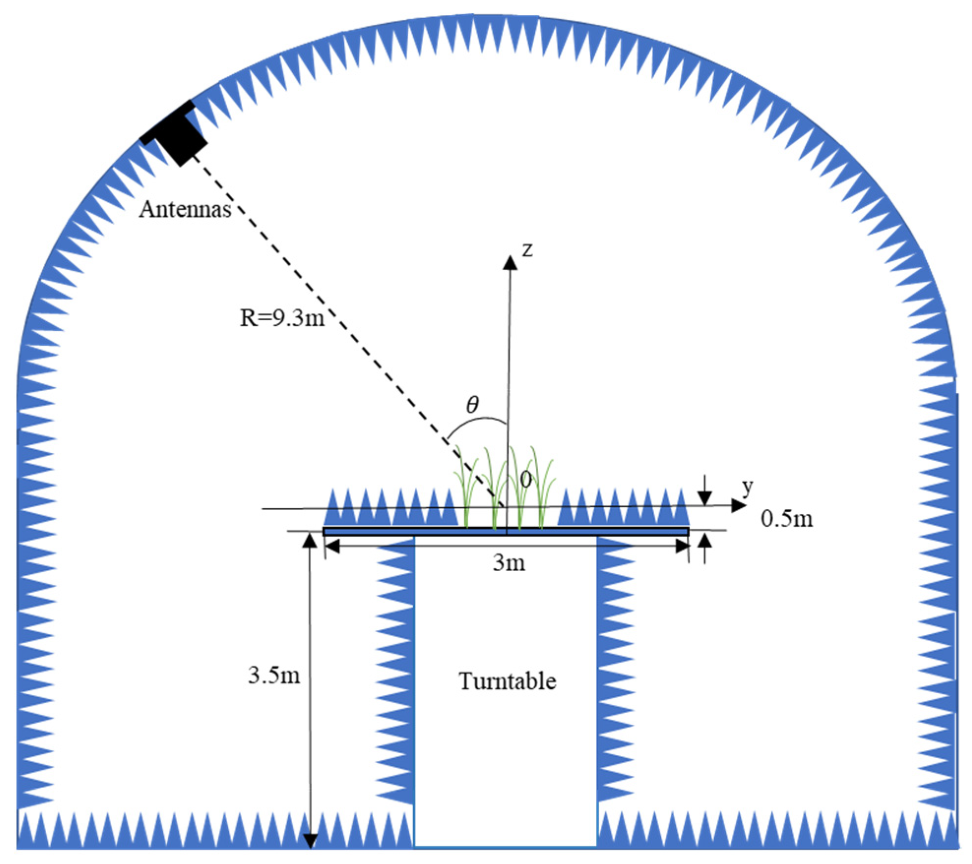
The slant distance of the LAMP microwave anechoic chamber is the distance from the dome antenna to the focus point of the platform, which is 9.3 m. However, in the actual experiment, the imaging position of the platform is 15 cm above the focus point of the platform, and according to the calculation, the actual slant distance should be 9.19 m. The orbital altitude of the GF-3 SAR satellite was 755 km, and the slant range of the GF-3 satellite was calculated based on the orbital altitude and incidence angle. By establishing the imaging geometry equivalence relationship between the LAMP microwave anechoic chamber and the GF-3 SAR satellite, the imaging geometry equivalence relationship between them can be constructed. The geometric equivalence relationship between the LAMP microwave anechoic chamber and the vertical baseline of the SAR satellite is as follows:
where
and
denote the slant distances of the GF-3 satellite and the LAMP microwave anechoic chamber, respectively, and the
and
denote the vertical spatial baseline lengths corresponding to the interferometric measurements of the GF-3 satellite and the LAMP microwave anechoic chamber, respectively.
The spatial baseline of the LAMP microwave anechoic chamber was measured in terms of angles. In the actual calculations, the spatial baseline measured in degrees was first converted into a spatial baseline measured in units of distance. Geometric equivalency formulas were then used to establish the geometric spatial relationship between the LAMP microwave anechoic chamber and the GF-3 satellite. When the incidence angle was 35°, the optimal spatial baseline lengths for the LAMP microwave anechoic chamber were calculated to be 0.25° and 0.50°, corresponding to the vertical spatial baseline lengths of the SAR GF-3 satellite system, as shown in
Table 3.
Vertical wavenumber is an important parameter for rice height inversion, and its magnitude is closely related to the PolInSAR retrieval of vegetation height. When is excessively large, the coherence of PolInSAR decreases, leading to the risk of oversaturation in vegetation height retrieval, where heights above a certain threshold are underestimated. On the other hand, when is too small, the sensitivity to the vertical structure of vegetation is reduced, making the height retrieval process susceptible to errors resulting from parameter variations. Different types of vegetation have specific ranges of vertical wave numbers that correspond to optimal PolInSAR measurement modes. By using measurement modes within these ranges, higher-precision vegetation height retrieval results can be obtained for vegetation of the respective type and height.
In the LAMP microwave anechoic chamber, the baseline vertical wave number was represented using the incidence angles. In spaceborne SAR systems, this baseline can be expressed in terms of the vertical spatial baseline length, where
represents the wavelength of the incident wave,
is the interferometric vertical spatial baseline,
is the slant range from the antenna to the target, and
is the incidence angle of the main interferometric image.
Based on the optimal incidence angle of 35–55° and an optimal baseline length of 0.25°, the vertical wavenumber under the optimal baseline combination was calculated from the derived conclusions (
Table 4), and the minimum value of the vertical wavenumber was 1.04, with a maximum value of 4.05.
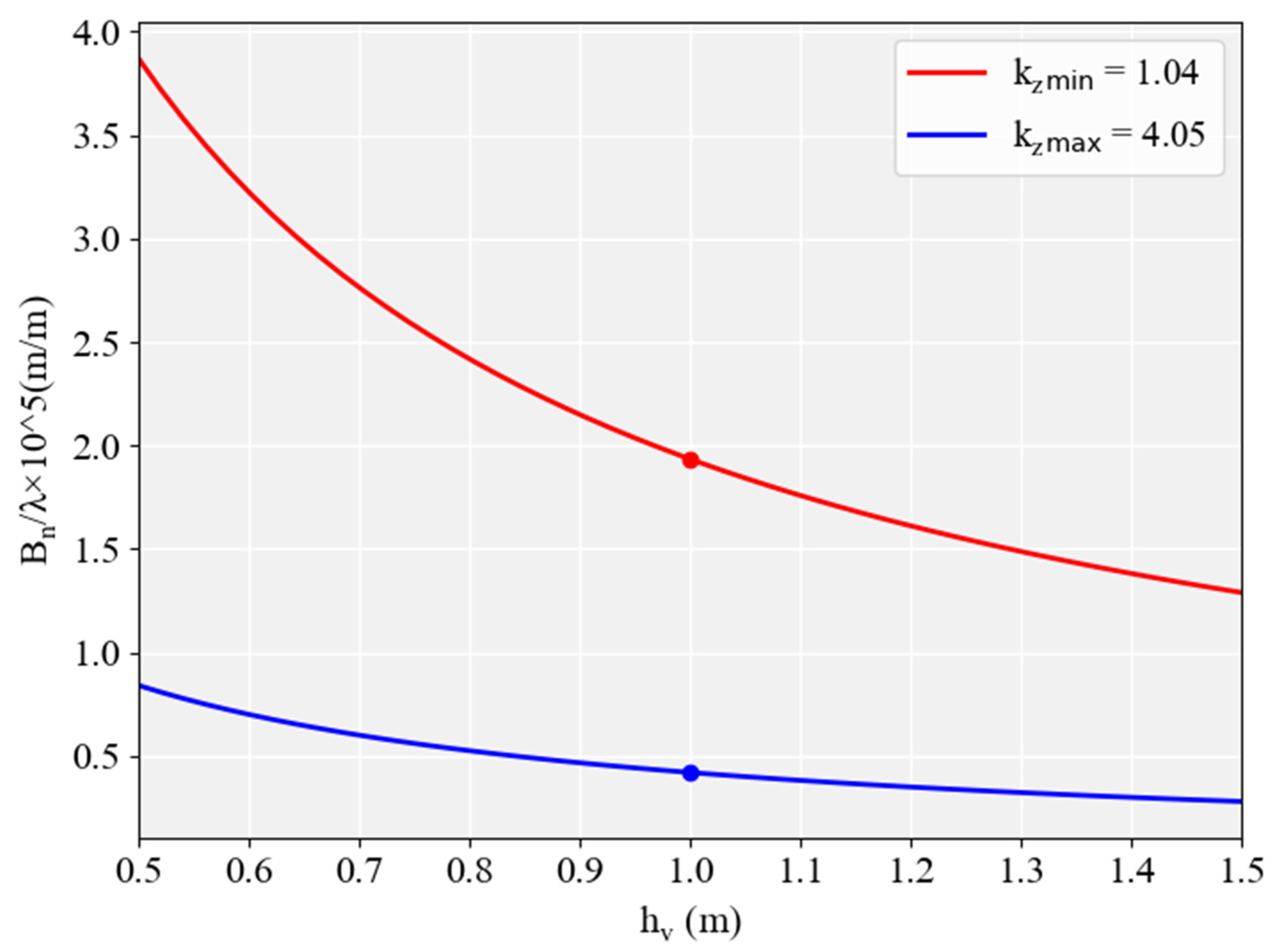
Cloude and Papathanassiou [
34] proposed to use the product of the vertical wave number and the vegetation height to
to describe the optimal range of vegetation height inversion [
12]. Based on the range of
obtained during the experimental process, an example is provided using a 35° incidence angle and a GF-3 satellite orbit height of 755 km to establish the functional relationship between
and
(
Figure 16). The two curves represent the upper and lower limits of the normal baseline wavelength ratio calculated based on the maximum
and minimum
of the vertical wavenumber, and the design of the spaceborne SAR will also be subject to the ratio
which must be contained within the region plotted in
Figure 16. The range of
is 0.44–1.93 for the previously studied rice field with a height of 1 m.
Fixing the slant distance parameter
at 921.68 km and a baseline length of 0.25° gives two curves of the optimal vertical spatial baseline length versus frequency based on the minimum and maximum values of the optimal vertical wavenumber range, respectively (
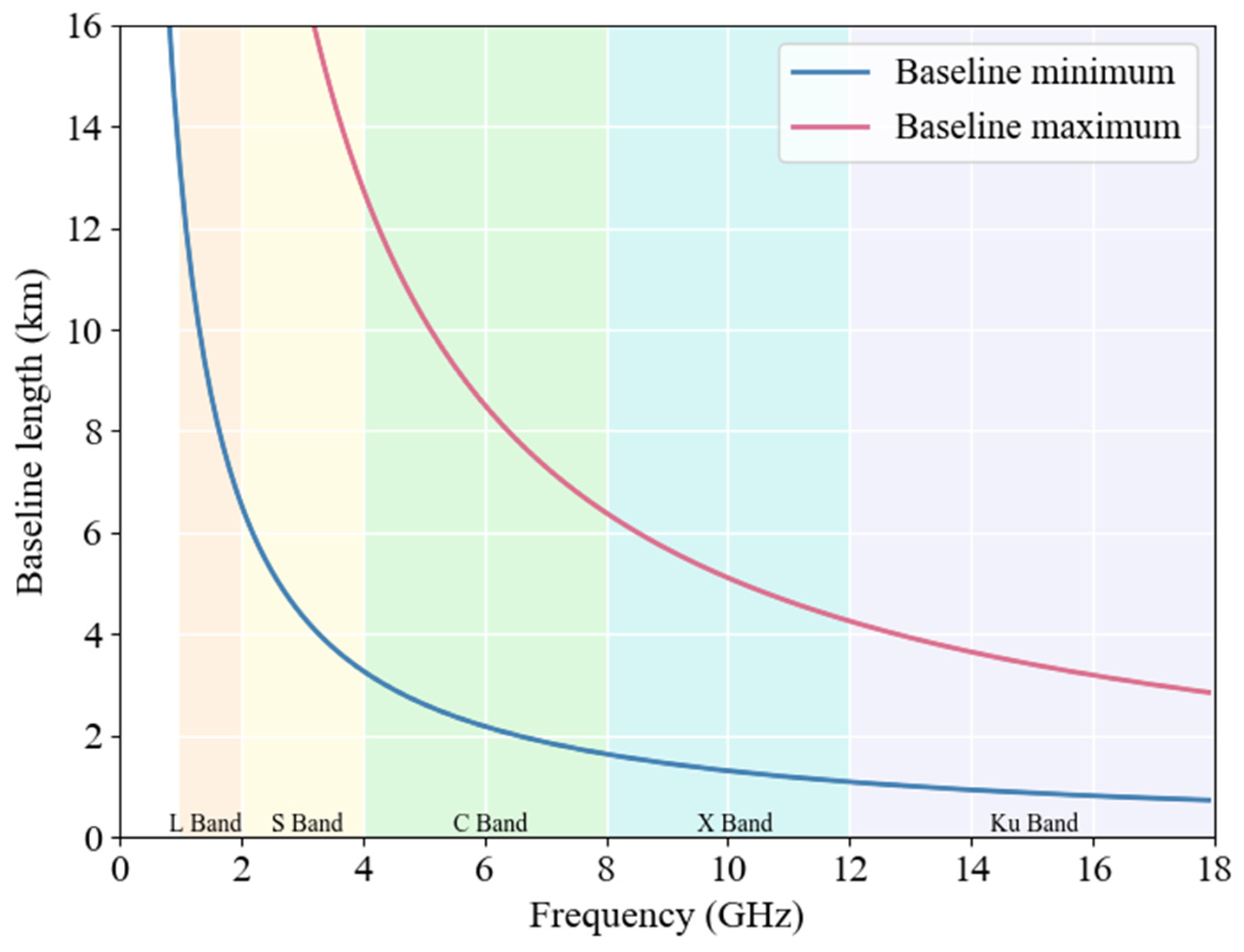
Figure 17). The red line indicates the maximum normal baseline for each frequency to avoid very low coherence, while the blue line indicates the minimum normal baseline to ensure sufficient volume sensitivity. In
Figure 17, the center frequency points of the spaceborne SAR bands (S: 3.2 GHz, C: 5.3 GHz, X: 9.6 GHz, Ku: 15 GHz), the preferred ranges of vertical spatial baseline lengths are as follows: 4.10 to 15.97 km, 2.48 to 9.64 km, 1.36 to 5.32 km, and 0.87 to 3.40 km, respectively. The minimum vertical spatial baseline for the L-band (1.2 GHz) is 10.93 km, while the maximum spatial baseline, which is excessively large (42.59 km), is not displayed in the graph. In this case, the upper limits of the baseline corresponding to the minimum coherence also correspond to a very high normal baseline, which may be completely out of coherence in reality, and the lower limit restriction of the baseline is more relevant than the upper limit.
4. Conclusions
In this study, a rice height inversion method based on the OVoG model was implemented using multi-frequency, multi-angle, and multi-baseline PolInSAR experimental data obtained from the LAMP microwave anechoic chamber. This study investigated the impact of changes in incident wave frequency, incident angle, and spatial baseline on the polarization interferometric response characteristics of rice, as well as their impact on the inversion results of rice height. Therefore, an optimal detection mode for PolInSAR interferometric measurements was proposed for rice height inversion.
The experiments demonstrate that the optimal incident angle range is 35° to 55°, with an optimal baseline length of 0.25°, yielding an RMSE of 0.1932 m and an MAE of approximately 0.1359 m, and the optimal frequency range is 4–16 GHz. For the number of baselines, a combination of 3 to 4, baselines were identified as the optimal number, with an RMSE of 0.1758 m and a MAE of approximately 0.1093 m.
Based on the equivalence of imaging geometries, the optimal spatial baseline ranges for the spaceborne SAR data on different frequency bands were: L-band: 10.93–42.59 km; S-band: 4.10–15.97 km; C-band: 2.48–9.64 km; and X-band: 1.36–5.32 km. Notably, the measurement modes corresponding to the C, X, and Ku bands were more suitable for PolInSAR rice height inversion.
Our future studies will continue to conduct theoretical and experimental research and expand the algorithm to different vegetation types. Additionally, we aim to verify the performance of the optimal detection mode by acquiring multi-temporal PolInSAR data using airborne SAR data, with the hope of providing a reliable basis for the design and preliminary research of a new generation of Earth observation SAR systems.


