
Comparison of Three Approaches for Estimating Understory Biomass in Yanshan Mountains


Abstract
:
1. Introduction
2. Materials and Methods
2.1. Study Area
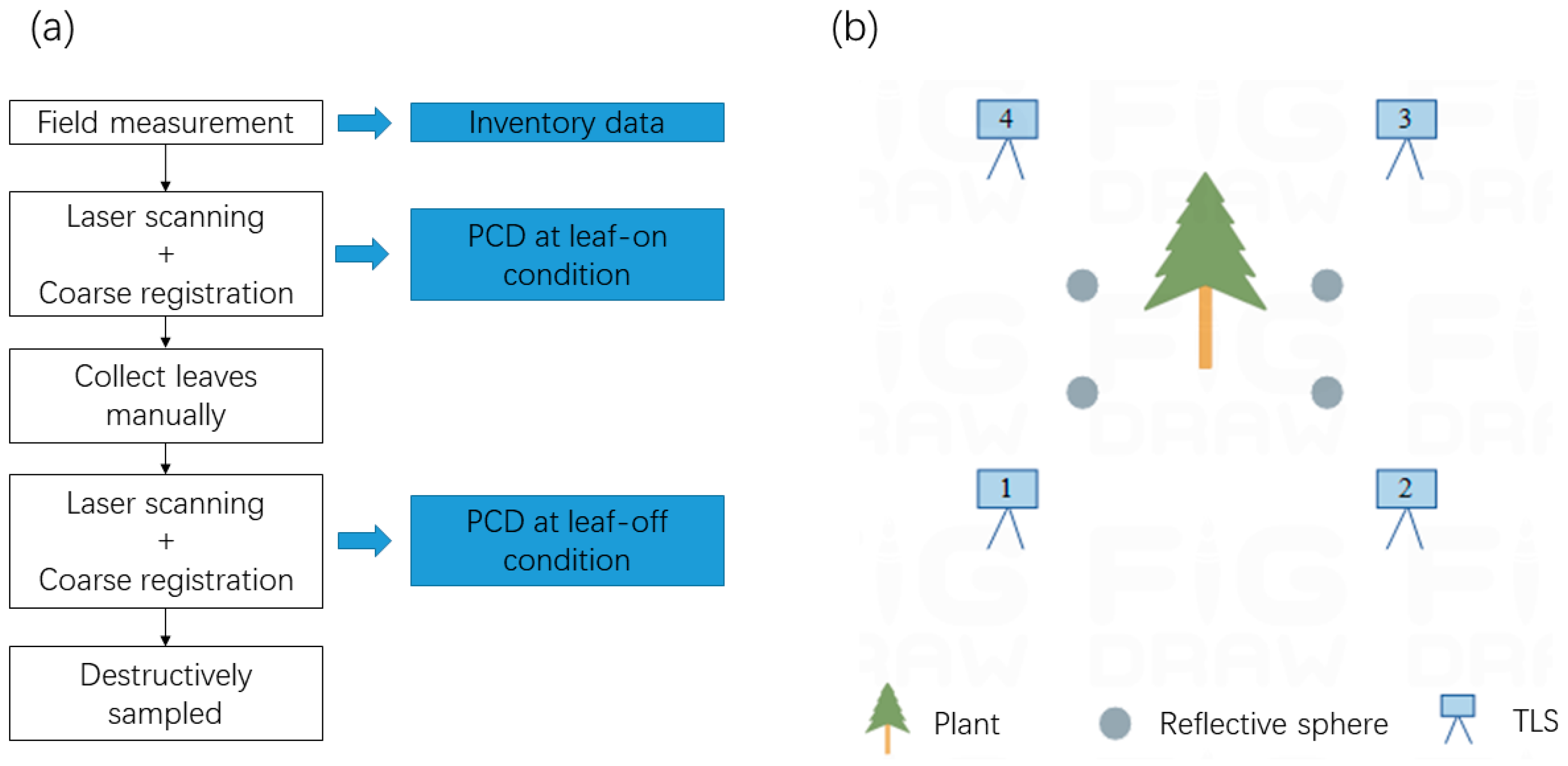
2.2. TLS and Field Data Acquisition
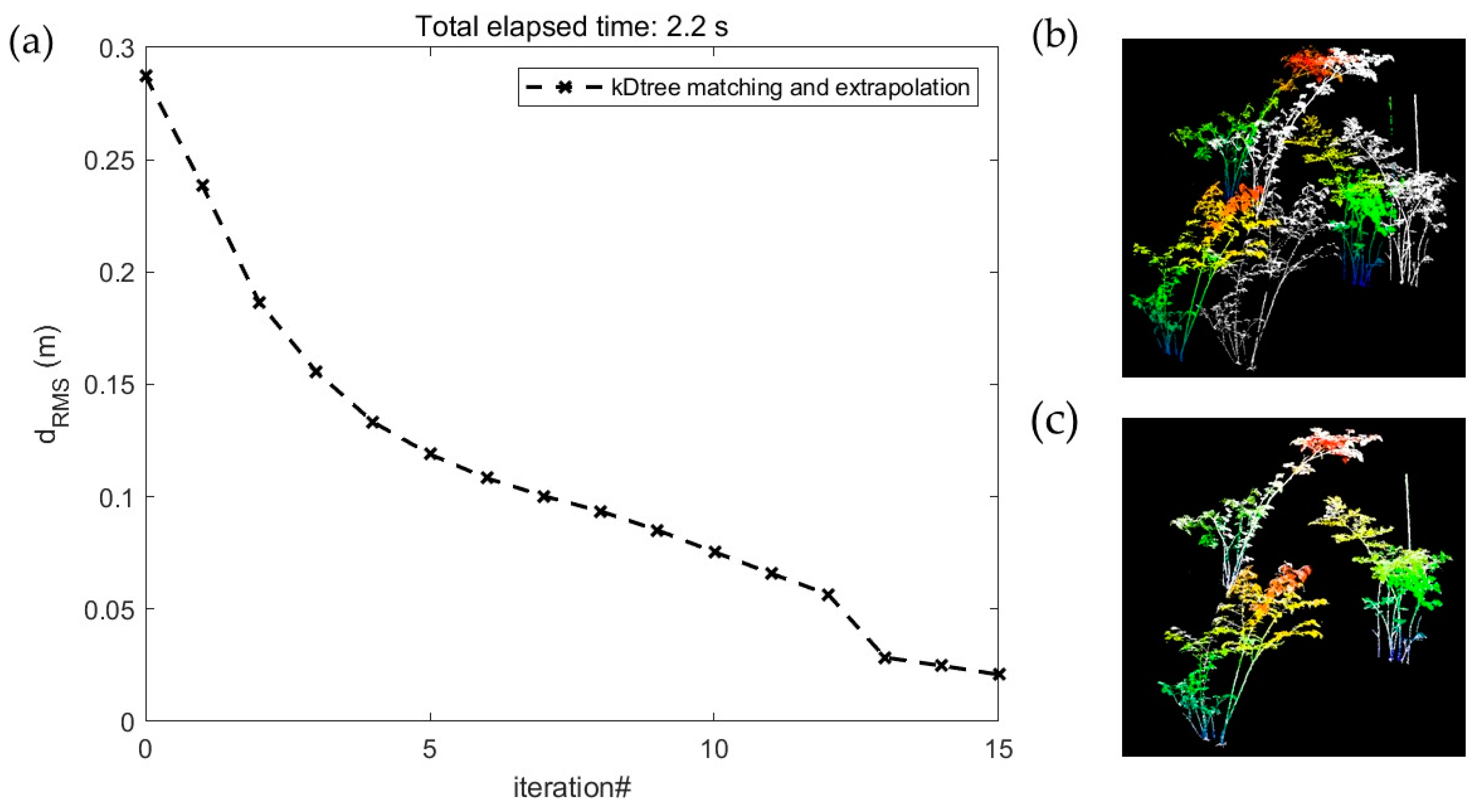
2.3. TLS Data Preprocessing
2.4. Volume and LA Calculation
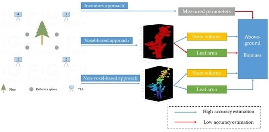
2.4.1. Method Overview
2.4.2. Volume Calculation with TLS Data
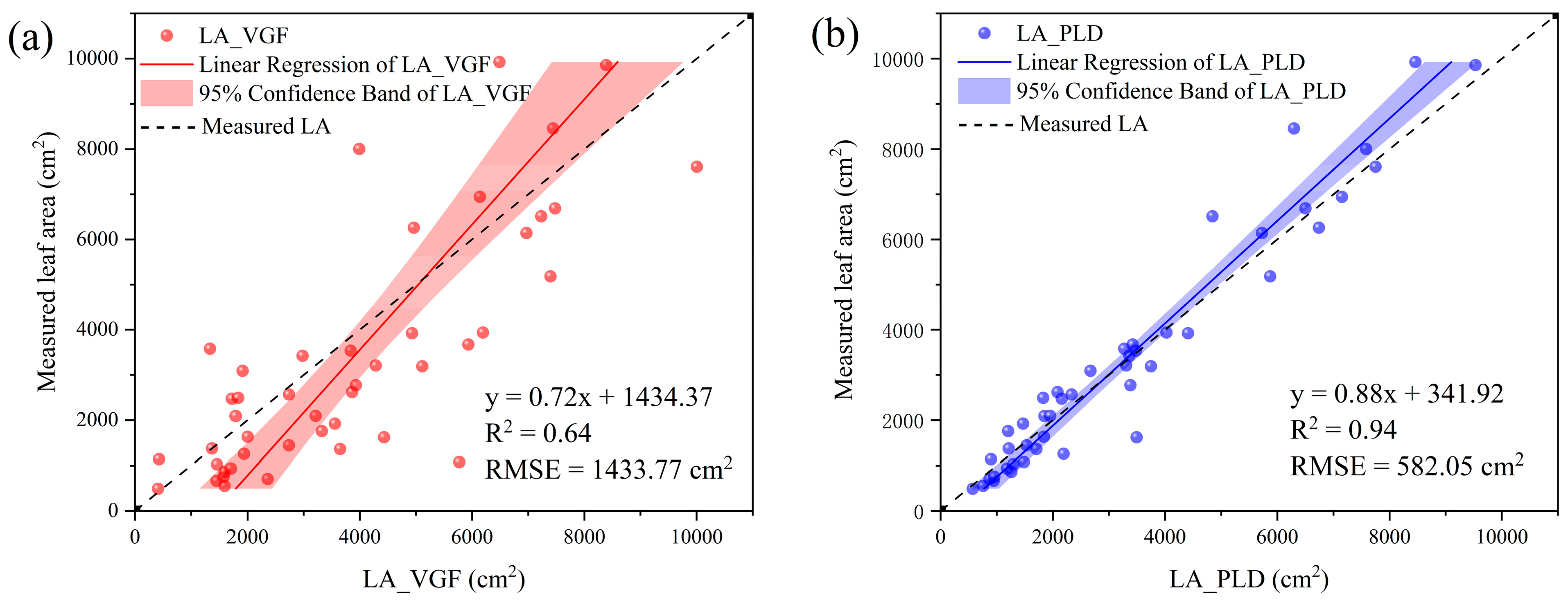
2.4.3. LA Calculation with TLS Data
2.5. Statistical Analysis
3. Results
3.1. Biomass Estimation Using Field-Measured Parameters
3.2. Biomass Estimation Using Voxelization Approaches
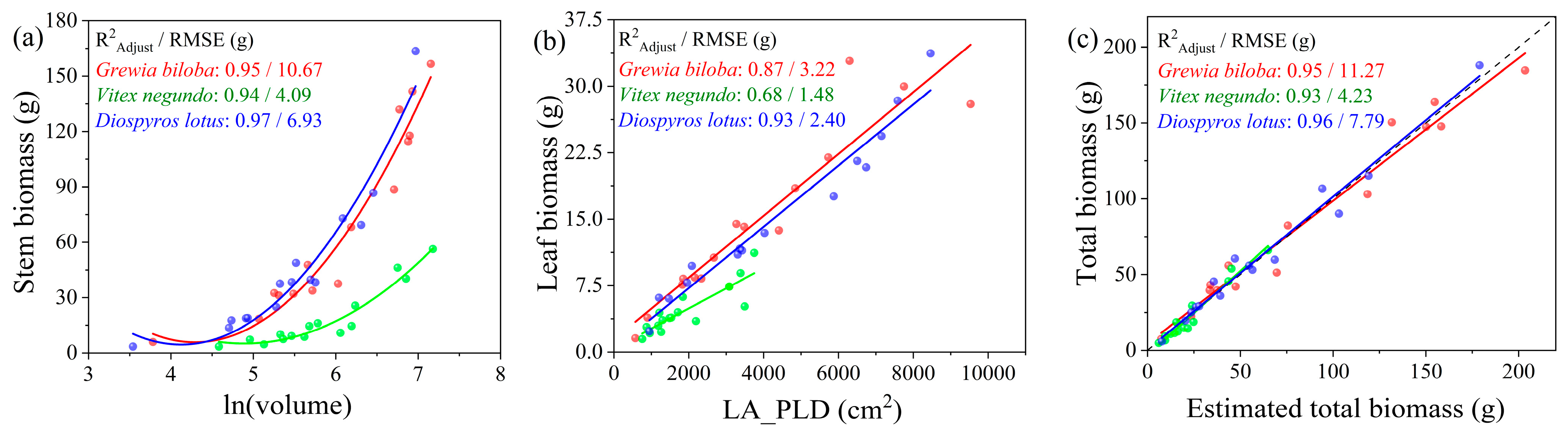
3.3. Non-Voxel-Based Approach to Estimate Leaf, Stem, and Total Biomass
3.4. Comparison of Biomass Estimation Using Inventory, Voxel-, and Non-Voxel-Based Approaches
4. Discussion
4.1. Performance of Inventory and TLS-Based Approaches
4.2. Comparison of the Voxel-Based and Non-Voxel-Based Approach
5. Conclusions
Supplementary Materials
Author Contributions
Funding
Data Availability Statement
Acknowledgments
Conflicts of Interest
References
- MacFarlane, D.W. A generalized tree component biomass model derived from principles of variable allometry. For. Ecol. Manag. 2015, 354, 43–55. [Google Scholar] [CrossRef]
- Burt, A.; Vicari, M.B.; da Costa, A.C.L.; Coughlin, I.; Rowland, L.; Disney, M. New insights into large tropical tree mass and structure from direct harvest and terrestrial lidar. R. Soc. Open Sci. 2021, 8, 201458. [Google Scholar] [CrossRef] [PubMed]
- Kukenbrink, D.; Gardi, O.; Morsdorf, F.; Thurig, E.; Schellenberger, A.; Mathys, L. Above-ground biomass references for urban trees from terrestrial laser scanning data. Ann. Bot. 2021, 128, 709–724. [Google Scholar] [CrossRef] [PubMed]
- Dixon, R.K.; Solomon, A.M.; Brown, S.; Houghton, R.A.; Trexier, M.C.; Wisniewski, J. Carbon pools and flux of global forest ecosystems. Science 1994, 263, 185–190. [Google Scholar] [CrossRef]
- Guo, Z.; Fang, J.; Pan, Y.; Birdsey, R. Inventory-based estimates of forest biomass carbon stocks in China: A comparison of three methods. For. Ecol. Manag. 2010, 259, 1225–1231. [Google Scholar] [CrossRef]
- Chambers, J.Q.; Asner, G.P.; Morton, D.C.; Anderson, L.O.; Saatch, S.S.; Espirito-Santo, F.D.B.; Palace, M.; Souza, C., Jr. Regional ecosystem structure and function: Ecological insights from remote sensing of tropical forests. Trends Ecol. Evol. 2007, 22, 414–423. [Google Scholar] [CrossRef]
- Le Noe, J.; Erb, K.-H.; Matej, S.; Magerl, A.; Bhan, M.; Gingrich, S. Altered growth conditions more than reforestation counteracted forest biomass carbon emissions 1990–2020. Nat. Commun. 2021, 12, 6075. [Google Scholar] [CrossRef]
- Yarie, J. The Role of Understory Vegetation in the Nutrient Cycle of Forested Ecosystems in the Mountain Hemlock Biogeoclimatic Zone. Ecology 1980, 61, 1498–1514. [Google Scholar] [CrossRef]
- Misson, L.; Baldocchi, D.D.; Black, T.A.; Blanken, P.D.; Brunet, Y.; Yuste, J.C.; Dorsey, J.R.; Falk, M.; Granier, A.; Irvine, M.R.; et al. Partitioning forest carbon fluxes with overstory and understory eddy-covariance measurements: A synthesis based on FLUXNET data. Agric. For. Meteorol. 2007, 144, 14–31. [Google Scholar] [CrossRef]
- Moore, P.T.; Van Miegroet, H.; Nicholas, N.S. Relative role of understory and overstory in carbon and nitrogen cycling in a southern Appalachian spruce-fir forest. Can. J. For. Res. 2007, 37, 2689–2700. [Google Scholar] [CrossRef]
- Benjamin, B.C.; Hudak, A.T.; Meddens, A.J.H.; Hawbaker, T.J.; Briggs, J.S.; Kennedy, R.E. Prediction of Forest Canopy and Surface Fuels from Lidar and Satellite Time Series Data in a Bark Beetle-Affected Forest. Forests 2017, 8, 322. [Google Scholar]
- White, J.C.; Coops, N.C.; Wulder, M.A.; Vastaranta, M.; Hilker, T.; Tompalski, P. Remote Sensing Technologies for Enhancing Forest Inventories: A Review. Can. J. Remote Sens. 2016, 42, 619–641. [Google Scholar] [CrossRef]
- Greaves, H.E.; Vierling, L.A.; Eitel, J.U.H.; Boelman, N.T.; Magney, T.S.; Prager, C.M.; Griffin, K.L. Estimating aboveground biomass and leaf area of low-stature Arctic shrubs with terrestrial LiDAR. Remote Sens. Environ. 2015, 164, 26–35. [Google Scholar] [CrossRef]
- Demol, M.; Verbeeck, H.; Gielen, B.; Armston, J.; Burt, A.; Disney, M.; Duncanson, L.; Hackenberg, J.; Kukenbrink, D.; Lau, A.; et al. Estimating forest above-ground biomass with terrestrial laser scanning: Current status and future directions. Methods Ecol. Evol. 2022, 13, 1628–1639. [Google Scholar] [CrossRef]
- Calders, K.; Newnham, G.; Burt, A.; Murphy, S.; Raumonen, P.; Herold, M.; Culvenor, D.; Avitabile, V.; Disney, M.; Armston, J.; et al. Nondestructive estimates of above-ground biomass using terrestrial laser scanning. Methods Ecol. Evol. 2015, 6, 198–208. [Google Scholar] [CrossRef]
- Huff, S.; Ritchie, M.; Temesgen, H. Allometric equations for estimating aboveground biomass for common shrubs in northeastern California. For. Ecol. Manag. 2017, 398, 48–63. [Google Scholar] [CrossRef]
- Colgan, M.S.; Asner, G.P.; Swemmer, T. Harvesting tree biomass at the stand level to assess the accuracy of field and airborne biomass estimation in savannas. Ecol. Appl. 2013, 23, 1170–1184. [Google Scholar] [CrossRef]
- Quint, T.C.; Dech, J.P. Allometric models for predicting the aboveground biomass of Canada yew (Taxus canadensis Marsh.) from visual and digital cover estimates. Can. J. For. Res. 2010, 40, 2003–2014. [Google Scholar] [CrossRef]
- Chen, Y.; Cai, X.A.; Zhang, Y.; Rao, X.; Fu, S. Dynamics of Understory Shrub Biomass in Six Young Plantations of Southern Subtropical China. Forests 2017, 8, 419. [Google Scholar] [CrossRef]
- Asner, G.P.; Mascaro, J.; Anderson, C.; Knapp, D.E.; Martin, R.E.; Kennedy-Bowdoin, T.; van Breugel, M.; Davies, S.; Hall, J.S.; Muller-Landau, H.C.; et al. High-fidelity national carbon mapping for resource management and REDD+. Carbon Balanc. Manag. 2013, 8, 7. [Google Scholar] [CrossRef]
- Du, L.; Pang, Y.; Wang, Q.; Huang, C.; Bai, Y.; Chen, D.; Lu, W.; Kong, D. A LiDAR biomass index-based approach for tree- and plot-level biomass mapping over forest farms using 3D point clouds. Remote Sens. Environ. 2023, 290, 113543. [Google Scholar] [CrossRef]
- Wang, F.; Sun, Y.; Jia, W.; Li, D.; Zhang, X.; Tang, Y.; Guo, H. A Novel Approach to Characterizing Crown Vertical Profile Shapes Using Terrestrial Laser Scanning (TLS). Remote Sens. 2023, 15, 3272. [Google Scholar] [CrossRef]
- Lefsky, M.A.; Cohen, W.B.; Harding, D.J.; Parker, G.G.; Acker, S.A.; Gower, S.T. Lidar remote sensing of above-ground biomass in three biomes. Glob. Ecol. Biogeogr. 2002, 11, 393–399. [Google Scholar] [CrossRef]
- Kato, A.; Moskal, L.M.; Schiess, P.; Swanson, M.E.; Calhoun, D.; Stuetzle, W. Capturing tree crown formation through implicit surface reconstruction using airborne lidar data. Remote Sens. Environ. 2016, 113, 1148–1162. [Google Scholar] [CrossRef]
- Drake, J.B.; Dubayah, R.O.; Clark, D.B.; Knox, R.G.; Blair, J.B.; Hofton, M.A.; Chazdon, R.L.; Weishampel, J.F.; Prince, S. Estimation of tropical forest structural characteristics using large-footprint lidar. Remote Sens. Environ. 2002, 79, 305–319. [Google Scholar] [CrossRef]
- Glenn, N.F.; Spaete, L.P.; Sankey, T.T.; Derryberry, D.R.; Hardegree, S.P.; Mitchell, J.J. Errors in LiDAR-derived shrub height and crown area on sloped terrain. J. Arid. Environ. 2011, 75, 377–382. [Google Scholar] [CrossRef]
- Mitchell, J.J.; Glenn, N.F.; Sankey, T.T.; Derryberry, D.R.; Anderson, M.O.; Hruska, R.C. Small-footprint lidar estimations of sagebrush canopy characteristics. Photogramm. Eng. Remote Sens. 2011, 77, 521–530. [Google Scholar] [CrossRef]
- Bork, E.W.; Su, J.G. Integrating LIDAR data and multispectral imagery for enhanced classification of rangeland vegetation: A meta analysis. Remote Sens. Environ. 2007, 111, 11–24. [Google Scholar] [CrossRef]
- Li, S.; Wang, T.; Hou, Z.; Gong, Y.; Feng, L.; Ge, J. Harnessing terrestrial laser scanning to predict understory biomass in temperate mixed forests. Ecol. Indic. 2021, 121, 107011. [Google Scholar] [CrossRef]
- Arseniou, G.; MacFarlane, D.W.; Calders, K.; Baker, M. Accuracy differences in aboveground woody biomass estimation with terrestrial laser scanning for trees in urban and rural forests and different leaf conditions. Trees-Struct. Funct. 2023, 37, 761–779. [Google Scholar] [CrossRef]
- Arslan, A.E.; Erten, E.; Inan, M. A comparative study for obtaining effective Leaf Area Index from single Terrestrial Laser Scans by removal of wood material. Measurement 2021, 178, 109262. [Google Scholar] [CrossRef]
- Béland, M.; Widlowski, J.-L.; Fournier, R.A.; Côté, J.-F.; Verstraete, M.M. Estimating leaf area distribution in savanna trees from terrestrial LiDAR measurements. Agric. For. Meteorol. 2011, 151, 1252–1266. [Google Scholar] [CrossRef]
- Li, S.; Dai, L.; Wang, H.; Wang, Y.; He, Z.; Lin, S. Estimating Leaf Area Density of Individual Trees Using the Point Cloud Segmentation of Terrestrial LiDAR Data and a Voxel-Based Model. Remote Sens. 2017, 9, 1202. [Google Scholar] [CrossRef]
- Nguyen, V.T.; Fournier, R.A.; Côté, J.F.; Pimont, F. Estimation of vertical plant area density from single return terrestrial laser scanning point clouds acquired in forest environments. Remote Sens. Environ. 2022, 279, 113115. [Google Scholar] [CrossRef]
- Puletti, N.; Galluzzi, M.; Grotti, M.; Ferrara, C. Characterizing subcanopy structure of Mediterranean forests by terrestrial laser scanning data. Remote Sens. Appl.-Soc. Environ. 2021, 24, 100620. [Google Scholar] [CrossRef]
- Brolly, G.; Király, G.; Lehtomäki, M.; Liang, X. Voxel-Based Automatic Tree Detection and Parameter Retrieval from Terrestrial Laser Scans for Plot-Wise Forest Inventory. Remote Sens. 2021, 13, 542. [Google Scholar] [CrossRef]
- Zheng, G.; Moskal, L.M.; Kim, S.H. Retrieval of Effective Leaf Area Index in Heterogeneous Forests with Terrestrial Laser Scanning. IEEE Trans. Geosci. Remote Sens. 2013, 51, 777–786. [Google Scholar] [CrossRef]
- Kükenbrink, D.; Schneider, F.D.; Leiterer, R.; Schaepman, M.E.; Morsdorf, F. Quantification of hidden canopy volume of airborne laser scanning data using a voxel traversal algorithm. Remote Sens. Environ. 2017, 194, 424–436. [Google Scholar] [CrossRef]
- Cifuentes, R.; Van der Zande, D.; Farifteh, J.; Salas, C.; Coppin, P. Effects of voxel size and sampling setup on the estimation of forest canopy gap fraction from terrestrial laser scanning data. Agric. For. Meteorol. 2014, 194, 230–240. [Google Scholar] [CrossRef]
- Campbell, M.J.; Dennison, P.E.; Hudak, A.T.; Parham, L.M.; Butler, B.W. Quantifying understory vegetation density using small-footprint airborne lidar. Remote Sens. Environ. 2018, 215, 330–342. [Google Scholar] [CrossRef]
- Soma, M.; Pimont, F.; Durrieu, S.; Dupuy, J.L. Enhanced Measurements of Leaf Area Density with T-LiDAR: Evaluating and Calibrating the Effects of Vegetation Heterogeneity and Scanner Properties. Remote Sens. 2018, 10, 1580. [Google Scholar] [CrossRef]
- Béland, M.; Baldocchi, D.D.; Widlowski, J.; Fournier, R.A.; Verstraete, M.M. On seeing the wood from the leaves and the role of voxel size in determining leaf area distribution of forests with terrestrial LiDAR. Agric. For. Meteorol. 2014, 184, 82–97. [Google Scholar] [CrossRef]
- Soma, M.; Pimont, F.; Dupuy, J.L. Sensitivity of voxel-based estimations of leaf area density with terrestrial LiDAR to vegetation structure and sampling limitations: A simulation experiment. Remote Sens. Environ. 2021, 257, 112354. [Google Scholar] [CrossRef]
- Menéndez-Miguélez, M.; Madrigal, G.; Sixto, H.; Oliveira, N.; Calama, R. Terrestrial Laser Scanning for Non-Destructive Estimation of Aboveground Biomass in Short-Rotation Poplar Coppices. Remote Sens. 2023, 15, 1942. [Google Scholar] [CrossRef]
- Yao, X.; Yang, G.; Wu, B.; Jiang, L.; Wang, F. Biomass Estimation Models for Six Shrub Species in Hunshandake Sandy Land in Inner Mongolia, Northern China. Forests 2021, 12, 167. [Google Scholar] [CrossRef]
- Besl, P.J.; Mckay, H.D. A method for registration of 3-D shapes. IEEE Trans. Pattern Anal. Mach. Intell. 1992, 14, 239–256. [Google Scholar] [CrossRef]
- Loudermilk, E.L.; Hiers, J.K.; O’Brien, J.J.; Mitchell, R.J.; Singhanaia, A.; Fernandez, J.C.; Cropper, W.P., Jr.; Slatton, K.C. Ground-based LIDAR: A novel approach to quantify fine-scale fuelbed characteristics. Int. J. Wildland Fire 2009, 18, 676–685. [Google Scholar] [CrossRef]
- Hosoi, F.; Omasa, K. Voxel-Based 3-D Modeling of Individual Trees for Estimating Leaf Area Density Using High-Resolution Portable Scanning Lidar. IEEE Trans. Geosci. Remote Sens. 2006, 44, 3610–3618. [Google Scholar] [CrossRef]
- Liu, X.; Wang, Y.; Kang, F.; Yue, Y.; Zheng, Y. Canopy Parameter Estimation of Citrus grandis var. Longanyou Based on LiDAR 3D Point Clouds. Remote Sens. 2021, 13, 1859. [Google Scholar] [CrossRef]
- Di Gennaro, S.F.; Matese, A. Evaluation of novel precision viticulture tool for canopy biomass estimation and missing plant detection based on 2.5D and 3D approaches using RGB images acquired by UAV platform. Plant Methods 2020, 16, 91. [Google Scholar] [CrossRef]
- Zhu, T.; Ma, X.; Guan, H.; Wu, X.; Wang, F.; Yang, C.; Jiang, Q. A calculation method of phenotypic traits based on three-dimensional reconstruction of tomato canopy. Comput. Electron. Agric. 2023, 204, 107515. [Google Scholar] [CrossRef]
- Monsi, M.; Saeki, T. On the Factor Light in Plant Communities and its Importance for Matter Production. Ann. Bot. 2005, 95, 549–567. [Google Scholar] [CrossRef] [PubMed]
- Yan, G.; Hu, R.; Luo, J.; Weiss, M.; Jiang, H.; Mu, X.; Xie, D.; Zhang, W. Review of indirect optical measurements of leaf area index: Recent advances, challenges, and perspectives. Agric. For. Meteorol. 2019, 265, 390–411. [Google Scholar] [CrossRef]
- Asner, G.P.; Scurlock, J.M.O.; Hicke, J.A. Global synthesis of leaf area index observations: Implications for ecological and remote sensing studies. Glob. Ecol. Biogeogr. 2003, 12, 191–205. [Google Scholar] [CrossRef]
- Welles, J.M.; Cohen, S. Canopy structure measurement by gap fraction analysis using commercial instrumentation. J. Exp. Bot. 1996, 47, 1335–1342. [Google Scholar] [CrossRef]
- Hu, R.; Bournez, E.; Cheng, S.; Jiang, H.; Nerry, F.; Landes, T.; Saudreau, M.; Kastendeuch, P.; Najjar, G.; Colin, J.; et al. Estimating the leaf area of an individual tree in urban areas using terrestrial laser scanner and path length distribution model. ISPRS-J. Photogramm. Remote Sens. 2018, 144, 357–368. [Google Scholar] [CrossRef]
- Liu, Z.; Chen, R.; Song, Y.; Han, C.; Yang, Y. Estimation of aboveground biomass for alpine shrubs in the upper reaches of the Heihe River Basin, Northwestern China. Environ. Earth Sci. 2015, 73, 5513–5521. [Google Scholar] [CrossRef]
- Elzein, T.M.; Blarquez, O.; Gauthier, O.; Carcaillet, C. Allometric equations for biomass assessment of subalpine dwarf shrubs. Alp. Bot. 2011, 121, 129–134. [Google Scholar] [CrossRef]
- Dahlberg, U.; Berge, T.W.; Petersson, H.; Vencatasawmy, C.P. Modelling biomass and leaf area index in a sub-arctic Scandinavian mountain area. Scand. J. For. Res. 2007, 19, 60–71. [Google Scholar] [CrossRef]
- Kuyah, S.; Muthuri, C.; Jamnadass, R.; Mwangi, P.; Neufeldt, H.; Dietz, J. Crown area allometries for estimation of aboveground tree biomass in agricultural landscapes of western Kenya. Agrofor. Syst. 2012, 86, 267–277. [Google Scholar] [CrossRef]
- Kalita, R.M.; Das, A.K.; Nath, A.J. Allometric equations for estimating above- and belowground biomass in Tea (Camellia sinensis (L.) O. Kuntze) agroforestry system of Barak Valley, Assam, northeast India. Biomass Bioenerg. 2015, 83, 42–49. [Google Scholar] [CrossRef]
- Flade, L.; Hopkinson, C.; Chasmer, L. Allometric Equations for Shrub and Short-Stature Tree Aboveground Biomass within Boreal Ecosystems of Northwestern Canada. Forests 2020, 11, 1207. [Google Scholar] [CrossRef]
- Zong, X.; Wang, T.; Skidmore, A.K.; Heurich, M. The impact of voxel size, forest type, and understory cover on visibility estimation in forests using terrestrial laser scanning. GISci. Remote Sens. 2021, 58, 323–339. [Google Scholar] [CrossRef]
- Weiser, H.; Winiwarter, L.; Anders, K.; Fassnacht, F.E.; Hoefle, B. Opaque voxel-based tree models for virtual laser scanning in forestry applications. Remote Sens. Environ. 2021, 265, 112641. [Google Scholar] [CrossRef]
- Chen, J.M.; Mo, G.; Pisek, J.; Liu, J.; Deng, F.; Ishizawa, M.; Chan, D. Effects of foliage clumping on the estimation of global terrestrial gross primary productivity. Glob. Biogeochem. Cycle 2012, 26, GB1019. [Google Scholar] [CrossRef]
- Zou, J.; Yan, G.; Chen, L. Estimation of Canopy and Woody Components Clumping Indices at Three Mature Picea crassifolia Forest Stands. IEEE J. Sel. Top. Appl. Earth Observ. Remote Sens. 2015, 8, 1413–1422. [Google Scholar] [CrossRef]
- Hu, R.; Yan, G.; Mu, X.; Luo, J. Indirect measurement of leaf area index on the basis of path length distribution. Remote Sens. Environ. 2014, 155, 239–247. [Google Scholar] [CrossRef]
- Korhonen, L.; Vauhkonen, J.; Virolainen, A.; Hovi, A.; Korpela, I. Estimation of tree crown volume from airborne lidar data using computational geometry. Int. J. Remote Sens. 2013, 34, 7236–7248. [Google Scholar] [CrossRef]
- Li, Q.; Gao, X.; Fei, X.; Zhang, H.; Wang, J.; Cui, Y.; Li, B. Construction of Tree Crown Three-dimensional Model Using Alpha-shape Algorithm. Bull. Surv. Mapp. 2018, 12, 91–95. [Google Scholar]
- Olsoy, P.J.; Mitchell, J.J.; Levia, D.F.; Clark, P.E.; Glenn, N.F. Estimation of big sagebrush leaf area index with terrestrial laser scanning. Ecol. Indic. 2016, 61, 815–821. [Google Scholar] [CrossRef]
- Martin-Ducup, O.; Robert, S.; Fournier, R.A. A method to quantify canopy changes using multi-temporal terrestrial lidar data: Tree response to surrounding gaps. Agric. For. Meteorol. 2017, 237, 184–195. [Google Scholar]
- Latella, M.; Raimondo, T.; Belcore, E.; Salerno, L.; Camporeale, C. On the integration of LiDAR and field data for riparian biomass estimation. J. Environ. Manag. 2022, 322, 116046. [Google Scholar] [CrossRef]
- Domingo, D.; Luis Montealegre, A.; Teresa Lamelas, M.; Garcia-Martin, A.; de la Riva, J.; Rodriguez, F.; Alonso, R. Quantifying forest residual biomass in Pinus halepensis Miller stands using Airborne Laser Scanning data. GISci. Remote Sens. 2019, 56, 1210–1232. [Google Scholar] [CrossRef]
- Domingo, D.; Teresa Lamelas, M.; Luis Montealegre, A.; Garcia-Martin, A.; de la Riva, J. Estimation of Total Biomass in Aleppo Pine Forest Stands Applying Parametric and Nonparametric Methods to Low-Density Airborne Laser Scanning Data. Forests 2018, 9, 158. [Google Scholar] [CrossRef]
- Sackov, I.; Barka, I.; Bucha, T. Mapping Aboveground Woody Biomass on Abandoned Agricultural Land Based on Airborne Laser Scanning Data. Remote Sens. 2021, 12, 4189. [Google Scholar] [CrossRef]
- De Frenne, P.; Rodríguez-Sánchez, F.; De Schrijver, A.; Coomes, D.A.; Hermy, M.; Vangansbeke, P.; Verheyen, K. Light accelerates plant responses to warming. Nat. Plants 2015, 1, 15110. [Google Scholar] [CrossRef]
- Verheyen, K.; Baeten, L.; De Frenne, P.; Bernhardt-RoeMermann, M.; Brunet, J.; Cornelis, J.; Decocq, G.; Dierschke, H.; Eriksson, O.; Hédl, R. Driving factors behind the eutrophication signal in understorey plant communities of deciduous temperate forests. J. Ecol. 2012, 100, 352–365. [Google Scholar] [CrossRef]
- Landuyt, D.; Maes, S.L.; Depauw, L.; Ampoorter, E.; Blondeel, H.; Perring, M.P.; Brumelis, G.; Brunet, J.; Decocq, G.; den Ouden, J.; et al. Drivers of above-ground understorey biomass and nutrient stocks in temperate deciduous forests. J. Ecol. 2019, 108, 982–997. [Google Scholar] [CrossRef]
- Beets, P.N.; Kimberley, M.O.; Oliver, G.R.; Pearce, S.H. The Application of Stem Analysis Methods to Estimate Carbon Sequestration in Arboreal Shrubs from a Single Measurement of Field Plots. Forests 2014, 5, 919–935. [Google Scholar] [CrossRef]
- Berner, L.T.; Jantz, P.; Tape, K.D.; Goetz, S.J. Tundra plant above-ground biomass and shrub dominance mapped across the North Slope of Alaska. Environ. Res. Lett. 2018, 13, 035002. [Google Scholar] [CrossRef]


| Attribute | Specification |
|---|---|
| Wavelength | 1550 nm, invisible |
| Field of View | 360° (horizontal) × 282° (vertical) |
| Scanning Frequency | >500 kHZ |
| Range | 0.6 m–80 m |
| Range Accuracy | 2 mm |
| Angular Accuracy | 21″ |
| 3D Point Accuracy | 2.4 mm at 10 m, 3.5 mm at 20 m, 6.0 mm at 40 m |
| Species | Measured Biomass | Parameters | R2, R2Adjusted | RMSE (g) | rRMSE % | p-Value |
|---|---|---|---|---|---|---|
| Grewia biloba | Total biomass | Crown Area | 0.61, 0.58 | 38.11 | 44.62 | <0.001 |
| n = 15 | Crown Length | 0.51, 0.48 | 42.46 | 49.71 | 0.003 | |
| OLS regression | Crown Width | 0.61, 0.58 | 38.09 | 44.60 | <0.001 | |
| Height | 0.80, 0.79 | 26.93 | 31.53 | <0.001 | ||
| Basal Diameter | 0.25, 0.19 | 52.61 | 61.60 | 0.056 | ||
| NLS regression | Basal Diameter, height | 0.32, 0.26 | 50.30 | 58.89 | 0.029 | |
| Crown Area | 0.61, 0.68 | 35.49 | 41.55 | <0.001 | ||
| Vitex negundo | Total biomass | Crown Area | 0.47, 0.42 | 14.18 | 62.03 | 0.005 |
| n = 15 | Crown Length | 0.57, 0.54 | 12.67 | 55.42 | <0.001 | |
| OLS regression | Crown Width | 0.27, 0.21 | 16.62 | 72.70 | 0.045 | |
| Height | 0.63, 0.61 | 11.76 | 51.44 | <0.001 | ||
| Basal Diameter | 0.11, 0.04 | 18.39 | 80.44 | 0.229 | ||
| NLS regression | Basal Diameter, height | 0.10, 0.03 | 18.52 | 81.01 | 0.258 | |
| Crown Area | 0.48, 0.44 | 14.97 | 65.49 | 0.004 | ||
| Diospyros lotus | Total biomass | Crown Area | 0.88, 0.87 | 16.61 | 27.11 | <0.001 |
| n = 15 | Crown Length | 0.76, 0.74 | 23.74 | 38.74 | <0.001 | |
| OLS regression | Crown Width | 0.75, 0.73 | 24.03 | 39.22 | <0.001 | |
| Height | 0.83, 0.81 | 12.50 | 20.40 | <0.001 | ||
| Basal Diameter | 0.11, 0.04 | 46.16 | 75.34 | 0.231 | ||
| NLS regression | Basal Diameter, height | 0.09, 0.02 | 46.70 | 76.22 | 0.288 | |
| Crown Area | 0.91, 0.90 | 12.38 | 20.21 | <0.001 |
| Species | Measured Biomass | Parameters | R2, Adjusted R2 | RMSE (g) | rRMSE % | p-Value |
|---|---|---|---|---|---|---|
| Grewia biloba | Total biomass | Plant volume | 0.87, 0.86 | 19.16 | 22.43 | <0.001 |
| n = 15 | Leaf biomass | LA | 0.86, 0.85 | 3.76 | 25.37 | <0.001 |
| Stem biomass | Stem volume | 0.89, 0.87 | 17.62 | 24.96 | <0.001 | |
| Total biomass | Stem volume, LA | 0.91, 0.90 | 18.18 | 21.29 | <0.001 | |
| Vitex negundo | Total biomass | Plant volume | 0.86, 0.84 | 6.43 | 28.13 | <0.001 |
| n = 15 | Leaf biomass | LA | 0.65, 0.57 | 1.82 | 40.80 | 0.014 |
| Stem biomass | Stem volume | 0.82, 0.79 | 7.37 | 40.05 | <0.001 | |
| Total biomass | Stem volume, LA | 0.86, 0.85 | 7.76 | 33.94 | <0.001 | |
| Diospyros lotus | Total biomass | Plant volume | 0.93, 0.92 | 21.03 | 34.32 | <0.001 |
| n = 15 | Leaf biomass | LA | 0.57, 0.50 | 6.36 | 42.19 | 0.013 |
| Stem biomass | Stem volume | 0.93, 0.92 | 11.06 | 23.94 | <0.001 | |
| Total biomass | Stem volume, LA | 0.96, 0.94 | 11.92 | 19.45 | <0.001 |
| Species | Parameters | Validation Method | RMSE (g) | rRMSE% | R2 | MAE (g) |
|---|---|---|---|---|---|---|
| Grewia biloba | Stem biomass and volume | LOOCV | 11.22 | 15.90 | 0.95 | 9.23 |
| Vitex negundo | 4.42 | 24.02 | 0.92 | 3.47 | ||
| Diospyros lotus | 8.15 | 17.64 | 0.96 | 6.50 |
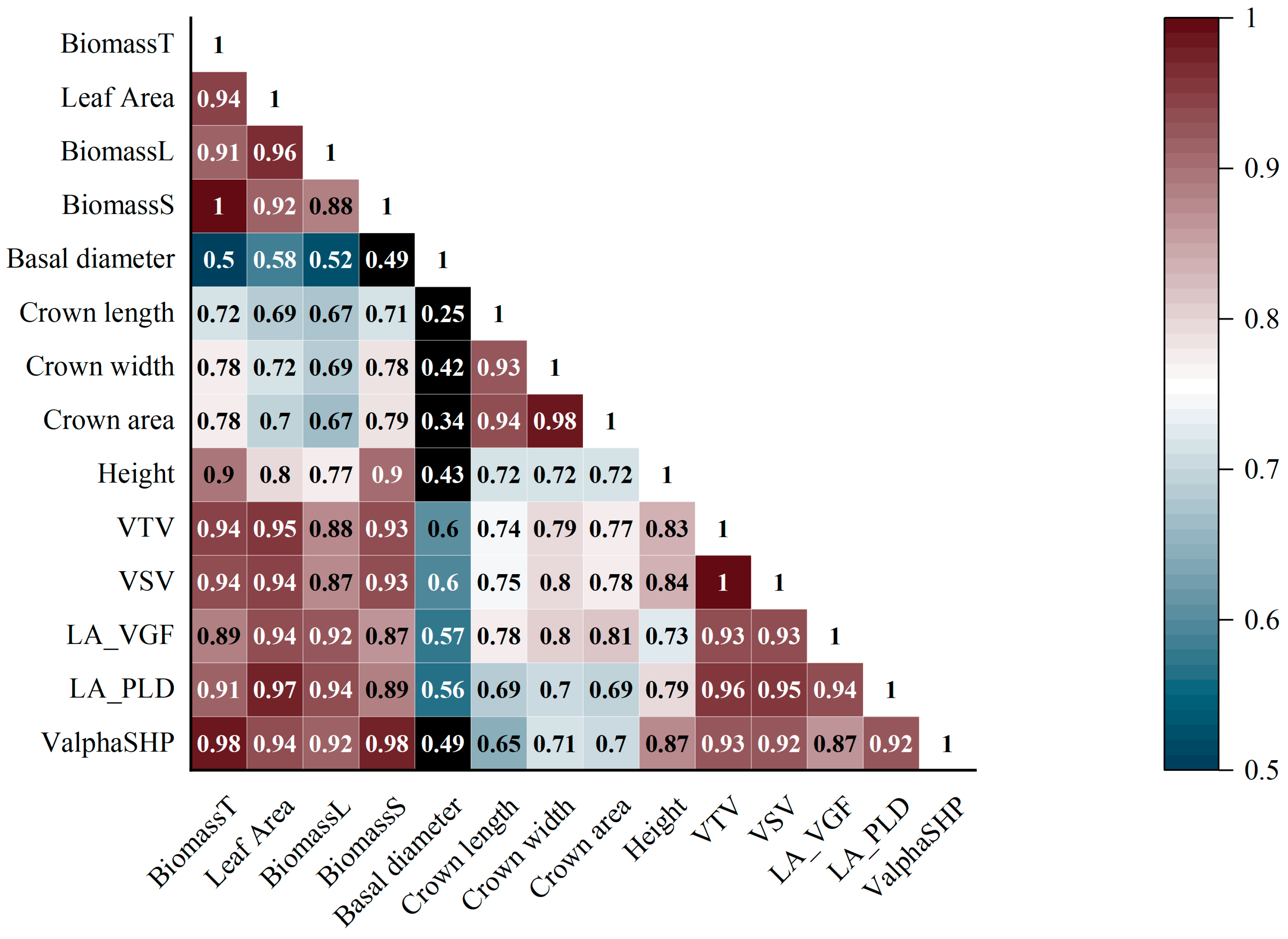
| Abbreviation | Elaboration |
|---|---|
| BiomassT, BiomassL, BiomassS | Measured total, leaf, and stem biomass |
| VTV, VSV | Total and stem volume derived from voxels |
| LA_VGF, LA_PLD | Leaf area estimated from voxels and path length distribution method |
| ValphaSHP | Stem volume derived from AS algorithms |
Disclaimer/Publisher’s Note: The statements, opinions and data contained in all publications are solely those of the individual author(s) and contributor(s) and not of MDPI and/or the editor(s). MDPI and/or the editor(s) disclaim responsibility for any injury to people or property resulting from any ideas, methods, instructions or products referred to in the content. |
© 2024 by the authors. Licensee MDPI, Basel, Switzerland. This article is an open access article distributed under the terms and conditions of the Creative Commons Attribution (CC BY) license (https://creativecommons.org/licenses/by/4.0/).
Share and Cite
Li, Y.; Hu, R.; Xing, Y.; Pang, Z.; Chen, Z.; Niu, H. Comparison of Three Approaches for Estimating Understory Biomass in Yanshan Mountains. Remote Sens. 2024, 16, 1060. https://doi.org/10.3390/rs16061060
Li Y, Hu R, Xing Y, Pang Z, Chen Z, Niu H. Comparison of Three Approaches for Estimating Understory Biomass in Yanshan Mountains. Remote Sensing. 2024; 16(6):1060. https://doi.org/10.3390/rs16061060
Chicago/Turabian StyleLi, Yuanqi, Ronghai Hu, Yuzhen Xing, Zhe Pang, Zhi Chen, and Haishan Niu. 2024. "Comparison of Three Approaches for Estimating Understory Biomass in Yanshan Mountains" Remote Sensing 16, no. 6: 1060. https://doi.org/10.3390/rs16061060