Article

Cropland and Crop Type Classification with Sentinel-1 and Sentinel-2 Time Series Using Google Earth Engine for Agricultural Monitoring in Ethiopia

1
German Remote Sensing Data Center (DFD), German Aerospace Center (DLR), 82234 Wessling, Germany
2
Department of Geography, RWTH Aachen University, 52062 Aachen, Germany
3
Deutsche Gesellschaft für Internationale Zusammenarbeit (GIZ) GmbH, Addis Ababa P.O. Box 100 009, Ethiopia
*
Author to whom correspondence should be addressed.
Remote Sens. 2024, 16(5), 866; https://doi.org/10.3390/rs16050866
Submission received: 21 December 2023 / Revised: 22 February 2024 / Accepted: 27 February 2024 / Published: 29 February 2024
(This article belongs to the Special Issue Remote Sensing Applications for the Biosphere)

Abstract

:
Cropland monitoring is important for ensuring food security in the context of global climate change and population growth. Freely available satellite data allow for the monitoring of large areas, while cloud-processing platforms enable a wide user community to apply remote sensing techniques. Remote sensing-based estimates of cropped area and crop types can thus assist sustainable land management in developing countries such as Ethiopia. In this study, we developed a method for cropland and crop type classification based on Sentinel-1 and Sentinel-2 time-series data using Google Earth Engine. Field data on 18 different crop types from three study areas in Ethiopia were available as reference for the years 2021 and 2022. First, a land use/land cover classification was performed to identify cropland areas. We then evaluated different input parameters derived from Sentinel-2 and Sentinel-1, and combinations thereof, for crop type classification. We assessed the accuracy and robustness of 33 supervised random forest models for classifying crop types for three study areas and two years. Our results showed that classification accuracies were highest when Sentinel-2 spectral bands were included. The addition of Sentinel-1 parameters only slightly improved the accuracy compared to Sentinel-2 parameters alone. The variant including S2 bands, EVI2, and NDRe2 from Sentinel-2 and VV, VH, and Diff from Sentinel-1 was finally applied for crop type classification. Investigation results of class-specific accuracies reinforced the importance of sufficient reference sample availability. The developed methods and classification results can assist regional experts in Ethiopia to support agricultural monitoring and land management.

1. Introduction

Crop type maps provide essential information for planning and decision-making in the field of agriculture and environment. Knowledge on the annual area and distribution of crops is fundamental, especially for sub-Saharan African countries that experience climate change and recurrent food insecurity. One of these countries is Ethiopia, where in 2020–2022, 26.4 million people were still undernourished according to the FAO, even though yields have increased [1] and the country has significantly improved its food systems in the past years [2]. Around 40% of the land is used for agriculture [1], and approximately 90% of the cropland is used for smallholder farming which is an important pillar of economy and people’s livelihood [2]. Several challenges for the Ethiopian food system have been formulated by the Climate Resilient Food Systems Alliance, including a lack of crop production diversity, agricultural intensification with negative effects on deforestation, soil quality, erosion, biodiversity, and water availability, as well as weak land management practices and high land fragmentation [2].
In response to current food insecurity and considerable food deficits, the government of Ethiopia strives to increase agricultural production and its efficiency [3]. Therefore, Ethiopia has been promoting large-scale agricultural investment (LSAI) to transform the agricultural sector. Three million hectares of land suitable for commercial agricultural investment have been identified, especially in lowland regions [3]. However, progress has been hindered as investors only developed a small fraction of the transferred land, due to weak institutional and legal frameworks coupled with limited capacities [3]. Therefore, there is a great need for monitoring the implementation and actual state of land use of every LSAI area. Regarding these challenges, detailed annual crop type maps could be one element to support informed agricultural and environmental decision-making as well as land management planning. But despite their importance, such datasets are not available for Ethiopia.
Earth observation allows for the derivation of such crop type maps and remote sensing has become a valuable tool for cropland and crop type mapping in recent decades [4]. Advantages of remote sensing include the repeated data collection, the applicability on a range of spatial scales, relatively low costs compared to extensive land surveys, and the possibility to map and monitor land areas that cannot be accessed by survey crews on the ground [4]. Especially since the availability of open-source remote sensing data with high spatial resolution and short revisit times, as provided by the Sentinel-1 and Sentinel-2 satellites, a valuable database for mapping cropland and crop types is available. These data provide information on crop phenology on a field scale with sufficient temporal and spatial resolution to also map smallholder farming areas.
Several approaches exist, which have been applied worldwide for crop type mapping using different databases and methods. Remote sensing approaches for crop monitoring often make use of spectral bands from multispectral satellites, such as from Sentinel-2, and vegetation indices derived thereof, which are useful for assessing the condition of vegetation [5,6,7]. Optical and NIR bands are most widely used, but red-edge bands, which are related to the physical–chemical parameters of plants, and SWIR bands, which are less affected by atmosphere scattering, have also proven useful for crop classification [8,9]. The analysis of time series is especially useful, as it provides information about plant phenology (e.g., [10]). Information derived from SAR sensors, such as from Sentinel-1, can assist crop monitoring (e.g., [11,12]), especially in cloud-prone areas. Both the backscattering coefficients of different polarization modes, as well as derivatives and radar vegetation indices derived thereof have been used in the context of crop classification [5,12,13,14]. In recent years, several studies worldwide have made use of approaches that combine optical and SAR data (e.g., [5,15,16,17,18,19,20,21]).
Methods recently applied to crop type classification include mostly machine learning algorithms, such as support vector machines, random forest, and artificial neural networks (e.g., [15,20,22]). Random forest and other decision tree models especially are widely used (e.g., [23,24,25]). These state-of-the-art classifiers are less susceptible to high-dimensional feature spaces compared to earlier methods such as parametric maximum likelihood classifiers [16]. Recent investigations were also made on unsupervised or semi-supervised classification methods for crop type classification [26,27] and towards early-season crop type mapping (e.g., [28,29,30]). A further development in recent years has shown an extended use of cloud-processing environments, such as Google Earth Engine (GEE), for remote sensing analyses, also in the context of crop classification (e.g., [23,29,31,32]). GEE was introduced in the 2010s to enhance the usability of satellite imagery for large-scale applications. The web-based platform provides earth observational data at global scale and the cloud-computing infrastructure for their analysis [33].
For Ethiopia, some studies have been published on local to regional land use/land cover mapping and change detection for selected areas within Ethiopia [34,35,36,37,38,39,40,41,42,43,44,45,46], but only a few remote sensing-based studies focused on cropland mapping or crop type classification. In the field of cropland area estimation, some research has been conducted for different regions within Ethiopia, mostly based on optical imagery. In most studies, Landsat data have been used [47,48,49], sometimes in combination with other remote sensing imagery such as IKONOS, Worldview, SPOT PROBA-V, and SRTM DEM data [50,51,52]. Other studies applied imagery from WorldView [53] and black and white photography [54]. Methods applied included logistic regression [50], supervised maximum likelihood classification [49], generalized additive models [52], object-based analyses [53], and random-forest algorithms [54].
With regard to crop type classification, studies for Ethiopia are scarce. Two studies have been published that focus on mapping the distribution of a specific crop type in Ethiopia. The first study from Guo [4] reported about mapping teff in Ethiopia. The research focused on producing a teff distribution map using satellite imagery and household data. This study made use of MODIS NDVI time series. A second study by Sahle et al. [55] focused on mapping the supply and demand of enset crop in the Wabe River catchment in southern Ethiopia. For this study, enset crop farms were digitized based on Google Earth imagery. According to our literature search, no further remote sensing-based studies on crop type differentiation in Ethiopia have been published so far.
For other regions in Sub-Saharan Africa, some studies on crop type classification and resulting crop type maps have been published, for example for South Africa [56,57], Kenya [58,59], Kenya and Tanzania [32], Benin [60], Burkina Faso [61], Ghana and Burkina Faso [62], Mali [63,64], and Madagascar [65]. In the context of the G20 Global Agriculture Monitoring Program (GEOGLAM), a harmonized, up-to-date global crop type map was developed as a set of Best Available Crop-Specific masks [66]. This product currently provides percent per pixel at 0.05 degrees for five crop types (maize, soy bean, rice, winter wheat, and spring wheat), and thus does not provide the level of detail as envisaged for this study.
In the context of lacking information on cropland area and crop type maps for Ethiopia and the need for improved monitoring of agricultural investment areas, the aim of the presented study was to develop a remote sensing-based method with the purpose of examining the land used for agricultural production and to differentiate crop types grown for LSAI areas within three regions in Ethiopia. For these areas, such information has not been available before. With respect to method development, the objective was to develop a classification method based on open-source remote sensing data implemented in a cloud-processing environment to allow for a low-threshold application by regional experts. Innovation points of the study include the classification of cultivated areas in a region where detailed land use/land cover (LULC) maps are not yet available, and the systematic analysis of satellite data input parameters for crop type classification with a large number of crop types and for six classification scenarios. Specific research questions addressed include the following: (1) What share of LSAI areas is actually used as cropland? (2) How do different combinations of input parameters derived from Sentinel-1 and Sentinel-2 data perform for crop type classification? (3) Which crop types are grown in the three study areas and what are the crop-specific classification accuracies?

2. Materials and Methods

2.1. Study Areas

The study covers three areas within the regions of Amhara, Benishangul-Gumuz, and Gambela, which are located in western Ethiopia. The study areas were defined as contiguous areas around the large-scale agricultural investment (LSAI) areas with a buffer zone of 5 km. The size of the study areas was about 1594 km2 for Amhara, 5243 km2 for Benishangul, and 6206 km2 for Gambela. Figure 1 provides an overview of the location of the study areas, their topography [67], and characteristic climate diagrams [68]. Major characteristics of the three study areas are also summarized in Table 1.
The study areas are characterized by a similar climate regime with a pronounced raining season from May through October. Temperatures generally show little variance throughout the year, but differ between study areas (19.5 °C for Amhara, 22.6 °C for Benishangul, and 27.6 °C for Gambela) in accordance with differences in terrain elevation. Gambela is the most low-lying study area with relatively flat terrain. The LSAI areas are mainly located at terrain heights between 400 m and 600 m. The Benishangul study area shows more variance in topography with LSAI areas in altitudes ranging from 600 m to 1600 m. The LSAI areas in the Amhara study area are located at altitudes between 1000 m and 1950 m with higher elevations towards the north-east. Parts of the study area in the south-west and south are characterized by steep terrain.
With respect to agro-ecologial zones [69], the Benishangul and Gambela study areas can be almost completely categorized as tropical sub-humid lowland. The Amhara study area is also dominated by tropical sub-humid lowland, except for the north-eastern part, which shows characteristics of tropical sub-humid highlands, and larger parts in the south-west and south that are classified as land with terrain limitations due to steep topography. According to the FAO Crop Calendar [70], the sub-humid agro-ecological zone of Ethiopia is the most stable zone in Ethiopia, covering varying ranges of altitude (400–4300 m), mean annual temperatures (8–28 °C) and rainfall amounts (700–2200 mm). The dependable growing period spans 180–330 days [70]. Common agricultural practices include cereal-based, enset-based, and shifting cultivation [70].

2.2. Data and Workflow

The main database for the presented LULC and crop type classifications was time series of Sentinel-1 and Sentinel-2 satellite data (Section 2.2.1 and Section 2.2.2). In addition, a digital surface model was used for the LULC classification (Section 2.2.3). The reference database consists of sample data for LULC classes and field data on crop types (Section 2.2.4 and Section 2.2.5). A workflow showing the steps for preprocessing and classification applied within this study is provided in Figure 2.

2.2.1. Sentinel-2 Data and Preprocessing

The time series of Sentinel-2 data [71] used in this study includes all images within the period from 1 January 2019 to 31 December 2022 for the three study areas. This includes 1164 scenes for Amhara, 1139 scenes for Benishangul, and 1428 scenes for the Gambela study area. The data from the Sentinel-2 MultiSpectral Instrument (MSI) were retrieved from the Earth Engine Data catalogue as harmonized Level-2A data [72]. Relevant bands from the visible, red-edge, near-infrared, and shortwave infrared spectrum with 10 m resolution (B2, B3, B4, and B8) and 20 m resolution (B5, B6, B7, B8A, B11, and B12) were selected (Table 2). Additionally, the Sentinel-2 cloud probability product [73] was retrieved for the same temporal and spatial coverage.
Preprocessing steps included cloud masking using the cloud probability product. Cloud-free pixels were selected by applying a maximum cloud probability threshold of 15%. This threshold was selected to effectively remove thin cirrus clouds and, especially, fog, which is characteristic for the tropical sub-humid climate. Continuous time series for the study area were then created by mosaicking adjacent scenes for each individual date, clipping them to the area of interest, and employing time-weighted linear interpolation of masked pixels using the respective feature value of the closest valid preceding and following observation. This procedure generates a gap-free time series at 5-day intervals and thus allows for applying a harmonized classification procedure for different study areas and years. The Sentinel-2 time series after preprocessing consisted of 73 datasets per year.
Additional features were generated to supplement the spectral bands for LULC and crop type classification. Vegetation indices (VI) have been designed to enhance the interpretation of satellite data for vegetation analyses and are commonly used for vegetation and crop type classification and monitoring [8,10,16,74,75]. For this study, 12 vegetation indices that have proven important in previous crop type classification studies [5,17,25,59,76,77,78] were calculated for the Sentinel-2 time series according to the equations presented in Table 3.
VIs that use information from red and NIR wavelengths are especially suggested for studying the dynamics of vegetation structure [10]. The VIs tested within this study included five VIs that make use of the red and NIR bands (NDVI, MSR, EVI, EVI2, and SAVI). More information about the indices is listed in Table 3. A modification of the NDVI involved measuring reflectance in the green band instead of the red band. One VI based on the green and NIR bands was included in this study (GNDVI). Red-edge VIs are especially suitable for pigment retrievals [10] and can contribute to the detailed classification of crops, because the red-edge bands are very sensitive to changes in vegetation chlorophyll [5,74]. Three VIs that include the red edge were included in this study (NDRe1, NDRe2, and ReNDVI). Normalized difference water indices have also been applied in the context of crop classification and agricultural monitoring [19,59,76,77]. In this study, three VIs focusing on the vegetation water content were included (GNDWI, NDWI1, and NDWI2).

2.2.2. Sentinel-1 Data and Preprocessing

Time series of Sentinel-1 synthetic aperture radar (SAR) data were retrieved for the years 2021 and 2022 for the three study areas [92]. This included 116 scenes for Amhara, 127 scenes for Benishangul, and 123 scenes for the Gambela study area. Ground Range Detected (GRD) scenes in Interferometric Wide swath (IW) acquisition mode and descending orbit from the Sentinel-1 collection in GEE were used. This collection includes calibrated and ortho-corrected Sentinel-1-A and 1-B GRD products with 10 m pixel spacing, for which thermal noise removal, data calibration, multi-looking, and range doppler terrain correction have already been performed [93,94]. We used Sentinel-1 data in descending mode only, as previous studies showed a similar general tendency of ascending and descending curves for all crop types [17,18]. Moreover, from September 2022 onwards, only descending data are available from Sentinel-1A for Ethiopia [95]. The developed method thus also allows for application to more recent periods for which only Sentinel-1A data are available.
Data in VV and VH dual polarization mode were selected, which are commonly applied for vegetation and crop classification [5,13,14,17,18,96], and clipped to the area of interest. Additional preprocessing performed within this study included speckle filtering using a mono-temporal Lee sigma filter [94,97], radiometric terrain normalization, and conversion from linear values to decibel units. These preprocessing steps were applied using the framework for preparing Sentinel-1 SAR backscatter in GEE implemented by [94].
In addition to the backscatter coefficients in VV and VH polarization modes, three radar features were derived for the Sentinel-1 time series: the difference (Diff), ratio (Ratio) and radar vegetation index (RVI). These parameters have proven important in previous radar-based vegetation classification studies [5,11,12,17,98]. The formulas for the calculation of difference, ratio, and RVI are given in Table 4.

2.2.3. Digital Surface Model

In addition to Sentinel-2 and Sentinel-1 data, a digital surface model (DSM) was used for cropland classification to reduce misclassified pixels in hilly terrain. The ALOS World 3D (AW3D30) product, a DSM with a horizontal resolution of approximately 30 m [99,100], was used for this purpose. Based on the AW3D30 elevation data, the slope and a 5-cell focal mean of the slope were calculated as additional features.

2.2.4. Field Data on Crop Types

Information on the crop types grown within the three study areas are available from two field campaigns, which were conducted to collect in situ data for this study in 2021 and 2022. The field data were sampled within the period 17 October–21 November 2021 and 10 October–11 December 2022. The field data collection for all study areas followed a standardized field protocol. For crop types that are more common and more widely distributed over one study area, a higher number of field data was collected to account for inner-class variability. The point data were recorded inside fields with at least 30 m distance to other land cover/crop types to avoid the assignment of mixed pixels to the reference dataset for classification. For crop types, for which less than 20 field data points were collected during the field campaign, additional points were manually sampled. Additional reference points were also added for tree crops (coffee and mango trees). The field data were checked for inconsistencies and unreliable points were manually excluded from further analysis. Figure 3 shows the location of the field data points collected and Table 5 gives an overview of the reference data available for the crop type classification for the three study areas and the two years 2021 and 2022. Data marked with an asterisk (*) were included in the classification, to allow individual fields to be classified, but excluded from accuracy assessment due to insufficient reference data availability.

2.2.5. Reference Data for LULC Classification

Reference data for the training and validation of 11 LULC classes were manually collected based on satellite imagery, as no sufficient field data were available for the different LULC classes. The point data were selected separately for the three study areas and the two years of interest on the basis of Sentinel-2 satellite data of the respective year (RGB and NIR-R-G annual median, RGB and NIR-R-G growing season median, NDVI max, NDVI min, and NDVI variability) and using high resolution imagery available in Google Earth as reference. Reference data were collected for the following classes: tree cover, grassland or wetland, cropland, bare or built-up area, water, shrubland, sparse vegetation, fallow cropland, tree plantation, young plantation, and mixed vegetated/bare area. The data collection was performed with a focus on separating cropland from other LULC classes. The classes included were chosen according to suggestions by the users of the project in Ethiopia. The plantation classes were added and separately sampled in order to separate them from natural vegetation and tree cover. From the field data (Section 2.2.4), a random share per crop type (max. 100 points) was additionally used as reference data for the cropland class.

2.3. Cropland Classification Approach

As the first step of the classification, a LULC classification was performed (Figure 2) in order to identify cropland areas and separate them from other land cover types. The classification method was based on Sentinel-2 and Sentinel-1 satellite data time series from the year of interest (i.e., 2021 or 2022) (Section 2.2.1 and Section 2.2.2). Additionally, Sentinel-2 data from two previous years were included to separate permanently bare areas from cropland that was cultivated in previous years, but fallow in the year of interest. A digital surface model was used to include terrain slope information (Section 2.2.3).
Based on the preprocessed satellite data (compare Section 2.2), temporal aggregations were derived for the year of interest as input for the LULC classification. Temporal features allow to capture average spectral characteristics of crops over a certain period of time, and to avoid data gaps due to cloud coverage for optical data. From Sentinel-2 data, medians of the spectral bands, as listed in Table 2, for the period May–November (months 5–11) were calculated. Additionally, different NDVI aggregations were derived: annual (variance and maximum), seasonal for period 5–11 (minimum, median, maximum, and 10th percentile), and for 2- and 3-month periods (months 2–4, 5–7, 8–10, and 11–12; maximum and median). These aggregations were selected after data inspection in order to include relevant statistics and time periods for the differentiation of cropland from other classes. Moreover, the variance in a 5-by-5 pixel neighborhood of the median and the 10th percentile of the NDVI for the vegetation season was included as additional information to support shrubland identification. Additionally, the maximum NDVI for the two previous years was derived from the Sentinel-2 data.
Temporal aggregations derived from the Sentinel-1 data included seasonal metrics for period 5–11 (median, 10th percentile, and 90th percentile) for VV and VH polarizations, and medians for both polarizations for 2- and 3-month periods (months 2–4, 5–7, 8–10, and 11–12). In addition, the slope and 5-cell focal mean of the slope calculated from the ALOS3D30 DSM were added to the stack of input bands from Sentinel-1 and Sentinel-2 data. This information was included in order to assist in the identification of small flat areas in valleys or on top of hills and to prevent these from being misclassified as cropland. The final input image used for LULC classification was comprised of 40 bands.
A pixel-based supervised classification approach using 6 random forest models with 100 decision trees each was finally applied in the GEE to classify LULC within the three study areas for the years 2021 and 2022 separately. Random forest classifiers use machine learning algorithms to create a set of decision trees [101]. They have the advantage of a high accuracy, resistance to overfitting, and robustness to high feature space dimensionality and noise [16,96,101]. The supervised classification was based on field data for cropland and sampled reference data (compare Section 2.2.5). A random selection of 80% of the reference data were used to train the random forest classifier. The remaining 20% of the reference data were reserved for accuracy assessment.

2.4. Crop Type Classification Approach

As the second step of the classification (Figure 2), the cropland class of the LULC classification was further sub-differentiated into crop types for the three study regions and the two years of interest. The classification procedure was again implemented using GEE. The crop type classification was based on Sentinel-2 and Sentinel-1 satellite data time series from the year of interest (i.e., 2021 or 2022) (Section 2.2.1 and Section 2.2.2). As the growing season for crops usually starts in May, only data of the relevant growing period, i.e., from the beginning of May until end of December, were considered.
Based on the preprocessed satellite data (compare Section 2.2), temporal aggregations were derived as input for the crop type classification. From Sentinel-2 data, monthly medians of the spectral bands as listed in Table 2 were calculated for each month of the period May–December. Median aggregations were chosen, in order to reduce the influence of possible remaining cloud contamination on the monthly aggregations of individual optical bands. Additionally, monthly median aggregations were derived for the vegetation indices (Table 3) for the individual months from May to December. From the Sentinel-1 backscatter values and parameters (VV, VH, Diff, Ratio, and RVI), monthly median aggregations per individual parameter were also generated.
Compiling all these variables, the database comprised a total of 216 bands, including monthly medians of spectral bands, vegetation indices, and Sentinel-1 backscatter and features. As some of these variables were expected to be highly correlated, such as the VIs, not all variables were included at once for the classification. We first tested individual VIs and radar parameters and selected the best performing variables for further combination with other parameters. Thus, in this study, we successively tested different combinations of input data for the crop type classification (see 33 variants listed in Table S1), in order to find a suitable input dataset that retrieved robust results for all three study areas and both years of investigation. The variants can be categorized in five categories based on the input data used for the classification: Sentinel-2 VIs only, Sentinel-2 bands and combination with VIs, Sentinel-1 radar indices/parameters (RI) only, Sentinel-1 backscatter (VV, VH) in combination with RIs, and the combination of parameters from Sentinel-2 and Sentinel-1.
For testing the different variants, pixel-based supervised random forest classification with 100 decision trees was applied in the GEE. The different variations of input data (Table S1) were used and tested separately for all three study areas and both years of interest. The supervised classification was trained using the field data collected for the years 2021 and 2022 (Section 2.2.4). In the case of the availability of a large amount of data (>150 points) for a single crop type, a random subset of 150 points was created. This was done in order to balance the classification, as, for other classes, not as many field data were available (compare Table 5).
From the resulting reference data, a random selection of 80% of each class was used to train the random forest classifier. The remaining 20% of the reference data were reserved for accuracy assessment. To allow for comparison, an identical reference data and training/validation split was used for all input data variants tested in this study.

2.5. Accuracy Assessment

The accuracy of the LULC and crop type classification results was determined using standard statistical measures. As described above, the reference data for validation were made up of a random selection of 20% of the available reference data for each study area and year, which were not used for training of the classifiers. For each study area and year, the identical training/validation split was used for all classifiers tested in this study. In order to retrieve information about the classification accuracy, the trained random forest classifier was applied to this independent reference dataset for validation. The reference sample classification accuracy was summarized in a confusion or error matrix (e.g., [102]).
Based on the error matrix, producers’ and users’ accuracies were calculated for every class to assess the classification accuracy and classifier performance [103,104]. The formulas for calculating the accuracy metrics are given in Table 6. For the crop type classification, additional class-specific F1-scores were calculated (e.g., [18,105,106]). The F1-score calculation formula is also given in Table 6.

3. Results

3.1. Results of LULC Classification for the Three Study Areas

The developed classification procedure was applied to derive LULC maps for the three study regions Amhara, Benishangul, and Gambela for the years 2021 and 2022 for eleven classes at a spatial resolution of 10 m.

3.1.1. LULC Classification Maps

The classification results for the three study regions are presented in Figure 4. Based on the LULC classification, cropland areas could be identified. The classes tree plantation and young plantation represent perennial tree crops. They were included as separate crop classes in the LULC classification, because their characteristics differ from typical annual crops. Plantations are typically coffee plantations (Amhara) or mango tree plantations (Benishangul and Gambela).
Regarding the cropland within the LSAI areas, the classification results revealed that significant parts of these areas were not used as cropland in the years of investigation (Table 7). For the years 2021 and 2022, about 79% and 80% of LSAI areas in Amhara were used as cropland. For Benishangul, we found that 19% were used as cropland in 2021 and 20% in 2022. For Gambela, the active cropland was estimated to be about 17% and 21% of the LSAI areas for 2021 and 2022, respectively.
Having a look at individual LSAI areas, we observed that almost all LSAI areas in Amhara were used for crop production (Figure 5). In most of these, between 70% and 100% of the areas were used as cropland. In Benishangul and Gambela, a large number of LSAI areas was not used for crop production (cropland area ≤ 10%). However, for all three study areas, the area used as cropland increased between 2021 and 2022 (Table 7).

3.1.2. LULC Classification Accuracy Assessment

The classification results were validated using 20% of the available reference data, which were not used for the training of the classifier. The validation results are provided in Figure S1. Table 8 gives a summary of the overall accuracies, producers’ and users’ accuracies for the cropland class, as well as the F1-scores for the cropland class. For 2021, the overall accuracies are 88% for Amhara, 89% for Benishangul, and 90% for Gambela. For 2022, the overall accuracy is highest for Amhara (89%), followed by Benishangul (87%) and Gambela (87%). Cropland was classified with producers’ accuracies between 88% and 98% (average 94%) and users’ accuracies between 85% and 93% (average 90%). The class tree plantation has an average producer’s accuracy of 93% and an average user’s accuracy of 91%. F1-scores for the cropland class range between 89% and 95%.

3.2. Comparison of Different Input Datasets for Crop Type Classification and Variable Importance

We compared 33 variants of input data for the random forest crop type classification. All variants were tested for the three study areas and two years of investigation. This resulted in a total of 198 separate classifiers that were built for this study. An overview of all variants and individual classification accuracies retrieved therewith is provided in Table S1.
The diagram in Figure 6 shows the average overall accuracy per variant. The minimum and maximum accuracies achieved for the individual classifications (2 years and three study regions) are shown as black lines. With respect to the variants based on Sentinel-2 single VIs, we found that all 12 variants retrieved a similar average overall accuracy, which was on average 75% (min 74%, max 77%). The individual classifications, however, showed strong variations in accuracies spanning from 59% to 89%. The combination of two or three VIs improved the average accuracy to about 81% and reduced the variation of individual classifications to the range from 70% to 89%.
The classifications based on Sentinel-2 bands alone retrieved high overall accuracies of, on average, 85%. The addition of VIs did not significantly alter the accuracies retrieved with Sentinel-2 bands, though the combination of Sentinel-2 bands with EVI2 and NDRe2 retrieved slightly better results within this category. For all variants from this category, the range of individual accuracies was relatively small, within the range from 78% to 93%.
The variants based on Sentinel-1 RIs alone showed the lowest overall accuracies observed for the crop type classifications within this study. Their mean overall accuracy was on average 57% (min 42%, max 67%). The parameter “Diff” retrieved an average overall accuracy of 59%, the best result for individual RIs. Combining the three radar-based features (RVI, Diff, and Ratio) improved the accuracy to an average overall accuracy of 62% and reduced the range of individual accuracies to 56–65%.
The classifications based on Sentinel-1 VV and VH backscatter resulted in an average overall accuracy of 70% (min 63%, max 77%). The addition of RIs slightly improved the overall accuracy. The best results in this category were obtained by combining VV and VH with Diff, which resulted in an average overall accuracy of 73% (individual accuracy range from 65% to 81%).
Finally, five variants combining parameters from Sentinel-1 and Sentinel-2 were tested. Two variants included a combination of two or three VIs and VV, VH, and Diff. The average overall accuracy of these variants was 81%, very similar to the results based on VI combinations alone. The range of individual classification accuracies was also similar, with slightly higher maximum accuracies. Two variants included Sentinel-2 spectral bands and VV and VH or VV, VH, and Diff from Sentinel-1. These variants retrieved an average overall accuracy of 85%, which is very similar to the result based on Sentinel-2 bands alone. The range of individual classification accuracies was slightly narrowed when radar features were included. The last variant made use of the most input parameters and combined the spectral bands and two VIs (EVI2 and NDRe2) from Sentinel-2 with VV, VH, and Diff from Sentinel-1. With 86%, this variant reached the highest average overall accuracy of all variants tested. The range of accuracies for the individual classifications was relatively low and ranged from 82% to 92%.

3.3. Results of Crop Type Classification for the Three Study Areas

The final crop type classifications were derived with the variant combining Sentinel-2 and Sentinel-1 data that retrieved the highest average overall accuracy (S2 bands + EVI2 + NDRe2 + VV + VH + Diff). The classification was built and performed separately for each of the three study areas Amhara, Benishangul, and Gambela, and for the years 2021 and 2022. The classification results for the three study areas are presented in Section 3.3.1 and the accuracy assessment results in Section 3.3.2.

3.3.1. Crop Type Classification Maps

The crop type maps in Figure 7 show the classification results for the three study areas and two years. In order to also include the tree crop classes, the data were combined with the classes tree plantation and young plantation, which were already separated during the previous LULC classification step. Areas classified as fallow cropland in the LULC classification are also included in the maps. The individual crop type classifications separate among different numbers of crop types, depending on the crop types present in the study areas for which in situ data were collected. The crop type classification results have a spatial resolution of 10 m.
Table 9 gives the area within the LSAI boundaries used for growing individual crop types. In the Amhara study area, maize is the most important crop and is grown on more than 60% of the cropland within the LSAI areas. The second most common crop is soy bean, followed by wheat, sunflower, and coffee (Table 9). In 2021, haricot bean was also among the most grown crops. In Benishangul, maize and sorghum are most common, followed by soy bean and pepper. In Gambela, mung bean is grown on about 60% of the cropland within the LSAI areas. The second most often grown crop within the LSAI areas in the Gambela study area is cotton (Table 9).

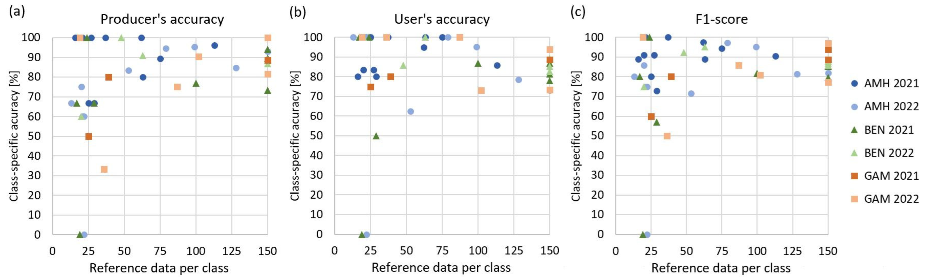
3.3.2. Crop Type Classification Accuracy Assessment

The crop type classification results retrieved with the best performing input dataset (Section 3.2) were validated using 20% of the available reference data, which were not used for training of the classifier. The validation results are provided in Figure S2. Additionally, class-specific F1-scores were derived, which are shown in Figure 8.
The classification for the Amhara study area for the year 2021 shows a high overall accuracy of 92% (Figure S2). Only a few class confusions occur. Systematic misclassifications cannot be observed. Several classes reach maximum possible producers’ or users’ accuracies (Figure S2). Figure 8 displays the class-specific F1-scores for individual study areas and years. For Amhara in 2021, maximum accuracies (100%) can be observed for haricot bean and finger millet. Sunflower (97%), soy bean (94%), maize, sesame, and mung bean (91%) also reach F1-scores greater than 90%, closely followed by wheat and teff (both 89%). Chickpea (80%) and pepper (73%) reach the lowest F1-scores for this classification.
The class-specific accuracies retrieved for Amhara 2022 are generally lower than for 2021, except for wheat and sunflower. The overall accuracy reaches 84% (Figure S2). It can be observed that most incorrect validation points have been assigned from other classes to maize (10 points from 122 total) and soy bean (6 points). The validation points for the pepper class could not be correctly classified for the year 2022 and were assigned to other classes (maize, soy, and mung bean) resulting in an F1-score of 0 (Figure 8). Sunflower (97%) and wheat (95%) reach high F1-scores, followed by haricot bean (86%), maize (82%), soy bean (81%), and finger millet (80%). F1-scores between 80% and 70% can be observed for sesame, teff (both 75%), and mung bean (71%).
The classification for Benishangul for 2021 includes eight classes. The overall accuracy is 82% (Figure S2). Except for niger seed and sesame, all classes reach F1-scores of 80% or higher (Figure 8). The highest F1-scores are achieved for teff (100%), maize, and sorghum (both 85%). The few validation points for sesame were not correctly classified and one point from niger seed was misclassified as sesame. Most classification errors, however, occurred because validation points were falsely classified as maize (9 points from 155 total) or sorghum (8 points), which, therefore, have reduced users’ accuracies (78% and 81% respectively). Some validation points from soy bean (12 points from 45, PA: 73%) and pepper (6 points from 26, PA: 77%) were assigned to other classes. Repeated class confusions can be observed between sorghum and soy bean (6 validation points) and soy bean and pepper (5 points, Figure S2).
The overall classification accuracy for Benishangul for the year 2022 is 88% (Figure S2). The highest F1-scores (Figure 8) are obtained for soy bean (95%) and niger seed (92%), followed by pepper (88%), maize (87%), sorghum (86%), and teff (75%). The F1-score for teff results from a low PA (60%) because only three of five validation points were classified correctly, while the UA is 100% (Figure S2).
For the classification for Gambela 2021, we obtain an overall accuracy of 89% (Figure S2). High F1-scores are obtained for mung bean (94%), cotton (89%), and maize (80%), while the F1-score for sorghum (60%) is lower (Figure 8), mainly because three of six validation points have been assigned to other classes (Figure S2).
The classification for Gambela for the year 2022 shows an overall accuracy of 85% (Figure S2). High F1-scores are observed for sesame (100%) and cotton (97%), followed by soy bean (86%), maize (81%), and mung bean (77%), as can be seen in Figure 8. Sorghum has again a low F1-score of only 50% and a low producer’s accuracy, because several validation points were not recognized correctly (Figure S2). Misclassifications generally occurred most often from other classes to mung bean (8 points) and maize (7 points) for Gambela 2022.
Regarding the validation results for individual crop type classes, it can be observed that false classifications often occur when validation points from rare classes are assigned to classes for which more reference data are available. Lower accuracies are generally observed for classes with fewer reference data, such as sesame, groundnut, and niger seed for Benishangul 2021, and teff for Benishangul 2022. For Gambela 2021, PA and UA are lowest for sorghum, which had the fewest reference data available (Table 5). The F1-scores obtained for sorghum in Gambela are relatively low for both years (50% and 60%), mainly due to low producers’ accuracies (Figure S2).
To further analyze and confirm this observation, we calculated diagrams showing the number of reference data per class and the class-specific producers’ and users’ accuracies, as well as F1-scores (Figure 9). We found that PAs are especially low for classes with few reference data (Figure 9). In general, accuracies below 70% only occur for classes with few reference data. Except for one single UA value (mung bean, Amhara 2022), all classes from all classifications with more than 40 reference data obtained accuracy values higher than 70% for PA, UA, and F1-Scores. Classes for which many reference data were available often have lower users’ accuracies compared to producers’ accuracies. This is caused by points from other classes being assigned to these classes (false positives).

4. Discussion

4.1. Classification Approach and Input Feature Importance

Within this study, we first classified LULC separately for both years of investigation and, in a second step, classified crop types for the identified cropland areas. This procedure was applied as there were no reliable annual cropland maps available for the study regions. Annual maps were required, as the study aimed at identifying land actually used as cropland for each specific year. Moreover, with the LULC classification, perennial tree crops, such as coffee and mango tree, could be separated. These classes do not compare to other crop types, which show a typical annual phenology, but have similar spectral and temporal characteristics compared to forest or shrubland. Therefore, the tree crop classes were already identified in the first step of the LULC classification.
In the context of this study, the LULC classification had the purpose of identifying the cropland areas to be included for subsequent crop type classification. For future studies with a focus on separating LULC classes, it may be useful to consider an a priori selection of classes based on, e.g., the taxonomy or spectral features. A hierarchical classification based on the FAO Land Cover Classification System (LCCS) taxonomy [107] might also be applied. A hierarchical classification would allow to aggregate classes and progressively increase the level of detail of the classes [108,109,110,111].
The comparison of different input datasets for crop type classification showed a high importance of Sentinel-2 spectral bands. The addition of Sentinel-1 parameters only slightly improved the accuracy compared to Sentinel-2 parameters alone. However, it reached the same or better accuracies for all six classification scenarios. In other studies, where a large number of different crop types were distinguished, a combination of several Sentinel-2 bands and Sentinel-1 parameters also proved to be advantageous. Asam et al. [18], for example, found that the best results for crop type classification were obtained by combining Sentinel-1 and Sentinel-2 data as input to a random forest classification for Germany. Sentinel-2 data alone also retrieved high F1-scores, while accuracies based on Sentinel-1 alone were lower for many crop types [18]. In another study on crop type classification in Germany, however, Sentinel-1 data were more important, but the best results were also obtained using a combination of Sentinel-1 and Sentinel-2 data [16]. In one study on the classification of soy bean and corn in the United States, the authors found that optical data were preferred over SAR by supervised algorithms such as decision trees [24]. For a study in Kenya, a more similar environment compared to our study, Aduvukha et al. [59] compared the performance of different input datasets for crop type classification and found that the best performing input dataset included variables of Sentinel-2, VIs, and Sentinel-1. Another study on crop mapping in West Africa also reported that the integration of both optical (RapidEye) and SAR (TerraSAR-X) data improved the classification accuracy [61].

4.2. Classification Results and Influence of Reference Data on Accuracies Obtained

For LULC and crop type classification, mostly supervised classification methods are applied. Therefore, accurate reference data are of great importance for reliable classification results, especially for crop type classification, where field data are usually required [112]. Regarding the cropland classification of our study, the LULC classifier relied on sample data collected based on remote sensing imagery, as the field data collection concentrated on in situ data for crop types. In the case of the natural vegetation classes, the separation between similar classes was often difficult. This was no obstacle for the purpose of this study, as the focus was on outlining cropland areas. Therefore, the separation between other classes was of less importance. The collection of separate samples for the classes tree cover and shrubland, as well as shrubland, grassland, and sparse vegetation was especially difficult due to a gradual transition between these classes. Difficulties in separating natural vegetation classes were also observed, e.g., by Eggen et al. [45], who classified LULC in the Ethiopian highlands and found that the observed confusion among grassland, woodland, and barren categories reflects the difficulty of classifying savannah landscapes, especially in eastern Central Africa. Moreover, they state that the monsoonal-driven rainfall patterns leading to cloud coverage for significant periods of time make class separation more difficult.
The supervised crop type classification of this study was trained using field data collected for the three study areas in the years 2021 and 2022 (Section 2.2.4). The in situ data were collected for a broad range of crop types. In total, field data for 18 different crop types were available for the classification. This is a very valuable database for crop type classification. The spatial distribution of field data over the Amhara study area was good for both years. For the western part of the Benishangul study area, no field data were collected in 2021, as this area was not accessible during the field campaign due to security reasons. For Gambela, field data were available from different parts of the study area, though for 2022, no data were available from the most northern part. The distribution of field data among crop types was not optimal from the perspective of remote sensing classification. For some crop types, only a few field data were collected, while for others, large sample sizes were available. Having a look at the class-specific accuracies, we found that for classes with few reference data especially, PAs were low (Figure 9). Classes with more than 40 reference data mostly obtained accuracy values higher than 70% for PA, UA, and F1-Scores. Based on these observations, we suggest collecting at least 40 to 50 points for the not-so-frequent crop type classes as well for future data collections in these or similar study regions. This can be expected to improve the class-specific accuracies, especially for the rare classes, but also the UA of the more frequent classes.
For future field surveys in the study areas, the cropland and crop type maps derived in this study can be used to provide a priori information about expected class sizes and locations. This could assist in optimizing survey routes or selecting target areas for setting up, for example, clustering schemes or sequential exploration methods to identify the most important fields to survey [112,113].

4.3. Outlook

The monitoring of different types of agricultural areas might become increasingly important for Sub-Saharan Africa due to climate change affecting agricultural productivity, especially for smallholder farms [114,115]. Due to the relatively high spatial resolution (10 m) of the classification results of this study, the classification approach used can also be applied for monitoring smallholder farms in Ethiopia and comparable regions and, thus, contribute to developing sustainable agricultural management in these regions.
The classification algorithm is designed to be applicable for monitoring cropland and crop types in the study areas for future years as well. As this is a supervised classification, reference data have to be available for the study area and year of interest.
Future research could be dedicated to testing how the random forest classifier that was trained for one study area and year performs in classifying another area or year. Random forest classifiers potentially allow for transferability [25]. In one study by Wang et al. [31], a random forest transfer was tested and the authors found that transfer to neighboring geographies is possible when regional crop compositions and growing conditions are similar [31].
The final classification results from this study derived the actual land used for agriculture and crop types grown in the three study areas. Unproductive lands become visible and land managers can take measures to improve land use efficiency accordingly. Therefore, remote sensing offers the potential to improve and support the performance monitoring of agricultural investments in Ethiopia. The information products on cropland and crop types can potentially also be integrated in agricultural management information systems and form the basis for further analyses on topics such as crop yield estimation and agricultural revenue generation.

5. Conclusions

The aim of this study was to develop a remote sensing method for mapping cropland and crop types for large-scale agricultural investment (LSAI) areas in Ethiopia. The method development was based on open-source Sentinel-1 and Sentinel-2 time series and implemented in Google Earth Engine (GEE) to allow for the application by regional experts without their own remote sensing classification software and large computational infrastructure.
In order to select a robust input dataset, 198 different crop type classifications based on 33 variants of input data for three study areas and two years of investigation were calculated. The comparison of input datasets for crop type classification produced the following findings: (1) The individual VIs retrieved similar overall accuracies of on average 75%, but showed large differences in accuracies for individual classifications ranging from 59% to 89%. (2) The combination of two or three VIs improves the average accuracy to about 81% and reduced the variation of individual classifications. (3) Accuracies obtained based on Sentinel-1 parameters alone were comparatively low and reached about 71% overall accuracy. The combination of VV, VH, and Diff obtained the highest accuracies within the variants of Sentinel-1 input datasets. (4) The seven best performing input datasets all made use of Sentinel-2 bands and retrieved average accuracies >84%. (5) The addition of Sentinel-1 parameters only slightly improved the accuracy compared to using Sentinel-2 parameters alone. (6) From the variants tested in this study, the best performing input dataset with the most robust results included the following parameters: S2 bands, EVI2 and NDRe2 from Sentinel-2, and VV, VH, and Diff from Sentinel-1.
The accuracy assessment of the LULC classification showed F1-scores for cropland ranging between 89% and 95%. The crop type classifications for the six classification scenarios retrieved overall accuracies between 82% and 92%. Comparing the number of reference data per class and the class-specific accuracies obtained, we found that low accuracies (<70%) for PA, UA, or F1-score only occurred for classes with few (<40) reference data.
With respect to the classification results for the three study areas, our findings were as follows: (1) In Amhara study area, about 80% of LSAI areas were used for growing crops. The most common crop was maize, followed by soy bean and wheat. (2) In Benishangul, about 20% of LSAI areas were used as cropland. The most important crops were maize and sorghum. (3) In the Gambela study area, 17% and 21% of the LSAI areas were used for crop production in 2021 and 2022, respectively, with the most important crops being mung bean and cotton. These results indicate a great potential for further cropland development, especially in the Benishangul and Gambela study areas.
In this study, we classified cropland and crop types for three study areas in Ethiopia. We separated a comparatively large number of 18 different crop types. For the study areas in Ethiopia, such detailed crop type classification and corresponding information products on spatial distribution of land used for agricultural production and crop types grown have not been available before. The classification approach was implemented in a cloud-processing environment in order to enable uptake by regional experts and decision-makers from resource-constrained institutions without their own large computational software and capacities. The developed classification method is designed to allow application in further years and to similar study areas.

Supplementary Materials

The following supporting information can be downloaded at: https://www.mdpi.com/article/10.3390/rs16050866/s1, Figure S1: Confusion matrix tables for the LULC classifications for the three study areas Amhara, Benishangul, and Gambela for the years 2021 and 2022. The accuracies are given as users’ accuracies (UAs), producers’ accuracies (PAs) and overall accuracy (OA); Figure S2: Confusion matrix tables for the crop type classifications for the three study areas Amhara, Benishangul, and Gambela for the years 2021 and 2022. The accuracies are given as users’ accuracies (UAs), producers’ accuracies (PAs) and overall accuracy (OA); Table S1: Overview of the 33 input data variants tested for random forest crop type classification. The table provides information about variant category (column 1), bands/indices/parameters included (column 2), number of input bands (column 3), and overall accuracies retrieved (columns 4–12). The overall accuracies are provided for the six individual classifications, as average for each study area, and as an overall mean.

Author Contributions

Conceptualization, C.E.; methodology, C.E.; software, C.E. and B.B.; validation, C.E.; formal analysis, C.E., B.B. and P.S.; investigation, C.E.; resources, C.E., R.H., G.A. and C.M.; writing—original draft preparation, C.E.; writing—review and editing, C.E., U.G., B.B., P.S. and J.H.; visualization, C.E.; project administration, C.E. and C.M.; funding acquisition, C.E., J.H. and C.M. All authors have read and agreed to the published version of the manuscript.

Funding

This research was carried out at the German Aerospace Center (DLR) as part of the Ethiopian country packages “Support to Responsible Agricultural Investment” (S2RAI) and “Promoting Responsible Governance of Investments in Land” (RGIL) of the global program on Responsible Land Policy implemented by the Deutsche Gesellschaft für Internationale Zusammenarbeit (GIZ) GmbH on behalf of the Federal Government of Germany. The project is co-funded by the European Union [DCI/FOOD/2019/408-937] and the German Federal Ministry for Economic Cooperation and Development (BMZ) [15.0124.6-008.00].

Data Availability Statement

The data presented in this study are available on request from the corresponding author. The data are not publicly available due to ongoing research.

Acknowledgments

We acknowledge both the German Federal Ministry for Economic Cooperation and Development (BMZ) and the Deutsche Gesellschaft für Internationale Zusammenarbeit (GIZ) GmbH for their financial and technical support, respectively. We further thank GIZ for providing in situ data for this project. We thank the four anonymous reviewers for their constructive comments that helped to improve this article.

Conflicts of Interest

Authors Genanaw Alemu, Rahel Hailu and Christian Mesmer were employed by the company Deutsche Gesellschaft für Internationale Zusammenarbeit (GIZ) GmbH. The remaining authors declare that the research was conducted in the absence of any commercial or financial relationships that could be construed as a potential conflict of interest.

References

  1. FAOSTAT. Data. Available online: https://www.fao.org/faostat/en/#data (accessed on 27 October 2023).
  2. UNFCCC. Ethiopia. A Case Study Conducted by the Climate Resilient Food Systems Alliance. 2022. Available online: https://unfccc.int/sites/default/files/resource/Ethiopia_CRFS_Case_Study.pdf (accessed on 26 October 2023).
  3. GIZ. Ensuring Food Security and Land Tenure. Available online: https://www.giz.de/en/worldwide/83147.html (accessed on 21 September 2023).
  4. Guo, Z. Map Teff in Ethiopia: An Approach to Integrate Time Series Remotely Sensed Data and Household Data at Large Scale. In Proceedings of the IEEE Joint International Geoscience and Remote Sensing Symposium (IGARSS)/35th Canadian Symposium on Remote Sensing, Quebec City, QC, Canada, 13–18 July 2014; pp. 2138–2141. [Google Scholar]
  5. Cheng, G.; Ding, H.; Yang, J.; Cheng, Y.S. Crop type classification with combined spectral, texture, and radar features of time-series Sentinel-1 and Sentinel-2 data. Int. J. Remote Sens. 2023, 44, 1215–1237. [Google Scholar] [CrossRef]
  6. Belgiu, M.; Csillik, O. Sentinel-2 cropland mapping using pixel-based and object-based time-weighted dynamic time warping analysis. Remote Sens. Environ. 2018, 204, 509–523. [Google Scholar] [CrossRef]
  7. Ouzemou, J.-E.; El Harti, A.; Lhissou, R.; El Moujahid, A.; Bouch, N.; El Ouazzani, R.; Bachaoui, E.M.; El Ghmari, A. Crop type mapping from pansharpened Landsat 8 NDVI data: A case of a highly fragmented and intensive agricultural system. Remote Sens. Appl. Soc. Environ. 2018, 11, 94–103. [Google Scholar] [CrossRef]
  8. Kobayashi, N.; Tani, H.; Wang, X.; Sonobe, R. Crop classification using spectral indices derived from Sentinel-2A imagery. J. Inf. Telecommun. 2020, 4, 67–90. [Google Scholar] [CrossRef]
  9. Dong, T.; Liu, J.; Shang, J.; Qian, B.; Ma, B.; Kovacs, J.M.; Walters, D.; Jiao, X.; Geng, X.; Shi, Y. Assessment of red-edge vegetation indices for crop leaf area index estimation. Remote Sens. Environ. 2019, 222, 133–143. [Google Scholar] [CrossRef]
  10. Zeng, Y.L.; Hao, D.L.; Huete, A.; Dechant, B.; Berry, J.; Chen, J.M.; Joiner, J.; Frankenberg, C.; Bond-Lamberty, B.; Ryu, Y.; et al. Optical vegetation indices for monitoring terrestrial ecosystems globally. Nat. Rev. Earth Env. 2022, 3, 477–493. [Google Scholar] [CrossRef]
  11. Schlund, M.; Erasmi, S. Sentinel-1 time series data for monitoring the phenology of winter wheat. Remote Sens. Environ. 2020, 246, 111814. [Google Scholar] [CrossRef]
  12. Selvaraj, S.; Haldar, D.; Srivastava, H.S. Condition assessment of pearl millet/ bajra crop in different vigour zones using Radar Vegetation Index. Spat. Inf. Res. 2021, 29, 631–643. [Google Scholar] [CrossRef]
  13. Mercier, A.; Betbeder, J.; Denize, J.; Roger, J.-L.; Spicher, F.; Lacoux, J.; Roger, D.; Baudry, J.; Hubert-Moy, L. Estimating crop parameters using Sentinel-1 and 2 datasets and geospatial field data. Data Brief 2021, 38, 107408. [Google Scholar] [CrossRef] [PubMed]
  14. Meroni, M.; d’Andrimont, R.; Vrieling, A.; Fasbender, D.; Lemoine, G.; Rembold, F.; Seguini, L.; Verhegghen, A. Comparing land surface phenology of major European crops as derived from SAR and multispectral data of Sentinel-1 and-2. Remote Sens. Environ. 2021, 253, 112232. [Google Scholar] [CrossRef]
  15. Salehi, B.; Daneshfar, B.; Davidson, A.M. Accurate crop-type classification using multi-temporal optical and multi-polarization SAR data in an object-based image analysis framework. Int. J. Remote Sens. 2017, 38, 4130–4155. [Google Scholar] [CrossRef]
  16. Orynbaikyzy, A.; Gessner, U.; Mack, B.; Conrad, C. Crop Type Classification Using Fusion of Sentinel-1 and Sentinel-2 Data: Assessing the Impact of Feature Selection, Optical Data Availability, and Parcel Sizes on the Accuracies. Remote Sens. 2020, 12, 2779. [Google Scholar] [CrossRef]
  17. Chakhar, A.; Hernandez-Lopez, D.; Ballesteros, R.; Moreno, M.A. Improving the Accuracy of Multiple Algorithms for Crop Classification by Integrating Sentinel-1 Observations with Sentinel-2 Data. Remote Sens. 2021, 13, 243. [Google Scholar] [CrossRef]
  18. Asam, S.; Gessner, U.; Gonzalez, R.A.; Wenzl, M.; Kriese, J.; Kuenzer, C. Mapping Crop Types of Germany by Combining Temporal Statistical Metrics of Sentinel-1 and Sentinel-2 Time Series with LPIS Data. Remote Sens. 2022, 14, 2981. [Google Scholar] [CrossRef]
  19. Blickensdörfer, L.; Schwieder, M.; Pflugmacher, D.; Nendel, C.; Erasmi, S.; Hostert, P. Mapping of crop types and crop sequences with combined time series of Sentinel-1, Sentinel-2 and Landsat 8 data for Germany. Remote Sens. Environ. 2022, 269, 112831. [Google Scholar] [CrossRef]
  20. Katal, N.; Hooda, N.; Sharma, A.; Sharma, B. Cropland prediction using remote sensing, ancillary data, and machine learning. J. Appl. Remote Sens. 2022, 17, 022202. [Google Scholar] [CrossRef]
  21. Orynbaikyzy, A.; Gessner, U.; Conrad, C. Crop type classification using a combination of optical and radar remote sensing data: A review. Int. J. Remote Sens. 2019, 40, 6553–6595. [Google Scholar] [CrossRef]
  22. d’Andrimont, R.; Verhegghen, A.; Lemoine, G.; Kempeneers, P.; Meroni, M.; van der Velde, M. From parcel to continental scale—A first European crop type map based on Sentinel-1 and LUCAS Copernicus in-situ observations. Remote Sens. Environ. 2021, 266, 112708. [Google Scholar] [CrossRef]
  23. Luo, C.; Liu, H.; Lu, L.; Liu, Z.; Kong, F.; Zhang, X. Monthly composites from Sentinel-1 and Sentinel-2 images for regional major crop mapping with Google Earth Engine. J. Integr. Agric. 2021, 20, 1944–1957. [Google Scholar] [CrossRef]
  24. Song, X.-P.; Huang, W.; Hansen, M.C.; Potapov, P. An evaluation of Landsat, Sentinel-2, Sentinel-1 and MODIS data for crop type mapping. Sci. Remote Sens. 2021, 3, 100018. [Google Scholar] [CrossRef]
  25. Orynbaikyzy, A.; Gessner, U.; Conrad, C. Spatial Transferability of Random Forest Models for Crop Type Classification Using Sentinel-1 and Sentinel-2. Remote Sens. 2022, 14, 1493. [Google Scholar] [CrossRef]
  26. Rivera, A.J.; Pérez-Godoy, M.D.; Elizondo, D.; Deka, L.; del Jesus, M.J. Analysis of clustering methods for crop type mapping using satellite imagery. Neurocomputing 2022, 492, 91–106. [Google Scholar] [CrossRef]
  27. Solano-Correa, Y.T.; Bovolo, F.; Bruzzone, L. A Semi-Supervised Crop-Type Classification Based on Sentinel-2 NDVI Satellite Image Time Series and Phenological Parameters. In Proceedings of the IGARSS 2019–2019 IEEE International Geoscience and Remote Sensing Symposium, Yokohama, Japan, 28 July–2 August 2019; pp. 457–460. [Google Scholar]
  28. Lin, C.; Zhong, L.; Song, X.-P.; Dong, J.; Lobell, D.B.; Jin, Z. Early- and in-season crop type mapping without current-year ground truth: Generating labels from historical information via a topology-based approach. Remote Sens. Environ. 2022, 274, 112994. [Google Scholar] [CrossRef]
  29. Johnson, D.M.; Mueller, R. Pre- and within-season crop type classification trained with archival land cover information. Remote Sens. Environ. 2021, 264, 112576. [Google Scholar] [CrossRef]
  30. Rußwurm, M.; Courty, N.; Emonet, R.; Lefèvre, S.; Tuia, D.; Tavenard, R. End-to-end learned early classification of time series for in-season crop type mapping. ISPRS J. Photogramm. Remote Sens. 2023, 196, 445–456. [Google Scholar] [CrossRef]
  31. Wang, S.; Azzari, G.; Lobell, D.B. Crop type mapping without field-level labels: Random forest transfer and unsupervised clustering techniques. Remote Sens. Environ. 2019, 222, 303–317. [Google Scholar] [CrossRef]
  32. Jin, Z.; Azzari, G.; You, C.; Di Tommaso, S.; Aston, S.; Burke, M.; Lobell, D.B. Smallholder maize area and yield mapping at national scales with Google Earth Engine. Remote Sens. Environ. 2019, 228, 115–128. [Google Scholar] [CrossRef]
  33. Gorelick, N.; Hancher, M.; Dixon, M.; Ilyushchenko, S.; Thau, D.; Moore, R. Google Earth Engine: Planetary-scale geospatial analysis for everyone. Remote Sens. Environ. 2017, 202, 18–27. [Google Scholar] [CrossRef]
  34. Ali, H.; Descheemaeker, K.; Steenhuis, T.S.; Pandey, S. Comparison of landuse and landcover changes, drivers and impacts for a moisture-sufficient and drought-prone region in the Ethiopian highlands. Exp. Agric. 2011, 47, 71–83. [Google Scholar] [CrossRef]
  35. Daba, M.H.; You, S.C. Quantitatively Assessing the Future Land-Use/Land-Cover Changes and Their Driving Factors in the Upper Stream of the Awash River Based on the CA-Markov Model and Their Implications for Water Resources Management. Sustainability 2022, 14, 1538. [Google Scholar] [CrossRef]
  36. Dega, M.B.; Emana, A.N.; Feda, H.A. The Impact of Catchment Land Use Land Cover Changes on Lake Dandi, Ethiopia. J. Environ. Public Health 2022, 2022, 4936289. [Google Scholar] [CrossRef] [PubMed]
  37. Desalegn, T.; Cruz, F.; Kindu, M.; Turrion, M.B.; Gonzalo, J. Land-use/land-cover (LULC) change and socioeconomic conditions of local community in the central highlands of Ethiopia. Int. J. Sustain. Dev. World Ecol. 2014, 21, 406–413. [Google Scholar] [CrossRef]
  38. Desta, Y.; Goitom, H.; Aregay, G. Investigation of runoff response to land use/land cover change on the case of Aynalem catchment, North of Ethiopia. J. Afr. Earth Sci. 2019, 153, 130–143. [Google Scholar] [CrossRef]
  39. Mariye, M.; Li, J.H.; Maryo, M. Land use and land cover change, and analysis of its drivers in Ojoje watershed, Southern Ethiopia. Heliyon 2022, 8, e09267. [Google Scholar] [CrossRef]
  40. Mekasha, S.T.; Suryabhagavan, K.V.; Gebrehiwot, M. Geo-spatial approach for land-use and land-cover changes and deforestation mapping: A case study of Ankasha Guagusa, Northwestern, Ethiopia. Trop. Ecol. 2020, 61, 550–569. [Google Scholar] [CrossRef]
  41. Minta, M.; Kibret, K.; Thorne, P.; Nigussie, T.; Nigatu, L. Land use and land cover dynamics in Dendi-Jeldu hilly-mountainous areas in the central Ethiopian highlands. Geoderma 2018, 314, 27–36. [Google Scholar] [CrossRef]
  42. Moges, D.M.; Bhat, H.G. An insight into land use and land cover changes and their impacts in Rib watershed, north-western highland Ethiopia. Land Degrad. Dev. 2018, 29, 3317–3330. [Google Scholar] [CrossRef]
  43. Wondrade, N.; Dick, O.B.; Tveite, H. GIS based mapping of land cover changes utilizing multi-temporal remotely sensed image data in Lake Hawassa Watershed, Ethiopia. Environ. Monit. Assess. 2014, 186, 1765–1780. [Google Scholar] [CrossRef]
  44. Yeshaneh, E.; Wagner, W.; Exner-Kittridge, M.; Legesse, D.; Bloschl, G. Identifying Land Use/Cover Dynamics in the Koga Catchment, Ethiopia, from Multi-Scale Data, and Implications for Environmental Change. ISPRS Int. J. Geo-Inf. 2013, 2, 302–323. [Google Scholar] [CrossRef]
  45. Eggen, M.; Ozdogan, M.; Zaitchik, B.F.; Simane, B. Land Cover Classification in Complex and Fragmented Agricultural Landscapes of the Ethiopian Highlands. Remote Sens. 2016, 8, 1020. [Google Scholar] [CrossRef]
  46. Xu, Y.D.; Yu, L.; Peng, D.L.; Cai, X.L.; Cheng, Y.Q.; Zhao, J.Y.; Zhao, Y.Y.; Feng, D.L.; Hackman, K.; Huang, X.M.; et al. Exploring the temporal density of Landsat observations for cropland mapping: Experiments from Egypt, Ethiopia, and South Africa. Int. J. Remote Sens. 2018, 39, 7328–7349. [Google Scholar] [CrossRef]
  47. Assefa, E.; Bork, H.R. Dynamics and driving forces of agricultural landscapes in Southern Ethiopia—A case study of the Chencha and Arbaminch areas. J. Land Use Sci. 2016, 11, 278–293. [Google Scholar] [CrossRef]
  48. Abera, A.; Verhoest, N.E.C.; Tilahun, S.; Inyang, H.; Nyssen, J. Assessment of irrigation expansion and implications for water resources by using RS and GIS techniques in the Lake Tana Basin of Ethiopia. Environ. Monit. Assess. 2021, 193, 13. [Google Scholar] [CrossRef]
  49. Gessesse, B.; Tesfamariam, B.G.; Melgani, F. Understanding traditional agro-ecosystem dynamics in response to systematic transition processes and rainfall variability patterns at watershed-scale in Southern Ethiopia. Agric. Ecosyst. Environ. 2022, 327, 107832. [Google Scholar] [CrossRef]
  50. Husak, G.J.; Marshall, M.T.; Michaelsen, J.; Pedreros, D.; Funk, C.; Galu, G. Crop area estimation using high and medium resolution satellite imagery in areas with complex topography. J. Geophys. Res. Atmos. 2008, 113, D14112. [Google Scholar] [CrossRef]
  51. McCarty, J.L.; Neigh, C.S.R.; Carroll, M.L.; Wooten, M.R. Extracting smallholder cropped area in Tigray, Ethiopia with wall-to-wall sub-meter WorldView and moderate resolution Landsat 8 imagery. Remote Sens. Environ. 2017, 202, 142–151. [Google Scholar] [CrossRef]
  52. Mohammed, I.; Marshall, M.; de Bie, K.; Estes, L.; Nelson, A. A blended census and multiscale remote sensing approach to probabilistic cropland mapping in complex landscapes. ISPRS J. Photogramm. Remote Sens. 2020, 161, 233–245. [Google Scholar] [CrossRef]
  53. Neigh, C.S.R.; Carroll, M.L.; Wooten, M.R.; McCarty, J.L.; Powell, B.F.; Husak, G.J.; Enenkel, M.; Hain, C.R. Smallholder crop area mapped with wall-to-wall WorldView sub-meter panchromatic image texture: A test case for Tigray, Ethiopia. Remote Sens. Environ. 2018, 212, 8–20. [Google Scholar] [CrossRef]
  54. Vogels, M.F.A.; de Jong, S.M.; Sterk, G.; Addink, E.A. Agricultural cropland mapping using black-and-white aerial photography, Object-Based Image Analysis and Random Forests. Int. J. Appl. Earth Obs. Geoinf. 2017, 54, 114–123. [Google Scholar] [CrossRef]
  55. Sahle, M.; Yeshitela, K.; Saito, O. Mapping the supply and demand of Enset crop to improve food security in Southern Ethiopia. Agron. Sustain. Dev. 2018, 38, 7. [Google Scholar] [CrossRef]
  56. Gilbertson, J.K.; Kemp, J.; van Niekerk, A. Effect of pan-sharpening multi-temporal Landsat 8 imagery for crop type differentiation using different classification techniques. Comput. Electron. Agric. 2017, 134, 151–159. [Google Scholar] [CrossRef]
  57. Maponya, M.G.; van Niekerk, A.; Mashimbye, Z.E. Pre-harvest classification of crop types using a Sentinel-2 time-series and machine learning. Comput. Electron. Agric. 2020, 169, 105164. [Google Scholar] [CrossRef]
  58. Aduvukha, G.R.; Abdel-Rahman, E.M.; Sichangi, A.W.; Makokha, G.O.; Landmann, T.; Mudereri, B.T.; Tonnang, H.E.Z.; Dubois, T. Cropping Pattern Mapping in an Agro-Natural Heterogeneous Landscape Using Sentinel-2 and Sentinel-1 Satellite Datasets. Agriculture 2021, 11, 530. [Google Scholar] [CrossRef]
  59. Kerner, H.; Nakalembe, C.; Becker-Reshef, I. Field-Level Crop Type Classification with k Nearest Neighbors: A Baseline for a New Kenya Smallholder Dataset. In Proceedings of the ICLR 2020 Workshop on Computer Vision for Agriculture, Addis Ababa, Ethiopia, 26 April 2020. [Google Scholar]
  60. Forkuor, G.; Conrad, C.; Thiel, M.; Ullmann, T.; Zoungrana, E. Integration of Optical and Synthetic Aperture Radar Imagery for Improving Crop Mapping in Northwestern Benin, West Africa. Remote Sens. 2014, 6, 6472–6499. [Google Scholar] [CrossRef]
  61. Elders, A.; Carroll, M.L.; Neigh, C.S.R.; D’Agostino, A.L.; Ksoll, C.; Wooten, M.R.; Brown, M.E. Estimating crop type and yield of small holder fields in Burkina Faso using multi-day Sentinel-2. Remote Sens. Appl. Soc. Environ. 2022, 27, 100820. [Google Scholar] [CrossRef]
  62. Forkuor, G.; Conrad, C.; Thiel, M.; Landmann, T.; Barry, B. Evaluating the sequential masking classification approach for improving crop discrimination in the Sudanian Savanna of West Africa. Comput. Electron. Agric. 2015, 118, 380–389. [Google Scholar] [CrossRef]
  63. Aguilar, R.; Zurita-Milla, R.; Izquierdo-Verdiguier, E.; de By, R.A. A Cloud-Based Multi-Temporal Ensemble Classifier to Map Smallholder Farming Systems. Remote Sens. 2018, 10, 729. [Google Scholar] [CrossRef]
  64. Lambert, M.-J.; Traoré, P.C.S.; Blaes, X.; Baret, P.; Defourny, P. Estimating smallholder crops production at village level from Sentinel-2 time series in Mali’s cotton belt. Remote Sens. Environ. 2018, 216, 647–657. [Google Scholar] [CrossRef]
  65. Lebourgeois, V.; Dupuy, S.; Vintrou, É.; Ameline, M.; Butler, S.; Bégué, A. A Combined Random Forest and OBIA Classification Scheme for Mapping Smallholder Agriculture at Different Nomenclature Levels Using Multisource Data (Simulated Sentinel-2 Time Series, VHRS and DEM). Remote Sens. 2017, 9, 259. [Google Scholar] [CrossRef]
  66. Becker-Reshef, I.; Barker, B.; Whitcraft, A.; Oliva, P.; Mobley, K.; Justice, C.; Sahajpal, R. Crop Type Maps for Operational Global Agricultural Monitoring. Sci. Data 2023, 10, 172. [Google Scholar] [CrossRef]
  67. NASA. Shuttle Radar Topograpy Mission (SRTM). Available online: https://www.earthdata.nasa.gov/sensors/srtm (accessed on 20 March 2023).
  68. Zepner, L.; Karrasch, P.; Wiemann, F.; Bernard, L. ClimateCharts.net—An interactive climate analysis web platform. Int. J. Digit. Earth 2021, 14, 338–356. [Google Scholar] [CrossRef]
  69. FAO; IIASA. Global Agro Ecological Zones Version 4 (GAEZ v4). Available online: http://www.fao.org/gaez/ (accessed on 22 March 2023).
  70. FAO. Crop Calendar. Available online: https://cropcalendar.apps.fao.org/ (accessed on 20 March 2023).
  71. ESA. Sentinel-2 User Handbook. Available online: https://sentinel.esa.int/documents/247904/685211/Sentinel-2_User_Handbook (accessed on 25 September 2023).
  72. Google_Developers. Earth Engine Data Catalog. Harmonized Sentinel-2 MSI: MultiSpectral Instrument, Level-2A. Available online: https://developers.google.com/earth-engine/datasets/catalog/COPERNICUS_S2_SR_HARMONIZED (accessed on 25 September 2023).
  73. Google_Developers. Earth Engine Data Catalog. Sentinel-2: Cloud Probability. Available online: https://developers.google.com/earth-engine/datasets/catalog/COPERNICUS_S2_CLOUD_PROBABILITY (accessed on 25 September 2023).
  74. Kamenova, I.; Dimitrov, P. Evaluation of Sentinel-2 vegetation indices for prediction of LAI, fAPAR and fCover of winter wheat in Bulgaria. Eur. J. Remote Sens. 2021, 54, 89–108. [Google Scholar] [CrossRef]
  75. Chen, D.Y.; Huang, J.F.; Jackson, T.J. Vegetation water content estimation for corn and soybeans using spectral indices derived from MODIS near- and short-wave infrared bands. Remote Sens. Environ. 2005, 98, 225–236. [Google Scholar] [CrossRef]
  76. Xie, G.Y.; Niculescu, S. Mapping Crop Types Using Sentinel-2 Data Machine Learning and Monitoring Crop Phenology with Sentinel-1 Backscatter Time Series in Pays de Brest, Brittany, France. Remote Sens. 2022, 14, 4437. [Google Scholar] [CrossRef]
  77. Holtgrave, A.K.; Röder, N.; Ackermann, A.; Erasmi, S.; Kleinschmit, B. Comparing Sentinel-1 and-2 Data and Indices for Agricultural Land Use Monitoring. Remote Sens. 2020, 12, 2919. [Google Scholar] [CrossRef]
  78. Palchowdhuri, Y.; Valcarce-Diñeiro, R.; King, P.; Sanabria-Soto, M. Classification of multi-temporal spectral indices for crop type mapping: A case study in Coalville, UK. J. Agric. Sci. 2018, 156, 24–36. [Google Scholar] [CrossRef]
  79. Rouse, J.W.; Haas, R.H.; Schell, J.A.; Deering, D.W. Monitoring vegetation systems in the great plains with ERTS. NASA Spec. Publ. 1974, 351, 309. [Google Scholar]
  80. Chen, J.M. Evaluation of Vegetation Indices and a Modified Simple Ratio for Boreal Applications. Can. J. Remote Sens. 1996, 22, 229–242. [Google Scholar] [CrossRef]
  81. Liu, H.Q.; Huete, A.R. A feedback based modification of the NDVI to minimize canopy background and atmospheric noise. IEEE Trans. Geosci. Remote Sens. 1995, 33, 457–465. [Google Scholar] [CrossRef]
  82. Huete, A.; Didan, K.; Miura, T.; Rodriguez, E.P.; Gao, X.; Ferreira, L.G. Overview of the radiometric and biophysical performance of the MODIS vegetation indices. Remote Sens. Environ. 2002, 83, 195–213. [Google Scholar] [CrossRef]
  83. Jiang, Z.Y.; Huete, A.R.; Didan, K.; Miura, T. Development of a two-band enhanced vegetation index without a blue band. Remote Sens. Environ. 2008, 112, 3833–3845. [Google Scholar] [CrossRef]
  84. Huete, A.R. A Soil-Adjusted Vegetation Index (Savi). Remote Sens. Environ. 1988, 25, 295–309. [Google Scholar] [CrossRef]
  85. Gitelson, A.A.; Kaufman, Y.J.; Merzlyak, M.N. Use of a green channel in remote sensing of global vegetation from EOS-MODIS. Remote Sens. Environ. 1996, 58, 289–298. [Google Scholar] [CrossRef]
  86. Gitelson, A.; Merzlyak, M.N. Spectral Reflectance Changes Associated with Autumn Senescence of Aesculus-Hippocastanum L and Acer-Platanoides L Leaves—Spectral Features and Relation to Chlorophyll Estimation. J. Plant Physiol. 1994, 143, 286–292. [Google Scholar] [CrossRef]
  87. Sims, D.A.; Gamon, J.A. Relationships between leaf pigment content and spectral reflectance across a wide range of species, leaf structures and developmental stages. Remote Sens. Environ. 2002, 81, 337–354. [Google Scholar] [CrossRef]
  88. Barnes, E.; Clarke, T.R.; Richards, S.E.; Colaizzi, P.; Haberland, J.; Kostrzewski, M.; Waller, P.; Choi, C.; Riley, E.; Thompson, T.L. Coincident detection of crop water stress, nitrogen status, and canopy density using ground based multispectral data. In Proceedings of the Fifth International Conference on Precision Agriculture, Bloomington, MN, USA, 16–19 July 2000. [Google Scholar]
  89. McFeeters, S.K. The use of the normalized difference water index (NDWI) in the delineation of open water features. Int. J. Remote Sens. 1996, 17, 1425–1432. [Google Scholar] [CrossRef]
  90. Ghosh, S.M.; Saraf, S.; Behera, M.D.; Biradar, C. Estimating Agricultural Crop Types and Fallow Lands Using Multi Temporal Sentinel-2A Imageries. Proc. Natl. Acad. Sci. USA 2017, 87, 769–779. [Google Scholar] [CrossRef]
  91. Gao, B.C. NDWI—A normalized difference water index for remote sensing of vegetation liquid water from space. Remote Sens. Environ. 1996, 58, 257–266. [Google Scholar] [CrossRef]
  92. ESA. Sentinel-1 SAR User Guide. Available online: https://sentinel.esa.int/web/sentinel/user-guides/sentinel-1-sar/ (accessed on 25 September 2023).
  93. Google_Developers. Earth Engine Data Catalog. Sentinel-1 SAR GRD: C-Band Synthetic Aperture Radar Ground Range Detected, Log Scaling. Available online: https://developers.google.com/earth-engine/datasets/catalog/COPERNICUS_S1_GRD (accessed on 27 September 2023).
  94. Mullissa, A.; Vollrath, A.; Odongo-Braun, C.; Slagter, B.; Balling, J.; Gou, Y.; Gorelick, N.; Reiche, J. Sentinel-1 SAR Backscatter Analysis Ready Data Preparation in Google Earth Engine. Remote Sens. 2021, 13, 1954. [Google Scholar] [CrossRef]
  95. ESA. Sentinel-1 Observation Scenario. Available online: https://sentinel.esa.int/web/sentinel/missions/sentinel-1/observation-scenario (accessed on 28 September 2023).
  96. Fu, B.L.; Xie, S.Y.; He, H.C.; Zuo, P.P.; Sun, J.; Liu, L.L.; Huang, L.K.; Fan, D.L.; Gao, E.R. Synergy of multi-temporal polarimetric SAR and optical image satellite for mapping of marsh vegetation using object-based random forest algorithm. Ecol. Indic. 2021, 131, 108173. [Google Scholar] [CrossRef]
  97. Lee, J.S.; Wen, J.H.; Ainsworth, T.L.; Chen, K.S.; Chen, A.J. Improved Sigma Filter for Speckle Filtering of SAR Imagery. IEEE Trans. Geosci. Remote Sens. 2009, 47, 202–213. [Google Scholar] [CrossRef]
  98. Dong, J.W.; Xiao, X.M.; Chen, B.Q.; Torbick, N.; Jin, C.; Zhang, G.L.; Biradar, C. Mapping deciduous rubber plantations through integration of PALSAR and multi-temporal Landsat imagery. Remote Sens. Environ. 2013, 134, 392–402. [Google Scholar] [CrossRef]
  99. JAXA. ALOS Global Digital Surface Model (DSM). ALOS World 3D-30m (AW3D30). Version 2.2. Product Description. Available online: https://www.eorc.jaxa.jp/ALOS/en/dataset/aw3d30/data/aw3d30v22_product_e_a.pdf (accessed on 25 September 2023).
  100. Google_Developers. Earth Engine Data Catalog. ALOS DSM: Global 30m v3.2. Available online: https://developers.google.com/earth-engine/datasets/catalog/JAXA_ALOS_AW3D30_V3_2 (accessed on 25 September 2023).
  101. Breiman, L. Random forests. Mach. Learn. 2001, 45, 5–32. [Google Scholar] [CrossRef]
  102. Foody, G.M. Status of land cover classification accuracy assessment. Remote Sens. Environ. 2002, 80, 185–201. [Google Scholar] [CrossRef]
  103. Congalton, R.G.; Oderwald, R.G.; Mead, R.A. Assessing Landsat Classification Accuracy Using Discrete Multivariate-Analysis Statistical Techniques. Photogramm. Eng. Remote Sens. 1983, 49, 1671–1678. [Google Scholar]
  104. Stehman, S.V. Selecting and interpreting measures of thematic classification accuracy. Remote Sens. Environ. 1997, 62, 77–89. [Google Scholar] [CrossRef]
  105. Troya-Galvis, A.; Gançarski, P.; Berti-Équille, L. Remote sensing image analysis by aggregation of segmentation-classification collaborative agents. Pattern Recognit. 2018, 73, 259–274. [Google Scholar] [CrossRef]
  106. Sokolova, M.; Lapalme, G. A systematic analysis of performance measures for classification tasks. Inf. Process. Manag. 2009, 45, 427–437. [Google Scholar] [CrossRef]
  107. FAO. Land Cover Classification System (LCCS). Available online: https://www.fao.org/land-water/land/land-governance/land-resources-planning-toolbox/category/details/en/c/1036361/ (accessed on 15 February 2024).
  108. Sulla-Menashe, D.; Friedl, M.A.; Krankina, O.N.; Baccini, A.; Woodcock, C.E.; Sibley, A.; Sun, G.; Kharuk, V.; Elsakov, V. Hierarchical mapping of Northern Eurasian land cover using MODIS data. Remote Sens. Environ. 2011, 115, 392–403. [Google Scholar] [CrossRef]
  109. Kaptue Tchuenté, A.T.; De Jong, S.M.; Roujean, J.L.; Favier, C.; Mering, C. Ecosystem mapping at the African continent scale using a hybrid clustering approach based on 1-km resolution multi-annual data from SPOT/VEGETATION. Remote Sens. Environ. 2011, 115, 452–464. [Google Scholar] [CrossRef]
  110. Gavish, Y.; O’Connell, J.; Marsh, C.J.; Tarantino, C.; Blonda, P.; Tomaselli, V.; Kunin, W.E. Comparing the performance of flat and hierarchical Habitat/Land-Cover classification models in a NATURA 2000 site. ISPRS J. Photogramm. Remote Sens. 2018, 136, 1–12. [Google Scholar] [CrossRef]
  111. Wang, Y.; Sun, Y.; Cao, X.; Wang, Y.; Zhang, W.; Cheng, X. A review of regional and Global scale Land Use/Land Cover (LULC) mapping products generated from satellite remote sensing. ISPRS J. Photogramm. Remote Sens. 2023, 206, 311–334. [Google Scholar] [CrossRef]
  112. Fowler, J.; Waldner, F.; Hochman, Z. All pixels are useful, but some are more useful: Efficient in situ data collection for crop-type mapping using sequential exploration methods. Int. J. Appl. Earth Obs. Geoinf. 2020, 91, 102114. [Google Scholar] [CrossRef]
  113. JECAM. JECAM Guidelines for Cropland and Crop Type Definition and Field Data Collection. Available online: http://jecam.org/wp-content/uploads/2018/10/JECAM_Guidelines_for_Field_Data_Collection_v1_0.pdf (accessed on 15 November 2023).
  114. Omotoso, A.B.; Letsoalo, S.; Olagunju, K.O.; Tshwene, C.S.; Omotayo, A.O. Climate change and variability in sub-Saharan Africa: A systematic review of trends and impacts on agriculture. J. Clean. Prod. 2023, 414, 137487. [Google Scholar] [CrossRef]
  115. Nakalembe, C.; Becker-Reshef, I.; Bonifacio, R.; Hu, G.; Humber, M.L.; Justice, C.J.; Keniston, J.; Mwangi, K.; Rembold, F.; Shukla, S.; et al. A review of satellite-based global agricultural monitoring systems available for Africa. Glob. Food Secur. 2021, 29, 100543. [Google Scholar] [CrossRef]
Figure 1. Overview of the three study areas in Ethiopia. The figures on the left show (a) the location of the study areas and (b) agro-ecological zones [69] within Ethiopia. The map in the center (c) shows the location of LSAI zones and study areas in more detail. On the right (d) are three climate diagrams [68] representing the three study areas.
Remotesensing 16 00866 g001
Figure 2. Workflow for the LULC and crop type classification performed in this study showing input data, preprocessing, classification steps, and output products.
Remotesensing 16 00866 g002
Figure 3. Maps showing the location of field data points collected during the field campaigns in 2021 and 2022 for the three study areas. The subfigures show (a) Amhara 2021, (b) Amhara 2022, (c) Benishangul 2021, (d) Benishangul 2022, (e) Gambela 2021 and (f) Gambela 2022.
Remotesensing 16 00866 g003
Figure 4. LULC classifications for the three study areas Amhara, Benishangul, and Gambela for the years 2021 and 2022. The LSAI areas are outlined in black. The subfigures show (a) Amhara 2021, (b) Amhara 2022, (c) Benishangul 2021, (d) Benishangul 2022, (e) Gambela 2021 and (f) Gambela 2022.
Remotesensing 16 00866 g004
Figure 5. Count of LSAI areas with a defined percentage range of area used as cropland for the (a) Amhara, (b) Benishangul, and (c) Gambela study areas for the years 2021 and 2022.
Remotesensing 16 00866 g005
Figure 6. Comparison of the overall accuracy for the 33 variants of input datasets tested for crop type classification. The blue points give the average overall accuracy per variant. The black lines indicate the minimum and maximum accuracies achieved for the individual classifications (six classifications from three study areas and two years).
Remotesensing 16 00866 g006
Figure 7. Crop type classifications for the three study areas Amhara, Benishangul, and Gambela for the years 2021 and 2022. The LSAI areas are outlined in black. The subfigures show (a) Amhara 2021, (b) Amhara 2022, (c) Benishangul 2021, (d) Benishangul 2022, (e) Gambela 2021 and (f) Gambela 2022.
Remotesensing 16 00866 g007
Figure 8. Class-specific F1-scores for the crop type classifications for the years 2021 and 2022 for the (a) Amhara, (b) Benishangul, and (c) Gambela study areas.
Remotesensing 16 00866 g008
Figure 9. Diagrams showing the number of reference data (training and validation) per class used for crop type classification and the class-specific (a) producer’s accuracy, (b) user’s accuracy, and (c) F1-score. The diagrams include all crop type classes from the individual classifications for Amhara (AMH), Benishangul (BEN), and Gambela (GAM) for the years 2021 and 2022.
Remotesensing 16 00866 g009
Table 1. Major characteristics of the three study areas.
AmharaBenishangulGambela
Size of study area1594.23 km25242.74 km26205.83 km2
Terrain elevation760–2163 m549–2221 m405–1605 m
Elevation of field data points1050–1930 m660–1560 m420–580 m
Annual temperature mean19.5 °C22.6 °C27.6 °C
Annual precipitation sum1424 mm1311 mm1099 mm
Agro-ecological zone (FAO)Tropics, lowland sub-humid; Land with terrain limitations (SW, S); Tropics, highland, sub-humid (NE)Tropics, lowland sub-humidTropics, lowland sub-humid; Tropics, lowland, humid (SE)
Woredas mainly covered by study areaAnkasha, Guangua, WembermaAssosa, BambasiAbobo, Etang, Gambela Zuria
Table 2. Sentinel-2 spectral bands used in this study.
NameCentral WavelengthPixel SizeDescription
B2496.6 nm (S2A)/492.1 nm (S2B)10 mBlue
B3560 nm (S2A)/559 nm (S2B)10 mGreen
B4664.5 nm (S2A)/665 nm (S2B)10 mRed
B5703.9 nm (S2A)/703.8 nm (S2B)20 mRed Edge 1
B6740.2 nm (S2A)/739.1 nm (S2B)20 mRed Edge 2
B7782.5 nm (S2A)/779.7 nm (S2B)20 mRed Edge 3
B8835.1 nm (S2A)/833 nm (S2B)10 mNIR
B8A864.8 nm (S2A)/864 nm (S2B)20 mNarrow NIR
B111613.7 nm (S2A)/1610.4 nm (S2B)20 mSWIR 1
B122202.4 nm (S2A)/2185.7 nm (S2B)20 mSWIR 2
Table 3. Sentinel-2-based vegetation indices used within this study.
NameShort NameFormulaDescriptionReference
Normalized Difference
Vegetation Index
NDVI N D V I = B 8 B 4 B 8 + B 4 Most widely used for vegetation monitoring; quantifies the vegetation’s photosynthetic response.[79]
Modified Simple RatioMSR M S R = B 8 B 4 1 B 8 B 4 + 1 Shows a relatively linear relation with canopy structure parameters.[10,80]
Enhanced Vegetation IndexEVI E V I = 2.5 × B 8 B 4 B 8 + 6 × B 4 7.5 × B 2 + 1 Developed to optimize the vegetation signal and to improve sensitivity in high biomass regions; reduces the atmospheric conditions and canopy background noise.[81,82]
Enhanced Vegetation Index 2EVI2 E V I 2 = 2.5 × B 8 B 4 B 8 + 2.4 × B 4 + 1 Two-band version of the EVI; minimizes soil background influence; requires no blue band.[83]
Soil Adjusted Vegetation IndexSAVI S A V I = ( 1 + 0.5 ) × B 8 B 4 B 8 + B 4 + 0.5 Attempts to reduce soil background conditions.[84]
Green Normalized Difference
Vegetation Index
GNDVI G N D V I = B 8 B 3 B 8 + B 3 Evaluates the photosynthetic activity of the vegetation; sensitive to chlorophyll concentration and pigment concentration.[76,85]
Normalized Difference Red Edge Index 1NDRe1 N D R e 1 = B 6 B 5 B 6 + B 5 Directly proportional to chlorophyll; can serve as sensitive indicators of early stages of leaf senescence.[86,87]
Normalized Difference Red Edge Index 2NDRe2 N D R e 2 = B 7 B 5 B 7 + B 5 Similar to the NDRe1, uses a different red-edge band combination.[5,88]
Red-Edge NDVI IndexReNDVI R e N D V I = B 8 A B 5 B 8 A + B 5 Often used in biochemical applications; directly proportional to chlorophyll; indicates leaf senescence.[10,86]
Green Normalized Difference
Water Index
GNDWI G N D W I = B 3 B 8 B 3 + B 8 Developed to monitor changes related to water content in water bodies, was found to be relevant also for crop classification.[19,89,90]
Normalized Difference Water
Index 1
NDWI1 N D W I 1 = B 8 B 11 B 8 + B 11 Highlights changes in the water content of vegetation canopies; sensitive to water stress and less sensitive to atmospheric effects than the NDVI. [10,91]
Normalized Difference Water
Index 2
NDWI2 N D W I 2 = B 8 B 12 B 8 + B 12 Similar to the NDWI1, but constructed with SWIR band 12 instead of band 11 from Sentinel-2.[10,91]
Table 4. Sentinel-1-based radar features used within this study.
NameShort NameFormula
DifferenceDiff D i f f = V V V H
RatioRatio R a t i o = V V V H
Radar vegetation indexRVI R V I = 4 V H V V + V H
Table 5. Available reference data for crop type classification from the three study areas for the years 2021 and 2022.
Crop TypeClass No.AmharaBenishangulGambela
202120222021202220212022
Maize111323316918039102
Sorghum2--2931832536
Sunflower36279----
Sesame4202119--19
Mung bean527533 *-721394
Soy bean67512815763-87
Groundnut7--17---
Haricot bean837202 *---
Cotton9----350215
Pepper102922100199--
Chickpea1225-----
Wheat156399----
Mango tree 116--2266-23
Coffee 1177492----
Teff1816222420--
Finger millet192113----
Niger seed20--2948--
Flax seed21--1 *---
SUM-5627828367591135876
1 Used in LULC classification for class “tree plantation”; * Included in crop type classification, but not sufficient data for accuracy assessment.
Table 6. Formulas for calculating the accuracy metrics Producer’s accuracy, User’s accuracy, Overall accuracy, and F1-score.
NameShort NameFormula
Producer’s
accuracy
PA P A = n u m b e r   o f   c o r r e c t l y   c l a s s i f i e d   p o i n t s   f o r   a   c l a s s t o t a l   n u m b e r   o f   r e f e r e n c e   p o i n t s   f o r   t h a t   c l a s s
User’s
accuracy
UA U A = n u m b e r   o f   c o r r e c t l y   c l a s s i f i e d   p o i n t s   f o r   a   c l a s s t o t a l   n u m b e r   o f   c l a s s i f i e d   p o i n t s   f o r   t h a t   c l a s s
Overall
accuracy
OA O A = t o t a l   n u m b e r   o f   c o r r e c t l y   c l a s s i f i e d   p o i n t s t o t a l   n u m b e r   o f   r e f e r e n c e   p o i n t s
F1-scoreF1 F 1 = 2 × U A × P A   U A + P A = T P T P + 1 2   ( F P + F N )
Table 7. Absolute area within the LSAI boundaries [km2] and share of LSAI areas [%] classified as cropland or non-cropland for the years 2021 and 2022 for the three study areas Amhara (AMH), Benishangul (BEN), and Gambela (GAM).
AMH 2021AMH 2022BEN 2021BEN 2022GAM 2021GAM 2022
[km2][%][km2][%][km2][%][km2][%][km2][%][km2][%]
Cropland101.4679.3102.8680.4107.6518.8115.7520.2405.2216.6522.8321.4
Non-cropland26.5320.725.1419.6464.9281.2456.8279.82036.8783.41919.2778.6
SUM127.99 127.99 572.58 572.58 2442.10 2442.10
Table 8. Summary table for LULC classification accuracies. The table gives the overall accuracy (all LULC classes), the producer’s accuracy, user’s accuracy, and F1-score for the cropland class for each of the classifications for the Amhara (AMH), Benishangul (BEN), and Gambela (GAM) study area for the years 2021 and 2022.
AMH
2021
AMH
2022
BEN
2021
BEN
2022
GAM
2021
GAM
2022
Overall accuracy [%]87.588.989.287.289.786.6
Producer’s accuracy [%]
for cropland class
95.796.490.787.597.993.1
User’s accuracy [%]
for cropland class
90.192.691.990.789.584.8
F1-score [%]
for cropland class
92.894.591.389.193.588.8
Table 9. Absolute area within the LSAI boundaries [km2] and share of cropland area [%] classified as individual crop types for the years 2021 and 2022 for the three study areas Amhara (AMH), Benishangul (BEN), and Gambela (GAM).
AMH 2021AMH 2022BEN 2021BEN 2022GAM 2021GAM 2022
[km2][%][km2][%][km2][%][km2][%][km2][%][km2][%]
Maize61.905161.0167.230965.3637.561634.8947.999441.4711.74962.9089.485217.12
Sorghum----38.661835.9143.077137.2124.42876.033.47530.66
Sunflower3.96443.915.60685.45--------
Sesame0.56050.550.37390.360.11450.11----0.80990.15
Mung bean1.39821.382.87132.79----252.329862.27312.81659.83
Soy bean11.49911.3310.476810.1918.392417.0812.795911.05--3.92670.75
Groundnut----0.01910.02------
Haricot bean5.44745.370.14240.14--------
Cotton--------116.715928.80111.716321.37
Pepper1.54351.521.19361.1610.08329.378.33467.20----
Chickpea1.10341.09----------
Wheat8.52878.419.03448.78--------
Mango tree----0.11370.110.01810.02--0.59620.11
Coffee5.00934.944.99004.85--------
Teff0.3650.360.88580.860.31570.290.02140.02----
Finger millet0.13580.130.05330.05--------
Niger seed----2.39062.223.50833.03----
Flax seed----0.00010.00------
SUM101.4603 102.8592 107.6527 115.7548 405.224 522.8256
Disclaimer/Publisher’s Note: The statements, opinions and data contained in all publications are solely those of the individual author(s) and contributor(s) and not of MDPI and/or the editor(s). MDPI and/or the editor(s) disclaim responsibility for any injury to people or property resulting from any ideas, methods, instructions or products referred to in the content.

