Article

Alternative Approach to Tilt-to-Length Coupling Estimation for Laser Ranging Interferometers in Future Gravity Missions

MOE Key Laboratory of TianQin Mission, TianQin Research Center for Gravitational Physics & School of Physics and Astronomy, Frontiers Science Center for TianQin, Gravitational Wave Research Center of CNSA, Sun Yat-sen University (Zhuhai Campus), Zhuhai 519082, China
*
Author to whom correspondence should be addressed.
Remote Sens. 2024, 16(5), 862; https://doi.org/10.3390/rs16050862
Submission received: 1 February 2024 / Revised: 22 February 2024 / Accepted: 22 February 2024 / Published: 29 February 2024
(This article belongs to the Special Issue Next-Generation Gravity Mission)

Abstract

:
Tilt-to-length coupling, a non-constant systematic error source caused by satellite attitude variations, has been observed in the laser ranging signals of the GRACE Follow-On mission. This error can be corrected by certain calibration maneuvers performed regularly in orbit. In this paper, we introduce an alternative approach to tilt-to-length coupling estimation for a laser ranging interferometer in future gravity missions, using the ranging signals without any specific calibration maneuvers, which allows daily estimation. An analytical model of laser ranging signals is derived. The tilt-to-length estimation is performed under different conditions using the least squares method as well as the simulated data. The pointing angle noise is found to be the most significant limiting factor. When the pointing angle noise is below 0.3 μ rad / Hz 1 / 2 , the RMS of the estimation error is below 4 nm, much better than the tilt-to-length error of GRACE Follow-On. In the case of low pointing angle noise, the estimation error of an under 1.5 m offset between the center of mass and the interferometer reference point is not obviously different from the case with only a 0.5 mm offset, which provides installation flexibility for the laser ranging interferometer.

1. Introduction

The Gravity Recovery and Climate Experiment (GRACE) [1] is a low-low satellite-to-satellite tracking (LL-SST) mission which has provided information on long-term temporal variations in Earth’s gravity field for 15 years. The twin satellites were launched on 17 March 2002, using a K-band ranging (KBR) system (or microwave ranging instrument, MWI) to measure the intersatellite distance variations caused by the Earth’s gravity field during the mission. Since non-gravitational forces also affect the intersatellite range, both GRACE satellites host an accelerometer (ACC) to measure the non-gravitational accelerations acting on the satellites. GRACE ended its mission in 2017 and its successor mission GRACE Follow-On (GRACE-FO/GFO) [2], which hosts two intersatellite ranging instruments, the KBR (or MWI) and a high-precision laser ranging interferometer (LRI), was successfully launched on 22 May 2018. The KBR and LRI of GRACE-FO work in parallel and both of their range measurements can be used for gravity field recovery.
Gravity field recovery requires the intersatellite range (or range rate) between the center of mass (COM or CM, the latter of which is used in this paper) of each satellite. However, the ranging instrument can only provide distance measurement between reference points of the two satellites. The reference point is the antenna phase center (APC) for KBR, and for LRI is a point called the vertex point (VP), which is defined by a triple mirror assembly (TMA), where the VP is the intersection point of three mirror planes [3], as shown in Figure 1. In each GRACE-FO satellite, the KBR antenna phase center is placed about 1.5 m away from the CM, while the TMA VP is close to the CM within 0.5 mm [4]. As long as an offset exists between the reference point and the CM, an angle-dependent geometric pathlength error arises—when the satellite attitudes change, the distance between the reference points of the twin satellites varies accordingly. In other words, satellite attitude variations cause an error in the range measurement for both KBR and LRI. For the LRI case, this effect is commonly referred to as tilt-to-length (TTL) coupling.
Tilt-to-length coupling is commonly seen in laser interferometers with movable components. For space-based laser interferometers, such as those in the LISA mission and the LISA Pathfinder (LPF) mission, the tilt-to-length coupling is one of the main error sources. A series of studies on TTL coupling have been carried out for these missions [5,6,7,8,9]. For gravity missions like GRACE-FO, the tilt-to-length coupling in LRI is mainly due to the CM-VP offset as mentioned above. Other TTL error sources, like the beam splitters and the wavefront curvature, were discussed in [10]. The angle-dependent error generated by the CM-APC offset in KBR is also called the TTL error in this paper since its principle is the same as the error caused by the CM-VP offset in LRI. For the KBR in GRACE and GRACE-FO, in-orbit maneuvers, called KBR calibration, are performed to determine the APC positions. Each KBR calibration maneuver consists of four different submaneuvers: positive pitch maneuver, negative pitch maneuver, positive yaw maneuver, and negative yaw maneuver [11]. For each submaneuver, the TTL error signals are enlarged by wiggling the satellite with a certain angle offset. For KBR observations generated by the maneuvers, precision orbit determination (POD) results are applied to eliminate the orbital effects and polynomials are fitted to reduce the low-frequency POD error. After estimating the APC position of both satellites, a term called the antenna offset correction (AOC), which is provided in the Level-1B data product [12], is computed with the satellite attitudes determined by the star cameras. TTL correction for LRI is not provided in the GRACE-FO RL04 Level-1B data product [13], though the nadir and cross-track components of the TMA VP positions can be estimated by the so-called center-of-mass calibration (CMC) maneuvers whose initial purpose is to determine the offset between the CM and the center of mass of the ACC proof mass for each satellite [14]. For each CMC maneuver, a periodic rotation around the desired axis is performed on one satellite by activating the corresponding magnetic torque rods.
Several attempts have been made to improve the TTL coupling estimation results for KBR and LRI. In [15], additional geometric biases in terms of the pitch and yaw angles of the CM-to-APC vectors were estimated in the process of gravity field retrieval by treating them as estimable parameters together with other customary parameters. The time-variable gravity field solutions were significantly improved after adjustment of the geometric biases. Unlike the KBR case, a band-pass filter covering the rotation frequency of CMC maneuvers (83.3 mHz) is directly applied to the LRI range and the pointing angles [10,14]. In this way, the low-frequency orbital effects can be successfully removed without applying the POD results and polynomial fitting. The reason for not using the POD results is that the LRI TTL errors generated by the CMC maneuvers are much smaller due to the small offset between the CM and VP, but are still higher than the noise level thanks to the low noise ranging measurement of LRI at a Fourier frequency above 40 mHz, which allows parameter estimation at high frequencies. However, the duration of a CMC maneuver is only 180 s, generating relatively little data, part of which is not valid for parameter estimation because of the thruster events on the other satellite [14]. Considering the fact that the TTL error exists in the entire range data since launch, data from calibration maneuvers in a certain restricted time span may be a disadvantange for parameter estimation.
In this paper, an alternative approach to TTL coupling estimation for LRI, using the range data without any specific calibration maneuvers for the TTL error, is investigated. This approach does not interrupt the laser link and allows data with longer periods to be included for parameter estimation. Only the TTL coupling parameters are estimated, which is different from the method in [15] in which various types of parameters are estimated in the same process where the parameters may interact with each other. Since the laser ranging interferometer has been adopted as the main satellite-to-satellite tracking instrument for future gravity missions, such as the Next Generation Gravity Mission (NGGM) [16,17] and the GRACE-ICARUS (GRACE-I) project [18], the KBR case is not discussed in the following.
In Section 2, the working principle of LRI is briefly introduced. In Section 3, we discuss the two-way ranging (TWR) formulations for LRI, which represents preparation for the TTL model and the numerical simulation. The basic TTL model for parameter estimation is derived in Section 4. The topic of Section 5 is the numerical simulation process in which five types of data are generated. The TTL estimation results and discussion are given in Section 6. In Section 7, the conclusions are drawn.

2. Overview of LRI

The LRI is a transponder-type heterodyne interferometer: one satellite is treated as the master role where the laser frequency is stabilized by an optical Fabry–Pérot (FP) cavity, while the other one acts as a transponder in which the local laser continuously reproduces the phase of the received (RX) light from the master satellite through an optical phase-locked loop (OPLL). Each satellite is equipped with photodiodes and phasemeters to measure the phase of the interference light.
Figure 1 is a schematic illustration of the LRI optical components. On the master side, by using the Pound–Drever–Hall (PDH) method [19], the laser frequency is required to be stabilized to 30 Hz / Hz 1 / 2 for Fourier frequencies above 0.01 Hz. It was reported that at frequencies below 0.2 Hz, contributions from gravitational and non-gravitational forces dominate the LRI ranging signal [20,21]; thus, it is hard to estimate the laser frequency noise for GRACE-FO in flight at low frequencies. However, based on the performance of the LRI cavity measured on the ground and the actual flight data, the Albert Einstein Institution (AEI) provided the following formula to model the laser frequency noise of LRI [10]:
ASD [ δ f cav ] ( f ) = 0.32 Hz / Hz 1 / 2 × f 1 Hz 0.6
where ASD is the abbreviation of amplitude spectral density which is defined as the square root of power spectral density (PSD). The frequency-stabilized laser beam is injected to the optical bench (OB) through a fiber collimator and split at a beam splitter (BS) into two parts—the local oscillator (LO) part and the transmitted (TX) part. The local beam interferes with the received beam whose frequency is a bit different due to a frequency offset f off 10 MHz introduced on the transponder side and a Doppler shift caused by the relative velocity between the satellites. By means of a differential wavefront sensing (DWS) technique [22], the misaligned angle between the two beams is determined and the fast steering mirror (FSM) is controlled to compensate this angle by changing the direction of the local beam. In this situation, the TX beam direction is parallel to the received beam and it points correctly towards the distant satellite after retro-reflection at the TMA as long as the TMA mirrors are pairwise perpendicular. A compensation plate (CP) is needed to compensate part of the TTL coupling effect caused by the BS [3].
On the transponder side, the optical path is the same while the laser is not in the reference mode and the cavity for frequency stabilization is not used. The laser frequency is locked to the frequency of the incoming light and a constant offset f off is added in the frequency-offset digital phase-locked loop (DPLL). This ensures that the beatnote frequency of the interference light at the quadrant photodiodes (QPD) varies around 10 MHz and the phase variations of the incoming light are reproduced by the transponder laser. The frequency-shifted light is then sent back to the master satellite and interferes after the beam splitter mentioned above.
Ideally, the phase measured on the transponder side is fully contributed by the frequency offset while the full round-trip pathlength measurement is performed on the master side where the contribution of the frequency offset still exists. Therefore, a two-way ranging phase combination is performed by computing the difference of the transponder and master phase, canceling the contributions from the frequency offset and retaining the ranging signals.

3. Two-Way Ranging Formulations

Before the launch of GRACE, Kim provided the dual one-way ranging (DOWR) formulations for KBR in his thesis [23]. In this section, the two-way ranging formulations for LRI with similar expressions are described. The cumulated carrier phase measurement between two satellites at the specified nominal time t 1 and t 2 can be modeled as follows:
φ 1 ( t 1 + δ t 1 ) = ( φ 1 TX ( t 1 + δ t 1 ) φ 1 RX ( t 1 + δ t 1 ) + N 1 + ε 1 ) , φ 2 ( t 2 + δ t 2 ) = + ( φ 2 TX ( t 2 + δ t 2 ) φ 2 RX ( t 2 + δ t 2 ) + N 2 + ε 2 ) ,
where
φ 1 ( t 1 + δ t 1 ) = carrier phase measurement at SAT 1 , φ 2 ( t 2 + δ t 2 ) = carrier phase measurement at SAT 2 , φ 1 TX ( t 1 + δ t 1 ) = cumulated phase of TX / LO light at SAT 1 , φ 2 TX ( t 2 + δ t 2 ) = cumulated phase of TX / LO light at SAT 2 , φ 1 RX ( t 1 + δ t 1 ) = cumulated phase of RX light at SAT 1 , φ 2 RX ( t 2 + δ t 2 ) = cumulated phase of RX light at SAT 2 , t 1 , t 2 = nominal time of SAT 1 and SAT 2 , δ t 1 , δ t 2 = time tag error of SAT 1 and SAT 2 , N 1 , N 2 = phase measurement bias of SAT 1 and SAT 2 , ε 1 , ε 2 = phase readout noise of SAT 1 and SAT 2 ,
where SAT1 and SAT2 represent the master satellite and the transponder satellite, respectively. δ t 1 and δ t 2 represent the difference between the actual time and the nominal time of phase measurement. The sign of the phase expression of SAT2 in front of the brackets on the right-hand side should be negative to obtain positive phase measurement because the phasemeter interprets the frequency of each input signal as positive and φ 2 TX ( t 2 + δ t 2 ) is assumed to be larger than φ 2 RX ( t 2 + δ t 2 ) due to the frequency offset + 10 MHz .
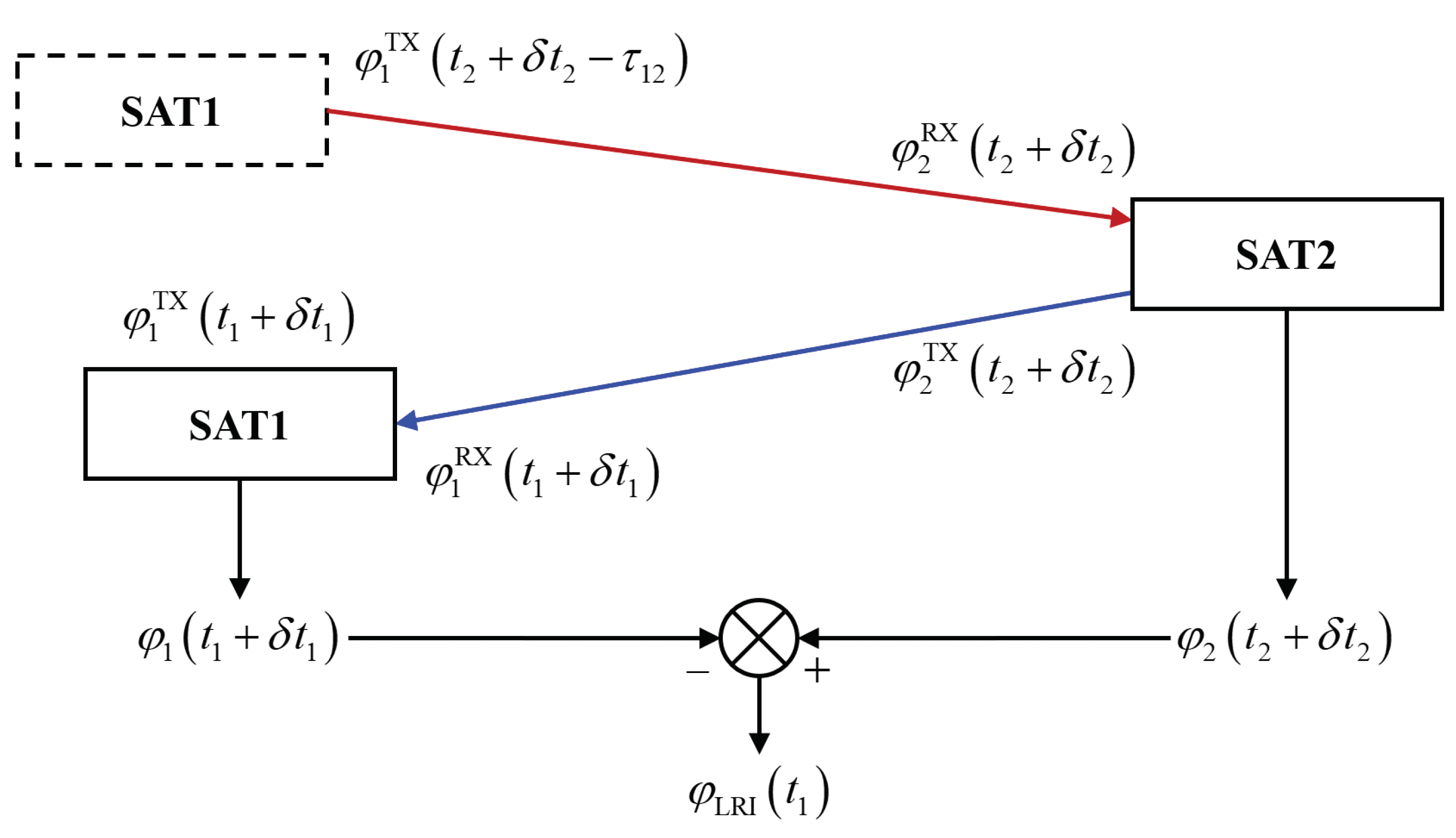
Figure 2 shows the phase observables of the two satellites at the actual time and their combinations φ LRI ( t 1 ) . The light (red line) from the master (SAT1 with a dashed border) arrives at the transponder (SAT2 with a solid border) after a travel time τ 12 . Similarly, the light (blue line) from the transponder arrives at the master (SAT1 with a solid border) after a travel time τ 21 . The time-of-flight (TOF) τ 12 and τ 21 can be precisely calculated with an iteration process [24]. The nominal time t 1 and t 2 satisfy the equation
t 2 = t 1 τ 21 .
The cumulated phase of RX light is equal to the phase of the corresponding TX light at the transmitting time, i.e.,
φ 1 RX ( t 1 + δ t 1 ) = φ 2 TX ( t 1 + δ t 1 τ 21 ) , φ 2 RX ( t 2 + δ t 2 ) = φ 1 TX ( t 2 + δ t 2 τ 12 ) .
Due to the frequency offset introduced in the OPLL, the phase of interference light in SAT2 increases fast as a ramp, the slope of which is roughly + 10 MHz . By writing the OPLL phase contributions as φ 2 OPLL , the phase of the TX light in SAT2 can be expressed as
φ 2 TX ( t 2 + δ t 2 ) = φ 2 OPLL ( t 2 + δ t 2 ) + φ 2 RX ( t 2 + δ t 2 ) .
Substituting Equations (3)–(5) into Equation (2) yields
φ 1 ( t 1 + δ t 1 ) = φ 1 TX ( t 1 + δ t 1 τ 21 τ 12 ) + φ 2 OPLL ( t 1 + δ t 1 τ 21 ) φ 1 TX ( t 1 + δ t 1 ) N 1 ε 1 , φ 2 ( t 2 + δ t 2 ) = φ 2 OPLL ( t 1 + δ t 2 τ 21 ) + N 2 + ε 2 .
The two-way ranging phase of LRI at nominal time t 1 is computed as the difference of the transponder and master phase:
φ LRI ( t 1 ) = φ 2 ( t 2 + δ t 2 ) φ 1 ( t 1 + δ t 1 ) .
By substituting Equation (6) into Equation (7) and applying the Taylor expansion since the light travel time and time tag error are small, we have
φ LRI ( t 1 ) f 1 ( τ 12 + τ 21 ) + f OPLL ( δ t 2 δ t 1 ) + ( N 1 + N 2 ) + ( ε 1 + ε 2 ) ,
where f 1 and f OPLL represent the master laser frequency and the heterodyne frequency in the OPLL, respectively. Each frequency can be divided into a constant part f ¯ and a tiny variable part δ f . Therefore, one can write
f 1 = f ¯ 1 + δ f 1 , f OPLL = f ¯ OPLL + δ f OPLL .
The two-way ranging phase is then written as
φ LRI ( t 1 ) f ¯ 1 ( τ 12 + τ 21 ) + δ f 1 ( τ 12 + τ 21 ) + f ¯ OPLL ( δ t 2 δ t 1 ) + δ f OPLL ( δ t 2 δ t 1 ) + ( N 1 + N 2 ) + ( ε 1 + ε 2 ) ,
the unit of which can be converted from cycle to meter by using the nominal laser frequency f 0 . Therefore, the one-way range ρ LRI with the unit of meter reads
ρ LRI ( t 1 ) = c 2 f 0 φ LRI ( t 1 ) c f ¯ 1 2 f 0 ( τ 12 + τ 21 ) + c δ f 1 2 f 0 ( τ 12 + τ 21 ) + c f ¯ OPLL 2 f 0 ( δ t 2 δ t 1 ) + c δ f OPLL 2 f 0 ( δ t 2 δ t 1 ) + c 2 f 0 ( N 1 + N 2 ) + c 2 f 0 ( ε 1 + ε 2 ) .
For gravity field recovery, the measured range needs to be converted into the instantaneous range between satellites, which means the distance between two satellite positions at exactly the same time. Here, we use ρ inst to represent the instantaneous range and we define an equivalent light time τ corresponding to the instantaneous range as τ = ρ inst / c , where c denotes the speed of light in a vacuum. The first two terms in Equation (11) can then be written as
c f ¯ 1 2 f 0 ( τ 12 + τ 21 ) + c δ f 1 2 f 0 ( τ 12 + τ 21 ) = f ¯ 1 f 0 ρ inst + f ¯ 1 f 0 δ ρ path + δ f 1 f 0 ρ inst + δ f 1 f 0 δ ρ path ,
where the pathlength error δ ρ path due to the non-zero light travel time is defined as
δ ρ path = c ( τ 12 + τ 21 ) 2 τ .
By dropping the small terms in Equations (11) and (12), the intersatellite range measurement can be written as
ρ LRI ( t 1 ) f ¯ 1 f 0 ρ inst + f ¯ 1 f 0 δ ρ path + δ f 1 f 0 ρ inst + c f ¯ OPLL 2 f 0 ( δ t 2 δ t 1 ) + c 2 f 0 ( N 1 + N 2 ) + c 2 f 0 ( ε 1 + ε 2 ) ,
where the first term on the right-hand side is the scaled value of the instantaneous range, the second term corresponds to the pathlength error due to time delays, the third term is caused by the laser frequency noise and is scaled by the range, the fourth term is due to the time tag error, the fifth term represents a constant bias, for which the measured range is called the biased range, and the last term is due to the phase readout noise. The instantaneous range in the first term is scaled for the reason that there is a small difference between the nominal laser frequency f 0 and the actual constant part of the laser frequency f ¯ 1 in flight. Since the cavity is unable to provide information of f ¯ 1 , if there is no other method to obtain it in orbit, a scaled factor s close to one will be estimated [21], i.e.,
s = 1 + α f 0 f ¯ 1 ,
where α is of the order of 10 6 for the GRACE-FO mission and is provided in the RL04 LRI1B data product. After applying the scale correction, the measured biased range reads
ρ LRI ( t 1 ) ρ inst + δ ρ path + δ f 1 f ¯ 1 ρ inst + c f ¯ OPLL 2 f ¯ 1 ( δ t 2 δ t 1 ) + c 2 f ¯ 1 ( N 1 + N 2 ) + c 2 f ¯ 1 ( ε 1 + ε 2 ) .
Since the influence of the scale factor is beyond the scope of this paper and is not important to the study here, we assume that we have obtained the value of f ¯ 1 in orbit and, thus, there is no need to estimate the scale factor in the following sections. The pathlength error δ ρ path consists of all the physical effects related to the light path, including the delays due to media, TTL coupling, and relativistic effects [25], and one should correct it by applying the so-called light time correction (LTC), taking all these effects into account. In practice, however, the light time correction is usually calculated without considering the TTL coupling, and an additional TTL correction term is estimated individually. In the GRACE-FO RL04 KBR1B data product, the light time correction and the antenna offset correction, which is referred to as the TTL correction for KBR, are provided separately in two columns. The TTL correction in the GRACE-FO RL04 LRI1B data product is set to zero since it is much smaller than the one for KBR and can be omitted. Therefore, we have
δ ρ path δ ρ TOF + δ ρ TTL δ ρ LTC δ ρ TTLC
where δ ρ TOF denotes the time-of-flight effect including the pathlength error due to media and relativistic effects; δ ρ TTL denotes the TTL coupling error; δ ρ LTC and δ ρ TTLC denote the estimated light time correction and the TTL correction, respectively. Once the light time correction term and the TTL correction term are estimated, we can obtain the corrected biased range [13]
ρ corr ( t 1 ) = ρ LRI ( t 1 ) + δ ρ LTC + δ ρ TTLC ρ inst + δ f 1 f ¯ 1 ρ inst + c f ¯ OPLL 2 f ¯ 1 ( δ t 2 δ t 1 ) + c 2 f ¯ 1 ( N 1 + N 2 ) + c 2 f ¯ 1 ( ε 1 + ε 2 ) ,
which is one of the inputs to the gravity field recovery.

4. TTL Model

This section provides a model for TTL coupling due to the CM-VP offset, which is similar to the work in [14]. For the sake of clarity, Equation (16) can be rewritten as
ρ LRI = ρ inst + δ ρ TTL + δ ρ others ,
where δ ρ others denotes the contributions of all other error sources.
As shown in Figure 3, we use the subscript i ( i = 1 , 2 ) to indicate the SAT1 and SAT2. The measured range can be regarded as the distance of V P 1 and V P 2 with additional bias and noise, and the instantaneous range is the distance between C M 1 and C M 2 of the two satellites. Therefore, we have
ρ LRI = | V P 2 V P 1 | + δ ρ others , ρ inst = | C M 2 C M 1 | .
The TTL error term is then expressed as
δ ρ TTL = ρ LRI ρ inst δ ρ others = | V P 2 V P 1 | | C M 2 C M 1 | | P 2 P 1 | | C M 2 C M 1 | = e LOS , 1 · V 1 e LOS , 2 · V 2 ,
where the approximation | V P 2 V P 1 | | P 2 P 1 | is applied since the distance between V P i and P i ( i = 1 , 2 ) is much smaller than the distance between V P 1 and V P 2 . The absolute value of the TTL error of each satellite is approximately the projection of the vector V i on the line of sight (LOS). One can compute the TTL error in the line-of-sight frame (LOSF) shown in Figure 3 for each satellite:
δ ρ TTL , i e LOS , i LOSF i · V i LOSF i = 1 0 0 · V i LOSF i ,
where the superscripts denote the frames of the vectors. Since the V P i co-rotates with the satellite around the C M i , the components of the vector V i SF i = ( Δ x i , Δ y i , Δ z i ) T expressed in the satellite frame (SF) for each satellite remain unchanged, unless a disturbance to the center of mass (e.g., a mass trim maneuver aimed at moving the center of mass back to the ACC reference point [14]) happens. With the rotation matrix R SF LOSF , which denotes the rotation transforming a vector from SF to LOSF, we have
δ ρ TTL , i 1 0 0 · R SF i LOSF i V i SF i .
The roll angle θ x , pitch angle θ z , and yaw angle θ z used in this paper are defined by
R SF LOSF = R x ( θ x ) R y ( θ y ) R z ( θ z ) = c y c z c y s z s y s x s y c z c x s z s x s y s z c x c z s x c y c x s y c z s x s z c x s y s z s x c z c x c y ,
where c i = cos θ i , s i = sin θ i , i = x , y , z ; the matrices R x ( θ x ) , R y ( θ y ) and R z ( θ z ) denote the rotations around the x-, y- and z-axes by angles θ x , θ y , and θ z , respectively. Substitution of Equation (24) into Equation (23) yields
δ ρ TTL , i c y c z Δ x c y s z Δ y + s y Δ z ,
where the index i on the right-hand side is dropped. Since the angles are small, Taylor expansion can be applied. In general, terms with order higher than two are omitted; thus, we have
δ ρ TTL , i 1 2 θ y 2 + 1 2 θ z 2 Δ x θ z Δ y + θ y Δ z Δ x ,
where we find Δ x / 2 is the quadratic coupling factor of the pitch and yaw angles, Δ y is the linear coupling factor of the yaw angle, and Δ z is the linear coupling factor of the pitch angle. The constant term is not important to the biased range. With the subscript 1 and 2 indicating the SAT1 and SAT2, respectively, the total TTL error of the two satellites reads
δ ρ TTL 1 2 θ y , 1 2 + 1 2 θ z , 1 2 Δ x 1 θ z , 1 Δ y 1 + θ y , 1 Δ z 1 Δ x 1 + 1 2 θ y , 2 2 + 1 2 θ z , 2 2 Δ x 2 θ z , 2 Δ y 2 + θ y , 2 Δ z 2 Δ x 2 .
In the case that Δ x i ( i = 1 , 2 ) is small, like the GRACE-FO LRI, the quadratic coupling terms can be omitted [14], i.e.,
δ ρ TTL θ z , 1 Δ y 1 + θ y , 1 Δ z 1 Δ x 1 θ z , 2 Δ y 2 + θ y , 2 Δ z 2 Δ x 2 .
In practice, the pointing angles we use for TTL coupling estimation are measured ones, which unavoidably contain biases and noise. A static angle offset is irrelevant for the linear coupling TTL error since it only introduces an additional constant term, which is not important as mentioned above. However, taking the quadratic coupling terms into account, additional linear terms appear in the expression of the TTL error because of the biased angles. In this situation, the TTL error for each satellite reads
δ ρ TTL , i 1 2 θ y , i 2 + 1 2 θ z , i 2 Δ x i θ z , i Δ y i + θ y , i Δ z i Δ x i 1 2 θ ^ y , i Δ θ y , i 2 + 1 2 θ ^ z , i Δ θ z , i 2 Δ x i θ ^ z , i Δ θ z , i Δ y i + θ ^ y , i Δ θ y , i Δ z i Δ x i = 1 2 θ ^ y , i 2 + 1 2 θ ^ z , i 2 Δ x i + θ ^ z , i ( Δ θ z , i Δ x i Δ y i ) + θ ^ y , i ( Δ θ y , i Δ x i + Δ z i ) + Δ θ z , i Δ y i Δ θ y , i Δ z i Δ x i ,
where θ ^ y , i and θ ^ z , i denote the measured pitch and yaw angles and Δ θ y , i and Δ θ z , i denote the pitch and yaw angle biases between the measured and the true angles, respectively, and they satisfy the equations θ ^ y , i θ y , i + Δ θ y , i and θ ^ z , i θ z , i + Δ θ z , i . The additional linear terms are in direct proportion to Δ x i and the angle biases. These terms can be omitted when Δ x i is not a large number since the largest angle biases are roughly of the order of 10 3 rad. In contrast, the estimated linear TTL coupling factors will be apparently affected when Δ x i is up to 1 m. The least squares method is used for TTL coupling estimation in this paper. Six coupling factors { p x , 1 , p y , 1 , p z , 1 , p x , 2 , p y , 2 , p z , 2 } can be estimated according to Equation (29) and the desired values are { Δ x 1 , Δ y 1 , Δ z 1 , Δ x 2 , Δ y 2 , Δ z 2 } in the case with zero angle biases.
As mentioned in Section 1, a band-pass filter is applied to the LRI range and the pointing angles in the estimation process, which yields
BPF ( ρ LRI ) = BPF ( ρ inst ) + BPF ( δ ρ TTL ) + BPF ( δ ρ others ) BPF ( δ ρ NG ) + BPF ( δ ρ TTL ) + BPF ( δ ρ LF ) ,
where the operator BPF refers to the band-pass filter. As an example, the cutoff frequencies are 40 mHz and 175 mHz in [10]. The band-pass-filtered instantaneous range is dominated by the term δ ρ NG caused by the non-gravitational forces. δ ρ LF , the contribution of the laser frequency noise, expressed as ρ inst · δ f 1 / f ¯ 1 according to Equation (16), is the main error term of the band-pass-filtered δ ρ others . If the band-pass-filtered TTL error δ ρ TTL is significantly greater than the other two terms (e.g., a specific calibration maneuver has been performed), then we can directly use the following equation for TTL estimation:
BPF ( ρ LRI ) = BPF ( δ ρ TTL ) + ϵ err
where ϵ err is the small error term. The expression of TTL error is given in Equation (27). In general, the TTL error at the passband is probably lower than the terms of the non-gravitational forces or the laser frequency noise. As shown in Figure 4, the TTL error of GRACE-FO (green) is relatively small compared to the ranging signal and even lower than the laser frequency noise (red) at high frequencies. In the situation that the CM-VP offset in each satellite is set to 1.5 m, the TTL error may reach the level of the ranging signal at frequencies above 30 mHz, which is conducive to parameter estimation.
Considering that the ranging signal induced by non-gravitational forces can be calculated from accelerometer measurements of both satellites by integrating the differential linear accelerations on the LOS twice, one can rewrite the observation equation as
BPF ( ρ LRI δ ρ NG ) BPF ρ LRI ( a LOS , 1 a LOS , 2 ) d t = BPF ( δ ρ TTL ) + ϵ err
in which a LOS , i ( i = 1 , 2 ) denotes the projection of the measured linear accelerations on the LOS for SATi. The enlarged low-frequency error due to the integration, as well as the constant terms, are filtered out. Equation (32) is used for the TTL estimation in this research.
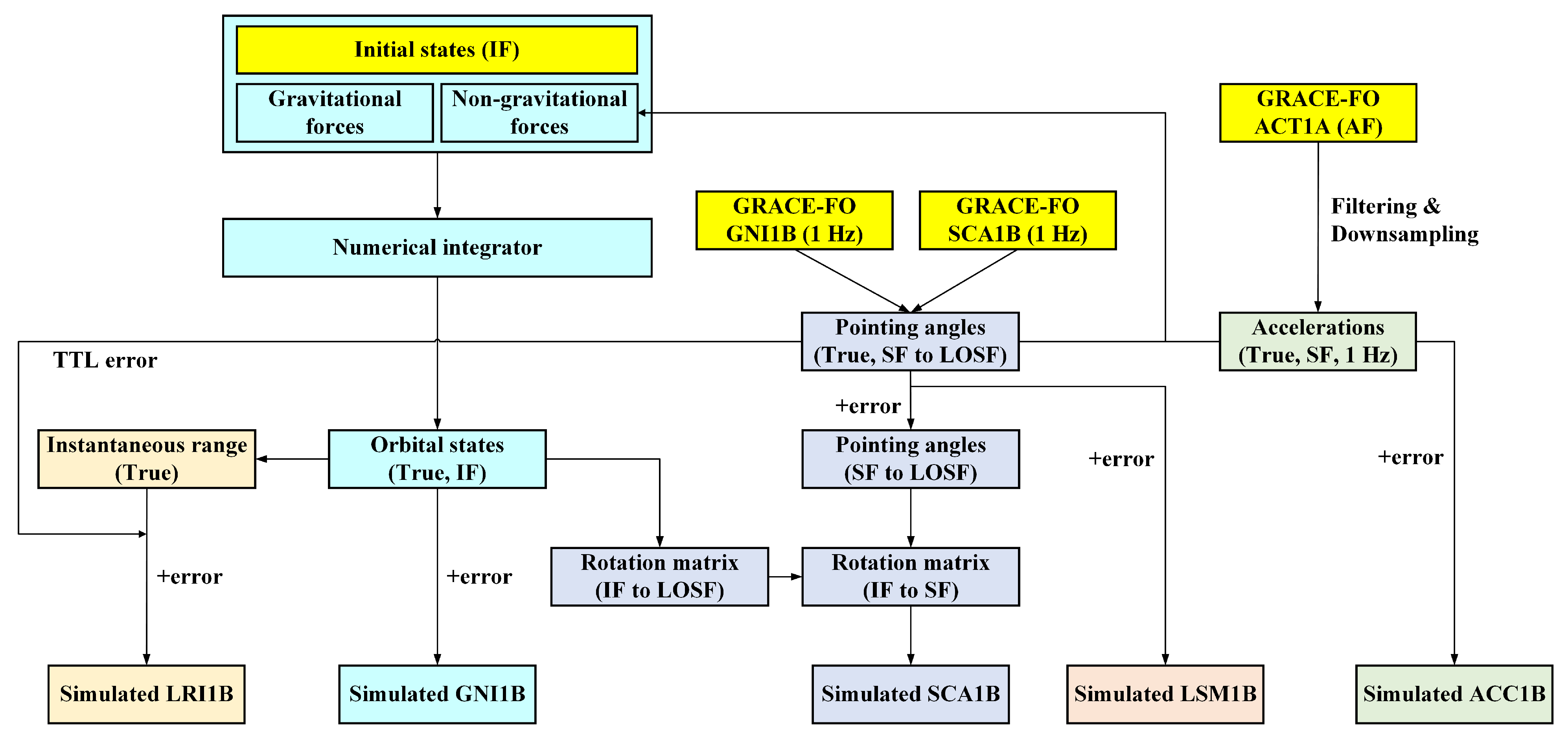
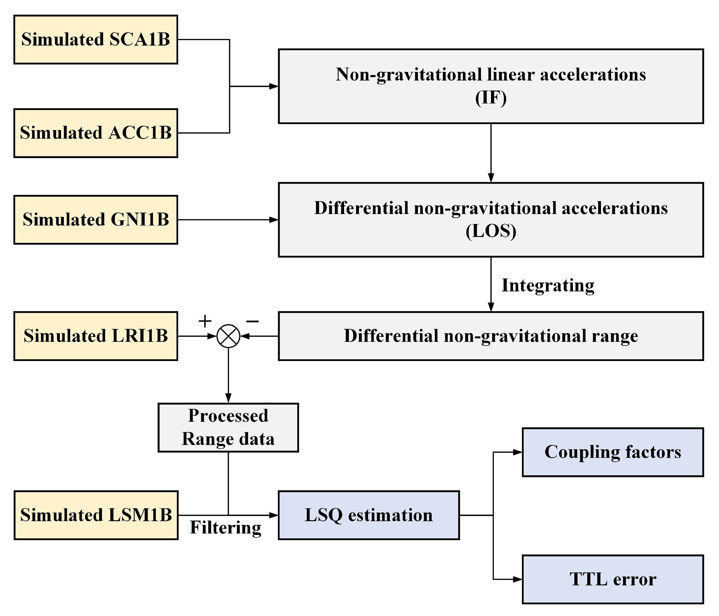
5. Data Simulation

A numerical simulation was performed to investigate under what conditions we can estimate the TTL error without any specific calibration maneuvers for it. Five types of data (GNI1B, SCA1B, ACC1B, LRI1B, LSM1B) were generated:
  • Simulated GNI1B—GNSS navigation data in terms of trajectory states consisting of satellite positions and velocities in an inertial frame (IF);
  • Simulated SCA1B—star camera assembly (SCA) measurements in terms of quaternions, describing the relationship between the inertial frame and the satellite frame;
  • Simulated ACC1B—linear non-gravitational acceleration measurements in the satellite frame;
  • Simulated LRI1B—biased range, range rate, and range acceleration data;
  • Simulated LSM1B—LRI steering mirror measurements in terms of the pitch and yaw pointing angles, which were used in the TTL estimation process.
We chose the International Celestial Reference Frame (ICRF) as the inertial frame. A flowchart of the data simulation procedure is shown in Figure 5. Similarly to [27], after the error-free observations were calculated, the error terms were added up to generate the simulated measurements.

5.1. GNI1B Simulation

Simulated orbital data with a period of one day were used for the TTL estimation. The initial states are taken from the official GRACE-FO GNI1B data and the corresponding time is 23:55:00 on 31 March 2021 in GPS time. The initial orbital elements are listed in Table 1. The gravitational and non-gravitational force models we used for orbit integration are listed in Table 2. The 12th order Gauss–Jackson integrator was used for orbit integration and the step-size was 1 second.
The models in forward procedure in Table 2 were used to generate the error-free orbital states, while the models in the POD procedure were applied to generate the simulated GNI1B data that contain errors. The error-free orbital states were used as observations for the POD procedure since there was no direct simulation of GNSS measurements. The root mean square (RMS) values of the position and velocity residuals were set to several centimeters and tens of microns per second, respectively, by controlling the iteration times in the POD procedure, in which the initial states, the accelerometer scale, and the bias parameters were estimated.

5.2. SCA1B Simulation

The official GRACE-FO SCA1B data provide rotation quaternions from the inertial frame to the satellite frame. The matrix rotating from IF to SF can be derived from the quaternions:
R IF SF = q 0 2 + q 1 2 q 2 2 q 3 2 2 ( q 1 q 2 + q 0 q 3 ) 2 ( q 1 q 3 q 0 q 2 ) 2 ( q 1 q 2 q 0 q 3 ) q 0 2 q 1 2 + q 2 2 q 3 2 2 ( q 2 q 3 + q 0 q 1 ) 2 ( q 1 q 3 + q 0 q 2 ) 2 ( q 2 q 3 q 0 q 1 ) q 0 2 q 1 2 q 2 2 + q 3 2 ,
where q = ( q 0 , q 1 , q 2 , q 3 ) represents the quaternions. In order to calculate the pointing angles, the rotation matrix from IF to LOSF is needed, which can be written as
R IF LOSF = e LOSF , x e LOSF , y e LOSF , z T .
Taking SAT1 as an example, the axes of LOSF in Equation (34) are defined as
e LOSF 1 , x = r 2 r 1 | r 2 r 1 | , e LOSF 1 , y = e LOSF 1 , x × r 1 | e LOSF 1 , x × r 1 | , e LOSF 1 , z = e LOSF 1 , x × e LOSF 1 , y ,
where r 1 and r 2 represent the position vectors of SAT1 and SAT2 in the inertial frame, respectively. The indices 1 and 2 in Equation (35) should be exchanged for SAT2. For the GRACE-FO mission, the inertial position vectors can be found in the GNI1B data. Then the rotation matrix from SF to LOSF reads
R SF LOSF = R IF LOSF R IF SF T .
The pointing angles can then be computed as
θ x = arctan R 23 R 33 , θ y = arcsin R 13 , θ z = arctan R 12 R 11 ,
where R i j represents the entry in row i and column j of R SF LOSF . The pointing angles calculated from the GRACE-FO GNI1B and SCA1B data are considered to be error-free and were converted into the rotation matrix transforming the non-gravitational accelerations from SF to IF with the calculated trajectory states. These pointing angles were also used to compute the true TTL error, which was then added to the instantaneous range. Random noise added to the pointing angles was generated based on the following formula:
ASD [ δ θ SCA 1 B ] ( f ) = 2 × 10 4 rad / Hz 1 / 2 × 1 + f 1 mHz 1 .
This formula is an approximation of the difference between the pointing angles calculated from the official SCA1B and LSM1B in terms of the amplitude spectral density. The LSM1B data provide the pitch and yaw pointing angles measured by the FSM, whose noise is considered as white noise with a level of a few μ rad / Hz 1 / 2 , which is apparently lower than that of SCA1B at frequencies below 50 mHz [28]. Therefore, it is considered that the difference between the two types of data at low frequencies is mainly due to the noise from SCA1B. So, Equation (38) was used to generate the pointing angle noise for the simulated SCA1B data. The method we used to generate the time domain data satisfying the required PSD or ASD is described in [29]. Although roll angle measurement is not included in LSM1B data, Equation (38) was still applied to the noise generation for roll angles together with the pitch and yaw angles in this study. In addition, biases with values of several hundreds of μ rad were added to the pointing angles. After that, the rotation matrix R IF SF was recalculated using the pointing angles with error. Then, the simulated SCA1B data in terms of quaternions could be computed. To avoid numerical instability, the way we compute quaternions from a given rotation matrix is based on the pseudocode provided in [27] with some adjustments.
In the GRACE-FO mission, the SCA1B data are produced by an optimal combination of the measurements from the star camera assembly and the inertial measurement unit (IMU). The IMU data are used to lower the angle noise at high frequencies. Nonetheless, the LSM1B data are preferred for the TTL estimation in this study due to their low noise in a wide frequency range.

5.3. ACC1B Simulation

The official GRACE-FO ACT1A data contain roughly 10 Hz linear acceleration measurements of the ACC proof mass in a frame called the accelerometer frame (AF) whose axes are defined as
e AF , x = + e SF , y , e AF , y = + e SF , z , e AF , z = + e SF , x .
The raw ACT1A data were low-pass filtered with a cutoff frequency at 0.5 Hz and downsampled to 1 Hz to remove some high-frequency noise. The new ACT1A data were then expressed in the satellite frame according to Equation (39) as the error-free data of the non-gravitational accelerations. Invariant scale and bias parameters were used in the simulation. The ASD noise models we used to generate the accelerometer noise for the simulated ACC1B data read
ASD [ δ a ACC 1 B , SF , y ] ( f ) = 10 9 m / s 2 / Hz 1 / 2 × 1 + f 0.5 Hz 4 + f 0.1 Hz 1 , ASD [ δ a ACC 1 B , SF , x / z ] ( f ) = 10 10 m / s 2 / Hz 1 / 2 × 1 + f 0.5 Hz 4 + f 0.005 Hz 1 ,
which is referenced from [4]. The generated time domain noise data were then added to the error-free values.

5.4. LRI1B Simulation

The true instantaneous range can be directly computed from the error-free orbital states as
ρ inst = ( r 2 r 1 ) · ( r 2 r 1 ) .
For the simulation of ranging data, Equation (16) can be rewritten as
ρ LRI ( t 1 ) ρ inst + Δ ρ bias + δ ρ TOF + δ ρ TTL + δ ρ LF + δ ρ timetag + δ ρ readout ,
where Δ ρ bias is a constant denoting the measurement bias; δ ρ TOF denotes the error induced by the time delays due to media and relativistic effects; δ ρ TTL and δ ρ LF denote the error caused by the tilt-to-length coupling and laser frequency instability mentioned in Section 4, respectively; δ ρ timetag denotes the range error due to the time tag error; and δ ρ readout denotes the range error due to the phase readout noise. After adding the range error, the simulated range rate and the range acceleration can be obtained by applying the CRN filter [30]. The ASD of the instantaneous range and the non-constant error terms are shown in Figure 6. Descriptions of the error terms are as provided below.

5.4.1. TOF Effect

Due to the non-zero travel time of the light between the two satellites, the measured range always deviates from the instantaneous range. The range deviation due to media and relativistic effects is a systematic error called the time-of-flight (TOF) effect in Section 3, which can be calculated in an iteration process. In the simulation, we used the analytical expressions in [25] and the error-free orbital data to calculate this error (green trace in Figure 6) during the forward procedure and added it to the error-free instantaneous range. The corresponding light time correction term δ ρ LTC mentioned in Section 3 can be calculated using the simulated GNI1B data with error during the POD procedure though it was not used in the TTL estimation process and has an opposite sign:
δ ρ LTC δ ρ TOF .

5.4.2. TTL Error

The TTL error is mainly caused by the CM-VP offset. As long as the components of the offset vector in satellite frame (i.e., Δ x , Δ y , and Δ z ) for each satellite are provided, the TTL error can be computed using Equation (25) with the error-free pointing angles. The total TTL error of the two satellites (magenta trace in Figure 6 as an example, assuming Δ x = 1.5 m and Δ y = Δ z = 0.5 mm for each satellite) was then added to the instantaneous range. The corresponding TTL correction term, also named the vertex point correction (VPC) term here, was estimated based on Equation (27) using the range and angle data with error and has an opposite sign:
δ ρ TTLC δ ρ VPC δ ρ TTL .

5.4.3. Laser Frequency Error

The master (SAT1) laser frequency can be divided into three parts, as shown in the following equation [31,32]:
f 1 = f ¯ 1 + δ f 1 f ¯ 1 + Φ ( r 1 ) Φ 0 c 2 1 2 v 2 c 2 f ¯ 1 + δ f cav ,
where f ¯ 1 281.6 THz and the last two terms represent the frequency error due to the relativistic effects and the cavity instability, respectively; Φ ( r 1 ) denotes the Newtonian gravitational potential at the position of SAT1 carrying a negative sign, and Φ 0 at the geoid including the centripetal potential caused by the Earth’s rotation. Φ ( r 1 ) can be calculated using the gravitational force models during the forward procedure, while the absolute value of the constant Φ 0 / c 2 equals the scale difference L G between the terrestrial time (TT) and the geocentric coordinate time (TCG):
Φ 0 c 2 = L G = 6.969290134 × 10 10 .
The term δ f cav ( t ) was generated according to Equation (1). The range error induced by the laser frequency variability can be computed as
δ ρ LF = δ f 1 f ¯ 1 ρ inst .
The ASD of δ ρ LF is shown in red in both Figure 4 and Figure 6.

5.4.4. Time Tag Error

The LRI time is realized by the onboard ultrastable oscillator (USO) for each satellite. Since the USO time is different from the GNSS time due to the clock rate difference, a time tag correction term t ε provided in the CLK1B data product is needed to convert the LRI time tags to GNSS time tags (it is more complicated for the LRI in GRACE-FO: the LRI time is first converted to the onboard computer (OBC) time using the datation reports; then the TIM1B data product provides the time tag difference between the OBC time and the instrument processing unit (IPU) receiver time; finally, the CLK1B data product is used to convert the IPU receiver time to the GPS time). After applying the time tag correction, the residual time tag error is dominated by the error from the GNSS POD and clock solution. We used the following ASD model to simulate the error of t ε for each satellite [32]:
ASD [ δ t ε ] ( f ) = 1.5 mm / Hz 1 / 2 c × f 1 Hz 1 / 2 + 10 μ m / Hz 1 / 2 c × f 1 Hz 5 / 4 .
This model is an approximation of the clock measurement noise in the Deep Space Atomic Clock (DSAC) mission [33]. Furthermore, to form a two-way phase observation, the transponder (SAT2) phase, whose time tags already contain the CLK1B time tag error δ t ε , 2 , is required to interpolate the time tag to t 2 = t 1 τ 21 , indicating that the error of light travel time τ 21 determined by the POD also induces a time tag error, which was not mentioned in [32]. The time-of-flight τ 21 can be obtained in the calculation process of the TOF effect and LTC mentioned in Section 5.4.1. Based on the discussion, we have
δ t 1 = δ t ε , 1 , δ t 2 = δ t ε , 2 δ τ 21 ,
where δ t ε , 1 and δ t ε , 2 were generated according to Equation (48), and δ τ 21 represents the TOF (from transponder to master) difference between the calculation results from the POD and forward procedure. The range error caused by the time tag error (cyan trace in Figure 6) can be computed as
δ ρ timetag = c f ¯ OPLL 2 f ¯ 1 ( δ t 2 δ t 1 ) .
where f ¯ OPLL 10 MHz .

5.4.5. Phase Readout Noise

The phase readout noise can be computed with the carrier-to-noise ratio (CNR). The ASD model of the readout noise reads
ASD [ ε ] ( f ) = 1 rad × 1 CNR = 1 2 π cycles × 1 CNR .
where the CNR was set to 80 dBHz for each satellite in the simulation. The range error due to the readout noise (yellow trace in Figure 6) reads
δ ρ readout = c 2 f ¯ 1 ( ε 1 + ε 2 ) .
where the time domain phase readout noise ε 1 and ε 2 in cycles were generated according to Equation (51).

5.5. LSM1B Simulation

The simulated LSM1B data contain only the pitch and yaw angles since the FSM is not sensitive to the roll angles. The data were derived from the error-free pointing angles by adding biases of several hundreds of μ rad and some white noise. The noise level could be changed during the investigation of the TTL parameter estimation.

6. TTL Estimation

The five types of data mentioned in Section 5 are used for TTL estimation as shown in Figure 7. The simulated SCA1B data are used to rotate the simulated ACC1B measurements from SF to IF. Then, the simulated GNI1B was used to calculate the differential non-gravitational accelerations on the LOS. After integrating twice, the generated differential non-gravitational range was subtracted from the simulated LRI1B range data, as shown in Equation (32). The processed range data were then band-pass-filtered together with the simulated LSM1B angles and the LSQ estimation was performed to obtain the values of the coupling factors and the TTL error. The cutoff frequencies of the band-pass filter were set to 50 and 100 mHz in the estimation process.
The impact of different conditions, including the CM-VP offset, the pointing angle noise, and the laser frequency noise for TTL estimation, was investigated. We divide the results into two types: results under the S-type longitudinal offset (i.e., Δ x = 0.5 mm , like the small CM-VP offset of GRACE-FO’s LRI) and the results under the L-type longitudinal offset (i.e., Δ x = 1.5 m , like the large CM-APC offset of KBR). The difference between the estimated and the true value should be lower than the GRACE-FO’s TTL error for successful TTL estimation.

6.1. Results under S-Type Offset

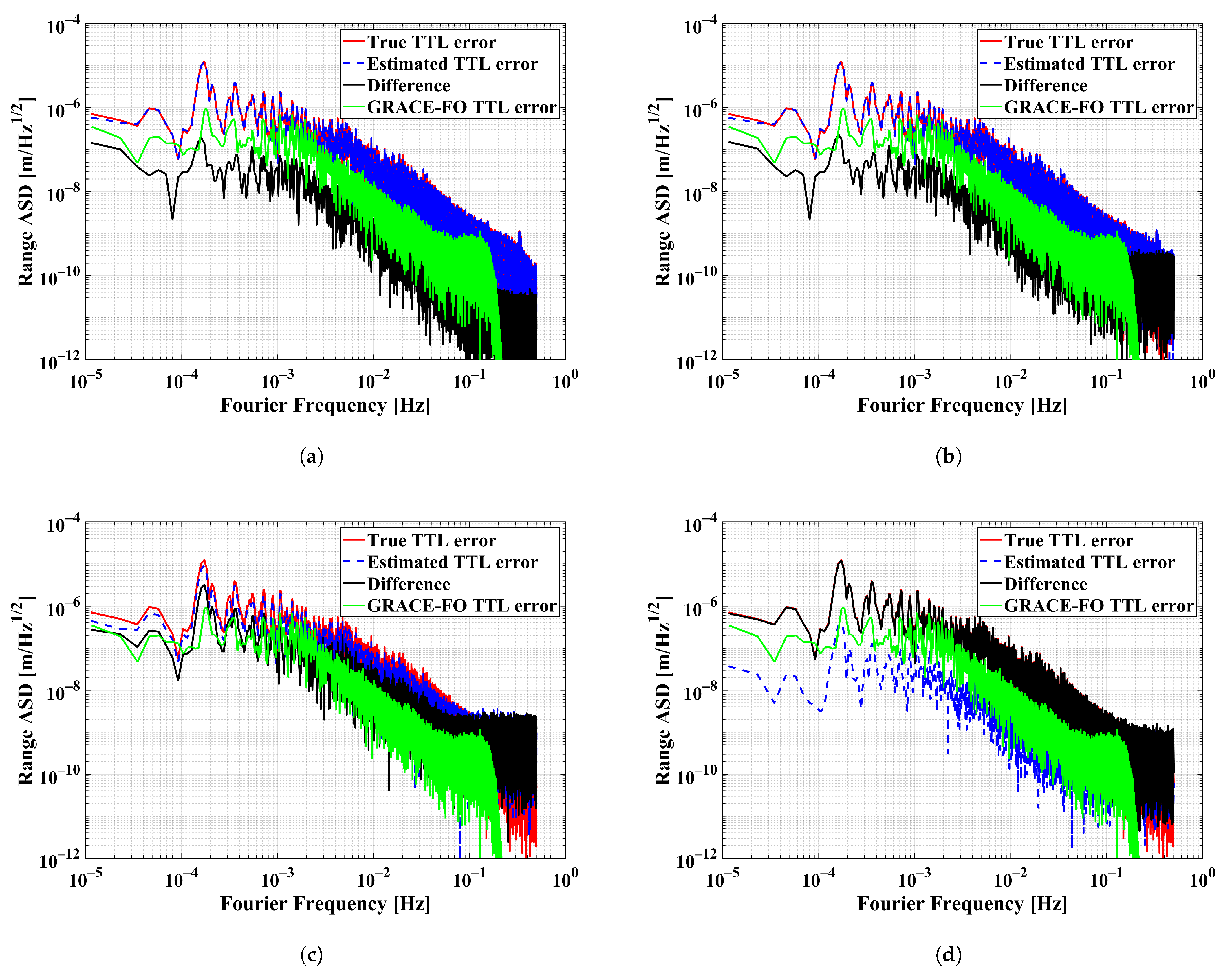
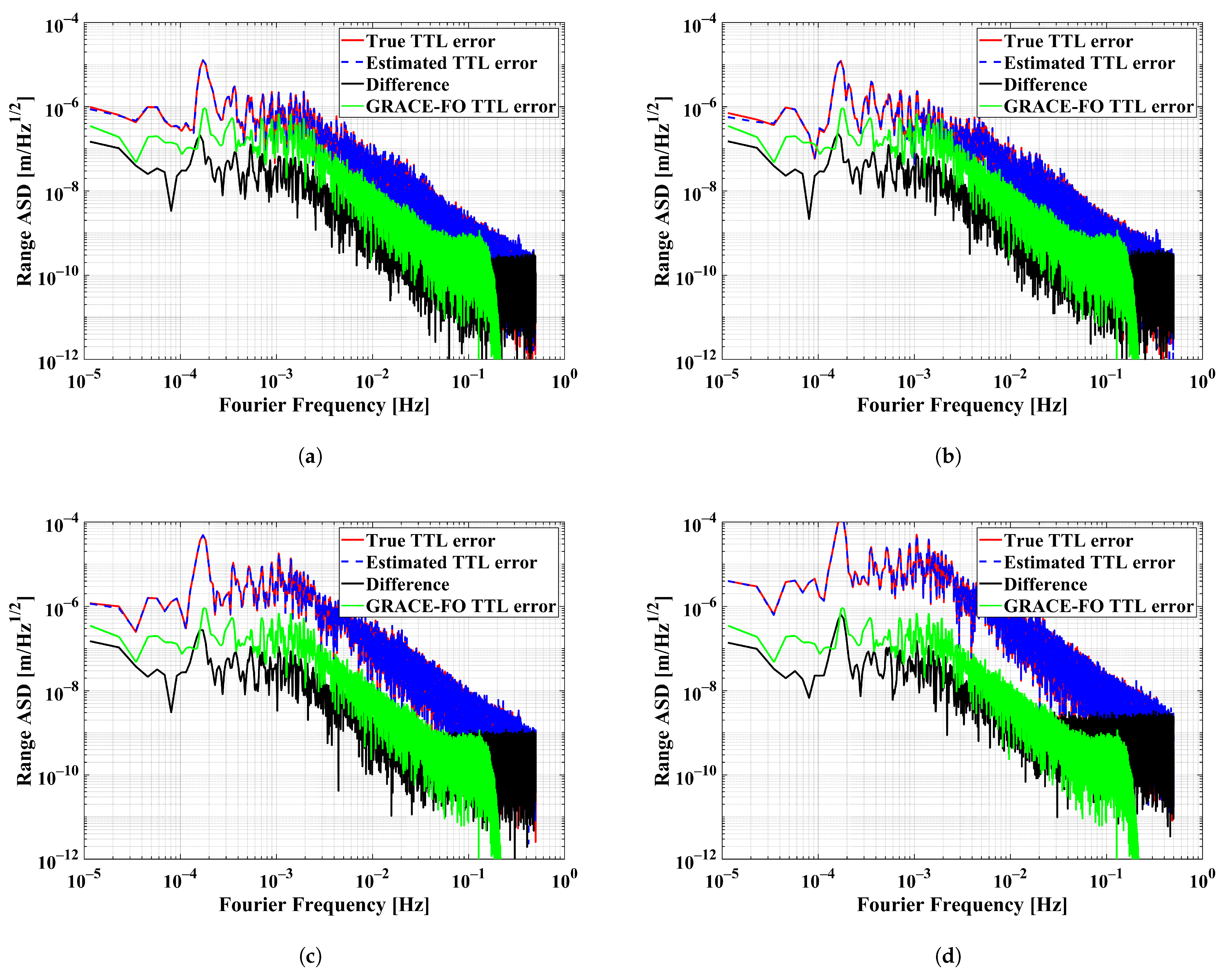
6.1.1. Impact of Pointing Angle Noise

Assuming Δ x = Δ y = Δ z = 0.5 mm for each satellite, the impact under different noise levels of pointing angle measurement was tested in the TTL estimation. Only four linear coupling factors { p y , 1 , p z , 1 , p y , 2 , p z , 2 } were estimated.
The ASD of the input and estimated TTL error are shown in red and blue, respectively, in Figure 8. In the cases that white noise with levels of 0.01 μ rad / Hz 1 / 2 and 0.1 μ rad / Hz 1 / 2 were added to the pointing angles, the estimation errors shown in black are similar, which can also be seen in Table 3, where the estimated coupling factors are at the same level. In case (c), the angle noise level is similar to that of the GRACE-FO LSM1B data and the estimation error is a bit higher than the TTL error of GRACE-FO (green). When the angle noise is up to the level of 10 μ rad / Hz 1 / 2 , poor estimation results can be seen. One can notice that the estimation errors at high frequencies are limited by the white angle noise instead of the estimation error of the coupling factors. It can be concluded that the noise of the angle measurement should be better than 1 μ rad / Hz 1 / 2 for successful TTL estimation.

6.1.2. Impact of Lateral Offset

Keeping the longitudinal offsets unchanged as in the previous subsection, the impact of different lateral offsets is shown in Figure 9 and Table 4 in the case that the pointing angle noise level was set to 0.1 μ rad / Hz 1 / 2 . As the lateral offsets increase, the true TTL error (red) grows and so does the estimation error (black) at high frequencies, which are limited by the white angle noise, while the estimation error at low frequencies does not significantly change. Considering that the high frequency noise can be filtered out, the lateral offset is not a strict condition in the case of 0.1 μ rad / Hz 1 / 2 angle noise from the perspective of TTL estimation in this study.

6.1.3. Impact of Laser Frequency Noise

The laser frequency noise generated by 1 and 10 times the ASD model (cf. Equation (1)) was tested for TTL estimation with Δ x = Δ y = Δ z = 0.5 mm for each satellite and 0.1 μ rad / Hz 1 / 2 white angle noise. As shown in Figure 10 and Table 5, the laser frequency noise in case (b) is 10 times that in case (a), and as a result, the estimation error (black) in case (b) increases compared to case (a), but is still not above the TTL error of GRACE-FO (green). Assuming that the laser frequency stability in future gravity missions will be at the same level as GRACE-FO, the laser frequency noise as well as other ranging noise lower than it may not be a serious problem for TTL estimation.

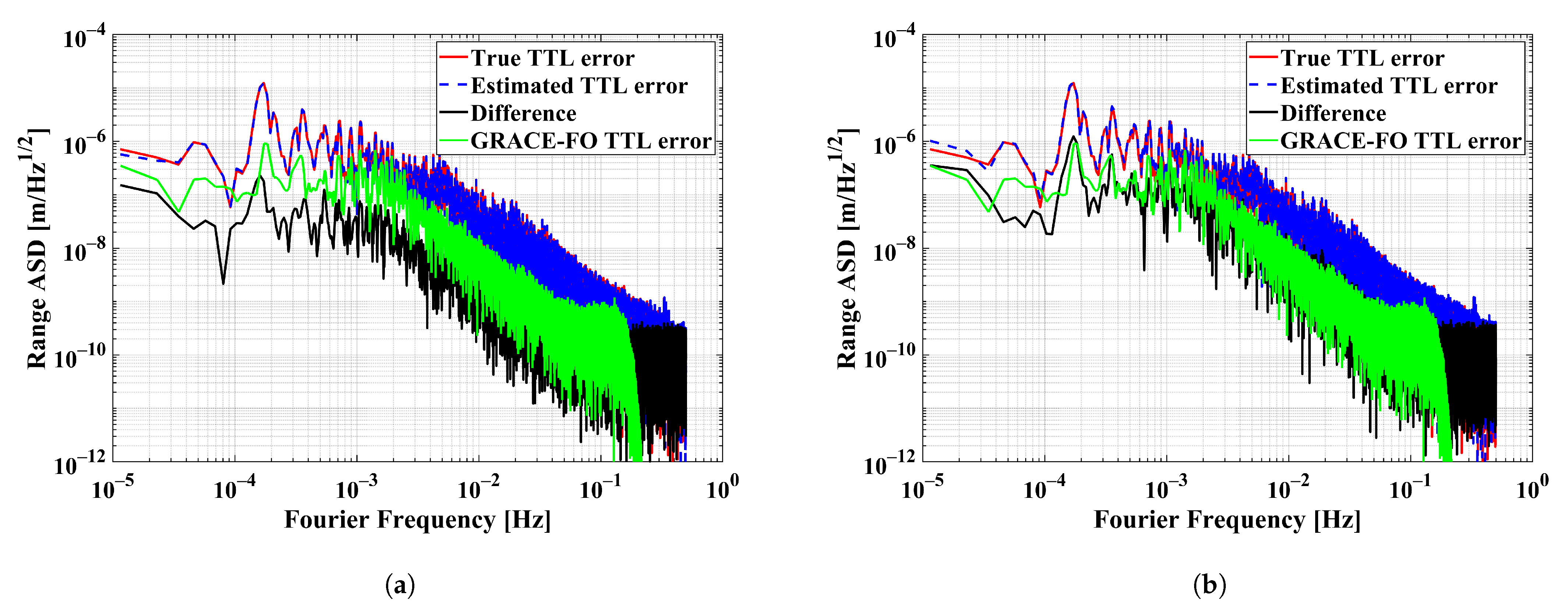
6.2. Results under L-Type Offset

6.2.1. Impact of Pointing Angle Noise

The same conditions as in Section 6.1.1 were applied, except that the offsets were set to Δ x = 1500 mm and Δ y = Δ z = 0.5 mm for each satellite. Four linear and two quadratic coupling factors { p x , 1 , p y , 1 , p z , 1 , p x , 2 , p y , 2 , p z , 2 } were estimated. Figure 11 shows the TTL estimation error and Table 6 shows the TTL coupling factors under different cases. Taking the angle biases into account, the large longitudinal offsets yield additional linear coupling terms according to Equation (29). These terms were absorbed by the linear coupling factors in the TTL estimation. The pitch and yaw angle biases { Δ θ y , 1 , Δ θ z , 1 , Δ θ y , 2 , Δ θ z , 2 } we used here are set to { 500 , 300 , 400 , 700 } μ rad . As a result, the quadratic coupling factors deviate from the input values (see Table 6) and the desired values of the linear coupling factors p y , i and p z , i ( i = 1 , 2 ) can be computed by the following equation:
p y , i = Δ θ z , i Δ x i Δ y i , p z , i = Δ θ y , i Δ x i + Δ z i .
Similarly to the results under the S-type offset, the pointing angle noise should be lower than 1 μ rad / Hz 1 / 2 to perform a successful TTL estimation.

6.2.2. Impact of Lateral Offset

Estimation results of different lateral offsets are shown in Figure 12 and Table 7, where the pointing angle noise level was set to 0.1 μ rad / Hz 1 / 2 and the angle biases we used are the same as in the previous subsection.
It can be seen in Figure 12 that the levels of estimation error (black) of the four cases are similar except at high frequencies, similar to the corresponding results under the S-type offset in Figure 9. Therefore, similar conclusion can be drawn that the lateral offset is not of great significance for TTL estimation even if the longitudinal offsets are large when the angle noise level is as low as 0.1 μ rad / Hz 1 / 2 .

6.2.3. Impact of Laser Frequency Noise

The impact of different laser frequency noise is shown in Figure 13 and Table 8. The angle biases and noise are the same as in the previous subsection and the offset vector was set to 1500 0.5 0.5 mm for each satellite.
Although higher laser frequency noise was added in case (b), the error of TTL estimation (black) does not exceed the TTL error of GRACE-FO (green) at the frequency band shown in Figure 13b. In other words, one can eliminate the TTL error with 1.5 m offsets to an equivalent low level caused by 0.5 mm offsets even if the frequency stability performance of the laser is an order of magnitude worse than GRACE-FO.

7. Discussion

In order to better compare the TTL estimation results under different conditions, the RMS values of the estimation error were computed after subtracting the mean since the constant term is meaningless for the biased range. The error of the TTL estimation is mainly contributed by the linear terms and can be written as
δ ρ err , TTL i = 1 2 δ θ y , i ( θ y , i p x , i + p z , i ) + δ θ z , i ( θ z , i p x , i + p y , i ) + θ z , i Δ p y , i + θ y , i Δ p z , i .
Here, Δ p k , i ( k = y , z ) denotes the difference between the estimated linear coupling factor p ^ k , i and the true value p k , i . The first two terms in Equation (54) are induced by the angle noise δ θ k , i , while the last two terms are due to the estimation error of the linear coupling factor Δ p k , i .
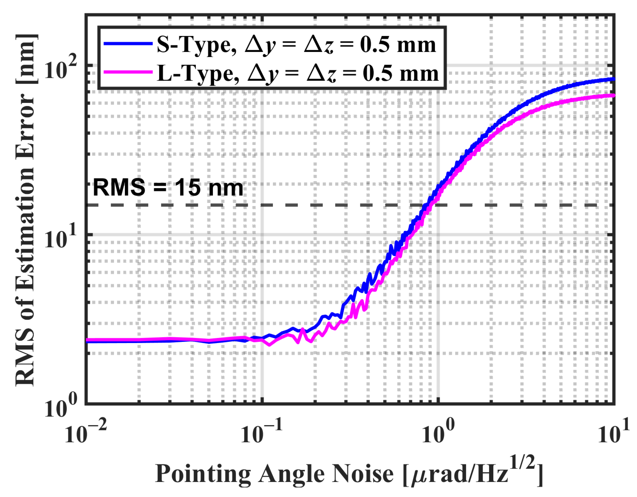
Figure 14 shows the RMS values of the estimation error under different pointing angle noise in the cases of S-type (blue) and L-type (magenta) longitudinal offsets. Figure 15 shows the RMS values of the estimation error under different lateral offsets and laser frequency noise in various cases. The dashed black lines in Figure 14 and Figure 15 represent the RMS level of GRACE-FO’s TTL error.
The two traces in Figure 14 are flat at angle noise below 0.3 μ rad / Hz 1 / 2 with the values lower than 4 nm probably because the ranging noise (mainly the laser frequency noise and the added noise introduced by the accelerometers) limits the TTL estimation, which yields similar estimation error for the coupling factors in the last two terms in Equation (54) under different angle noise. As the angle noise δ θ k , i increases, the first two terms grow proportionally and the coupling factor error Δ p k , i in the last two terms also increases, leading to the rising parts of the traces. As the RMS values of the estimation error reach the levels of the input TTL error, the two traces gradually show a trend to become flat. It can be seen in Figure 14 that to eliminate the TTL error to the level lower than the TTL error of GRACE-FO, the angle noise should be lower than 1 μ rad / Hz 1 / 2 , as mentioned above, or lower than 0.3 μ rad / Hz 1 / 2 for a better result. One can also see the obvious difference between the results with 0.1 μ rad / Hz 1 / 2 (blue and magenta) and 1 μ rad / Hz 1 / 2 angle noise (red and green) in Figure 15, so it is important to achieve low noise angle measurement for the estimation approach in this study.
The blue and magenta traces in Figure 15a are flat over a wide range of lateral offsets due to the limitation of the coupling factor error in the last two terms of Equation (54), while the flat part of the green trace is narrower, and the red trace shows no flat parts since it is dominated by the first two terms of Equation (54), which is proportional to the pointing angle noise and the lateral offset. The flat parts of the blue and magenta traces in Figure 15b are mainly limited by the coupling factor error, which is not induced by the laser frequency noise but other error sources, such as the accelerometer noise, while the red and green ones are limited by the pointing angle noise. As the lateral offsets grow, the slopes of the traces in Figure 15a (e.g., the red, blue, and magenta traces) will no longer be an approximate zero value since the first two terms, which are proportional to the lateral offsets, start to dominate the estimation error, while the coupling factor error in the last two terms does not vary a lot. In contrast, the rising parts of the traces in Figure 15b (e.g., the blue and magenta traces) are due to the increasing coupling factor error in the last two terms caused by the increasing laser ranging noise.
Figure 14 and Figure 15 do not show much difference between the results of S-type and L-type offsets except for the red and green traces in Figure 15a. The pointing angles used in TTL estimation contain biases of several hundreds of μ rad , inducing additional linear coupling terms in the case of the L-type offset. Since the input angle biases were different from each other, varying from zero to several hundreds of microns, even if the input lateral offsets were set to zeros, the coefficients of the additional linear coupling terms would behave like the lateral offsets and contribute to the coupling factors p y , i and p z , i in the first two terms of Equation (54), which is responsible for the flat part of the green trace. The additional linear terms in the case of the S-type offset can be omitted so the red trace behaves normally. In addition, the slope of the rising part of the green trace is slightly larger than 1, mainly due to the non-negligible terms θ y , i p x , i and θ z , i p x , i in Equation (54), where the coupling factor p x , i is up to 1.5 m / rad 2 . The influence of these two terms will be much smaller in the case of the S-type offset; thus, the slope of the rising part of the red trace is almost 1.
Assuming that the CM-VP lateral offset will not exceed 0.5 mm and the performance of the laser frequency stability will be the same as GRACE-FO, the main limitation for the investigated approach to TTL estimation is the pointing angle noise. One drawback of this research is that the input attitude data were obtained from the official SCA1B data of GRACE-FO, which may deviate the actual cases in future gravity missions. The actual pointing angles at the passband may be lower, mandating stronger restrictions on the accuracy of angle measurement. All in all, the pointing angle noise level is absolutely the key to successful TTL estimation in this study. However, the official LSM1B data product of GRACE-FO only provides angle measurement with a noise level of a few μ rad / Hz 1 / 2 , which is not precise enough for the estimation method in this paper. Therefore, attitude sensors with higher precision, such as an advanced position sensor system for the FSM based on the one in GRACE-FO or an interferometer readout system for FSM actuation angles, may be implemented in future gravity missions. The accelerometer noise model in this study plays a similar role as the laser frequency noise since the ACC noise enters when subtracting the differential non-gravitational range, and we found the contributions of the ACC noise and the laser frequency noise to the ranging data in the passband are at the similar level. Moreover, we expect better performance from the accelerometers in future gravimetry missions so that the ACC noise will not be a restriction, and thus, the impacts under different accelerometer noise are not discussed individually in this paper.
As the large TTL error induced by the L-type longitudinal offset can be subtracted to a low level, it is not necessary to install the VP of the TMA at the center of mass, which results in some flexibility to the installation layout of the satellite platform. For example, a smaller TMA in a redundant LRI may be installed 1.5 m far away from the center of mass just like the KBR case. Additionally, the estimation approach can be performed daily, making it possible to monitor the variations in the CM-VP offset day-by-day, which could provide daily and seasonal estimations for the CM movement [14].

8. Conclusions

Non-constant systematic TTL error is commonly seen in low-low satellite-to-satellite tracking missions like GRACE and GRACE-FO, and TTL estimation methods with certain calibration maneuvers have previously been investigated in both the KBR and LRI cases. In this paper, an alternative approach for LRI TTL estimation that overcomes the limitation of the time span of the calibration maneuvers has been presented. We introduced the basic working principle of LRI and derived two-way ranging formulations for LRI based on the dual one-way ranging formulations for KBR. The TTL model where the angle biases are taken into account was derived for parameter estimation, requiring data for satellite orbits, attitudes, and non-gravitational accelerations. Therefore, a numerical simulation was performed to generate the simulated GNI1B, SCA1B, ACC1B, LRI1B, and LSM1B data. Cases of S-type and L-type longitudinal offsets were discussed separately and no significant difference was found under low angle noise conditions between the two cases. By comparing the estimation results of the TTL error and the coupling factors, it was found that the impact of the pointing angle noise was more apparent than the impact of the lateral offset and the laser frequency noise. When the pointing angle noise is below 0.3 μ rad / Hz 1 / 2 , the RMS of the TTL correction error will be lower than 4 nm in the cases of both S-type and L-type offsets, which is better than the current TTL level of GRACE-FO.
For future gravity missions with LRI, it is possible to perform pointing angle measurements at higher precision with advanced attitude sensors and, thus, the approach for TTL estimation introduced in this paper may be implemented. Since the TTL estimation error is not limited by the longitudinal offset, a redundant TMA can be mounted far away from the center of mass and its size can be reduced. Moreover, the daily estimated results of the coupling factors may be used for estimation of the center of mass movement.

Author Contributions

Conceptualization, Z.W. and H.D.; methodology, Z.W.; software, Z.W.; validation, S.Y. and F.L.; formal analysis, Z.W., S.Y., F.J., and K.W.; investigation, Z.W.; resources, H.D.; data curation, Z.W.; writing—original draft preparation, Z.W.; writing—review and editing, H.D. and H.-C.Y.; visualization, Z.W.; supervision, H.D.; project administration, H.-C.Y.; funding acquisition, H.D. and H.-C.Y. All authors have read and agreed to the published version of the manuscript.

Funding

This research was funded by the National Key R&D Program of China (No. 2020YFC2200202 and No. 2022YFC2204001) and the National Natural Science Foundation of China (NSFC) (No. 12005310).

Data Availability Statement

The official GRACE-FO Level-1B data products can be found at ftp://isdcftp.gfz-potsdam.de/grace-fo/ (accessed on 12 August 2023). The data generated in this study are not publicly available due to [its use in an ongoing study by the authors] but can be made available from the corresponding author upon reasonable request.

Acknowledgments

The authors would like to thank the LRI team at the Albert Einstein Institute for providing the GRACE-FO LRI1B (v50–v52, v54–v55) data.

Conflicts of Interest

The authors declare no conflicts of interest.

Abbreviations

The following abbreviations are used in this manuscript:
ACC              Accelerometer
AEIAlbert Einstein Institute
AFAccelerometer frame
AOCAntenna offset correction
APCAntenna phase center
ASDAmplitude spectral density
BSBeam splitter
CMCenter of mass
CMCCenter-of-mass calibration
CNRCarrier-to-noise ratio
CPCompensation plate
DOWRDual one-way ranging
DPLLDigital phase-locked loop
DSACDeep Space Atomic Clock
DWSDifferential wavefront sensing
FPFabry–Pérot
FSMFast steering mirror
GFOGRACE Follow-On
GNSSGlobal Navigation Satellite System
GPSGlobal Positioning System
GRACEGravity Recovery And Climate Experiment
GRACE-FO    GRACE Follow-On
GRACE-IGRACE-ICARUS (International Cooperation for Animal Research Using Space)
ICRFInternational Celestial Reference Frame
IFInertial frame
IMUInertial measurement unit
IPUInstrument processing unit
KBRK-band ranging
LISALaser Interferometer Space Antenna
LL-SSTLow-low satellite-to-satellite tracking
LOLocal oscillator
LOSLine of sight
LOSFLine-of-sight frame
LPFLISA Pathfinder
LRILaser ranging interferometer
LSQLeast squares
LTCLight time correction
MWIMicrowave ranging instrument
NGGMNext Generation Gravity Mission
OBOptical bench
OBCOnboard computer
OPLLOptical phase-locked loop
PDHPound–Drever–Hall
POD              Precision orbit determination
PSDPower spectral density
RMSRoot mean square
RXReceived
SATSatellite
SCAStar camera assembly
SFSatellite frame
TCGGeocentric coordinate time
TMATriple mirror assembly
TOFTime-of-flight
TTTerrestrial time
TTLTilt-to-length
TWRTwo-way ranging
TXTransmitted
USOUltrastable oscillator
VPVertex point
VPC              Vertex point correction

References

  1. Tapley, B.D.; Bettadpur, S.; Watkins, M.; Reigber, C. The Gravity Recovery and Climate Experiment: Mission Overview and Early Results. Geophys. Res. Lett. 2004, 31, L09607. [Google Scholar] [CrossRef]
  2. Landerer, F.W.; Flechtner, F.M.; Save, H.; Webb, F.H.; Bandikova, T.; Bertiger, W.I.; Bettadpur, S.V.; Byun, S.H.; Dahle, C.; Dobslaw, H.; et al. Extending the Global Mass Change Data Record: GRACE Follow-On Instrument and Science Data Performance. Geophys. Res. Lett. 2020, 47, e2020GL088306. [Google Scholar] [CrossRef]
  3. Sheard, B.S.; Heinzel, G.; Danzmann, K.; Shaddock, D.A.; Klipstein, W.M.; Folkner, W.M. Intersatellite laser ranging instrument for the GRACE follow-on mission. J. Geod. 2012, 86, 1083–1095. [Google Scholar] [CrossRef]
  4. Kornfeld, R.P.; Arnold, B.W.; Gross, M.A.; Dahya, N.T.; Klipstein, W.M.; Gath, P.F.; Bettadpur, S. GRACE-FO: The Gravity Recovery and Climate Experiment Follow-On Mission. J. Spacecr. Rocket. 2019, 56, 931–951. [Google Scholar] [CrossRef]
  5. Chwalla, M.; Danzmann, K.; Fernández Barranco, G.; Fitzsimons, E.; Gerberding, O.; Heinzel, G.; Killow, C.J.; Lieser, M.; Perreur-Lloyd, M.; Robertson, D.I.; et al. Design and construction of an optical test bed for LISA imaging systems and tilt-to-length coupling. Class. Quantum Gravity 2016, 33, 245015. [Google Scholar] [CrossRef]
  6. Tröbs, M.; Schuster, S.; Lieser, M.; Zwetz, M.; Chwalla, M.; Danzmann, K.; Barránco, G.F.; Fitzsimons, E.D.; Gerberding, O.; Heinzel, G.; et al. Reducing tilt-to-length coupling for the LISA test mass interferometer. Class. Quantum Gravity 2018, 35, 105001. [Google Scholar] [CrossRef]
  7. Chwalla, M.; Danzmann, K.; Álvarez, M.D.; Delgado, J.J.E.; Fernández Barranco, G.; Fitzsimons, E.; Gerberding, O.; Heinzel, G.; Killow, C.J.; Lieser, M.; et al. Optical Suppression of Tilt-to-Length Coupling in the LISA Long-Arm Interferometer. Phys. Rev. Appl. 2020, 14, 014030. [Google Scholar] [CrossRef]
  8. Houba, N.; Delchambre, S.; Ziegler, T.; Hechenblaikner, G.; Fichter, W. LISA spacecraft maneuver design to estimate tilt-to-length noise during gravitational wave events. Phys. Rev. D 2022, 106, 022004. [Google Scholar] [CrossRef]
  9. Hartig, M.S.; Wanner, G. Tilt-to-length coupling in LISA Pathfinder: Analytical modelling. Phys. Rev. D 2023, 108, 022008. [Google Scholar] [CrossRef]
  10. Wegener, H. Analysis of Tilt-to-Length Coupling in the GRACE Follow-On Laser Ranging Interferometer. Ph.D. Thesis, Gottfried Wilhelm Leibniz Universität Hannover, Hannover, Germany, 2022. [Google Scholar]
  11. Wang, F. Study on Center of Mass Calibration and K-Brand Ranging System Calibration of the GRACE Mission. Ph.D. Thesis, The University of Texas at Austin, Austin, TX, USA, 2003. [Google Scholar]
  12. Case, K.; Kruizinga, G.; Wu, S. GRACE Level 1B Data Product User Handbook; JPL D-22027; Jet Propulsion Laboratory: Pasadena, CA, USA, 2010.
  13. Wen, H.Y.; Kruizinga, G.; Paik, M.; Landerer, F.; Bertiger, W.; Sakumura, C.; Bandikova, T.; Mccullough, C. Gravity Recovery and Climate Experiment Follow-On (GRACE-FO) Level-1 Data Product User Handbook; JPL D-56935; Jet Propulsion Laboratory: Pasadena, CA, USA, 2019.
  14. Wegener, H.; Müller, V.; Heinzel, G.; Misfeldt, M. Tilt-to-Length Coupling in the GRACE Follow-On Laser Ranging Interferometer. J. Spacecr. Rocket. 2020, 57, 1362–1372. [Google Scholar] [CrossRef]
  15. Horwath, M.; Lemoine, J.M.; Biancale, R.; Bourgogne, S. Improved GRACE science results after adjustment of geometric biases in the Level-1B K-band ranging data. J. Geod. 2011, 85, 23–38. [Google Scholar] [CrossRef]
  16. Nicklaus, K.; Cesare, S.; Massotti, L.; Bonino, L.; Mottini, S.; Pisani, M.; Silvestrin, P. Laser metrology concept consolidation for NGGM. CEAS Space J. 2020, 12, 313–330. [Google Scholar] [CrossRef]
  17. Massotti, L.; Siemes, C.; March, G.; Haagmans, R.; Silvestrin, P. Next Generation Gravity Mission Elements of the Mass Change and Geoscience International Constellation: From Orbit Selection to Instrument and Mission Design. Remote Sens. 2021, 13, 3935. [Google Scholar] [CrossRef]
  18. Flechtner, F.M. Realization of a Satellite Mission “GRACE-I” for parallel Observation of Changing Global Water Resources and Biodiversity. In Proceedings of the AGU Fall Meeting 2020 Abstracts, Online, 7–11 December 2020. [Google Scholar]
  19. Drever, R.W.; Hall, J.L.; Kowalski, F.V.; Hough, J.; Ford, G.M.; Munley, A.J.; Ward, H. Laser phase and frequency stabilization using an optical resonator. Appl. Phys. B 1983, 31, 97–105. [Google Scholar] [CrossRef]
  20. Abich, K.; Abramovici, A.; Amparan, B.; Baatzsch, A.; Okihiro, B.B.; Barr, D.C.; Bize, M.P.; Bogan, C.; Braxmaier, C.; Burke, M.J.; et al. In-Orbit Performance of the GRACE Follow-on Laser Ranging Interferometer. Phys. Rev. Lett. 2019, 123, 031101. [Google Scholar] [CrossRef] [PubMed]
  21. Misfeldt, M.; Müller, V.; Müller, L.; Wegener, H.; Heinzel, G. Scale Factor Determination for the GRACE Follow-On Laser Ranging Interferometer Including Thermal Coupling. Remote Sens. 2023, 15, 570. [Google Scholar] [CrossRef]
  22. Morrison, E.; Meers, B.J.; Robertson, D.I.; Ward, H. Automatic alignment of optical interferometers. Appl. Opt. 1994, 33, 5041–5049. [Google Scholar] [CrossRef] [PubMed]
  23. Kim, J. Simulation Study of a Low-Low Satellite-to-Satellite Tracking Mission. Ph.D. Thesis, The University of Texas at Austin, Austin, TX, USA, 2000. [Google Scholar]
  24. Wu, S.C.; Kruizinga, G.; Bertiger, W. Algorithm Theoretical Basis Document for GRACE Level-1B Data Processing V1.2; JPL D-27672; Jet Propulsion Laboratory: Pasadena, CA, USA, 2006.
  25. Yan, Y.; Müller, V.; Heinzel, G.; Zhong, M. Revisiting the light time correction in gravimetric missions like GRACE and GRACE follow-on. J. Geod. 2021, 95, 48. [Google Scholar] [CrossRef]
  26. AEI LRI1B Products. Available online: https://www.aei.mpg.de/grace-fo-ranging-datasets (accessed on 12 August 2023).
  27. Darbeheshti, N.; Wegener, H.; Müller, V.; Naeimi, M.; Heinzel, G.; Hewitson, M. Instrument data simulations for GRACE Follow-on: Observation and noise models. Earth Syst. Sci. Data 2017, 9, 833–848. [Google Scholar] [CrossRef]
  28. Goswami, S.; Francis, S.P.; Bandikova, T.; Spero, R.E. Analysis of GRACE Follow-On Laser Ranging Interferometer Derived Inter-Satellite Pointing Angles. IEEE Sens. J. 2021, 21, 19209–19221. [Google Scholar] [CrossRef]
  29. Shinozuka, M.; Jan, C.M. Digital simulation of random processes and its applications. J. Sound Vib. 1972, 25, 111–128. [Google Scholar] [CrossRef]
  30. Thomas, J. An Analysis of Gravity-Field Estimation Based on Intersatellite Dual-1-Way Biased Ranging; JPL Publication 98-15; Jet Propulsion Laboratory: Pasadena, CA, USA, 1999.
  31. Larson, K.M.; Ashby, N.; Hackman, C.; Bertiger, W. An assessment of relativistic effects for low Earth orbiters: The GRACE satellites. Metrologia 2007, 44, 484–490. [Google Scholar] [CrossRef]
  32. Müller, V.; Hauk, M.; Misfeldt, M.; Müller, L.; Wegener, H.; Yan, Y.; Heinzel, G. Comparing GRACE-FO KBR and LRI Ranging Data with Focus on Carrier Frequency Variations. Remote Sens. 2022, 14, 4335. [Google Scholar] [CrossRef]
  33. Burt, E.A.; Prestage, J.D.; Tjoelker, R.L.; Enzer, D.G.; Kuang, D.; Murphy, D.W.; Robison, D.E.; Seubert, J.M.; Wang, R.T.; Ely, T.A. Demonstration of a trapped-ion atomic clock in space. Nature 2021, 595, 43–47. [Google Scholar] [CrossRef]
Figure 1. Overview of LRI optical components. The master satellite is named SAT1 and the transponder satellite is named SAT2. Each satellite includes at least a laser, a cavity, a fast steering mirror (FSM), a beam splitter (BS), a compensation plate (CP), and a triple mirror assembly (TMA). The vertex point (VP), an intersection point of three mirror planes of the TMA for each satellite, is nominally located at the center of mass (CM) of the satellite in the case of GRACE-FO.
Remotesensing 16 00862 g001
Figure 2. Phase observables of the two-way ranging system at actual time and their combinations. Detailed descriptions are in the main text.
Remotesensing 16 00862 g002
Figure 3. Geometric relationship of reference points and reference frames. The dashed line between C M 1 and C M 2 is called the line of sight (LOS) and e LOS , i is the unit vector pointing from one C M i ( i = 1 , 2 ) to the other one. V i is the vector pointing from C M i to V P i . The point P i is on the LOS and the line segment between C M i and P i is the projection of V i . The origin of the satellite frame (SF) and the line-of-sight frame (LOSF) is the C M of the corresponding satellite. For each satellite, the x-axis of LOSF coincides with the LOS, while the x-axis of the SF is slightly misaligned with the LOS due to the variability of satellite attitudes and the z-axes of both frames are roughly in the nadir direction.
Remotesensing 16 00862 g003
Figure 4. LRI ranging signal (blue), typical TTL error (magenta and green), and error contributed by laser frequency variations (red) in terms of ASD. Official GRACE-FO LRI1B v04 (version 04, or called RL04) data product on 1 April 2021 is used to plot the blue trace. TTL error can be computed from Equation (27) as long as the CM-VP offset and pointing angles of each satellite are provided. The magenta trace is plotted using the official SCA1B v04 data on 1 April 2021, assuming a large CM-VP offset for each satellite, which is similar to the CM-APC offset in the GRACE mission. The GRACE-FO’s TTL error (green) of the same day is provided in the LRI1B v54 generated by AEI [26]. The red trace shows relativistic effects at several integer multiples of orbital frequency ( f orb 0.176 mHz ) and the error induced by random laser frequency noise which is generated according to Equation (1).
Remotesensing 16 00862 g004
Figure 5. Flowchart of the data simulation process. Data in the yellow boxes were obtained from the GRACE-FO RL04 Level-1B data products. We generated the error-free data based on the input and then added some error to obtain the simulated Level-1B data.
Remotesensing 16 00862 g005
Figure 6. Simulated instantaneous range and noise contributors in terms of ASD.
Remotesensing 16 00862 g006
Figure 7. Flowchart of the TTL estimation process.
Remotesensing 16 00862 g007
Figure 8. Input (red) and estimated (dashed blue) TTL error as well as their difference (black) under different pointing angle noise (the same noise level was applied to all pointing angles of the two satellites in each case). The TTL error of GRACE-FO on 1 April 2021 (green) was estimated by AEI [26]. (a) 0.01 μ rad / Hz 1 / 2 ; (b) 0.1 μ rad / Hz 1 / 2 ; (c) 1 μ rad / Hz 1 / 2 ; (d) 10 μ rad / Hz 1 / 2 .
Remotesensing 16 00862 g008
Figure 9. Input and estimated TTL error as well as their difference under different lateral offsets (the same value was applied to both Δ y and Δ z of the two satellites in each case). (a) 0.1 mm; (b) 0.5 mm; (c) 2.0 mm; (d) 5.0 mm.
Remotesensing 16 00862 g009
Figure 10. Input and estimated TTL error as well as their difference under different laser frequency noise (the ASD model in Equation (1) was multiplied by a factor to generate the laser frequency noise model in each case.) (a) 1 × ASD [ δ f cav ] ( f ) ; (b) 10 × ASD [ δ f cav ] ( f ) .
Remotesensing 16 00862 g010
Figure 11. Input and estimated TTL error as well as their difference under different pointing angle noise. (a) 0.01 μ rad / Hz 1 / 2 ; (b) 0.1 μ rad / Hz 1 / 2 ; (c) 1 μ rad / Hz 1 / 2 ; (d) 10 μ rad / Hz 1 / 2 .
Remotesensing 16 00862 g011
Figure 12. Input and estimated TTL error as well as their difference under different lateral offsets. (a) 0.1 mm; (b) 0.5 mm; (c) 2.0 mm; (d) 5.0 mm.
Remotesensing 16 00862 g012
Figure 13. Input and estimated TTL error as well as their difference under different laser frequency noise. (a) 1 × ASD [ δ f cav ] ( f ) ; (b) 10 × ASD [ δ f cav ] ( f ) .
Remotesensing 16 00862 g013
Figure 14. RMS values of estimation error under different pointing angle noise.
Remotesensing 16 00862 g014
Figure 15. RMS values of estimation error under different lateral offsets (a) and laser frequency noise in terms of multiples of the ASD model in Equation (1) (b).
Remotesensing 16 00862 g015
Table 1. Initial orbital elements of the two satellites.
Orbital ElementSAT1SAT2
Semi-major Axis6862.266 km6862.709 km
Eccentricity0.0009610.000907
Inclination89.088°89.088°
Argument of Periapsis79.795°77.920°
Longitude of the Ascending Node98.494°98.497°
True Anomaly163.952°164.201°
Table 2. Force models for orbit integration in the forward procedure and the POD procedure.
ParameterModel in Forward ProcedureModel in POD Procedure
Static Gravity FieldEIGEN-6C4 ( 180 × 180 )GGM05C ( 180 × 180 )
Solid Earth TidesIERS Conventions (2010)IERS Conventions (2010)
Ocean TidesFES2014b ( 180 × 180 )EOT11a ( 120 × 120 )
Solid Earth Pole TidesIERS Conventions (2010)IERS Conventions (2010)
Ocean Pole TidesDesai (2002) ( 180 × 180 )Desai (2002) ( 60 × 60 )
Atmosphere & Oceanic VariabilityAOD1B RL06 ( 180 × 180 )Not Considered
N-Body PerturbationsJPL DE440JPL DE440
Non-Gravitational ForcesACT1A & SCA1B RL04Simulated ACC1B & SCA1B
General Relativistic PerturbationsIERS Conventions (2010)IERS Conventions (2010)
Table 3. Input and estimated TTL coupling factors under different pointing angle noise.
Pointing Angle Noise
( θ y , 1 , θ y , 2 , θ z , 1 , θ z , 2 )
Coupling Factor
p y , 1 ( μ m / rad ) p z , 1 ( μ m / rad ) p y , 2 ( μ m / rad ) p z , 2 ( μ m / rad )
(a) 0.01 μ rad / Hz 1 / 2 487.7 ± 1.8 502.9 ± 2.7 508.8 ± 1.9 489.1 ± 3.0
(b) 0.1 μ rad / Hz 1 / 2 487.6 ± 1.9 500.9 ± 2.7 509.2 ± 1.9 487.6 ± 3.0
(c) 1 μ rad / Hz 1 / 2 420.1 ± 2.1 366.9 ± 2.8 451.2 ± 2.1 340.9 ± 3.0
(d) 10 μ rad / Hz 1 / 2 30.5 ± 0.8 18.1 ± 0.8 34.0 ± 0.8 15.4 ± 0.8
Input Value 500.0 500.0 500.0 500.0
Table 4. Estimated TTL coupling factors under different lateral offsets (S-Type offsets).
Lateral Offset
( Δ y 1 , Δ z 1 , Δ y 2 , Δ z 2 )
Coupling Factor
p y , 1 ( μ m / rad ) p z , 1 ( μ m / rad ) p y , 2 ( μ m / rad ) p z , 2 ( μ m / rad )
(a) 100 μ m 87.7 ± 1.8 102.1 ± 2.7 108.5 ± 1.9 89.6 ± 3.0
(b) 500 μ m 487.6 ± 1.9 500.9 ± 2.7 509.2 ± 1.9 487.6 ± 3.0
(c) 2000 μ m 1986.9 ± 1.9 1994.9 ± 2.9 2007.8 ± 2.0 1978.2 ± 3.2
(d) 5000 μ m 4988.4 ± 2.3 4976.3 ± 3.4 5008.7 ± 2.3 4962.4 ± 3.8
Table 5. Input and estimated TTL coupling factors under different laser frequency noise.
Laser Frequency Noise
(ASD Model)
Coupling Factor
p y , 1 ( μ m / rad ) p z , 1 ( μ m / rad ) p y , 2 ( μ m / rad ) p z , 2 ( μ m / rad )
(a) 1 × ASD [ δ f cav ] ( f ) 487.6 ± 1.9 500.9 ± 2.7 509.2 ± 1.9 487.6 ± 3.0
(b) 10 × ASD [ δ f cav ] ( f ) 550.1 ± 14.8 556.3 ± 21.9 499.7 ± 14.9 551.9 ± 24.2
Input Value 500.0 500.0 500.0 500.0
Table 6. Input, desired, and estimated TTL coupling factors under different pointing angle noise. The desired values are computed based on Equation (29) considering the angle biases.
Pointing Angle Noise
( θ y , 1 , θ y , 2 , θ z , 1 , θ z , 2 )
Coupling Factor
p x , 1 ( mm / rad 2 ) p y , 1 ( μ m / rad ) p z , 1 ( μ m / rad ) p x , 2 ( mm / rad 2 ) p y , 2 ( μ m / rad ) p z , 2 ( μ m / rad )
(a) 0.01 μ rad / Hz 1 / 2 1474.9 ± 14.7 34.7 ± 2.7 227.5 ± 14.6 1598.0 ± 12.7 1654.3 ± 12.8 1163.6 ± 9.6
(b) 0.1 μ rad / Hz 1 / 2 1474.7 ± 14.8 33.7 ± 2.7 232.4 ± 14.7 1597.3 ± 12.8 1654.1 ± 12.9 1162.8 ± 9.7
(c) 1 μ rad / Hz 1 / 2 1255.9 ± 18.1 37.7 ± 3.3 349.7 ± 18.0 1343.5 ± 15.1 1406.9 ± 15.3 987.6 ± 11.4
(d) 10 μ rad / Hz 1 / 2 83.2 ± 7.3 4.0 ± 1.2 48.8 ± 7.2 37.2 ± 5.4 42.7 ± 5.5 30.5 ± 4.0
Input Value1500-5005001500-500500
Desired Value1500-50-2501500-15501100
Table 7. Estimated TTL coupling factors under different lateral offsets (L-Type offsets).
Lateral Offset
( Δ y 1 , Δ z 1 , Δ y 2 , Δ z 2 )
Coupling Factor
p x , 1 ( mm / rad 2 ) p y , 1 ( μ m / rad ) p z , 1 ( μ m / rad ) p x , 2 ( mm / rad 2 ) p y , 2 ( μ m / rad ) p z , 2 ( μ m / rad )
(a) 100 μ m 1475.1 ± 14.8 365.7 ± 2.7 630.2 ± 14.7 1600.1 ± 12.7 1257.3 ± 12.9 768.3 ± 9.7
(b) 500 μ m 1474.7 ± 14.8 33.7 ± 2.7 232.4 ± 14.7 1597.3 ± 12.8 1654.1 ± 12.9 1162.8 ± 9.7
(c) 2000 μ m 1467.2 ± 15.3 1532.1 ± 2.8 1271.4 ± 15.2 1580.5 ± 13.2 3134.4 ± 13.3 2646.1 ± 10.0
(d) 5000 μ m 1447.4 ± 18.4 4532.7 ± 3.3 4281.0 ± 18.3 1638.7 ± 15.9 6186.3 ± 16.0 5669.5 ± 12.0
Table 8. Input, desired, and estimated TTL coupling factors under different laser frequency noise.
Laser Frequency Noise
(ASD Model)
Coupling Factor
p x , 1 ( mm / rad 2 ) p y , 1 ( μ m / rad ) p z , 1 ( μ m / rad ) p x , 2 ( mm / rad 2 ) p y , 2 ( μ m / rad ) p z , 2 ( μ m / rad )
(a) 1 × ASD [ δ f cav ] ( f ) 1474.7 ± 14.8 33.7 ± 2.7 232.4 ± 14.7 1597.3 ± 12.8 1654.1 ± 12.9 1162.8 ± 9.7
(b) 10 × ASD [ δ f cav ] ( f ) 1270.8 ± 118.6 134.2 ± 21.5 22.9 ± 117.7 1902.4 ± 102.3 1949.5 ± 103.2 1455.0 ± 77.5
Input Value1500–5005001500–500500
Desired Value1500–50–2501500–15501100
Disclaimer/Publisher’s Note: The statements, opinions and data contained in all publications are solely those of the individual author(s) and contributor(s) and not of MDPI and/or the editor(s). MDPI and/or the editor(s) disclaim responsibility for any injury to people or property resulting from any ideas, methods, instructions or products referred to in the content.

