Physics-Based Satellite-Derived Bathymetry (SDB) Using Landsat OLI Images

Abstract

The estimation of depth in optically shallow waters using satellite imagery can be efficient and cost-effective. Active sensors measure the distance traveled by an emitted laser pulse propagating through the water with high precision and accuracy if the bottom peak intensity of the waveform is greater than the noise level. However, passive optical imaging of optically shallow water involves measuring the radiance after the sunlight undergoes downward attenuation on the way to the sea floor, and the reflected light is then attenuated while moving back upward to the water surface. The difficulty of satellite-derived bathymetry (SDB) arises from the fact that the measured radiance is a result of a complex association of physical elements, mainly the optical properties of the water, bottom reflectance, and depth. In this research, we attempt to apply physics-based algorithms to solve this complex problem as accurately as possible to overcome the limitation of having only a few known values from a multispectral sensor. Major analysis components are atmospheric correction, the estimation of water optical properties from optically deep water, and the optimization of bottom reflectance as well as the water depth. Specular reflection of the sky radiance from the water surface is modeled in addition to the typical atmospheric correction. The physical modeling of optically dominant components such as dissolved organic matter, phytoplankton, and suspended particulates allows the inversion of water attenuation coefficients from optically deep pixels. The atmospheric correction and water attenuation results are used in the ocean optical reflectance equation to solve for the bottom reflectance and water depth. At each stage of the solution, physics-based models and a physically valid, constrained Levenberg–Marquardt numerical optimization technique are used. The physics-based algorithm is applied to Landsat Operational Land Imager (OLI) imagery over the shallow coastal zone of Guam, Key West, and Puerto Rico. The SDB depths are compared to airborne lidar depths, and the root mean squared error (RMSE) is mostly less than 2 m over water as deep as 30 m. As the initial choice of bottom reflectance is critical, along with the bottom reflectance library, we describe a pure bottom unmixing method based on eigenvector analysis to estimate unknown site-specific bottom reflectance.

1. Introduction

Accurate, quantitative measurements of nearshore bathymetry (water depths 0–30 m) are important for the assessment of hazards to and management of coastal communities, infrastructure, agriculture, and ecosystems associated with storm events and sea-level rise. Measurements of coastal waters are typically acquired by active sensors such as lidar or sonar. Bathymetric lidar uses a green laser pulse because this wavelength has minimal attenuation by coastal water in most cases. The operating depth range of bathymetric lidar is mainly determined by the attenuation coefficient: a high-powered, state-of-the-art bathymetric lidar can pick up a return pulse from a sea floor as deep as 70 m when the water is very clear, with a diffuse attenuation coefficient around 0.6 m⁻¹ at 532 nm. However, in most cases, a bathymetric lidar can detect bottom return peaks only over much shallower regions.

The passive optical technique for mapping bathymetry can use airborne images or satellite images. The main drawback of lidar or sonar is the relatively high cost. In contrast, many no-cost globally available nearshore satellite images are available and make satellite-derived bathymetry (SDB) an attractive alternative. Typically, airborne data require mosaicking data from flight lines or stitching thousands of individual images. Although airborne images can have very small pixels, a common drawback is radiometric imbalance between scanlines or frames due to variations in roll, pitch, and heading angle. When the sun is in the cross-track direction, this imbalance is worse than when the sun is closer to the along-track direction. However, satellite images are virtually free of the radiometric imbalance issue because the satellite sensor orientation is invariant during the overpass.

Since Lyzenga suggested an SDB method [1,2], Stumpf et al. developed an SDB method for high-resolution satellite imagery [3], and there are many SDB variants and other types of coastal bathymetric techniques [4]. We propose a physics-based SDB technique for any multispectral satellite sensor that has 3–5 bands in the visible spectral range. This is the most prevalent satellite sensor type and includes the Landsat Operational Land Imager (OLI), the Sentinel-2 MultiSpectral Instrument (MSI), and the WorldView series. In this research, we use Landsat OLI data, which are freely available from U.S. Geological Survey (USGS) public data access points, such as USGS EarthExplorer [5], USGS GloVis [6], and LandsatLook Viewer [7].

2. Methods

This section comprehensively explores the concepts, theories, and algorithms of physics-based SDB. Special emphasis is placed on the technique to guarantee that the nonlinear optimization algorithm we use converges to physically valid solutions.

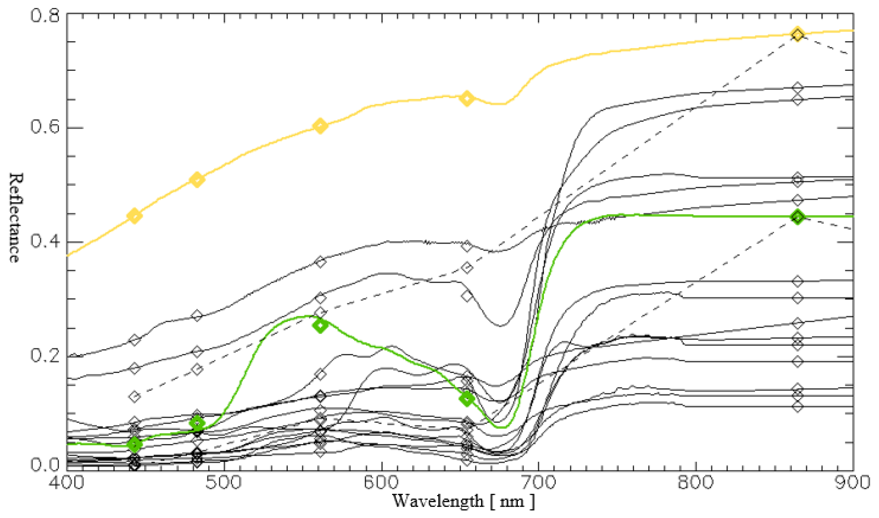
2.1. Sampling Optically Deep Water Pixels

By definition, pixels from an area of optically deep water are free from bottom influence. The optical depth of the water is calculated by multiplying the geometrical depth and the attenuation coefficient and is thus dimensionless. Beyond a certain optical depth (for instance, 3.0), the bottom reflected signal is almost completely attenuated; thus, it is called “optically deep”. In optically deep water, the radiance is determined by the inherent optical properties (IOPs) of the water and the atmospheric contribution. After atmospheric correction, only the effect of the optical properties remains, and one can solve for the IOPs using the ocean optical model presented in Section 2.4.2. Therefore, the first step of physics-based SDB is sampling a pixel spectrum from optically deep water. The current method requires the existence of optically deep water in the scene. The top-of-the-atmosphere (TOA) reflectance is obtained as an irradiance ratio based on the Lambertian assumption. After correction by solar zenith angle and earth–sun distance, it is given by the following equation:

$${\rho }_{TOA}=\frac{\pi ·L_{TOA}·D_{ES}^2}{\mathrm{c}\mathrm{o}\mathrm{s}SZA·F_0}$$

(1)

The description of the variables is found in

Table 1. List of variables.

Variable	Name	Unit
${\rho }_{TOA}$	Top of the atmosphere (TOA) reflectance	Unitless
$L_{TOA}$	TOA radiance	[W m−2 nm−1 sr−1]
$D_{ES}$	Earth to Sun distance	AU
$SZA$	Solar zenith angle	Radian
$F_0$	Exoatmospheric solar irradiance	[W m−2 nm−1]
$VZA$	View zenith angle	Radian
${\tau }_a$	Aerosol optical depth at 550 nm	Unitless
$U_{oz}$	Column ozone	[DU]
$U_{wv}$	Column water vapor	[cm]
$P$	Surface pressure	Millibars
${\rho }_{atm+sfc}$	Atmospheric and water surface reflectance	Unitless
$A_s$	Atmospheric spherical albedo	Unitless
$T_{og}$	Transmission by absorption of other gases	Unitless
$T_{oz}$	Transmission by absorption of ozone	Unitless
$T_{wv}$	Transmission by absorption of water vapor	Unitless
$t_s$	Transmission by scattering (sun to surface)	Unitless
$t_v$	Transmission by scattering (surface to sensor)	Unitless
${\rho }_{BOA}$	Bottom of the atmosphere (BOA) reflectance	Unitless
$R_{rs}$	Above-water remote sensing reflectance	[sr−1]
$r_{rs}$	Subsurface remote sensing reflectance	[sr−1]
$g_1, g_2$	Coefficients of quadratic IOP’s model for $r_{rs,\infty }$	Unitless
$u$	Backward scattering to total forward attenuation	Unitless
$a$	Total absorption coefficient	[m−1]
$b_b$	Total backward scattering coefficient	[m−1]
$a_w$	Absorption coefficient due to pure water	[m−1]
$a_{dg}$	Absorption coefficient due to detritus and gelbstoff	[m−1]
$S$	Exponential coefficient of $a_{dg}$ function	[nm−1]
$a_{ph}$	Absorption coefficient due to phytoplankton	[m−1]
$C$	Chlorophyll-a concentration	[mg m3]
${a_C}^{*}$	Normalized absorption by average phytoplankton	[m−1]
$b_w$	Backward scattering due to pure water	[m−1]
$b_{bp}$	Scattering coefficient due to suspended particulate	[m−1]
$n$	Power coefficient of $b_{bp}$ function	Unitless
$e$	Difference between measured and modeled	N/A
$X$	Physical parameter $X$	N/A
$\Phi$	Generic parameter for bounded solution of $X$	N/A
$\mathit{J}$	Jacobian for derivative-based optimization	N/A
$K_d$	Downward diffuse attenuation coefficient	[m−1]
$K_u$	Upward diffuse attenuation coefficient	[m−1]
$SZA\_w$	In-water refracted solar zenith angle (SZA)	[radian]
$VZA\_w$	In-water refracted view zenith angle (VZA)	[radian]
$n_w$	Refractive index of coastal water	Unitless
$r_{rs,\infty }$	$r_{rs}$ from optically deep water	[sr−1]
$z$	Geometrical depth of optically shallow water	[m]
${\rho }_b$	Bottom albedo	Unitless
$C_s, C_g$	Proportion of sand-like and grass-like bottom	Unitless
${\rho }_{bs}, {\rho }_{bg}$	Bottom albedo of sand-like and grass-like bottom	Unitless
$\mathit{w}$	Weight vector for all bands, $w\left({\lambda }_i\right) :i=1,\dots ,N_w$	Unitless
$N_w$	Number of wave bands	Unitless

. The Landsat OLI level-1 precision and terrain correction image product (L1TP) provides ${\rho }_{TOA}·\mathrm{c}\mathrm{o}\mathrm{s}SZA$, which is the TOA reflectance without solar zenith angle (SZA) correction. Thus, the OLI L1TP image needs to be divided by the cosine of the accompanied SZA image before atmospheric correction. The radiance, irradiance, and reflectance are a function of wavelength. However, wavelength dependency will be suppressed in most cases to make the notation more compact.

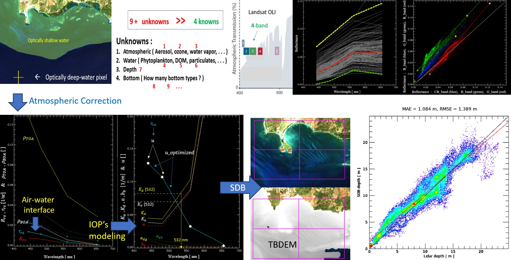
2.2. Atmospheric Correction

The water-leaving radiance is modified by the presence of air molecules and aerosols detected by the sensor as TOA radiance. Roughly speaking, a majority (about 80% or more) of the at-sensor radiance is due to atmospheric scattering, which needs to be removed to apply the SDB technique. Because the radiance originating from the water body is relatively small, minor errors in atmospheric correction will result in larger errors in the estimated depth, making accurate atmospheric correction critical. A commonly used and well-established method based on atmospheric radiative transfer modeling is used in this research. Look-up-tables (LUTs) of the pre-computed atmospheric radiative transfer solution, such as MODTRAN [8,9] or 6SV [10,11], are commonly used for atmospheric correction.

In addition to the generic LUT approach, a specific emphasis in this SDB research is the effect of the water surface. The radiance from the water surface, unlike the terrestrial surface, has an additional contribution from the reflected sky radiance. Taking this component into account is important for accurately estimating depth via the SDB method.

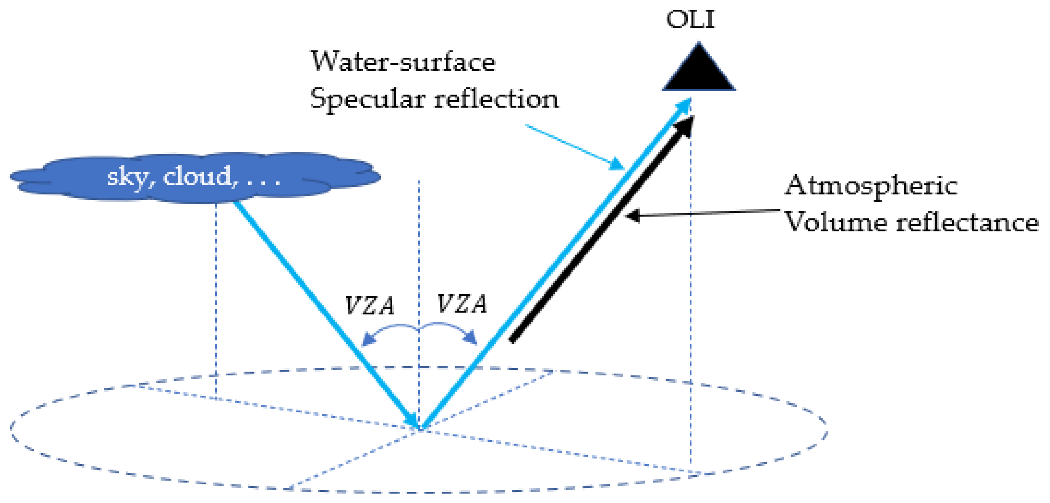
2.2.1. Atmospheric Radiative Transfer over Coastal Zone

The sky area that gives extra radiance to a pixel due to specular reflection at the water surface is determined by several factors. A specular reflection of a sky to the image occurs on a three-dimensional plane that includes the view direction vector and the surface normal vector (Figure 1).

Although the Ahmad LUT [12] provides background reflected sky reflectance, the nature of the sky area is not known due to the complex and random nature of the sky. For example, if a puffy white cloud is present, then the downward sky radiance will be high, which requires more correction than the Ahmad LUT would estimate. If the cloud is dark, the downward sky radiance will be lower than for a typical cloud-free blue background sky. Thus, once the background reflected sky reflectance is applied, a subsequent dark-pixel algorithm needs to be applied to fix the pixel-by-pixel variation of the sky condition [13,14].

2.2.2. Aerosol Optical Depth Inversion Based on Dark Water Concept

Because OLI lacks the bands to estimate pressure, column ozone, and column water vapor, constant values are used in creating the LUT. Only red and green bands are affected by ozone, and the effect of varying ozone amount is not substantial; a global average of 300 DU $U_{oz}$ is used in LUT generation. OLI bands are chosen to avoid water vapor absorption. Although any value should work, a typical value of 3 cm $U_{wv}$ is used in LUT generation. Because SDB applies to the coastal zone near the mean sea level, the pressure value of 1013 mb is used in LUT generation. A “coastal” aerosol type is the most appropriate for SDB. As the effect of the atmospheric model is minimal, a “mid-latitude summer” model is used. The ${\rho }_{atm+sfc}$ LUT is generated by varying ${\tau }_a$ along with all feasible angular combinations of SZA, view zenith angle (VZA), and relative azimuth angles, where the angle notations are dropped for a simpler notation as follows: $\left({\tau }_a;U_{oz},U_{wv},P\right)\to LUT: {\rho }_{atm+sfc}(\lambda ;{\tau }_a)$.

The major component of the LUT is ${\rho }_{atm}$, but it also creates auxiliary tables for atmospheric scattering transmittances for downward $t_s$ and upward $t_v$; atmospheric spherical albedo $A_s$; and molecular gas transmittance $T_{og},T_{oz}, T_{wv}$ for other gases, ozone, and water vapor, respectively. The primary goal of atmospheric correction is to determine ${\tau }_a$ based on a dark water concept, which makes ${\rho }_{TOA}\left({\lambda }_{NIR}\right)$ zero after correction. Thus, the atmospheric correction involves finding ${\tau }_a$ that satisfies ${\rho }_{atm+sfc}\left({\lambda }_{NIR};{\tau }_a\right)={\rho }_{TOA}\left({\lambda }_{NIR}\right)$.

Once the optimized solution of ${\tau }_a$ is obtained, the following formula solves for the surface reflectance at the bottom of the atmosphere:

$${\rho }_{BOA}=\frac{{\rho }_s^{\prime }}{1+A_s\cdot {\rho }_s^{\prime }},{\rho }_s^{\prime }=\frac{{\rho }_{TOA}-{\rho }_{atm+sfc}\left({\tau }_a\right)}{T_{og}\cdot T_{oz}\cdot T_{wv}\cdot t_s\left({\tau }_a\right)\cdot t_v\left({\tau }_a\right)}$$

(2)

2.3. Conversion to Subsurface Remote Sensing Reflectance

The above-surface, remote-sensing reflectance $R_{rs}$ is obtained from surface reflectance divided by $\pi$ based on the Lambertian radiance distribution assumption. The conversion of subsurface remote sensing reflectance $r_{rs}$ from the above surface remote sensing reflectance $R_{rs}$ is derived from the following formula [15]:

$$r_{rs}=\frac{R_{rs}}{0.52+1.7R_{rs}},R_{rs}=\frac{{\rho }_{BOA}}{\pi }$$

(3)

Equation (3) is valid for VZAs around 20° or smaller. For a greater view angle, a different ocean optical radiative transfer simulation and modeling is needed to determine a proper set of coefficients in Equation (3). However, most satellites collect imagery within a narrow range of angles around the nadir. For Landsat OLI imagery, for example, the maximum VZA is 7.5°, which is well within the range of validity for Equation (3).

2.4. Ocean Optical Inversion of Inherent Optical Properties

2.4.1. Subsurface Reflectance Model of IOPs

The optically deep subsurface remote sensing reflectance $r_{rs,\infty }$ is modeled as a quadratic function of an IOP’s model quantity $u$, which is the ratio of backward scattering to total forward beam attenuation [16]:

$$r_{rs,\infty }=g_1·u+g_2·u^2,g_1=0.0949,g_2=0.0794, u\equiv \frac{b_b}{a+b_b}.$$

(4)

The backward scattering determines the number of photons that are scattered backward by water molecules and other particulates and that travel back through the air and eventually to the sensor. The total forward attenuation determines how many photons are removed from the photon pool that is potentially available for backward scattering. Thus, the ratio of backward scattering to forward beam attenuation is related to the remote sensing radiance. The more backward scattering, the higher the remote sensing radiance. The higher the forward beam attenuation, the lower the remote sensing radiance. This ratio is related to the subsurface remote sensing reflectance in a quadratic manner. This relationship is derived using the simulated radiance for given IOPs by running an ocean optical radiative transfer model, such as Hydrolight [17].

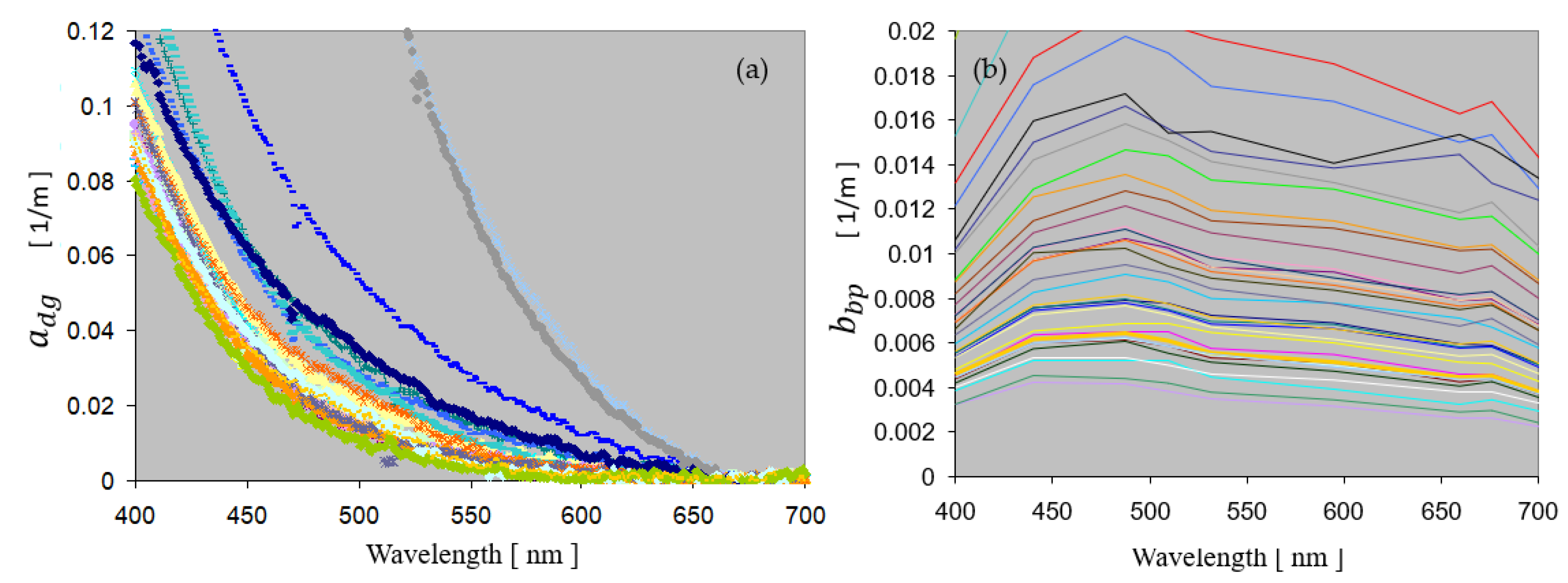
2.4.2. Ocean Optical Models of Inherent Optical Properties

The absorption model for detritus and gelbstoff (also called carbonaceous dissolved organic matter) is given by

$$a_{dg}\left(\lambda \right)=a_{dg}\left({\lambda }_0\right)·\mathrm{e}\mathrm{x}\mathrm{p}[-S·\left(\lambda -{\lambda }_0\right)],$$

(5)

where $S$ is the coefficient that describes exponentially decreasing absorption with wavelength, and ${\lambda }_0$ is a reference wavelength with a typical value of 440 nm. Example $a_{dg}$ spectra, which were measured via in situ ground truth optical data collection from various locations with different optical conditions during the Coastal Zone Mapping and Imaging Lidar (CZMIL) validation campaign at Thunder Bay, Alpena, Michigan, USA, in 2007 [18], are presented in Figure 2. They show an excellent match with the analytical exponential model.

$$a_{ph}\left(\lambda \right)=0.06·C^{0.65}·{a_C}^{*}\left(\lambda \right),$$

(6)

where $C$ is the chlorophyll-a concentration in [mg/m³], and ${a_C}^{*}$ is the normalized spectral absorption by the phytoplankton in global average. The total absorption combines water absorption $a_w$ and the two components.

$$a\left(\lambda \right)=a_w\left(\lambda \right)+a_{dg}\left(\lambda \right)+a_{ph}\left(\lambda \right)$$

(7)

Backward scattering due to suspended particulates was also measured along with $a_{dg}$ spectra (Figure 2b), and it is modeled as a power function with a typical reference wavelength of 550 nm.

$$b_{bp}\left(\lambda \right)=b_{bp}\left({\lambda }_0\right)·{\left(\frac{{\lambda }_0}{\lambda }\right)}^n$$

(8)

The total backward scattering is the sum of water and particulate components.

$$b_b\left(\lambda \right)=b_{bw}\left(\lambda \right)+b_{bp}\left(\lambda \right)$$

(9)

2.4.3. Nonlinear Optimization for Inherent Optical Properties

The solution of the IOP’s model parameter vector $\mathit{P}$ using nonlinear optimization [15,18] is formulated as follows:

$$e\left(\lambda ;\mathit{P}\right)=[u_0\left(\lambda \right)-u\left(\lambda ;\mathit{P}\right)]$$

(10)

The full parameter vector is $\mathit{P}=[a_{dg}\left({\lambda }_0\right), S,C, b_{bp}\left({\lambda }_0\right),n]$, and $u_0\left(\lambda \right)$ is obtained from the quadratic solution of Equation (4), and $u\left(\lambda ;\mathit{P}\right)$ is an IOP’s ratio model using Equations (4), (7) and (9). Because the number of available bands for a typical multispectral satellite sensor is limited (for example, four visible bands for Landsat OLI), one needs to make reasonable assumptions to reduce the number of unknown parameters. Using the typical value of moderately clear coastal water (S = 0.02 nm⁻¹, n = 1.0), the unknown parameter vector for nonlinear optimization reduces to a 3-element vector, $\mathit{P}=[a_{dg}\left({\lambda }_0\right), C, b_{bp}\left({\lambda }_0\right)]$. Thus, the nonlinear optimization problem is as follows:

$$Find \mathit{P} that minimizes ‖\mathit{e}‖$$

2.4.4. Bounded Nonnegative Solution

To guarantee a physically meaningful, bounded, nonnegative solution, a generic parameter $X$ is converted to nonnegative $\Phi$:

$$X=0.5·\left(X_{max}+X_{min}\right)+0.5·\mathrm{c}\mathrm{o}\mathrm{s}\Phi ·\left(X_{max}-X_{min}\right)$$

(11)

The upper and lower bounds of a parameter $X$ are given by $X_{max}, X_{min}$. The generic parameter means that it can be any real number with an arbitrary magnitude and sign. The new converted parameter $\Phi$ is expressed as follows:

$$\Phi ={cos}^{-1}\left[\right(2·X-X_{max}-X_{min}) / \left(X_{max}-X_{min}\right)]$$

(12)

Calling the parameters $\mathit{P}=[A,B, C]\equiv [a_{dg}\left({\lambda }_0\right), { b}_{bp}\left({\lambda }_0\right), C]$ for notational simplicity, the corresponding converted parameters can be called $[{\Phi }_A,{\Phi }_C,{\Phi }_B]$. This converted parameter will be used in the optimization process. The physically bounded parameter $X$ is solved from non-constrained nonlinear optimization solution $\Phi$ by using the conversion Equation (12).

2.4.5. Levenberg–Marquardt Nonlinear Optimization

The Jacobian formulation for the Levenberg–Marquardt optimization method [19] is based on the converted parameter $\Phi$, not $X$. The Jacobian $\mathit{J}$ is a two-dimensional matrix with the number of wave bands ($N_w$) as the rows and the number of parameters ($N_p$) as the columns. Three columns of the Jacobian matrix for each parameter are expressed as:

$$\begin{gathered} \mathit{J}\left({\Phi }_A;\lambda \right)\equiv \frac{\partial u}{\partial {\Phi }_A}=\frac{\partial u}{\partial a}·\frac{\partial a}{\partial A}·\frac{\partial A}{\partial {\Phi }_A} \\ =\exp \left[-S·\left(\lambda -{\lambda }_0\right)\right]· \frac{b_b\left(\lambda \right)}{{\left(a\left(\lambda \right)+b_b\left(\lambda \right)\right)}^2}·\frac{A_{max}-A_{min}}{2}·\mathrm{s}\mathrm{i}\mathrm{n}{\Phi }_A, \end{gathered}$$

(13)

$$\begin{gathered} \mathit{J}\left({\Phi }_B;\lambda \right)\equiv \frac{\partial u}{\partial {\Phi }_B}=\frac{\partial u}{\partial b_b}·\frac{\partial b_b}{\partial B}·\frac{\partial B}{\partial {\Phi }_B} \\ ={\left(\frac{{\lambda }_0}{\lambda }\right)}^n· \frac{a\left(\lambda \right)}{{\left(a\left(\lambda \right)+b_b\left(\lambda \right)\right)}^2}·\frac{B_{min}-B_{max}}{2}·\mathrm{s}\mathrm{i}\mathrm{n}{\Phi }_B, \end{gathered}$$

(14)

$$\begin{gathered} \mathit{J}\left({\Phi }_C;\lambda \right)\equiv \frac{\partial u}{\partial {\Phi }_C}=\frac{\partial u}{\partial a}·\frac{\partial a}{\partial C}·\frac{\partial C}{\partial {\Phi }_C} \\ =0.06·0.65·C^{-0.35}·{a_C}^{*}\left(\lambda \right)· \frac{b_b\left(\lambda \right)}{{\left(a\left(\lambda \right)+b_b\left(\lambda \right)\right)}^2}·\frac{C_{max}-C_{min}}{2}·\mathrm{s}\mathrm{i}\mathrm{n}{\Phi }_C \end{gathered}$$

(15)

The amount of parameter adjustment in the Levenberg–Marquardt optimization is determined using damped pseudo-Hessian $({\mathit{J}}^T\mathit{J}+\lambda \mathit{I})$ with damping factor $\lambda$, an identity matrix $\mathit{I}$, the Jacobian matrix, and error vector $\mathit{e}$. Thus, the updated parameter for the decreasing error in the next iteration is given by the following:

$$\left[{\mathit{\Phi }}_{\mathit{A}},{\mathit{\Phi }}_{\mathit{C}},{\mathit{\Phi }}_{\mathit{B}}\right] ⟸ \left[{\mathit{\Phi }}_{\mathit{A}},{\mathit{\Phi }}_{\mathit{C}},{\mathit{\Phi }}_{\mathit{B}}\right]-{({\mathit{J}}^T\mathit{J}+\lambda \mathit{I})}^{-1}·{\mathit{J}}^T·\mathit{e}.$$

(16)

2.4.6. Diffuse Attenuation Coefficient from Inherent Optical Properties

Once the final optimized converted parameters $\left[{\mathit{\Phi }}_{\mathit{A}},{\mathit{\Phi }}_{\mathit{C}},{\mathit{\Phi }}_{\mathit{B}}\right]$ are obtained, Equation (11) is used to obtain the physical parameters $[a_{dg}\left({\lambda }_0\right), { b}_{bp}\left({\lambda }_0\right), C]$. The next step is to use Equations (5)–(9) to calculate total absorption $a$ and total backward scattering $b_b$. In physics-based SDB, water optical properties have the form of a diffuse attenuation coefficient $K_u, K_d$ in the reflectance equation of the optically shallow water, which is given in Equation (19). The diffuse attenuation for the downward propagation $K_d$ of solar photons is defined by total forward beam attenuation corrected by the in-water slant increased optical pathlength using the cosine of the in-water SZA:

$$K_d=\frac{a+b_b}{\cos \left(SZA\_w\right)}, SZ{A}_w={sin}^{-1}\left(\frac{\sin \left(SZA\right)}{n_w}\right)$$

(17)

The refractive index of water $n_w$ to compute the in-water refraction angle can be selected as any value within $1.32~1.34$, depending on the salinity and temperature, but it will cause negligible difference to the SDB result. The diffuse attenuation for upward propagation $K_u$ of bottom reflected photons is defined by total forward beam attenuation corrected by the in-water slant increased optical pathlength using the cosine of the in-water VZA:

$$K_u=\frac{a+b_b}{\cos \left(VZA\_w\right)},VZ{A}_w={sin}^{-1}\left(\frac{\sin \left(VZA\right)}{n_w}\right)$$

(18)

2.5. Satellite Derived Bathymetry

Using a pixel spectrum from optically deep water, atmospheric and surface reflectance correction is applied first to obtain the pure water-leaving reflectance and then the inversion of IOPs from the water-leaving reflectance. Due to the small number of bands, one cannot solve for the IOPs, bottom reflectance, and depth simultaneously. Thus, the first assumption is that the IOPs estimated from optically deep water can also be applied to optically shallow water. Then, the remaining unknowns are bottom reflectance and the depth. This reduced number of unknowns makes the optimization possible.

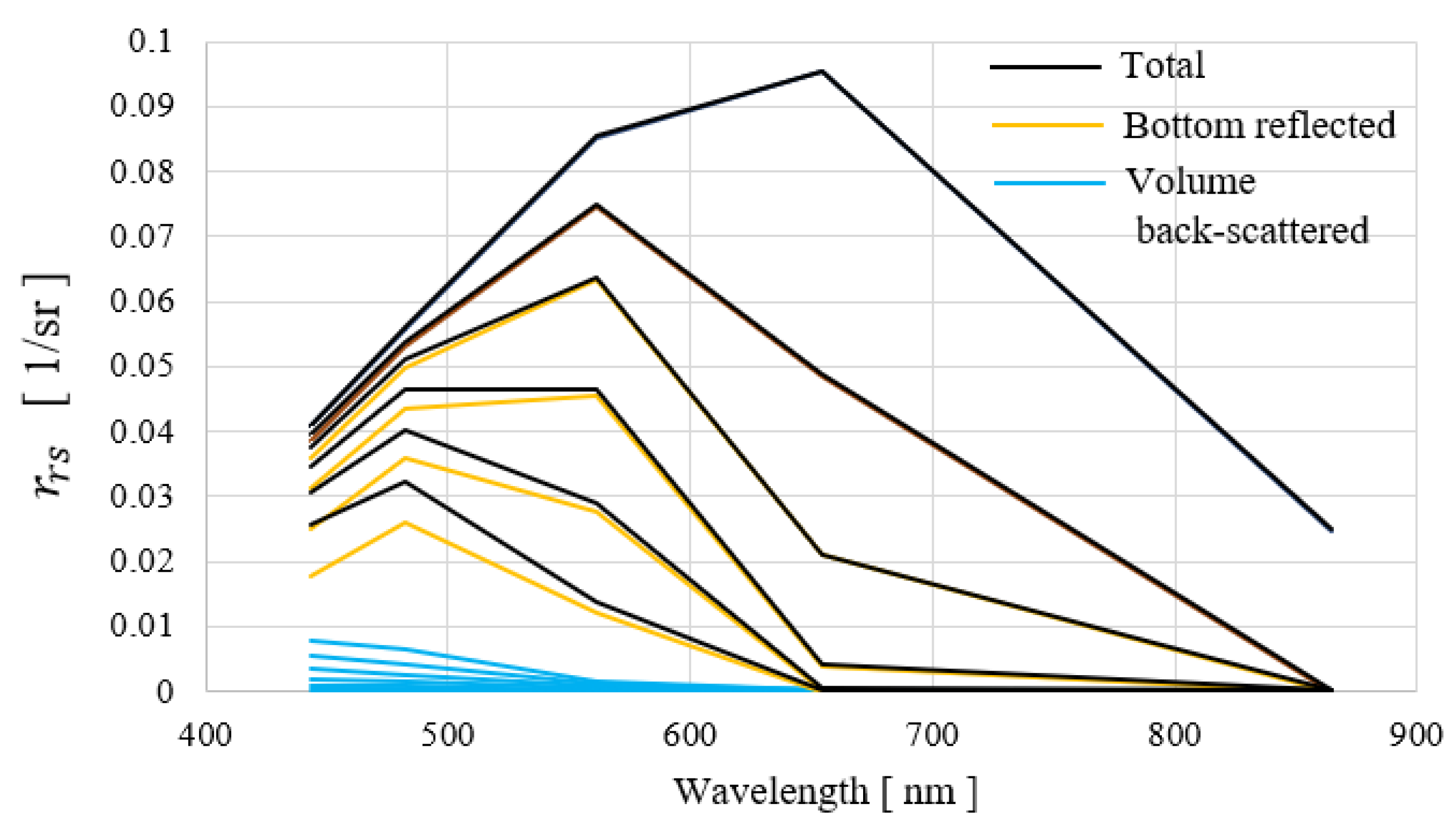
2.5.1. Reflectance Model of Optically Shallow Coastal Water

The ocean optical reflectance equation is given by [1]:

$$r_{rs}\left(z\right)=r_{rs,\infty }·\left\{1-\exp \left[-\left( K_u+K_d\right)·z\right]\right\}+({\rho }_b/\pi )·\exp \left[-\left( K_u+K_d\right)·z\right],$$

(19)

The first term represents the subsurface reflectance due to the volume backward scattering portion, and the second term represents the bottom reflected portion. The term $r_{rs,\infty }$ represents the reflectance from optically deep water, where all the reflectance comes from the optical interaction of sunlight with the water volume. The ${\rho }_b/\pi$ term represents the bottom reflection. When the water depth $z$ varies from very shallow to deep, the exponential term “exp[]” varies from unity to zero. Accordingly, the term “1 − exp[]” varies from zero to unity. Thus, in shallow water, the first term is negligibly small, and the second term dominates. In deep water, the first term dominates, and the second term becomes negligible. The change in magnitude of the first term (cyan-colored curves in Figure 3) and second term (yellow-colored curves) happens in exponential fashion, and the sum of two terms (black-colored curves) also shows exponential decrease, which is demonstrated in Figure 3.

2.5.2. Bottom Reflectance Modeling

The unknown bottom reflectance of a pixel is a vector with $N_w$ elements. The depth of the water is another unknown parameter. Thus, even after reduced unknowns using assumptions, the number of known values, which is the $N_w$-element reflectance spectrum, is always smaller than the number of unknown parameters. Thus, one must handle the bottom reflectance in a different manner to make the optimization solution possible. Most bottom types are sand-like or grass-like. The sand-like bottom includes bright ooid sand, quartz sand, mixed muddy sand, and even muds. Each type of sand and mud also has a wide variety of brightness. The grass-like bottom is also a broad category that includes bottom algae coating, seagrass, and macrophytes. It also could be green algae, red algae, and even various kinds of coral because the multispectral band data usually do not reliably differentiate them. Several bottom spectra measured from various inland and coastal zones, including the bottom spectra collected at Lee Stocking Island, Bahamas [20], are presented in Figure 4.

To make the optimized solution possible, one assumes that the bottom reflectance is a linear mixture of two types of bottoms: sand-like and grass-like.

$${\rho }_b=C_s·{\rho }_{bs}+C_g·{\rho }_{bg}$$

(20)

Ideally, the bottom reflectance coefficients should satisfy the unity condition, $C_s+C_g=1.$ However, when an unknown bottom is modeled using a certain preselected and predefined library, the unity condition is not realistic. Thus, it is reasonable to relax the condition so that more flexible $C_s,C_g$ parameters fit the total reflectance better. Regardless of the specifics of bottom modeling, the essence is that the number of unknowns is reduced from $N_w$ to just two, which allows for numerical optimization.

2.5.3. Nonlinear Optimization for SDB Solution

The parameter vector for SDB is renamed for notational simplicity.

$$\mathit{P}=\left[S,G, z\right]\equiv \left[{\mathit{C}}_{\mathit{s}}, {\mathit{C}}_{\mathit{g}}, \mathit{z}\right]$$

(21)

The optimization to minimize the error for the numerical equation is defined as follows:

$$Find \mathit{P} that minimizes ‖\mathit{w}·\mathit{e}‖, e\left(\lambda ;\mathit{P}\right)=r_{rs,0}\left(\lambda \right)-r_{rs}\left(\lambda ;\mathit{P}\right)$$

(22)

Three columns of the Jacobian matrix for each parameter are expressed as:

$$\begin{gathered} \mathit{J}\left({\Phi }_S;\lambda \right)\equiv \frac{\partial r_{rs}}{\partial {\Phi }_S}=\frac{\partial r_{rs}}{\partial C_s}·\frac{\partial C_s}{\partial {\Phi }_S} \\ =\left(\frac{{\rho }_{bs}}{\pi }\right)· \exp \left[-\left( K_u+K_d\right)·z\right]·\frac{S_{min}-S_{max}}{2}·\mathrm{s}\mathrm{i}\mathrm{n}{\Phi }_S, \end{gathered}$$

(23)

$$\begin{gathered} \mathit{J}\left({\Phi }_G;\lambda \right)\equiv \frac{\partial r_{rs}}{\partial {\Phi }_G}=\frac{\partial r_{rs}}{\partial C_g}·\frac{\partial C_g}{\partial {\Phi }_G} \\ =\left(\frac{{\rho }_{bg}}{\pi }\right)· \exp \left[-\left( K_u+K_d\right)·z\right]·\frac{G_{min}-G_{max}}{2}·\mathrm{s}\mathrm{i}\mathrm{n}{\Phi }_G , \end{gathered}$$

(24)

$$\begin{gathered} \mathit{J}\left({\Phi }_z;\lambda \right)\equiv \frac{\partial r_{rs}}{\partial {\Phi }_z}=\frac{\partial r_{rs}}{\partial z}·\frac{\partial z}{\partial {\Phi }_z} \\ =\left( K_u+K_d\right)·\left( r_{rs,\infty }-\left(\frac{{\rho }_b}{\pi }\right)\right)· \exp \left[-\left( K_u+K_d\right)·z\right]·\frac{z_{min}-z_{max}}{2}·\mathrm{s}\mathrm{i}\mathrm{n}{\Phi }_z \end{gathered}$$

(25)

When the bottom reflectance unity condition, $C_s+C_g=1,$ is applied, it becomes a 2-parameter problem. Accordingly, the two Jacobian columns are combined to a single column:

$$\mathit{J}\left({\Phi }_S;\lambda \right)=\left(\frac{{\rho }_{bs}-{\rho }_{bg}}{\pi }\right)· \exp \left[-\left( K_u+K_d\right)·z\right]·\frac{S_{min}-S_{max}}{2}·\mathrm{s}\mathrm{i}\mathrm{n}{\Phi }_S.$$

(26)

Using the Jacobian column, the update of the parameter for the next iteration in the Levenberg–Marquardt nonlinear optimization scheme is made in the same manner as Equation (16).

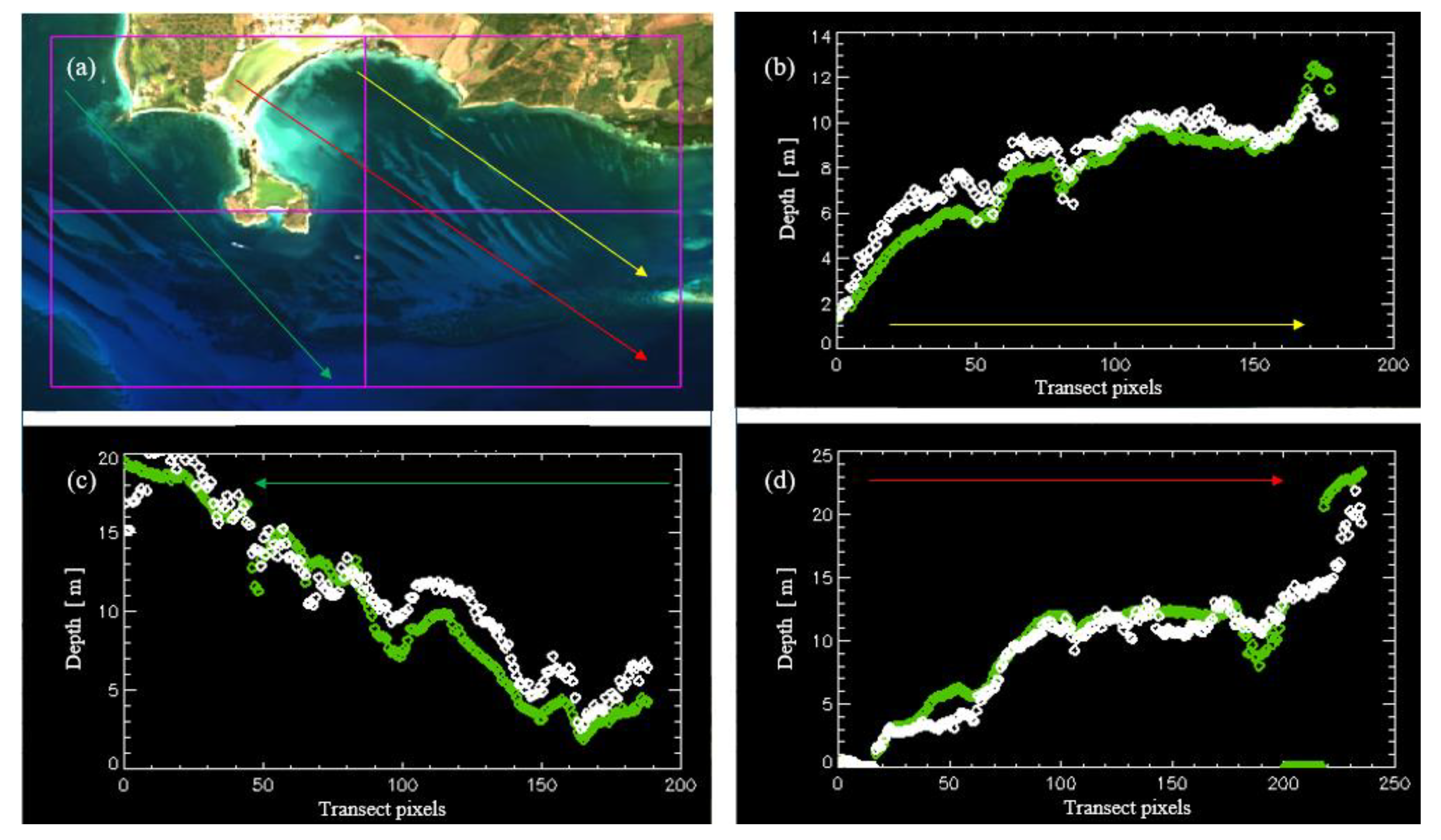
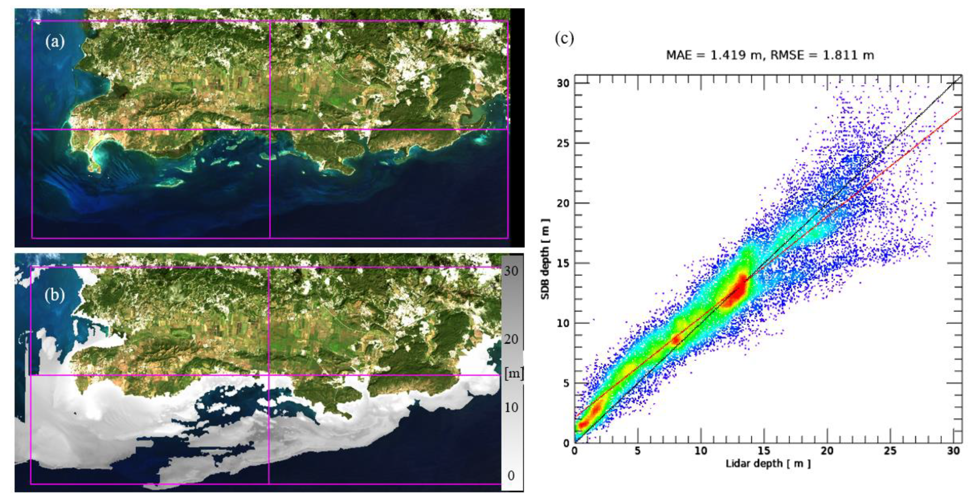
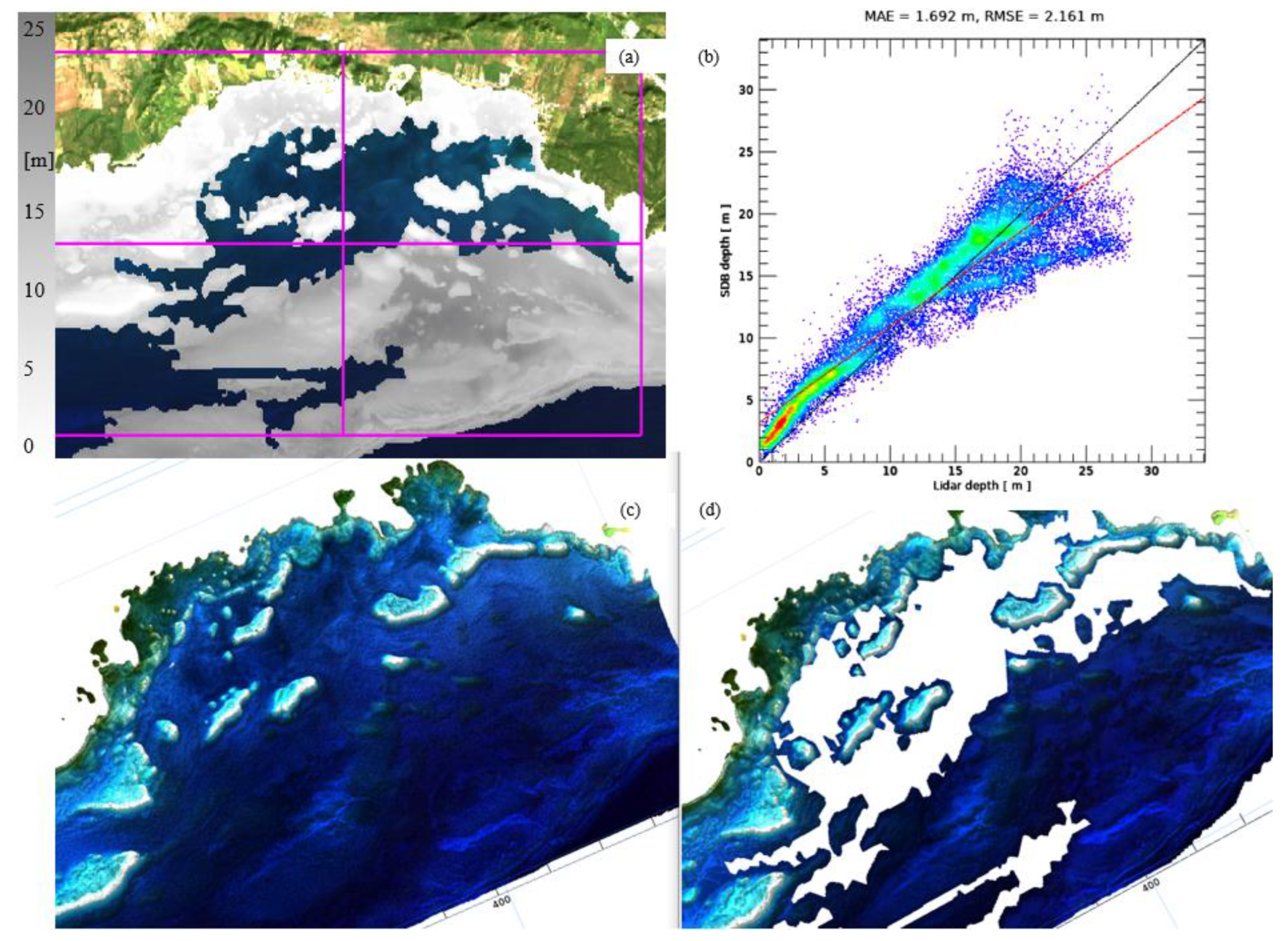
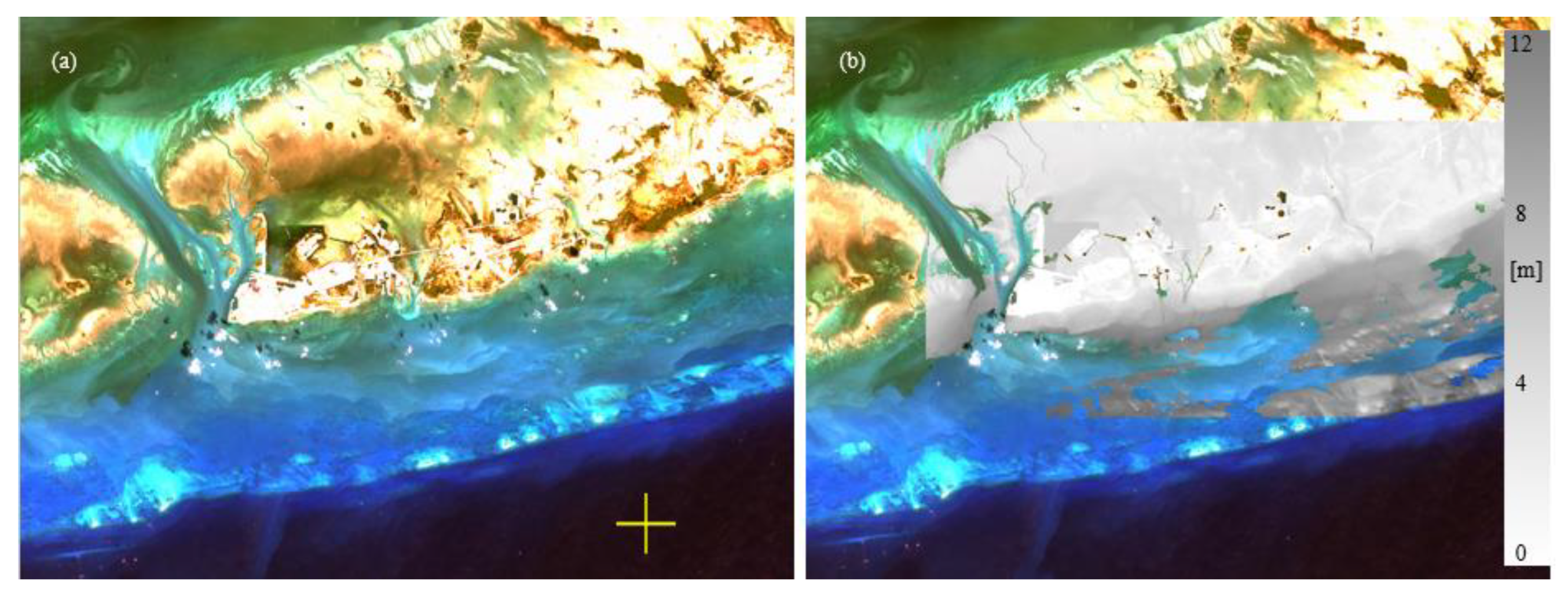
3. Results and Discussion

In this section, the detailed procedure of SDB production is demonstrated step by step. Several Landsat OLI coastal zone images are used, and the available bathymetric lidar data are used as a reference for accuracy assessment. Special attention is paid to the local specific bottom reflectance derived from the combination of the image and lidar data.

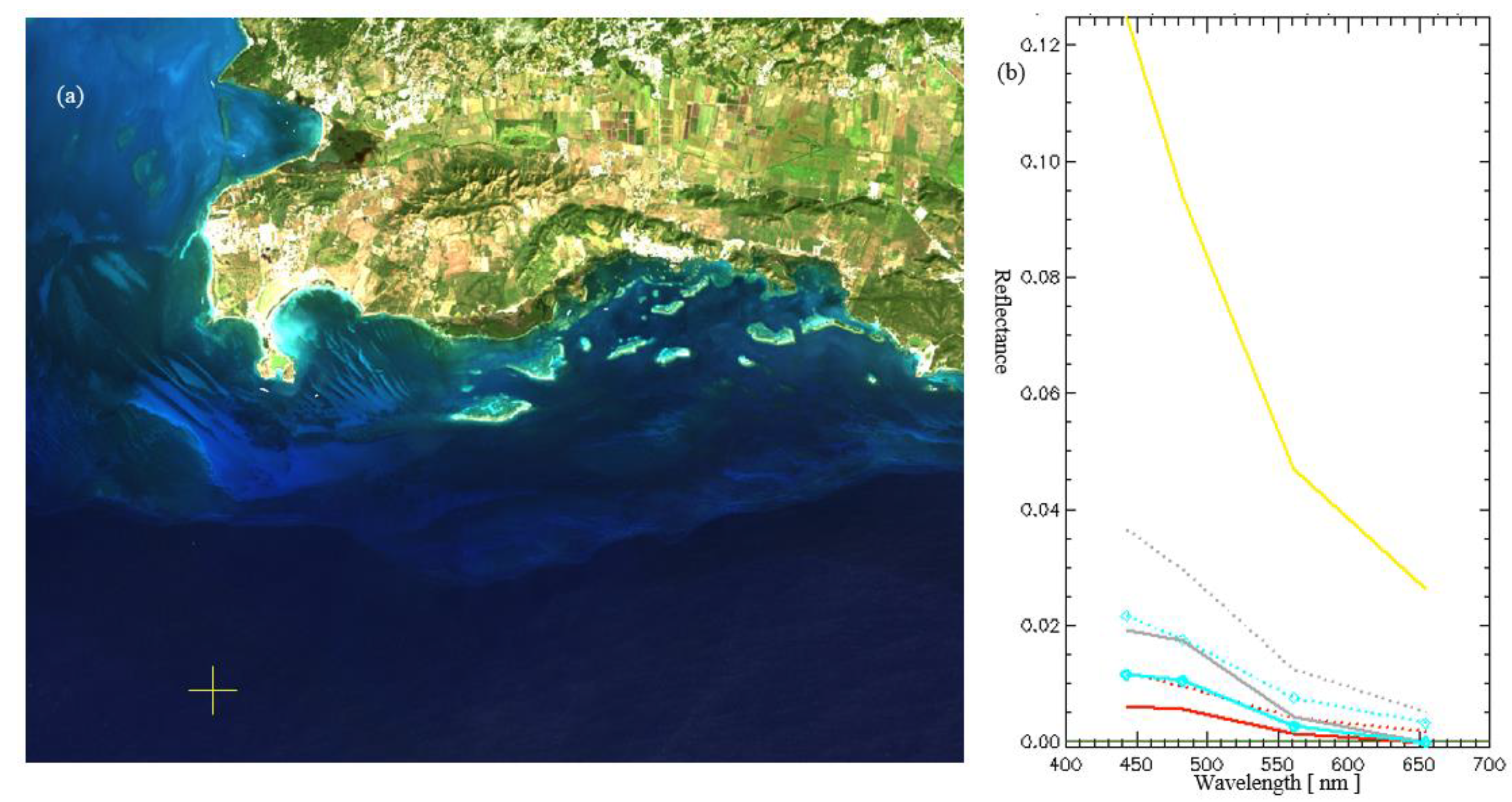
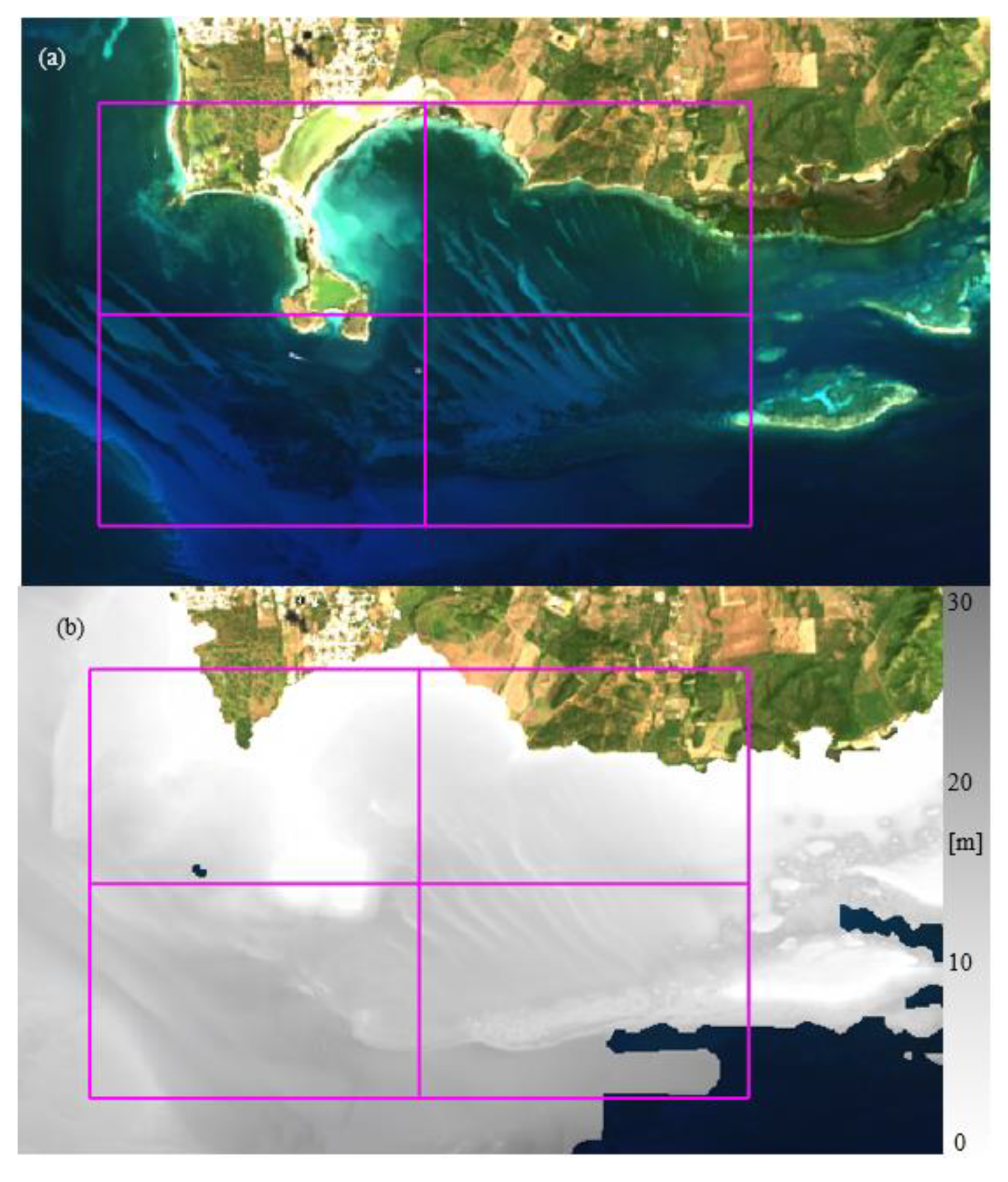
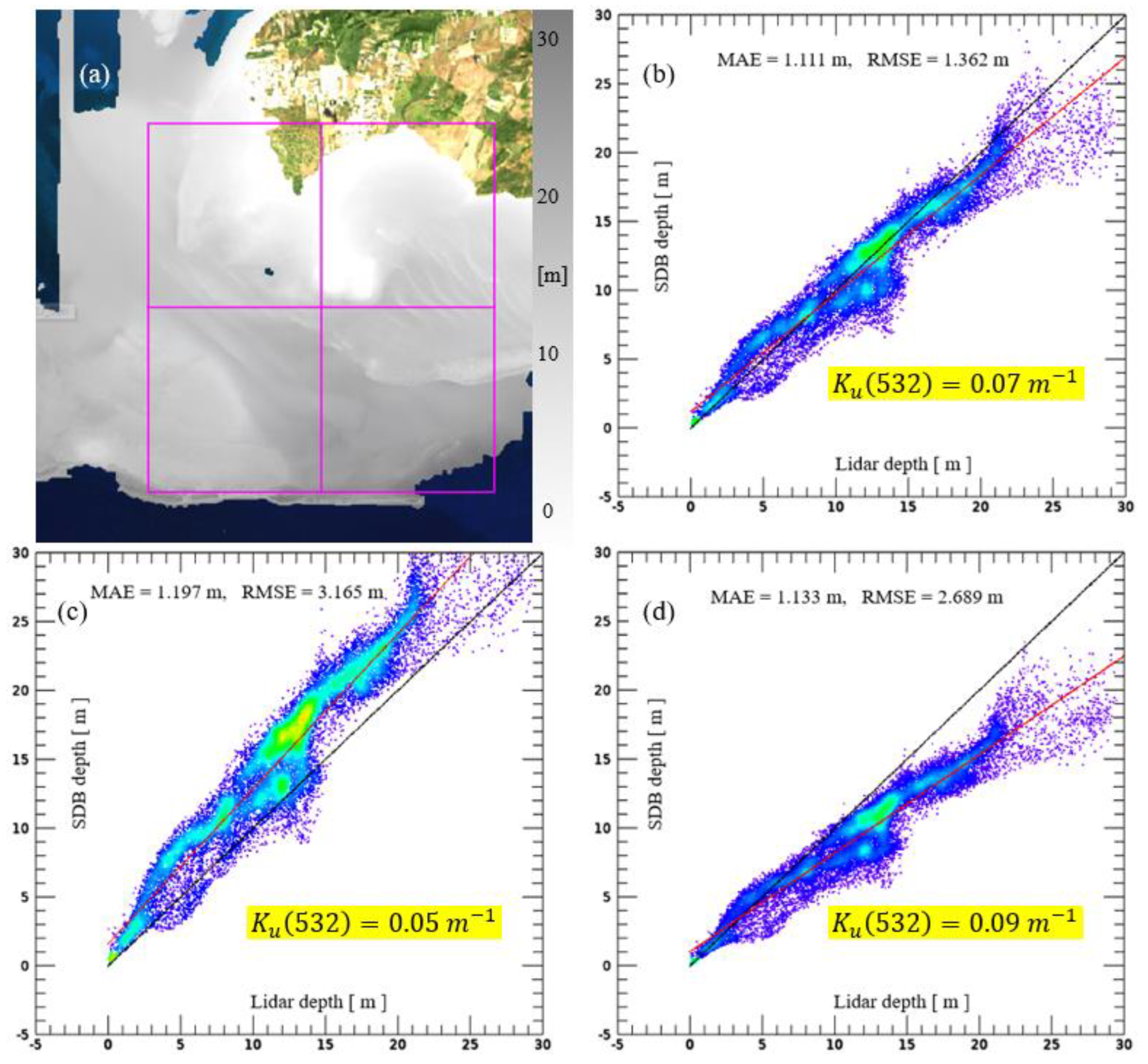
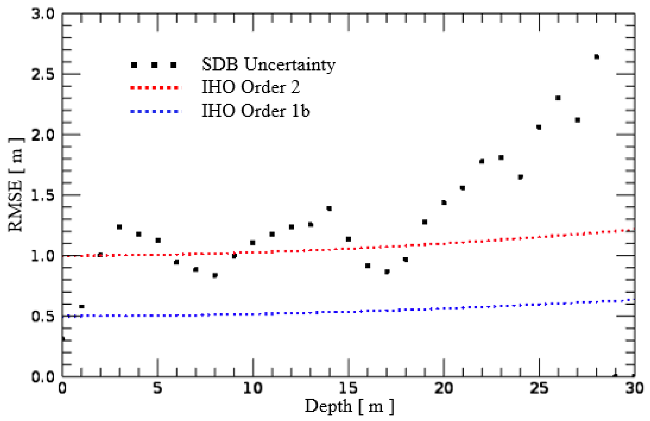
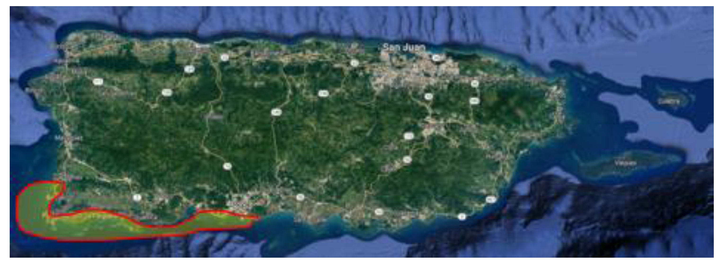
3.1. Study Sites and Validation Data

The study sites are Guam, Key West, and Puerto Rico. The first site, Puerto Rico (LC09_L1TP_005048_20230129_20230129_02_T1), is the cloud-free Landsat OLI scene presented in Figure 5a. Bathymetric lidar data are used as validation data (National Oceanic and Atmospheric Administration National Geodetic Survey). The first step is to sample a spectrum from an optically deep-water area (yellow cross in Figure 5a).

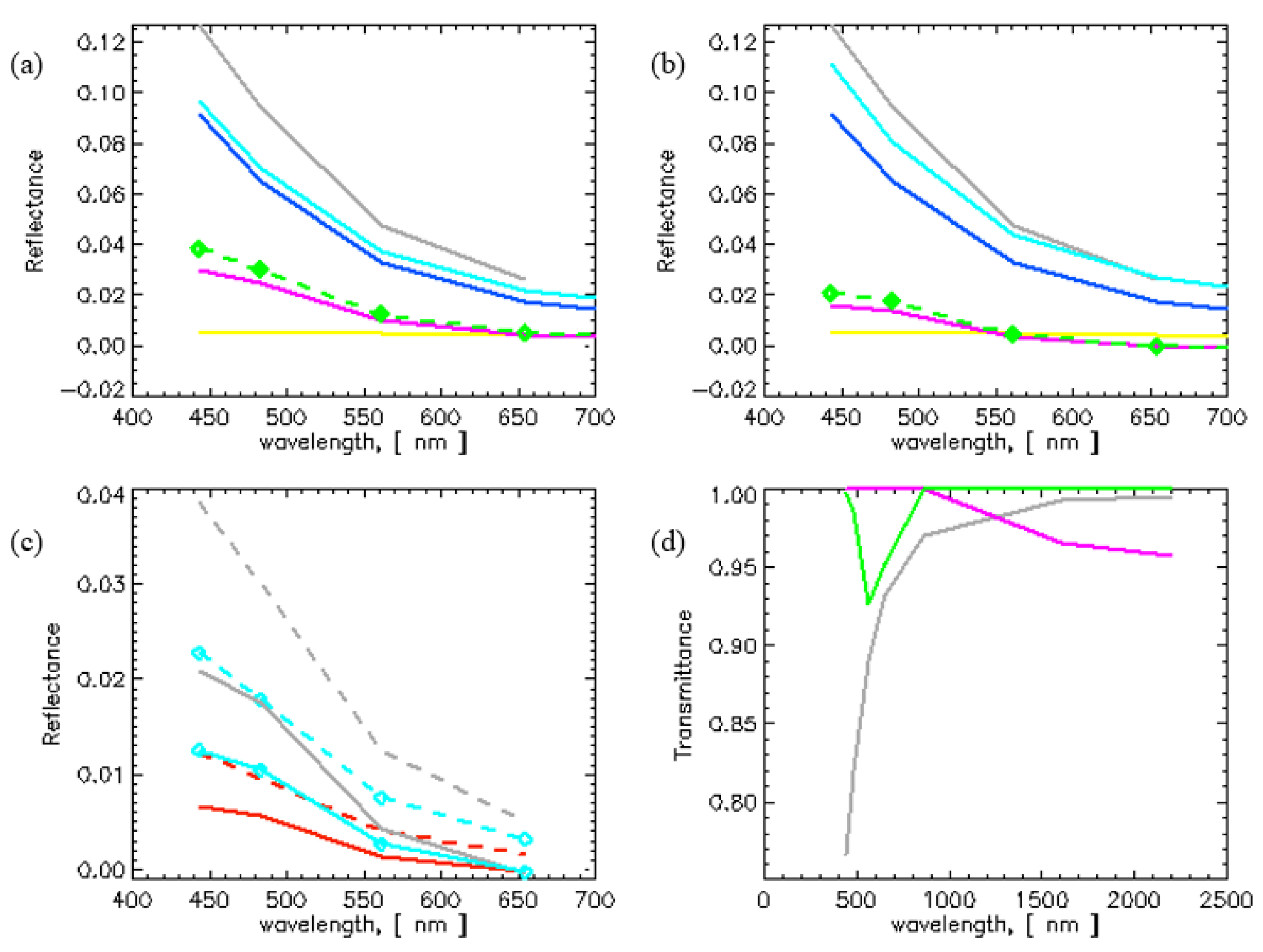
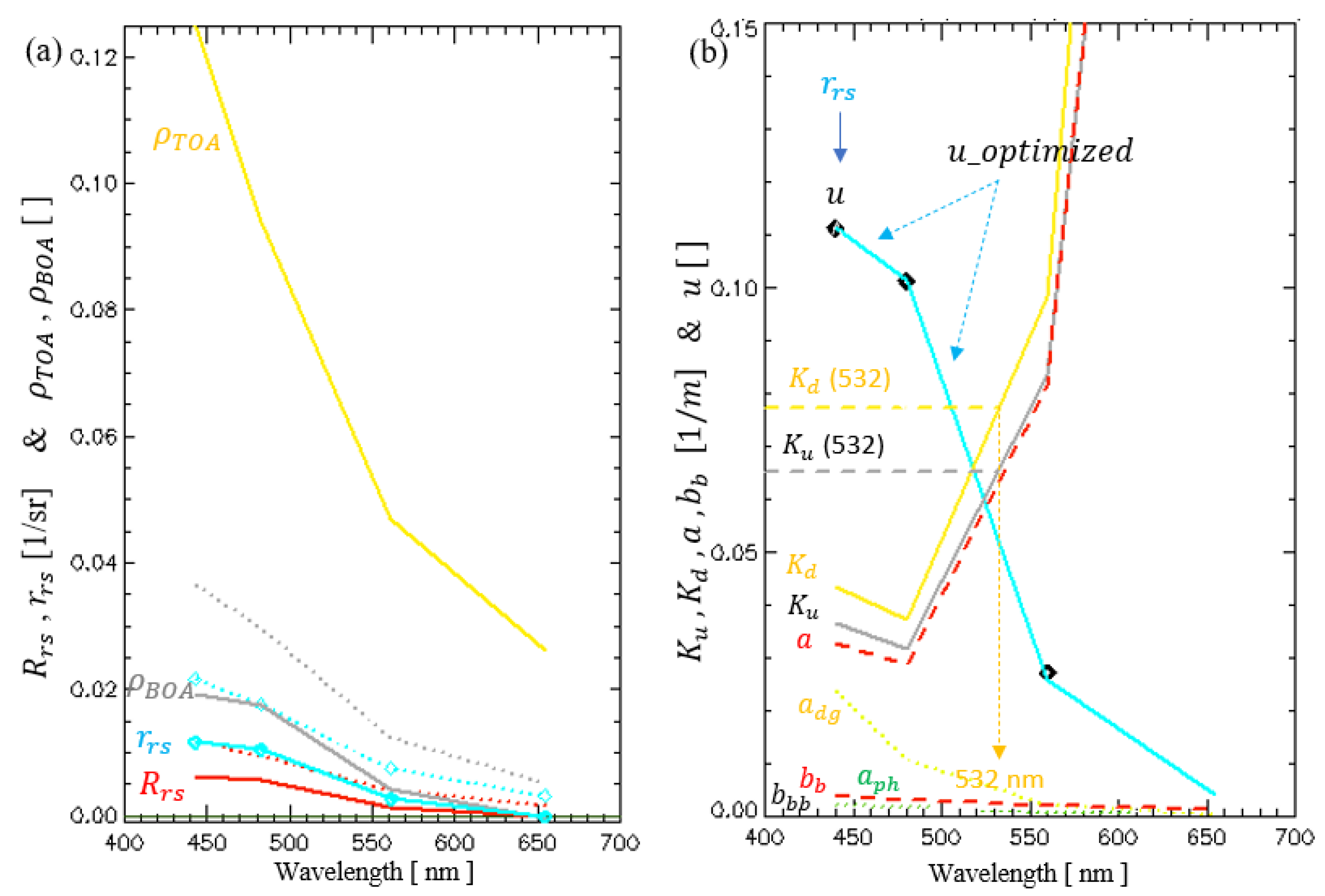
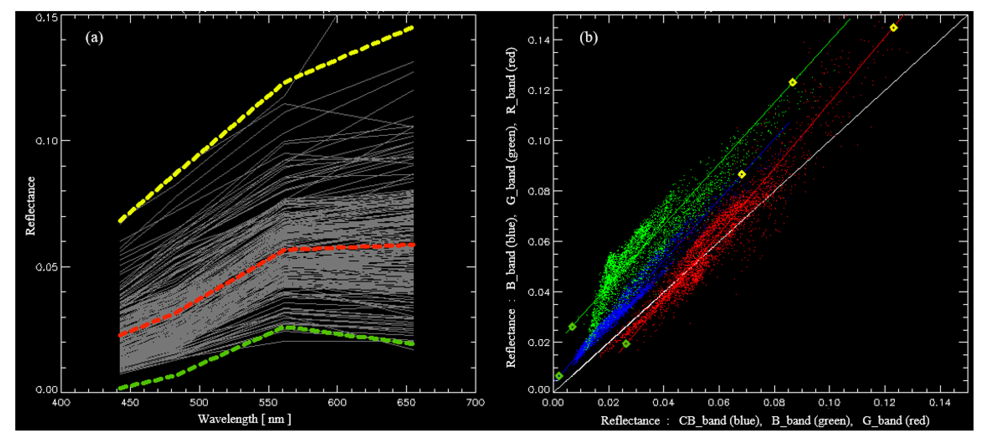
3.2. Atmospheric Correction of Optically Deep Water

The optimal ${\tau }_a$ is determined to satisfy the dark pixel assumption based on Ahmad LUT [12] that considers both atmospheric and surface reflection, as presented in Figure 5b. The dark pixel assumption is that the reflectance of longer wavelengths (red and near-infrared bands) is near zero. On the contrary, reflectance using 6SV LUT [10] does not suppress the longer wavelength bands to zero because the Ahmad model includes a water surface boundary but the 6SV model does not. ${\rho }_{BOA}$ is converted to $R_{rs}$ (red curve) and subsequently to $r_{rs}$ (cyan diamond symbol curve) using Equation (3). The atmospheric correction result of Figure 5b was transferred from Figure 6c. The detailed component of atmospheric correction using 6SV LUT are presented in Figure 6a and the detailed component of atmospheric correction using Ahmad LUT in Figure 6b. Various transmission spectra found in Equation (2) are shown in Figure 6d.

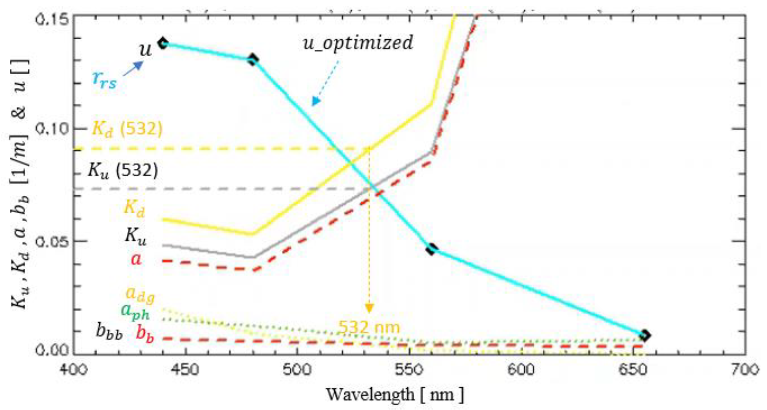
3.3. Inversion of Optical Properties of Water

The conversion of subsurface remote sensing $r_{rs}$ to $u$ and successive optimization via the optical model of the dominant ocean optical components uses Equations (4)–(16). The optimized results associated with $u\_optimized$ in Figure 7b are as follows:

$$b_{bp}\left({\lambda }_0\right)=0.00166 {\mathrm{m}}^{-1}, a_{dg}\left({\lambda }_0\right)=0.01645 {\mathrm{m}}^{-1},C=0.07505 \mathrm{m}\mathrm{g}/{\mathrm{m}}^3$$

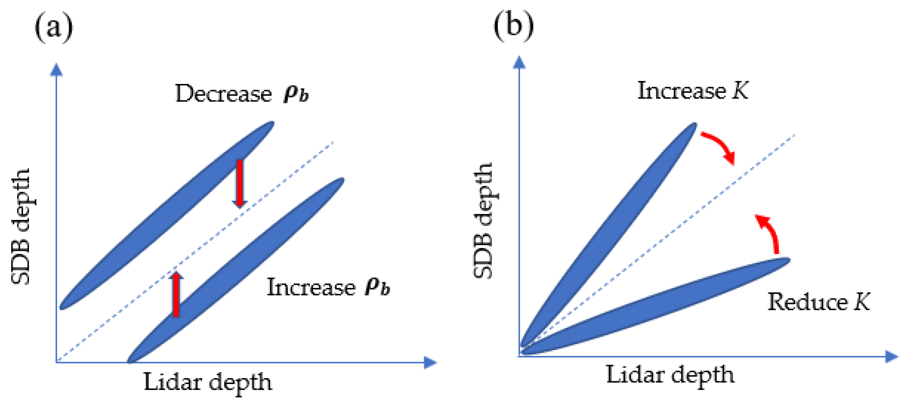
3.4. Effect of Physical Parameters

To demonstrate the effect of various bottom surface types from the bottom reflectance library, the diffuse attenuation coefficients ($K_u, K_d$) are fixed, and the simulated $r_{rs}$ spectra at varying depths (2 m, 5 m, and 15 m) are derived. The SDB algorithm solves for depth and bottom weights for sand-type and grass-type. The effect of water depth leads to the greatest variance, as demonstrated in Figure 8a. We assume the diffuse attenuation coefficient is estimated from the nearby optically deep water, and the optically shallow region is assumed to have the same optical properties. However, the assumption is generally not valid because the different attenuation makes substantial differences, as demonstrated in Figure 8b. Along with depth, the bottom reflectance spectrum is the other apparent factor that results in a wide dynamic range of reflectance, as demonstrated in Figure 8c.

Because the effect of major parameters on the subsurface remote sensing reflectance is substantial and only five OLI bands are available (including the NIR band), reasonable assumptions for atmospheric correction and IOPs were made. At the last step, one still needs to choose the two bottom spectra (sand-like and grass-like) from the library.

3.5. Initial Result

The initial SDB analysis uses the area shown in the box of Figure 9a. Also shown is the bathymetric lidar point cloud in Figure 9b.

The difference between lidar water depth and SDB depth has a mean absolute error (MAE) value of 1.515 m and root mean squared error (RMSE) value of 4.028 m in Figure 10. This result is using the initial choice of the two spectra. The improvement of the bottom spectra is discussed in the next section.

The bathymetric lidar digital elevation model (DEM) (refer to Data Availability Statement at the end) is processed so that it is converted to the lidar water depth as follows. An example OLI image is displayed, and a high spatial resolution topographic–bathymetric digital elevation model (TBDEM) is overlaid as a grayscale image (Figure 11). A TBDEM is defined under a specific datum, whereas SDB estimates water depth where the reference water surface is variable depending on the time of the day. Thus, it is necessary to find an offset to the water surface level at the time of satellite overpass. Over the overlapping region between the image and DEM, each pixel is evaluated as to whether the pixel spectrum has a spectral property of a typical water pixel. The boundary line between the two different pixel types gives a proper DEM offset to water depth. In this example, −0.35 m was the offset. Thus, we subtract −0.35 m from the raw DEM so that −0.35 m becomes the zero water level, and then the sign is changed to be the physical depth. This is the lidar water depth that is compared to the SDB depth.

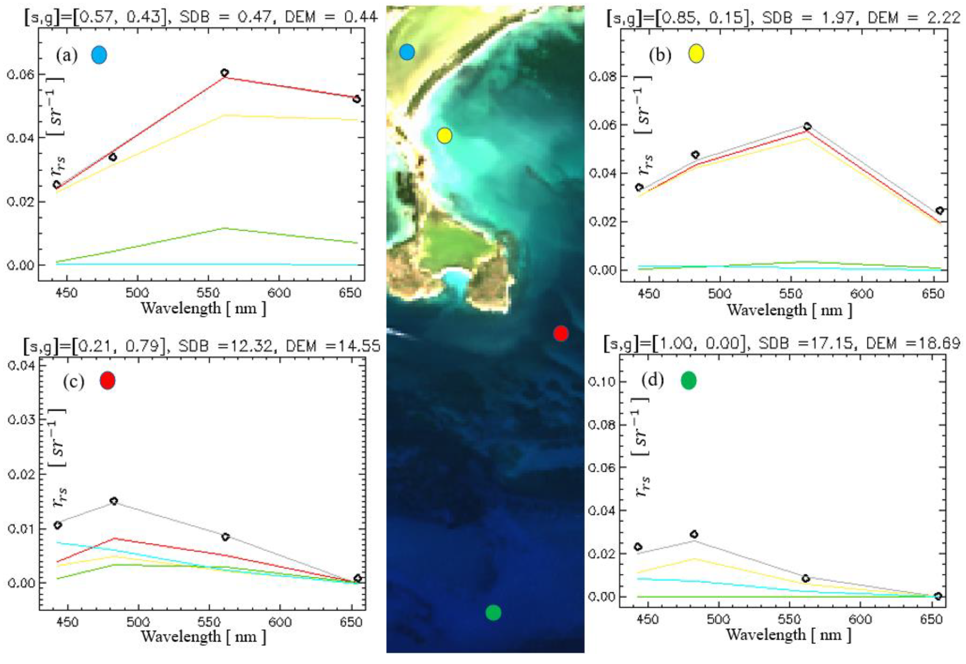
3.6. Estimation of Scene-Derived Bottom Reflectance

The objective of this phase of the workflow is to reduce the effect of uninformed choice of bottom reflectance library on the SDB result. When a reference lidar depth is available, it is possible to estimate scene-derived bottom reflectance. When the scene-derived sand-like and grass-like library is used, the SDB optimization would be more accurate because the reduced uncertainty of linear mixture bottom modeling would increase the accuracy of depth optimization. The subsurface reflectance is related to the bottom reflectance multiplied by an exponential term, so increasing depth results in exponentially decreasing bottom reflected signal. Thus, it is desirable to limit the sampling region to very shallow water. In this research, we sample the shallow water spectrum from less than 2 m in depth (Figure 12).

Assuming the water volume reflectance is negligible in shallow water, the first term of Equation (19) is negligible. The second term is dominated by the bottom reflectance as the exponential term is substantially larger because the small optical depth in the exponent makes the exponential term comparable to unity. Equation (19) is simplified and is rearranged for total bottom reflectance:

$${\rho }_b=\pi ·r_{rs}\left(z\right)·\exp \left[\left( K_u+K_d\right)·z\right]$$

(27)

Applying the shallow pixels to Equation (27), an $N_w\times N$ matrix $\left[{\mathit{\rho }}_{\mathit{b}}\right]$ is created, where $N$ is the number of pixels. The $N$ inverted bottom spectra are provided in Figure 12a. The lower inverted spectra are closer to pure grass-like spectra, while the upper spectra are closer to sand-like spectra. Simply picking the minimum and maximum spectra would not work in general because an individual inverted spectrum is not likely to represent the endmembers. We suggest that the proper approach is to use eigenanalysis. For eigenanalysis, a covariance matrix needs to be calculated first. Using the $N_w\times 1$ bottom reflectance vector $\overline{{\rho }_b}$, a covariance matrix $\mathit{\Sigma }$ is computed:

$$\mathit{\Sigma }=\left({\mathit{\rho }}_{\mathit{b}}-\overline{{\rho }_b}\right) ·{\left({\mathit{\rho }}_{\mathit{b}}-\overline{{\rho }_b}\right)}^T$$

(28)

The bottom reflectance estimated using Equation (27) is assumed to be a linear mixture from sand-like and grass-like pure endmembers. The eigenanalysis of the covariance matrix provides a way to estimate the unknown endmember pixel spectra. The first eigenvector ${\mathit{v}}_1$ with the largest eigenvalue ${\lambda }_1$ is computed from the covariance matrix $\mathit{\Sigma }$. The first eigenvector describes the greatest variance in the $N_w$ dimensional space. Each mean-shifted vector $({\rho }_b-\overline{{\rho }_b})$ can be projected to the first eigenvector ${\mathit{v}}_1$. Mathematically, the result is computing the inner product:

$$k=\left({\rho }_b-\overline{{\rho }_b}\right) ·{\mathit{v}}_1$$

(29)

Because the number of ${\rho }_b$ is $N$, the number of scalar values $k$ is also $N$. The two end points along the first eigenvector in the multi-dimensional space are assumed to be the vector to the two pure endmember spectra. One needs to specify how to determine the end points. Because the data are mean shifted, the projection $k$ will have either positive or negative values. The ${\rho }_b$ spectra with positive $k$ values are mostly on the sand-like bottom side, and ${\rho }_b$ spectra with negative $k$ values are mostly on the grass-like bottom side.

The way to specify the endmembers is to assign the proper $k$ value. Simply assigning $k_{max}$ for sand-like endmembers and $k_{min}$ for grass-like endmembers is not a desirable strategy because the distribution of $k$ values from a natural shallow bottom is likely to be biased, or there is a high chance that the pure endmember may not exist in the sampled pixels. Thus, determining $k_s$ for sand-like endmembers and $k_g$ for grass-like endmembers always involves some level of ambiguity. We suggest using the lower 5% and upper 95% of the $k$ value range as initial values of $k_g$ and $k_s$, respectively, and calculating the endmembers ${\rho }_{bg}$ and ${\rho }_{bs}$:

$${\rho }_{bg}=k_g{\mathit{v}}_1+\overline{{\rho }_b}, {\rho }_{bs}=k_s{\mathit{v}}_1+\overline{{\rho }_b}$$

(30)

The estimated ${\rho }_{bg}$ and ${\rho }_{bs}$ spectra may then be evaluated to see if they have desirable properties as endmembers: whether they have similarity with typical grass-like and sand-like spectra, whether they are located at the end region in the distribution, or whether they are not extreme outliers. There is no unique solution, but rather a user may use discretion based on experience in adjusting $k_g$ and $k_s$. The ${\rho }_{bg}$ and ${\rho }_{bs}$ spectra finally estimated in this example are displayed in Figure 13a. Because the distribution of four-dimensional ${\rho }_b$ data is not possible to visualize, Figure 13b shows two-dimensional plots of three band pairs.

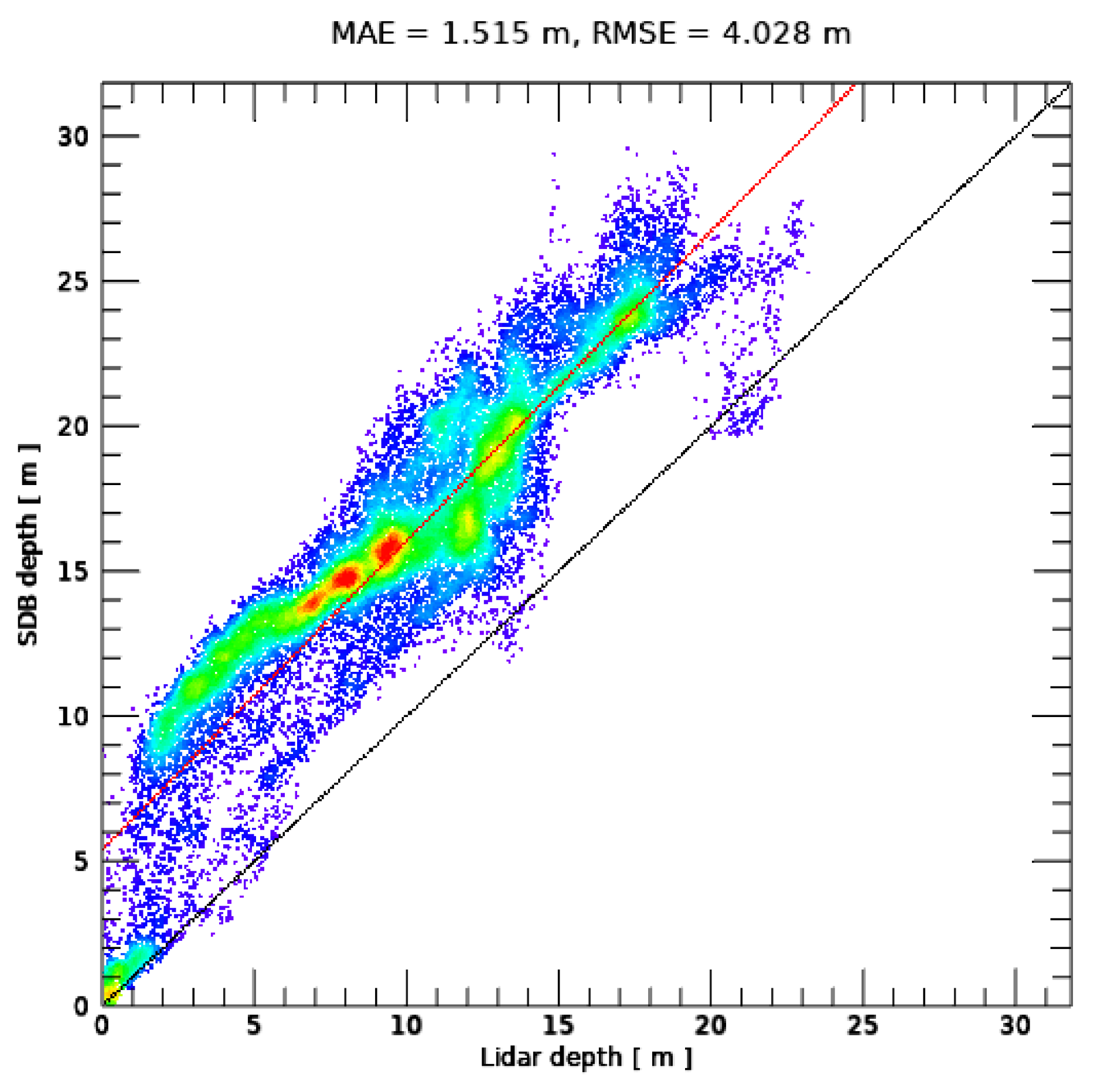
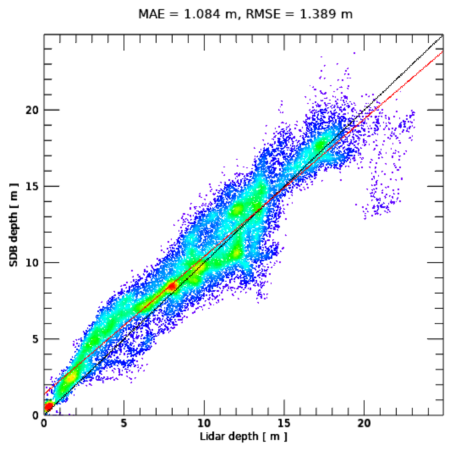
3.7. SDB Result Using Scene-Derived Bottom Reflectance Endmember

The same image region (Figure 9a) is used for SDB computation using scene-derived bottom reflectance endmembers. The depth scatterplot is provided in Figure 14. Noticeable improvement is observed with a much lower RMSE value of 1.57 m. The three-dimensional (3D) visualization of SDB is displayed in Figure 15a, and the 3D bathymetric lidar is shown in Figure 15b.

The SDB optimization result was evaluated at an individual pixel level. Four pixels were sampled, considering varying depths and bottom types. The optimization results for each sample are displayed in Figure 16. The first data (Figure 16a) are sampled from a very shallow area; thus, overall reflectance is highest, and even at the red band, reflectance is substantially higher. At about the 2 m depth region (Figure 16b), the reflectance at the red band is reduced substantially. In the shallow region, the bottom reflected component is dominant. Thus, the red curve explains almost all the total reflectance, and the cyan curve is virtually zero. In the deep-water area, the cyan curve contributes a relatively large amount to the total reflectance. The depth profiles along the three arbitrary lines are shown in Figure 17.

When the SDB calculation is made over a full area where the lidar TBDEM is available, the result is presented in Figure 18.

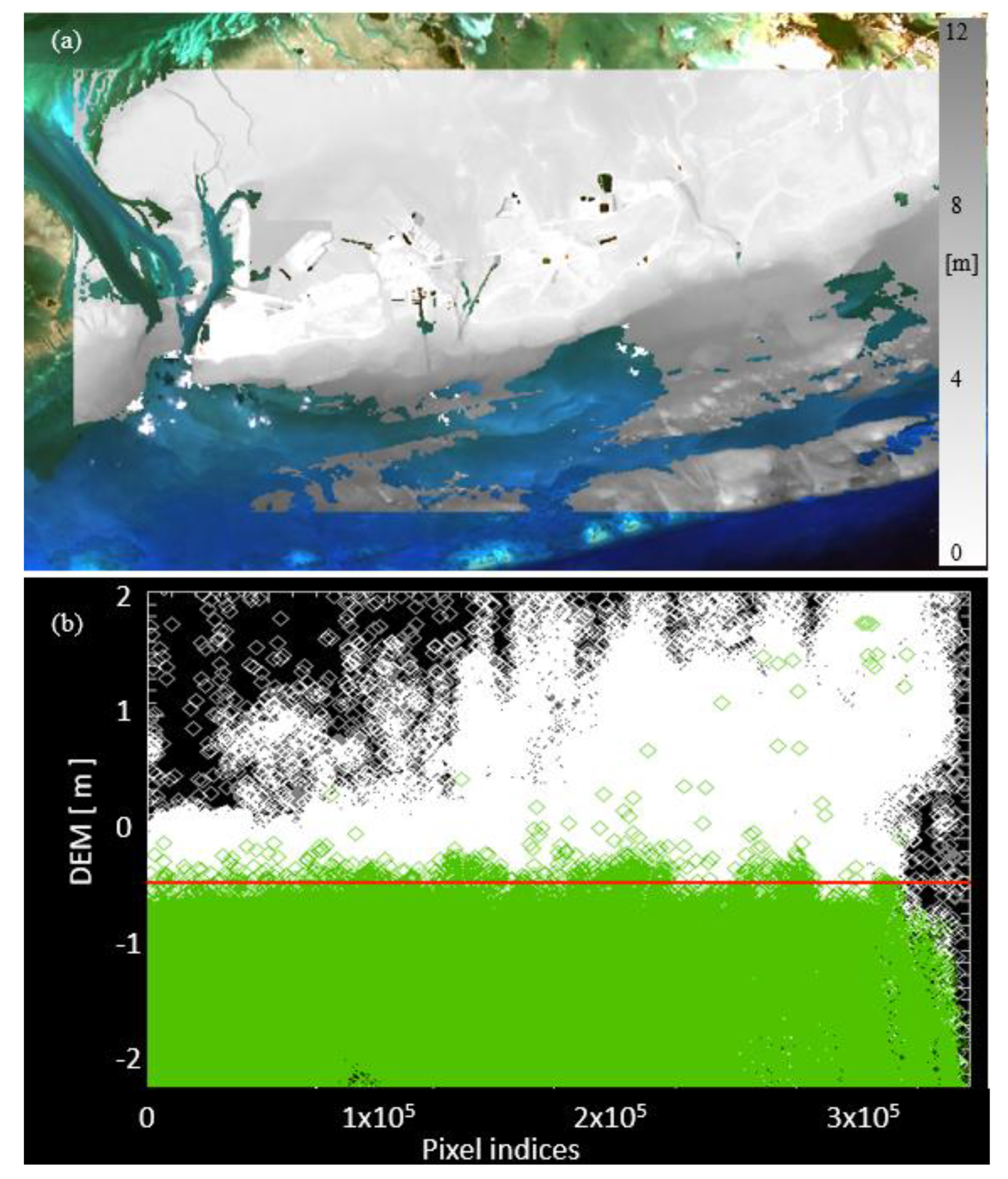
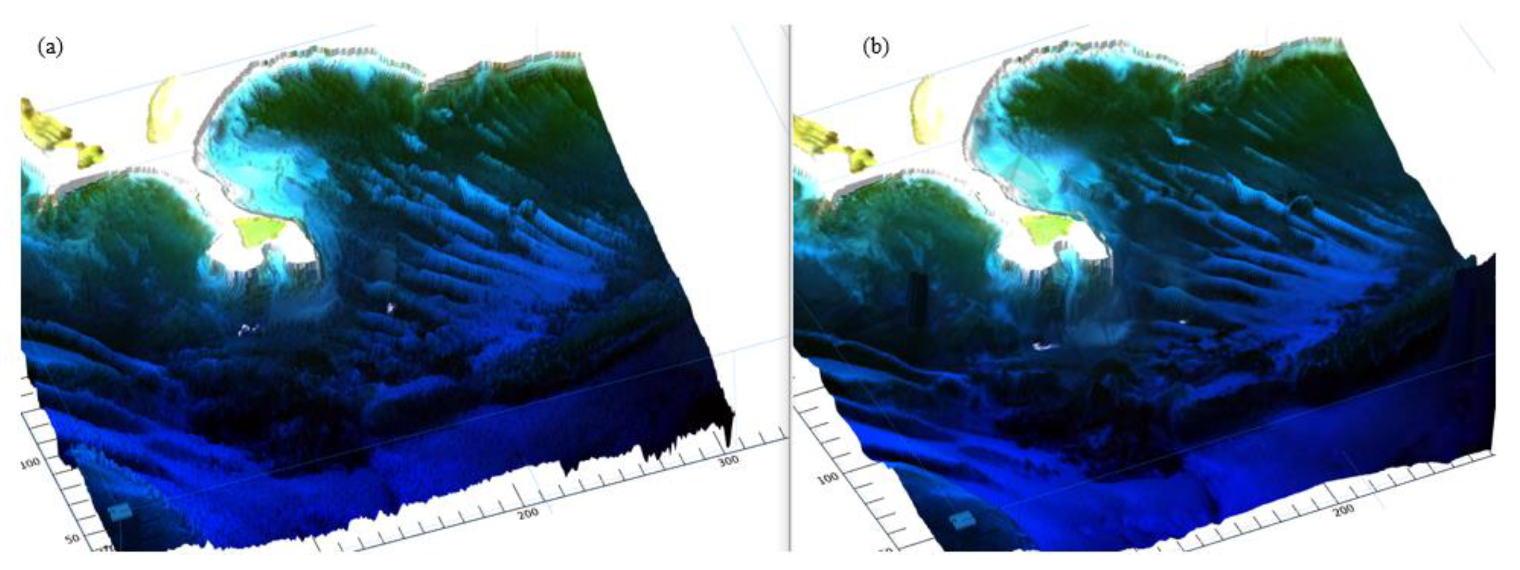
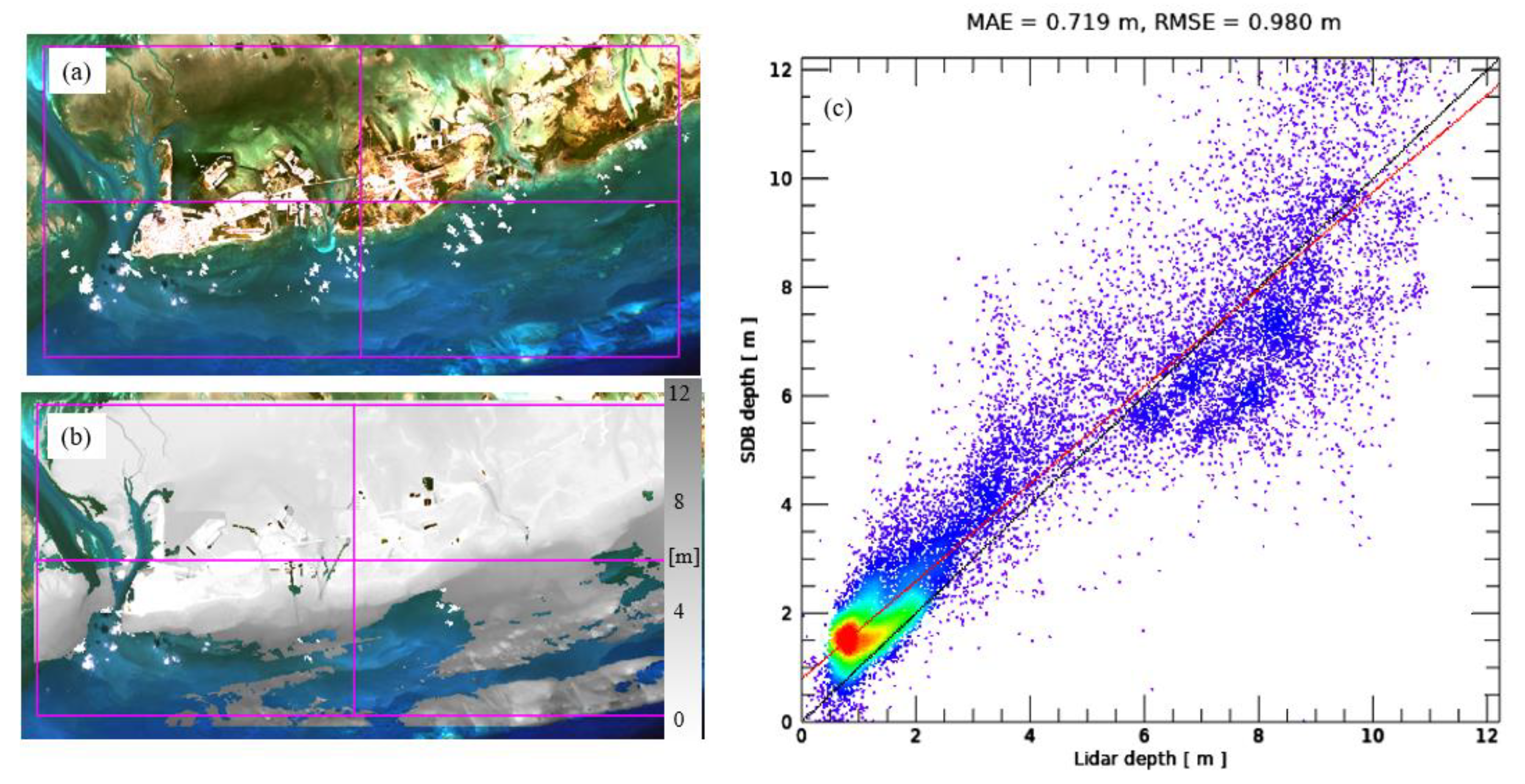
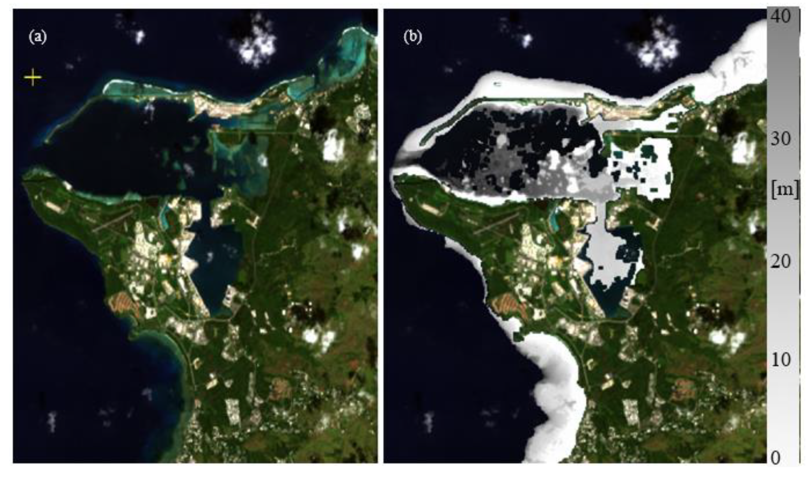
3.8. SDB over Incomplete or Missing DEM Area

Once it is confirmed that the scene-derived bottom works well, one may run SDB for any coastal zone in the image. An image area with incomplete or missing DEM is presented in Figure 19a. Bathymetric lidar failed to detect the bottom return peak from the waveform. The failure does not appear to be because the missing DEM area is too deep to detect the bottom. Regardless of the reason, SDB can invert any pixel to a depth if the area is optically shallow with the optical depth less than 3. The depth scatterplot after SDB shows a relatively low RMSE of 2.16 m (Figure 19b). The 3D visualization of the SDB result is presented in Figure 19c, and the 3D visualization of lidar DEM is shown in Figure 19d, which has a large area of missing lidar data. This result demonstrates that the SDB method presented here has a great advantage over lidar when generating a continuous full 3D view of the sea floor using subsurface reflectance images with the absence of cloud-covered pixels, although the lidar depth precision (about 20 cm) is superb compared to the SDB precision (about 2 m). The essence of the method is that once it is fine-tuned using partial lidar data, this method can produce the SDB of a much larger area.

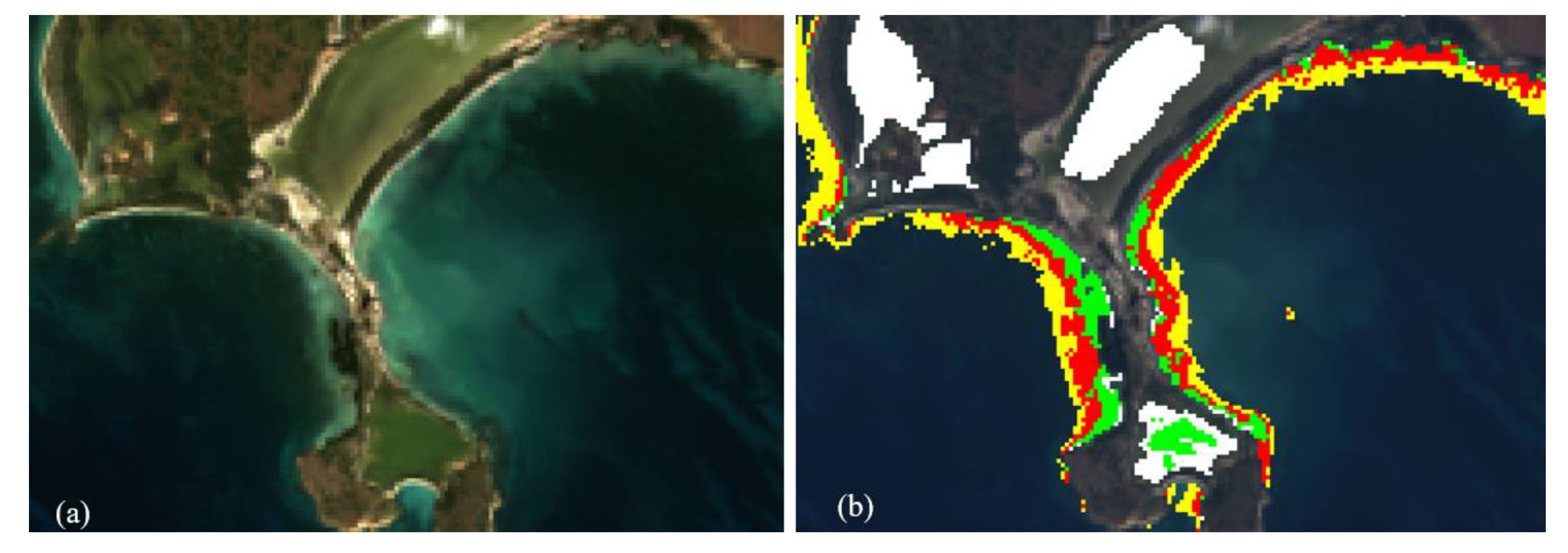
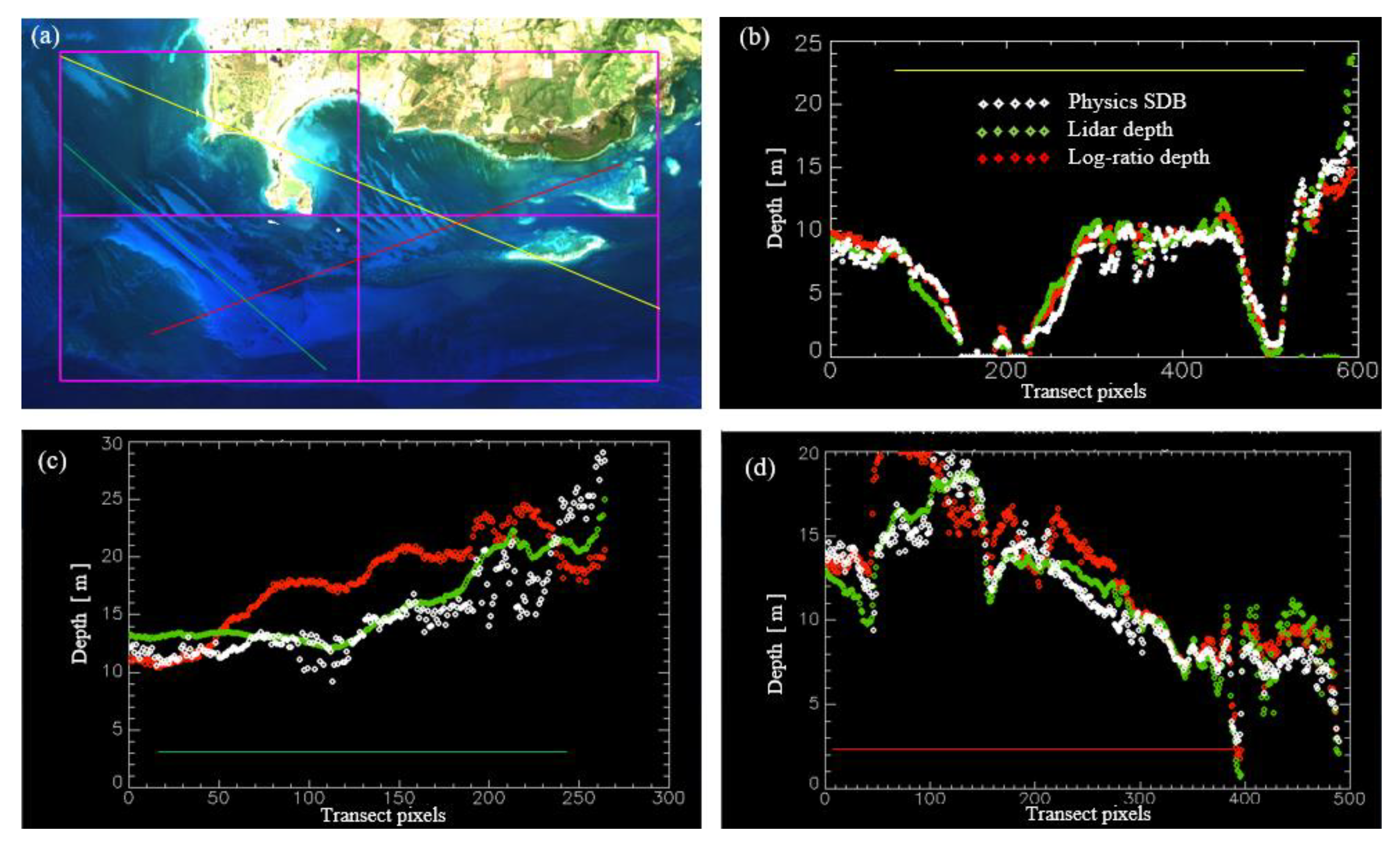
3.9. Additional Examples of SDB

The physics-based SDB algorithm was also applied to Key West, Florida, USA. The relatively cloud-free Landsat OLI scene “LC09_L1TP_016043_20221209_20221209_-02_T1” is shown in Figure 20a. Also available are the topographic–bathymetric lidar data (Figure 20b). The bathymetric lidar data have substantial areas missing. The optically deep water where a pixel spectrum was sampled for atmospheric correction and IOP estimation is presented in Figure 18a. Following the steps of spectral processing explained above, ${\rho }_{BOA}$ is obtained after atmospheric correction of ${\rho }_{TOA}$. Then, ${\rho }_{BOA}$ is converted to $R_{rs}$ and subsequently to $r_{rs}$. The next step is to convert $r_{rs}$ to $u$ (Figure 21). After the optimization, the green line models the optimized $u$ curve and fits the $u$ derived from optically deep water with minimal error. The IOPs of Key West on this day are almost identical to the result from the Puerto Rico scene. The optimization results are as follows:

$$b_{bp}\left({\lambda }_0\right)=0.00249 {\mathrm{m}}^{-1}, a_{dg}\left({\lambda }_0\right)=0.01176 {\mathrm{m}}^{-1},C=0.19835 \mathrm{m}\mathrm{g}/{\mathrm{m}}^3.$$

The associated angles for computing $K_u, K_d$ of the pixel location are SZA = 51.3° and VZA = 2.3°. The rectangular extent of SDB processing on the OLI image and lidar TBDEM is presented in Figure 22a,b. The SDB results have an MAE value of 0.72 m and an RMSE value of 0.98 m (Figure 22c). Most points are in the shallow region of Key West.

Physics-based SDB was also applied to the island of Guam. The Landsat OLI scene “LC08_L1TP_100051_20211109_20211117_02_T1” is presented in Figure 23a. Also available are the bathymetric lidar DEM data (Figure 23b). The bathymetric lidar data have substantial areas missing. Following the steps of spectral processing explained above, the following sequence of conversion happens: ${\rho }_{TOA} \to {\rho }_{BOA} \to R_{rs} \to r_{rs} \to u$. The IOPs of Guam in this image (Figure 24) are much clearer ($K_u\left(532\right)=0.062 {\mathrm{m}}^{-1}$) than those of Puerto Rico or Key West ($K_u\left(532\right)=0.072 {\mathrm{m}}^{-1}$) because Guam is an isolated island at northern Mariana, Pacific Ocean, and the water depth drops off considerably much faster. The optimization results are as follows:

$$b_{bp}\left({\lambda }_0\right)=0.00236 {\mathrm{m}}^{-1}, a_{dg}\left({\lambda }_0\right)=0.00470 {\mathrm{m}}^{-1},C=0.06541 \mathrm{m}\mathrm{g}/{\mathrm{m}}^3.$$

The associated angles for computing $K_u, K_d$ of the pixel location are SZA = 37.1° and VZA = 2.8°. The SDB scatterplot shows an RMSE value of 7.87 m (Figure 25a). The 3D visualization of SDB, which is a full 3D continuous sea floor view, is presented in Figure 25b, whereas the lidar DEM indicates some missing areas in Figure 25c. The result in the error plot (Figure 25a) shows a failure region that is rather flat and away from the one-to-one line. A polygon is selected (Figure 26a), and we visualize where the problematic region is in the image (Figure 26b). The failure region is clearly within the deep bay area. The rest of the coastal region seems better. We believe the bottom type is likely to be a dark volcanic rock, but it seems the deep inner harbor has a peculiar bottom type that causes failure in SDB using generic bottom endmembers. In this exceptional case, SDB needs more fine-tuning using local data.

To perform fine-tuning, without having additional ground truth, one applies a straightforward adjustment. A secondary problem arising from the initial issue is the high MAE value, where SDB substantially overestimates the depth. A major reason for the depth overestimation could be the inaccurate bottom reflectance. If the new bottom input was darker than the initial input, the newly optimized SDB would be shallower. Thus, a scale factor of 0.3 was applied to the initial sand and grass bottom reflectance. Because volcanic rock is the origin of the sediment, a low scale factor seems to make sense. The new region of interest excluding the inner harbor is presented in Figure 27a, and the overlaid TBDEM is shown in Figure 27b. The scatterplot displays a substantial improvement (Figure 27c). Although the lidar TBDEM covers a very narrow range from the coast (Figure 28b), the SDB depth map (Figure 28a) has greater coverage with better bottom description.

3.10. Fine-Tuning Strategies Using TBDEM

The fine-tuning technique that has the greatest effect on the result would be scene-derived bottom reflectance. The technique using the eigenanalysis from shallow water was described in the previous section. The second strategy is to scale bottom reflectance (Figure 29a). If the initial depth scatterplot shows vertical offset, the scaling of the bottom reflectance will shift the scatterplot ellipse to be aligned to the identity line (one-to-one line). The initially raised scatterplot ellipse will be lowered by decreasing ${\rho }_b$, and the initially lowered ellipse will be raised by increasing ${\rho }_b$. The third strategy is to adjust the diffuse attenuation spectrum $K$ (Figure 29b). If the initial depth scatterplot shows a tilt, it indicates the diffuse attenuation spectrum needs modification.

The initially counter-clockwise-tilted ellipse will turn clockwise to be aligned to the identity line by increasing $K$, and the initially clockwise-tilted ellipse will turn counter-clockwise to be aligned to the identity line by decreasing $K$.

We present a simulation study to demonstrate the effect of varying the diffuse attenuation coefficient spectrum $K\left(\lambda \right)$. The SDB inversion area is shown in Figure 30a. After atmospheric correction of an optically deep water signal, the optimization of inherent optical properties is performed to estimate the $K\left(\lambda \right)$ spectrum. Figure 30b is the result of the SDB depth scatterplot using $K\left(\lambda \right)$ derived from optically deep water, where the $K$ value at 532 nm is 0.07 ${\mathrm{m}}^{-1}$. The scatterplot result in Figure 30b shows good results, mostly following the one-to-one line, with an RMSE value close to 1.0 m. It is the result of several reasons. First, the initial optimized $K\left(\lambda \right)$ from optically deep water is pretty accurate. Second, the optical properties of the entire area are quite homogenous, so that the IOPs of the rest of the area are similar to the deep water. To demonstrate the effect of SDB error when an inaccurate $K\left(\lambda \right)$ is used, we perform SDB inversion using both lower and higher $K\left(\lambda \right)$ spectra than the initial estimation. When a lower $K\left(\lambda \right)$ spectrum that corresponds to 0.05 ${\mathrm{m}}^{-1}$ at 532 nm is used, the scatterplot turns counterclockwise (Figure 30c). It is because clear water forces the fixed image reflectance to a longer optical pathlength (deeper water). When a higher $K\left(\lambda \right)$ spectrum that corresponds to 0.09 ${\mathrm{m}}^{-1}$ at 532 nm is used, the scatterplot turns clockwise (Figure 30d). It is because turbid water forces the fixed reflectance to a shorter optical pathlength (shallower water). Accordingly, the RMSE increased two to three times in the case of incorrect diffuse attenuation. This simulation result supports the strategy of fine-tuning the $K$ spectrum.

The accuracy of physics-based SDB is evaluated in reference to the International Hydrographic Organization (IHO) Standards. The SDB result shown in Figure 30b is processed to give uncertainty in the discrete 1 m depth bin, and two depth-dependent vertical uncertainty tolerance categories (Order 2 and Order 1b) defined by IHO S-44 [21] are compared (Figure 31).

The main purpose of fine-tuning is to take advantage of the known TBDEM from a relatively small area. The fine-tuned SDB system is applied to the rest of the entire local region where the lidar TBDEM does not exist. In the example of Puerto Rico, the red-colored boundary (Figure 32) is the area with known lidar TBDEM. The fine-tuned SDB system can be applied to the entire optically shallow coastal zone and the surrounding islands of Puerto Rico to create a seamless bathymetric DEM.

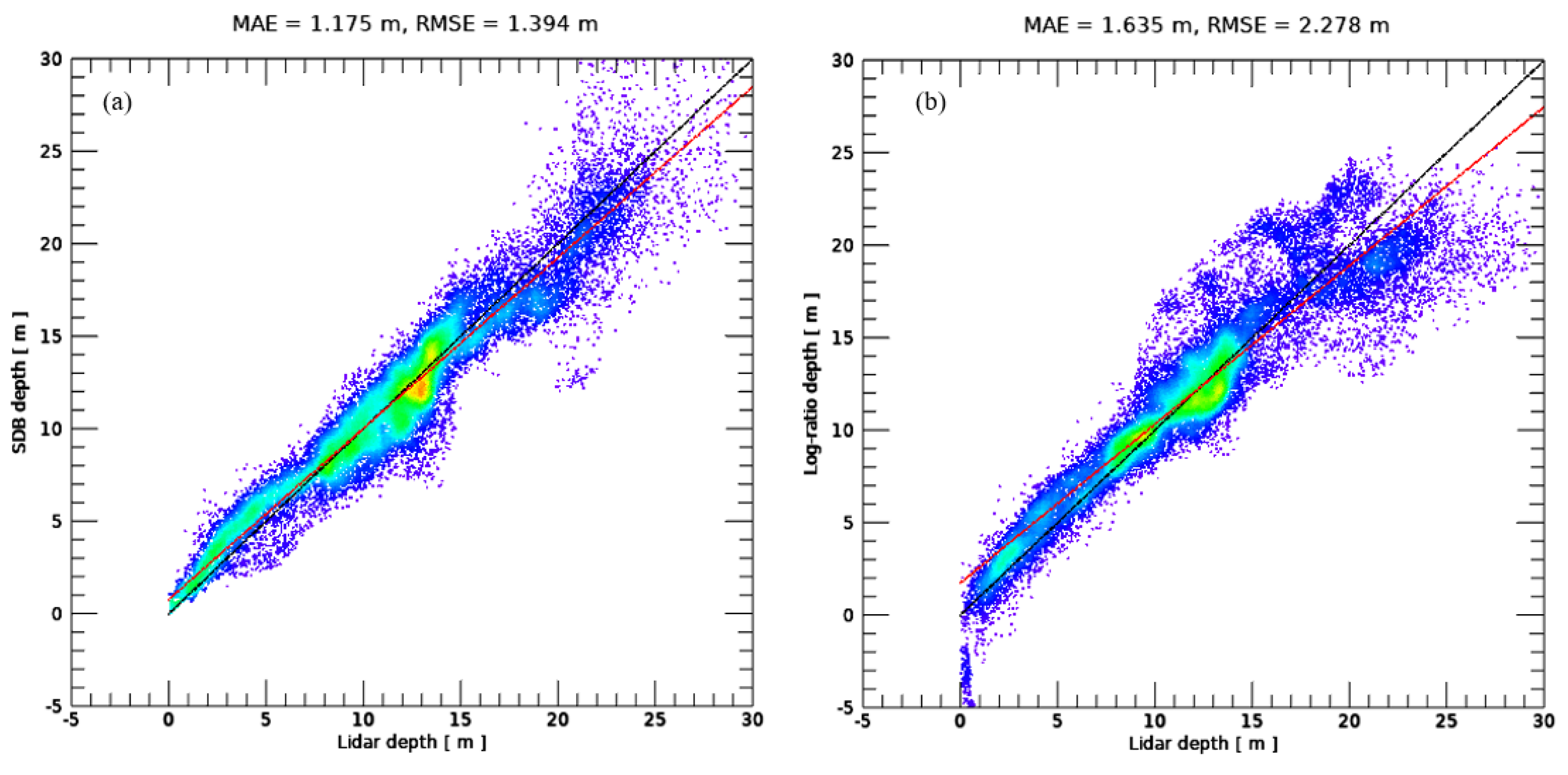
3.11. Comparison with Log-Ratio Method

Although comparing the performance of physics-based SDB to other methods is not the main interest of this paper, it may be beneficial to determine the improvements over other SDB methods. For instance, a commonly used method like Log-ratio by Stumpf [3] has a well-known key conceptual idea that the Log-ratio of the two bands may have a linear relationship with depth independently of bottom albedo. We use only the main concept without considering auxiliary tuning for the conditions specific to the Puerto Rico scene of this study (Figure 33a); thus, it is advised that the result may not be the best outcome from the Log-ratio method. After atmospheric correction, the green band to blue band log-ratio is linearly modeled against known lidar depth.

$$z=m_1·\frac{\ln {\rho }_{BOA}\left(Green\right)}{\ln {\rho }_{BOA}\left(Blue\right)}+m_0$$

(31)

The training data used for obtaining the linear regression coefficients $m_0$ and $m_1$ are 10% of the pixels in the bounding box. The Log-ratio of the entire scene is computed, and the regression coefficients are applied to obtain depths. The comparison between the physics-based depths, Log-ratio depth, and the lidar depth are shown in Figure 33b–d. Both algorithms produce depths that compare with the lidar depth quite well. The overall error analysis is shown in the depth scatterplot (Figure 34), where physics-based SDB shows improved MAE and RMSE compared to the Log-ratio method.

3.12. Discussion

The governing equation for the water-leaving reflectance over optically shallow water is an approximated equation, and it was derived based on two-flow radiative transfer theory [22,23,24]. Many shallow water inversion studies including SDB were published using the reflectance equation. The governing equation has several different forms depending on the types of the model variables, such as radiance or irradiance and surface or subsurface. When the Hydrolight numerical solution of ocean optical radiative transfer was created as a research tool by Mobley [25,26], many remote sensing reflectances were simulated over a wide range of incident radiance distributions, surface conditions, vertical profiles of optical properties, and bottom albedo. By analyzing many simulated reflectances, a governing equation in the form of subsurface remote sensing reflectance was suggested [27], which our suggested physics-based SDB algorithm also uses, as shown in Equation (19). The inherent optical property models for chlorophyll, dissolved organic matter, and suspended detritus and solids as described in Equations (5)–(9) are well established in the ocean optics community [28]. Atmospheric correction before applying semi-analytic algorithms may have slight differences, but the effect should be negligible in most optically shallow water compared to major sources of errors such as unknown bottom albedo. In our research, we used Ahmad RT LUT because 6SV and MODTRAN LUT lack the capability of handling the water surface reflected sky radiance component. Differences in numerical solution methods such as nonlinear optimization [19,27,29] or the look-up-table method [21,30,31,32] have negligible effects on the accuracy of the result and are simply a matter of choice.

Considering all the related components of the semi-analytic method, differences are not substantial between many different previous studies. One major difference in the inversion of the semi-analytic model is how to handle bottom albedo. Some methods assume only a single endmember bottom model, which is one generic sand-like or grass-like bottom type [27,33] that estimates the weights of the normalized bottom spectrum. The approach implies that the depth and other inversion results could be erroneous by design over the area with the other bottom type. In practice, a sand bottom is used if water-leaving reflectance is greater than tolerance; otherwise, a grass bottom is used [29]. A different strategy is to create many combinations using two bottom endmembers from the library and then iteratively optimize the system and choose a unique combination that results in minimum total error [34,35]. However, the assumption of known local bottom spectra is not practical in most cases.

Our approach is to use two endmembers with the linear unmixing concept. During optimization for SDB inversion, two unknown mixing coefficients are estimated along with the depth. The two most generic endmembers (sand-like and algae- or vegetation-like) give more freedom to apply SDB to an arbitrary coastal zone with a range of mixed bottoms of typical sand or grass. This means no a priori knowledge of site-specific bottom albedo. In most inland water or coastal water, aquatic vegetation or dark bottoms are covered with a thick coat of mud. In that case, it is justified to use a single mud- or sand-like bottom. Our suggested approach can be readily applied when no ground truth reference data (lidar or sonar) are available, although known depth information will improve the accuracy.

When lidar depths over a shallow water area are available, scene-derived bottom endmembers can be estimated. We used eigenanalysis and the detailed its successful application. We also provided several tuning strategies for when a small set of lidar depths are available.

Another emphasis we made was that all the procedures were tailored to be applicable to a small number of bands. So, even minimum three-band satellite imagery can be processed in cases when the simplification assumptions are viable. Many physics-based SDB algorithms operate on hyperspectral data that inherently require a large number of bands. They cannot be applied to typical multispectral satellite data with only three or four bands in the visible wavelength range.

We utilized generic optical theories and models and adopted the concept of generic mixing of two endmembers to enhance the applicability. Also, we made meaningful performance-enhancing strategies for multi-band SDB. As a result, our SDB system consistently produces up to 30 m depth over relatively clear water with about 1.0 m of MAE and 1–1.5 m of RMSE, which we believe is quite useful in the absence of lidar or sonar data.

A physics-based SDB algorithm solves for water depth from a radiometrically calibrated satellite coastal zone image using a sequence of physics theories, such as atmospheric theory, ocean bio-optics theory, and the radiative transfer of hydro-optics. All these base physics theories are expressed using many parameters that need to be obtained from the multi-band spectrum of the image via inversion solutions. Thus, the primary constraint of physics-based SDB is the number of bands of the satellite image. If larger numbers of bands are available, pixel-by-pixel solutions for many parameters are possible, which may produce better results. In the case of Landsat OLI, only four bands are available in the visible wavelengths. Thus, the atmospheric solution and water optical property solution are obtained from an optically deep region of the image, and then we have no other choice but to assume the same atmospheric condition and optical properties apply to the optically shallow region, too. In that case, the pixel-by-pixel SDB solution is just an optimization problem for three variables (depth and two bottom weights). Thus, the obvious limitation of this technique is that it can be applied only to areas of homogeneous atmosphere and water optical properties. However, it is only because of the limited number of bands, not because of the limited capability of physics-based SDB itself. Another limitation is the general applicability of bottom spectral albedo. A generic version of bottom spectra (sand-like and grass-like) may have some difference compared to a local specific bottom of a similar kind.

Future research endeavors include the following. The current approach finds a satellite image with the lowest cloud cover and the clearest water. If SDB is applied to multiple satellite images collected at several different times, it will be possible to fix the erroneous area by patching the erroneous area using a better-quality image collected at a different overpass time. The properties of a better-quality image are lesser cloud cover and clearer water. Another important improvement needed is the collection of bottom reflectance spectra from a wide range of coastal zones. An enhanced literature review of sea floor reflectance measurement campaigns will be greatly beneficial to add a bottom library from various global locations.

4. Conclusions

As the theory of SDB includes atmospheric radiative transfer and ocean optical radiative transfer modeling, the algorithm presented here is categorized as a physics-based method. Technical details of the physics-based SDB method starting from the satellite image to depth inversion were presented. The sampling of optically deep water for atmospheric correction and the estimation of optical properties was emphasized as a crucial step. The next step was to apply SDB over an optically shallow region. This two-step approach is necessary to solve a complex physical system with a much larger number of unknowns when only four bands of OLI in visible wavelengths are available. Regarding bottom reflectance, a method to estimate scene-derived bottom endmembers using eigenanalysis was presented. A technique to constrain all parameters to be physically valid in the solution process using Levenberg–Marquardt numerical optimization was also described.

The TBDEM was resampled for each satellite image pixel. Based on the pixel spectral characteristics, a DEM offset was estimated at the time of satellite overpass to convert the DEM to lidar water depth. The depth error was mostly about 1 m or less in terms of MAE and less than 2 m in terms of RMSE for a depth range of up to 30 m in the case of relatively clear water. For non-typical bottom types, the physics-based approach requires fine-tuning to fit to site-specific conditions. The fine-tuning consists of the modification of bottom reflectance or the diffuse attenuation coefficient.

Although this technique could be used without reference depths from lidar or sonar, known depths from other sources can be used for fine-tuning site-specific bottom endmembers. For instance, our physics-based SDB system is fine-tuned using an available bathymetric lidar DEM over the southwest corner of Puerto Rico; then, the depth map of the entire coastline of the island can be created using Landsat OLI images. Although the point density is very low, the ICESat-2 (ice, cloud and land elevation satellite) bathy point cloud is a globally available data source for fine-tuning.

References

1. Lyzenga, D.R. Passive remote sensing techniques for mapping water depth and bottom features. Appl. Opt. 1978, 17, 379–383. [Google Scholar] [CrossRef]
2. Lyzenga, D.; Malinas, N.; Tanis, F. Multispectral bathymetry using a simple physically based algorithm. IEEE Trans. Geosci. Remote Sens. 2006, 44, 2251–2259. [Google Scholar] [CrossRef]
3. Stumpf, R.P.; Holderied, K.; Sinclair, M. Determination of water depth with high-resolution satellite imagery over variable bottom types. Limnol. Oceanogr. 2003, 48, 547–556. [Google Scholar] [CrossRef]
4. Ashphaq, M.; Srivastava, P.K.; Mitra, D. Review of near-shore satellite derived bathymetry: Classification and account of five decades of coastal bathymetry research. J. Ocean Eng. Sci. 2021, 6, 340–359. [Google Scholar] [CrossRef]
5. USGS Earth Explorer. Available online: https://earthexplorer.usgs.gov/ (accessed on 20 January 2024).
6. USGS GloVis. Available online: https://glovis.usgs.gov/ (accessed on 20 January 2024).
7. LandsatLook Viewer. Available online: https://landsatlook.usgs.gov/ (accessed on 20 January 2024).
8. Berk, A.; Conforti, P.; Kennett, R.; Perkins, T.; Hawes, F.; van den Bosch, J. MODTRAN6: A major upgrade of the MODTRAN radiative transfer code. In SPIE 9088, Algorithms and Technologies for Multispectral, Hyperspectral, and Ultraspectral Imagery XX, 90880H (13 June 2014); SPIE: Bellingham, WA, USA, 2014. [Google Scholar] [CrossRef]
9. Berk, A.; Conforti, P.; Hawes, F. An accelerated line-by-line option for MODTRAN combining on-the-fly generation of line center absorption with 0.1 cm−1 bins and pre-computed line tails. In SPIE 9471, Algorithms and Technologies for Multispectral, Hyperspectral, and Ultraspectral Imagery XXI, 947217 (21 May 2015); SPIE: Bellingham, WA, USA, 2015. [Google Scholar] [CrossRef]
10. Kotchenova, S.Y.; Vermote, E.F.; Matarrese, R.; Klemm, E.F., Jr. Validation of a vector version of the 6S radiative transfer code for atmospheric correction of satellite data. Part I: Path Radiance. Appl. Opt. 2006, 45, 6726–6774. [Google Scholar] [CrossRef] [PubMed]
11. Kotchenova, S.Y.; Vermote, E.F. Validation of a vector version of the 6S radiative transfer code for atmospheric correction of satellite data. Part II: Homogeneous Lambertian and anisotropic surfaces. Appl. Opt. 2007, 46, 4455–4464. [Google Scholar] [CrossRef]
12. Ahmad, Z.; Fraser, R.S. An iterative radiative transfer code for ocean–atmosphere systems. J. Atmos. Sci. 1982, 39, 656–665. [Google Scholar] [CrossRef]
13. Gao, B.C.; Montes, M.J.; Ahmad, Z.; Davis, C.O. Atmospheric correction algorithm for hyperspectral remote sensing of ocean color from space. Appl. Opt. 2000, 39, 887–896. [Google Scholar] [CrossRef]
14. Montes, M.J.; Gao, B.C.; Davis, C.O. Atmospheric Correction Algorithms: Tafkaa User’s Guide, NRL/MR/7230—04-8760. Available online: https://apps.dtic.mil/sti/pdfs/ADA422084.pdf (accessed on 20 January 2024).
15. Lee, Z.-P. (Ed.) Remote Sensing of Inherent Optical Properties: Fundamentals, Tests of Algorithms, and Applications; Reports of the International Ocean-Colour Coordinating Group, No. 5; IOCCG: Dartmouth, NS, Canada, 2006. [Google Scholar]
16. Gordon, H.R.; Brown, O.B.; Evans, R.H.; Brown, J.W.; Smith, R.C.; Baker, K.S.; Clark, D.K. A semianalytic radiance model of ocean color. J. Geophys. Res. 1988, 93, 10909–10924. [Google Scholar] [CrossRef]
17. Mobley, C.D. Light and Water: Radiative Transfer in Natural Waters; Academic: San Diego, CA, USA, 1994. [Google Scholar]
18. Kim, M.; Park, J.Y.; Tuell, G. A Constrained Optimization Technique for Estimating Environmental Parameters from CZMIL Hyperspectral and Lidar Data, Hyperspectral and Ultraspectral Imagery XVI, 769513; SPIE: Bellingham, WA, USA, 2010. [Google Scholar] [CrossRef]
19. Donald, M. An algorithm for least-squares estimation of nonlinear parameters. SIAM J. Appl. Math. 1963, 11, 431–441. [Google Scholar]
20. Mobley, C.D.; Sundman, L.K.; Davis, C.O.; Bowles, J.H.; Downes, T.V.; Leathers, R.A.; Montes, M.J.; Bissett, W.P.; Kohler, D.D.R.; Reid, R.P.; et al. Interpretation of hyperspectral remote-sensing imagery by spectrum matching and look-up tables. Appl. Opt. 2005, 4, 3576–3592. [Google Scholar] [CrossRef]
21. International Hydrographic Organization IHO. S-44 IHO Standards for Hydrographic Surveys Edition 6.1.0; International Hydrographic Organization: Monaca, France, 2022; Available online: https://iho.int/uploads/user/pubs/standards/s-44/S-44_Edition_6.1.0.pdf (accessed on 20 January 2024).
22. Philpot, W.D. Bathymetric Mapping with Passive Multispectral Imagery. Appl. Opt. 1989, 28, 1569–1578. [Google Scholar] [CrossRef]
23. Maritorena, S.; Morel, A.; Gentili, B. Diffuse reflectance of oceanic shallow waters: Influence of water depth and bottom albedo. Limnol. Oceanogr. 1994, 39, 1689–1703. [Google Scholar] [CrossRef]
24. Morel, A.; Maritorena, S. Bio-optical properties of oceanic waters: A reappraisal. J. Geophys. Res. Ocean. 2001, 106, 7163–7180. [Google Scholar] [CrossRef]
25. Mobley, C.D. Estimation of the remote-sensing reflectance from above-surface measurements. Appl. Opt. 1999, 38, 7442–7445. [Google Scholar] [CrossRef] [PubMed]
26. Mobley, C.D.; Sundman, L.K. Hydrolight 5 Ecolight 5 Technical Documentation; Sequoia Scientific, Inc.: Bellevue, WA, USA, 2008; p. 100. [Google Scholar]
27. Lee, Z.; Carder, K.L.; Mobley, C.D.; Steward, R.G.; Patch, J.S. Hyperspectral remote sensing for shallow waters. 2. Deriving bottom depths and water properties by optimization. Appl. Opt. 1999, 38, 3831–3843. [Google Scholar] [CrossRef] [PubMed]
28. Sathyendranath, S. (Ed.) Remote Sensing of Ocean Colour in Coastal, and Other Optically-Complex, Waters; Reports of the International Ocean-Colour Coordinating Group, No. 3; IOCCG: Dartmouth, NS, Canada, 2000. [Google Scholar]
29. Huang, R.; Yu, K.; Wang, Y.; Wang, J.; Mu, L.; Wang, W. Bathymetry of the coral reefs of Weizhou Island based on multispectral satellite images. Remote Sens. 2017, 9, 750. [Google Scholar] [CrossRef]
30. Garcia, R.A.; Lee, Z.; Hochberg, E.J. Hyperspectral shallow-water remote sensing with an enhanced benthic classifier. Remote Sens. 2018, 10, 147. [Google Scholar] [CrossRef]
31. Wang, Y.; He, X.; Bai, Y.; Li, T.; Wang, D.; Zhu, Q.; Gong, F. Satellite-Derived Bottom Depth for Optically Shallow Waters Based on Hydrolight Simulations. Remote Sens. 2022, 14, 4590. [Google Scholar] [CrossRef]
32. Hedley, J.D.; Roelfsema, C.; Phinn, S.R. Efficient radiative transfer model inversion for remote sensing applications. Remote Sens. Environ. 2009, 113, 2527–2532. [Google Scholar] [CrossRef]
33. Eugenio, F.; Martin, J.; Marcello, J.; Fraile-Nuez, E. Environmental monitoring of El Hierro Island submarine volcano, by combining low and high resolution satellite imagery. Int. J. Appl. Earth Obs. Geoinform. 2014, 29, 53–66. [Google Scholar] [CrossRef]
34. Klonowski, W.M.; Fearns, P.R.; Lynch, M.J. Retrieving key benthic cover types and bathymetry from hyperspectral imagery. J. Appl. Remote Sens. 2007, 1, 011505. [Google Scholar] [CrossRef]
35. Brando, V.E.; Anstee, J.M.; Wettle, M.; Dekker, A.G.; Phinn, S.R.; Roelfsema, C. A physics-based retrieval and quality assessment of bathymetry from suboptimal hyperspectral data. Remote Sens. Environ. 2009, 113, 755–770. [Google Scholar] [CrossRef]
Figure 1. Diagram of a water surface reflected sky radiance (blue arrow) and intrinsic atmospheric volume backscattered reflectance (black arrow).
Remotesensing 16 00843 g001
Figure 2. Example IOP measurements from various optical conditions: (a) absorption spectra due to detritus and gelbstoff; (b) backward scattering spectra due to suspended particulates.
Remotesensing 16 00843 g002
Figure 3. Simulated reflectance of optically shallow water over varying depths (0.2, 1, 2, 4, 6, 12 m). The cyan-colored curves represent the first term of Equation (19), where the depths increase from the bottom to the top curves. The yellow-colored curves represent the second term of Equation (19), where the depths increase from the top to the bottom curves. The black-colored curves are the sum of the two terms, where the depths increase from the top to the bottom curves.
Remotesensing 16 00843 g003
Figure 4. Bottom spectral library with selected example of sand bottom in yellow and grass bottom in green collected at Lee Stocking Island, Bahamas [20]. The yellow and green curves are the initially selected bottom library for SDB.
Remotesensing 16 00843 g004
Figure 5. (a) An example Landsat 8 OLI scene, southwest corner of Puerto Rico. (b) Optically deep-water spectrum sampled from the yellow cross. The mean TOA reflectance ρ T O A from the yellow cross-marked optically deep area is shown as a yellow curve. After atmospheric correction, the surface reflectance ρ B O A is shown as a gray curve. For an optimized τ a , the dotted gray curve is the ρ B O A result using 6SV LUT [10], and the solid gray curve is the ρ B O A result using Ahmad LUT [12]. In similar manner, the red-colored curves represent above-surface remote sensing reflectance, and the cyan-colored curves represent subsurface remote sensing reflectance.
Remotesensing 16 00843 g005
Figure 6. Atmospheric correction. (a) 6SV LUT [10], (b) Ahmad LUT [12], (c) reflectance, and (d) transmission. For (a,b), the gray curve is TOA reflectance, the blue curve is the reflectance due to Rayleigh scattering, the yellow curve is the reflectance due to aerosol, and the cyan curve is combined atmospheric reflectance. The cyan curve in (b) by Ahmad LUT includes water surface reflection component; that is why the spectrum is higher than 6SV LUT. The magenta curve is the ρ s component in Equation (2), and the green curve is the final ρ B O A . For (c), a set of solid lines are using Ahmad LUT and a ser of dashed lines are using 6SV LUT. The gray curves are ρ B O A , the red curves are the water-leaving reflectances, and the cyan curves are the subsurface remote sensing reflectances. For (d), the green curve is T o z , the magenta curve is T o g T w v , and the gray curve represents t s τ a t v τ a .
Remotesensing 16 00843 g006
Figure 7. Analysis of optically deep water. (a) Subsurface remote sensing reflectance analysis. (b) Analysis of inherent optical properties after optimization. The curves in (a) are described in Figure 6c. The subsurface remote sensing r r s , which is the cyan-colored curve in (a), is converted to u , which is the thick gray dot in (b). The optimized result is the cyan curve in (b). The phytoplankton absorption is the dotted green line, detritus and gelbstoff absorption are the dotted yellow lines, total absorption including pure water is the dashed red line, particulate backward scattering is the dotted gray line, total backward scattering including pure water is the dashed red line, and K u ,   K d —using Equations (17) and (18)—are the solid gray and solid yellow lines, where the solar zenith angle of the pixel location is SZA = 44.9° and VZA = 3.1°. Frequently used variables K u ,   K d at 532 nm are also marked, which is the case of typical relatively clear coastal water.
Remotesensing 16 00843 g007
Figure 8. Simulated reflectance spectra (a) for varying depths, (b) for varying attenuation coefficients K with increment of 0.01 at 3 depths, and (c) for all bottom library spectra at 3 depths. For (b,c), gray lines are 2 m, green lines are 5 m, and red lines are 15 m depth.
Remotesensing 16 00843 g008
Figure 9. SDB area of interest in Puerto Rico. (a) Satellite image. (b) Bathymetric lidar point cloud in grayscale.
Remotesensing 16 00843 g009
Figure 10. Initial depth scatterplot between lidar water depth and SDB depth. The color of the dots represents the local density in the depth scatterplot: a rainbow color scheme with high density toward red and low density toward purple. The black line represents the one-to-one line, and the red line is the linear regression line.
Remotesensing 16 00843 g010
Figure 11. Estimation of DEM offset to convert to lidar DEM water depth. (a) Lidar DEM overlaid to satellite image in Key West. (b) Estimated water surface level in red line using land–water interface derived from satellite image, where green diamonds have spectral properties of water.
Remotesensing 16 00843 g011
Figure 12. Scene-derived bottom reflectance for Puerto Rico. (a) SDB scene. (b) Shallow water sampling area for scene-derived bottom reflectance. The sampling depth ranges are displayed in white pixels (0–0.5 m), green pixels (0.5–1.0 m), red pixels (1.0–1.5 m), and yellow pixels (1.5–2.0 m).
Remotesensing 16 00843 g012
Figure 13. Scene-derived bottom reflectance analysis. (a) Inverted bottom spectra. (b) Endmembers projected to a two-dimensional plot. In (a), the dashed green curve is ρ b g , the dashed yellow curve is ρ b s , and the dashed red line is the mean spectrum. In (b), the blue dots represent the distribution of ρ b that is projected to two dimensions: band 1 (coastal aerosol) on the x-axis and band 2 (blue) on the y-axis. The green diamond along the regression line of the blue points corresponds to the k s value, and the yellow diamond corresponds to k g . The green dots represent the projection to two dimensions: band 2 (blue) on the x-axis and band 3 (green) on the y-axis. The red dots represent the projection to two dimensions: band 3 (green) on the x-axis and band 4 (red) on the y-axis. The bottom reflectance is dimensionless.
Remotesensing 16 00843 g013
Figure 14. Depth scatterplot between lidar DEM versus SDB depth after using scene-derived endmember bottom library.
Remotesensing 16 00843 g014
Figure 15. Three-dimensional visualization of bathymetry for Puerto Rico. (a) SDB. (b) Bathymetric lidar DEM.
Remotesensing 16 00843 g015
Figure 16. Sampling location of pixels and SDB optimization results. (a) Blue-dot pixel, very shallow—less than 1 m water. (b) Yellow-dot pixel—about 2 m depth near Puerto Rico. (c) Red-dot pixel—about 15 m depth. (d) Green-dot pixel—about 20 m depth. The diamond dots are the r r s 4-band spectrum from the OLI scene. The gray curve is the optimized model r r s . The yellow curve represents ( ρ b s / π ) · exp   K u + K d · z , the green curve represents ( ρ b g / π ) · exp   K u + K d · z , and the red curve is the sum of the two. The cyan curve represents the water volume backscattered subsurface reflectance r r s , · 1 exp   K u + K d · z , which is the first term in Equation (19). All four figures show the fraction of sand-like and grass-like bottom fraction, optimized SDB depth, and the corresponding bathymetric lidar DEM depth.
Remotesensing 16 00843 g016
Figure 17. Comparison between SDB and DEM along transect lines near Puerto Rico. (a) Location of transect lines. (b) Depth profiles along the yellow line. (c) Depth profiles along the green line. (d) Depth profiles along the red line. Green dots are lidar-derived water depth, while white dots are SDB water depth.
Remotesensing 16 00843 g017
Figure 18. SDB example at Puerto Rico. (a) Image, (b) DEM, and (c) depth scatterplot.
Remotesensing 16 00843 g018
Figure 19. SDB example of Puerto Rico. (a) Image, (b) error scatterplot, (c) 3D visualization of SDB depth, and (d) 3D visualization of lidar depth.
Remotesensing 16 00843 g019
Figure 20. SDB example for Key West. (a) Satellite image. (b) Bathymetric lidar DEM drawn over the image.
Remotesensing 16 00843 g020
Figure 21. Analysis of inherent optical properties after optimization from Key West.
Remotesensing 16 00843 g021
Figure 22. SDB results from Key West. (a) OLI image. (b) Lidar DEM overlaid in grayscale image. (c) Depth scatterplot.
Remotesensing 16 00843 g022
Figure 23. SDB example for Guam. (a) Satellite image. (b) Bathymetric lidar DEM drawn over the image. The yellow cross in (a) is the optically deep water where a pixel spectrum is sampled for atmospheric correction and IOP estimation.
Remotesensing 16 00843 g023
Figure 24. Analysis of inherent optical properties after optimization from Guam.
Remotesensing 16 00843 g024
Figure 25. SDB results from Guam. (a) Depth scatterplot, (b) 3D visualization of SDB result, and (c) 3D visualization of bathymetric lidar.
Remotesensing 16 00843 g025
Figure 26. Analysis of erroneous SDB from Guam. (a) The black-colored polygon of the erroneous region in the scatterplot. (b) Red pixels corresponding to the sampled pixel points in the polygon.
Remotesensing 16 00843 g026
Figure 27. SDB of Guam with fine-tuning. (a) Satellite image and SDB extent box, (b) bathymetric lidar DEM drawn over the image, and (c) depth scatterplot.
Remotesensing 16 00843 g027
Figure 28. Visualization of Guam in 3D after fine-tuning. (a) SDB in 3D. (b) TBDEM in 3D.
Remotesensing 16 00843 g028
Figure 29. Fine-tuning strategy. (a) Bottom reflectance scaling. (b) Adjustment of diffuse attenuation spectrum. The blue ellipse represents the depth points. Initial scatterplot ellipse in (a) can be vertically shifted to the direction of red arrow by scaling bottom reflectance ρ b . Initial scatterplot ellipse in (b) can be tilted to the direction of the red arrow by changing the attenuation spectrum K .
Remotesensing 16 00843 g029
Figure 30. Effect of diffuse attenuation coefficient. (a) SDB inversion area, (b) depth scatterplot using the diffuse attenuation obtained from the optically deep water of the scene, (c) depth scatterplot using lower diffuse attenuation, and (d) depth scatterplot using higher diffuse attenuation.
Remotesensing 16 00843 g030
Figure 31. Uncertainty of physics-based SDB in reference to IHO standards.
Remotesensing 16 00843 g031
Figure 32. SDB of the entire local region in Puerto Rico after fine-tuning using partially available TBDEM. The known TBDEM area is marked as a red-colored boundary.
Remotesensing 16 00843 g032
Figure 33. Depth profile along transect lines. (a) The Puerto Rico scene, comparing physics-based SDB and the Log-ratio method. The three transect lines in yellow (b), green (c), and red (d) colors are shown. The corresponding depth profiles are in diamond symbols, where physics-based SDB depth is in white, Log-ratio SDB depth is in red, and the lidar depth is in green.
Remotesensing 16 00843 g033
Figure 34. Depth scatterplot. (a) Physics-based SDB method. (b) Log-ratio SDB method.
Remotesensing 16 00843 g034