
Sea Ice Extraction via Remote Sensing Imagery: Algorithms, Datasets, Applications and Challenges

Abstract
:1. Introduction
2. Method of Sea Ice Extraction
2.1. Conventional Image Classification Methods
2.1.1. Bayesian
2.1.2. Maximum Likelihood Estimation
2.1.3. Thresholding Method
2.1.4. Other Statistical Approaches
2.1.5. Limitations
2.2. Machine Learning-Based Methods
2.2.1. Iterative Region Growing Using Semantics (IRGS)
2.2.2. Random Forest (RF)
2.2.3. Multilayer Perceptron (MLP)
2.2.4. Support Vector Machine (SVM)
2.2.5. Others
2.2.6. Limitations
2.3. Deep-Learning-Based Methods
2.3.1. Supervised Learning
2.3.2. Semi-Supervised Learning (SSL)
2.3.3. Unsupervised Learning
2.3.4. Limitations
3. Accessible Ice Datasets
3.1. SAR-Based Datasets
3.1.1. Radiation Characteristics of Sea Ice
- Radar wavelength Much of the literature on sea ice classification has discussed the effectiveness of different radar wavelengths, including the Ku-band, X-band, L-band and C-band SAR. In summary, the X-band and Ku-band are suitable for winter sea ice monitoring, while the L-band offers advantages for summer sea ice monitoring. The C-band, which lies between the Ku-band and L-band, provides a balanced choice for sea ice monitoring across different seasons. Currently, many sea ice monitoring tasks opt for SAR in the C-band for research purposes. The authors of [150] demonstrate that, compared to the C-band, the L-band is more accurate in detecting newly formed ice.
- Polarization mode Polarimetric techniques offer valuable insights into sea ice identification by capturing more detailed surface information using polarimetric SAR. This leads to improved classification of different sea-ice-types. For instance, the distinctive rough or deformed surfaces of FYI result in higher backscattering coefficients in cross-polarization. Conversely, MYI, known for its stronger volume scattering, exhibits higher backscattering coefficients in both co-polarization and cross-polarization. Notably, Nilas ice, characterized by its smooth surface and high salinity content, demonstrates consistently low backscattering coefficients across both polarizations in radar observations.
- Incidence angle In many scattering experiments, the statistical characteristics of sea ice backscattering coefficients with respect to varying incidence angles can be observed distinctly. When a radar emits microwaves towards a calm open water surface, the echo signal becomes prominent when the incidence angle is close to vertical or extremely small. However, as the incidence angle increases, the backscattering from the sea surface weakens, resulting in a gradual reduction in surface roughness. Research has shown that at higher frequency bands, increasing the incidence angle improves the classification accuracy between sea ice and open water. Additionally, the backscattering coefficients during the melting period of sea ice are also influenced by the incidence angle. For instance, in HH-polarized data, the backscattering coefficients obtained at small incidence angles are significantly higher, and they exhibit a linear relationship with increasing incidence angles.
3.1.2. Datasets
- SI-STSAR-7 [83] The dataset is a spatiotemporal collection of SAR imagery specifically designed for sea ice classification. It encompasses 80 Sentinel-1 A/B SAR scenes captured over two freeze-up periods in Hudson Bay, spanning from October 2019 to May 2020 and from October 2020 to April 2021. The dataset includes a diverse range of ice categories. The labels for the sea ice classes are derived from weekly regional ice charts provided by the Canadian Ice Service. Each data sample represents a 32 × 32 pixel patch of SAR imagery with dual-polarization (HH and HV) SAR data. These patches are derived from a sequence of six consecutive SAR scenes, providing a temporal dimension to the dataset.
- The TenGeoP-SARwv dataset [15] The dataset is built upon the acquisition of Sentinel-1A wave mode (WV) data in VV polarization. It comprises over 37,000 SAR image patches, which are categorized into 10 defined geophysical classes.
- SAR WV Semantic Segmentation The dataset is a subset of The TenGeoP-SARwv dataset. It consists of three parts: training, validation and testing. The images comprise 1200 samples and are stored as PNG format files with dimensions of 512 × 512 × 1 uint8. The label data are stored as npy files, represented by arrays of size 64 × 64 × 10, where each channel represents 1 of the 10 meteorological classes.
- KoVMrMl The dataset utilizes Sentinel-1 Interferometric Wide (IW) SAR data, including Single-Look Complex (SLC) and Ground Range Detected High-Resolution (GRDH) products in the HH channel. The GRDH images are annotated with 7 types of sea ice in patches of size 256 × 256. The H/ labeling is obtained by processing the dual-polarization SLC data using SNAP v9.0.0 software.
- SAR-based Ice types/lce edge dataset for deep learning analysis The dataset is specifically compiled for sea ice analysis in the northern region of the Svalbard archipelago, utilizing annotated polygons as references. It encompasses a total of 31 scenes and contains 6 distinct classes. The dataset is organized into data records, referred to as patches, which are extracted from the interior of each polygon using a stride of 10 pixels. Each class is represented by patches of different sizes, including 10 × 10, 20 × 20, 32 × 32, 36 × 36 and 46 × 46 pixels.
- AI4SeaIce [117] The dataset consists of 461 Sentinel-1 SAR scenes matched with ice charts produced by the Danish Meteorological Institute during the period of 2018–2019. The ice charts provide information on SIC, development stage and ice form in the form of manually drawn polygons. The dataset also includes measurements from the AMSR2 microwave radiomete sensor to supplement the learning of SIC, although the resolution is much lower than the Sentinel-1 data. Building upon the AI4SeaIce dataset, Song et al. [119] constructed an ice–water semantic segmentation dataset.
- Arctic sea ice cover product based on SAR [116] The dataset is based on Sentinel-1 SAR and provides Arctic sea ice coverage data. Approximately 2500 SAR scenes per month are available for the Arctic region. Each S1 SAR image acquired in the Arctic has been processed to generate NetCDF sea ice coverage data. Each S1 image corresponds to an NC file. The spatial resolution of the SAR-derived sea ice cover is 400 m. The website has released the processing of S1 data obtained in the Arctic from 2019 to 2021 and has uploaded the corresponding sea ice coverage data.
3.2. Optical-Based Datasets
3.2.1. Common Optical Sensors
- MODIS MODIS is an optical sensor widely used for ice classification. It is carried on the Terra and Aqua satellites. By observing the reflectance and emitted radiation of the Earth’s surface, MODIS can provide valuable information about ice characteristics such as color, texture and spectral properties.
- VIIRS VIIRS is an optical sensor with multispectral observation capabilities, used for monitoring and classifying the Earth’s surface. It provides high-resolution imagery and has applications in ice classification.
- Landsat series The Landsat satellites carry sensors that provide multispectral imagery for land cover classification and monitoring, including ice classification. Sensors such as OLI (Operational Land Imager) and TIRS (Thermal Infrared Sensor) on Landsat 8, as well as previous sensors like ETM+ (Enhanced Thematic Mapper Plus), have been extensively used in ice classification tasks.
- Sentinel series The European Space Agency’s Sentinel satellite series includes a range of sensors for Earth observation, including multispectral and thermal infrared sensors. The multispectral sensor on Sentinel-2 is utilized for ice classification and monitoring, while the sensors on Sentinel-3 provide information such as ice surface temperature and color.
- HY-1 (Haiyang-1) HY-1 also contribute to ice classification and monitoring. The HY-1 satellite is a Chinese satellite mission dedicated to oceanographic observations, including the monitoring of sea ice. The HY-1 satellite carries the SCA (Scanning Multichannel Microwave Radiometer) sensor, which operates in the microwave frequency range. This sensor can provide measurements of SIC, sea surface temperature and other related parameters. By detecting the microwave emissions from the Earth’s surface, the SCA sensor can differentiate between open water and ice.
- The VIIRS-based river ice maps [151] The dataset furnishes daily updates on river ice conditions across continental scales, encompassing the northern basins of the United States and the entirety of Canadian territory. Segmentation of VIIRS imagery holds promise for facilitating the detection and mapping of river ice, while also enabling the generation of additional classes such as snow, water and clouds.
3.2.2. Datasets
- 2021Gaofen Challenge The dataset is based on HY-1 visible light images with a resolution of 50 m. The scenes cover the surrounding region of the Bohai Sea in China. The provided images have varying sizes ranging from 512 to 2048 pixels and consist of over 2500 images. Each image has been manually annotated at the pixel level for sea ice, resulting in two classes: sea ice and background. The remote-sensing images are stored in TIFF format and contain the R-G-B channels, while the annotation files are in PNG format with a single channel. In the annotation files, sea ice pixels are assigned a value of 255, and background pixels have a value of 0.
- Arctic Sea Ice Image Masking The dataset consists of 3392 satellite images of the Hudson Bay sea ice in the Canadian Arctic region, captured between 1 January 2016 and 31 July 2018. The images are acquired from the Sentinel-2 satellite and composed of bands 3, 4 and 8 (false color). Each image is accompanied by a corresponding mask that indicates the SIC across the entire image.
3.3. Datasets Based on Alternative Acquisition Methods
- Airborne camera-based datasets The dataset is constructed from GoPro images captured during a two-month expedition conducted by the Nathaniel B. Palmer icebreaker in the Ross Sea, Antarctica [130]. The video clips captured can be found at https://youtu.be/BNZu1uxNvlo, accessed on 1 January 2024. These images were manually annotated using the open-source annotation tool PixelAnnotationTool into four categories: ice, ship, ocean and sky. The dataset was divided into three sets, namely training, validation and testing, in an 8:1:1 ratio. Data augmentation was performed by horizontally flipping the images, resulting in a training dataset of 382 images.
- River ice segmentation [152] The dataset collects digital images and videos captured by drones during the winter seasons of 2016–2017 from two rivers in Alberta province: the North Saskatchewan River and the Peace River. The images in the dataset are segmented into three categories: ice, anchor ice and water. The training set consists of 50 pairs, while the validation set includes 104 images; however, there are no labels available for the validation set.
- NWPU_YRCC2 dataset A total of 305 representative images were selected from videos and images captured by drones during aerial surveys of the Yellow River’s Ningxia-Inner Mongolia section. These images contain 4 target classes and were cropped to a size of 1600 × 640 pixels. The majority of these images were collected during the freezing period. Each pixel of the images was labeled into one of four categories: coastal ice, drifting ice, water and other using Adobe Photoshop 2020 software. The dataset was split into training, validation and testing sets in a ratio of 6:2:2, comprising 183, 61 and 61 images, respectively.

| Type | Dataset | Data Source | Research Area | Task | Ref. | Download Link (accessed on 1 January 2024) |
|---|---|---|---|---|---|---|
| SAR-based | SI-STSAR-7 | Sentinel-1 A/B dual-polarization (HH and HV) in EW scan mode | cover the entire open ocean | Classified by: OW, NI, GI, GWI, ThinFI, MedFI and ThickFI | [83] | http://ieee-dataport.org/open-access/si-stsar-7 |
| The TenGeoP-SARwv dataset | the WV in VV polarization from Sentinel-1A | over the open ocean | Classified by: Atmospheric Fronts, Biological Slicks, Icebergs, Low Wind Area, Micro Convective Cells, Oceanic Fronts, Pure Ocean Waves, Rain Cells, Sea Ice, Wind Streaks | [15] | https://www.seanoe.org/data/00456/56796/ | |
| SAR_WV Semantic Segmentation | Same as above | Same as above | Same as above | [125] | https://www.kaggle.com/datasets/rignak/sar-wv-semanticsegmentation | |
| KoVMrMl | Sentinel-1 IW SAR data, including SLC and GRDH products with HH channel | Belgica Bank, an ice-covered area along the north-east coast of Greenland | Classified by: Water, Young ice, FYI, Old ice, Mountains, Iceberg, Glaciers and Floating Ice | [147] | https://drive.google.com/file/d/1VK2geghwl_JUuEETntG_3_5rDBH8qnHN/view?usp=sharing | |
| SAR based Ice types/lce edge dataset for deep learning analysis | Sentinel-1A EW GRDM | north of Svalbard | Classified by: Open Water, Leads with Water, Brash/Pancake Ice, Thin Ice, Thick Ice-Flat and Thick Ice-Ridged | — | https://dataverse.no/dataset.xhtml?persistentId=doi:10.18710/QAYI4O | |
| AI4SeaIce | The Sentinel-1 dual-polarization HH and HV, along with the PMR measurements from the AMSR2 instrument on the JAXA GCOM-W satellite | the waters surrounding Greenland | Sea ice concentration, developmental stages, and forms of sea ice | [117] | https://data.dtu.dk/articles/dataset/AI4Arctic_ASIP_Sea_Ice_Dataset_-_version_2/13011134/2 | |
| Arctic sea ice cover product based on spaceborne SAR | Sentinel-1 dual-polarization HH/HV data in EW mode | the Arctic | Arctic sea ice coverage data | [116] | https://www.scidb.cn/en/detail?dataSetId=771301999089025024 | |
| Optical-based | 2021Gaofen Challenge | HY-1 visible light imagery with a resolution of 50 m | near the Bering Strait, China | Segmentation into sea ice and background | [9] | https://www.gaofen-challenge.com/challenge/competition/2 |
| Arctic Sea Ice Image Masking | The Sentinel-2 satellite, composed of bands 3, 4, and 8 (false-color) | Hudson Bay sea ice in the Canadian Arctic | Segmented into different SIC categories | https://www.kaggle.com/datasets/alexandersylvester/arctic-sea-ice-image-masking | ||
| The VIIRS-based river ice maps | The following VIIRS I-bands are used: I01, I02, I03, and I05 | all rivers and waterbodies from western Alaska to the east coast of the US and Canada | Segmented into water, land, vegetation, snow, river ice, cloud, and cloud shadow | [151] | https://web.stevens.edu/ismart/land_products/rivericemapping.html | |
| Airborne camera-based | Sea Ice Detection Dataset and Sea Ice Classification Dataset | GoPro images captured by the Nathaniel B. Palmer icebreaker | Ross Sea, Antarctica | automated detection of sea ice (ice, ocean, vessel, and sky) and classifying sea-ice-types (ocean, vessel, sky, lens artifacts, FYI, new ice, grey ice, and MYI) | [130] | https://youtu.be/BNZu1uxNvlo |
| Drone-based | River ice segmentation | The Reconyx PC800 Hyperfire professional game camera, and the Blade Chroma drone equipped with the CGO3 4K camera at the Genesee dock | two Alberta rivers: North Saskatchewan River and Peace River | Segmented into ice, anchor ice, and water | [152] | https://ieee-dataport.org/open-access/alberta-river-ice-segmentation-dataset |
| NWPU_YRCC2 dataset | a fixed wing UAV ASN216 with a Canon 5DS visible light camera and a DJI Inspire 1 | the Ningxia–Inner Mongolia reach of the Yellow River | Segmented into: coastal ice, pack ice, water, and other | [16] | https://github.com/nwpulab113/NWPUYRCC2 |
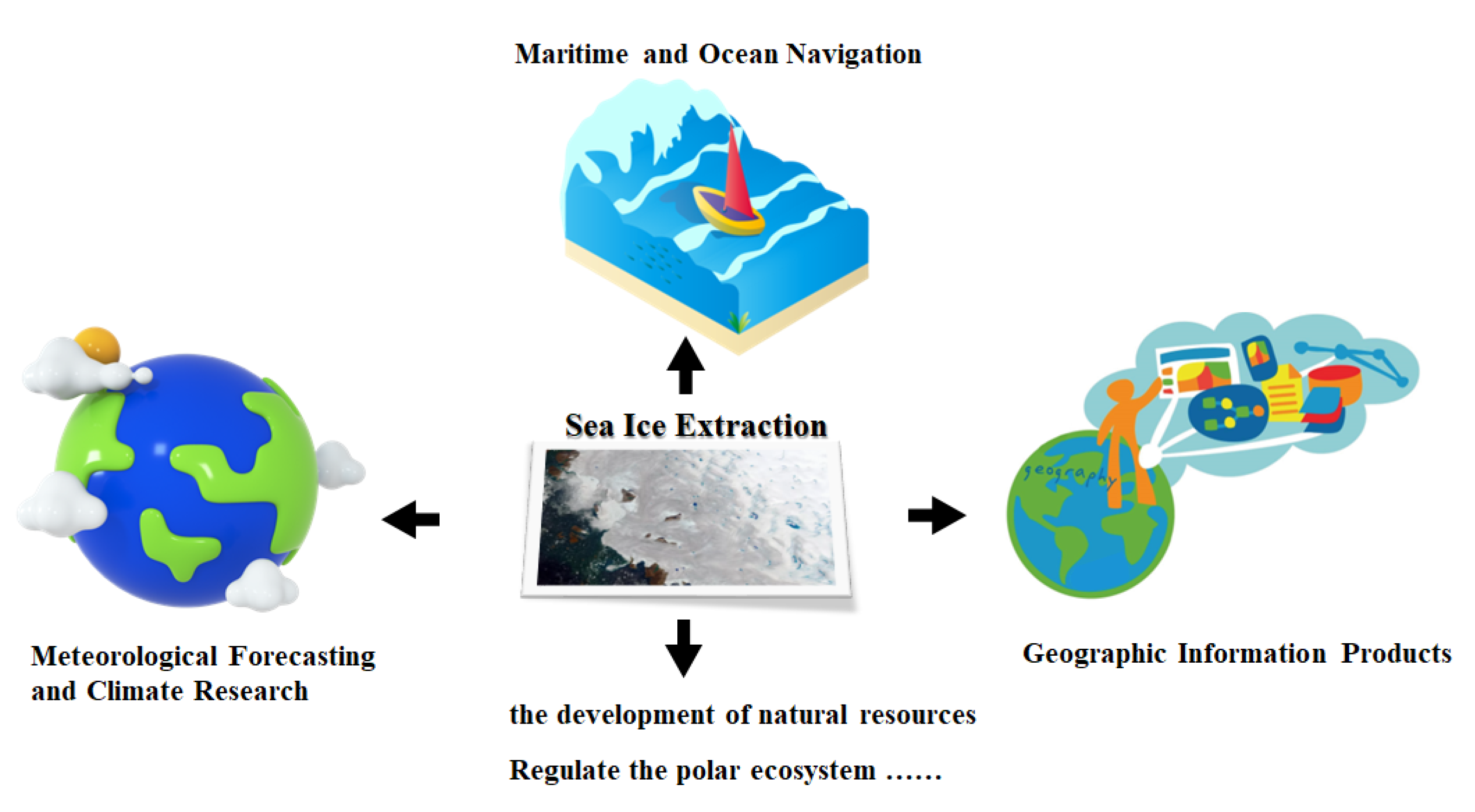
4. Applications
4.1. Meteorological Forecasting and Climate Research
4.2. Maritime and Ocean Navigation
4.3. Geographic Information Products
4.4. Others
5. Challenges in Sea Ice Detection
5.1. Exploration Methods Aspect
5.1.1. Multi-Sensor Integration
5.1.2. Underwater Ice Detection
5.2. Model Approaches Aspect
5.2.1. Multi-Source Data Fusion Model
5.2.2. Unsupervised Deep Learning
5.2.3. Construct ICE-SAM Large Model
5.3. Cartographic Applications Aspect
5.3.1. Polar Geographic Information Systems (GIS)
- Data Integration and Management. Polar systems should integrate sea ice data from multiple sources and manage them in a unified and standardized manner. This includes satellite observations, marine measurements and more. To enable structured modeling and geospatial analysis, the data integration and management module should incorporate functionalities such as data cleansing, format conversion, quality control and metadata management.
- Structured Modeling. The system needs to develop algorithms and models for structured modeling of sea ice, transforming raw sea ice data into structured representations with geospatial information. This involves modeling sea ice morphology, density, thickness, distribution and the relationships between sea ice and other geographical features. The sea ice structured modeling module should consider the spatiotemporal characteristics of sea ice and establish associations with the geographic coordinate system.
- Geospatial Analysis Capabilities. The system should provide a wide range of geospatial analysis functions to extract useful geospatial information from the sea ice structured model. This may include spatiotemporal analysis of sea ice changes, thermodynamic property analysis, analysis of sea ice interactions with the marine environment and more. The geospatial analysis module should support various analysis methods and algorithms, along with interactive visualization and result presentation.
- Real-time Data and Updates. To ensure timeliness, the system should support real-time acquisition and updates of sea ice data. This can be achieved through real-time connections with data sources such as satellite observations, buoys, UAVs and more. Additionally, the system should possess efficient and scalable data storage and processing capabilities to handle large-scale data-processing requirements.
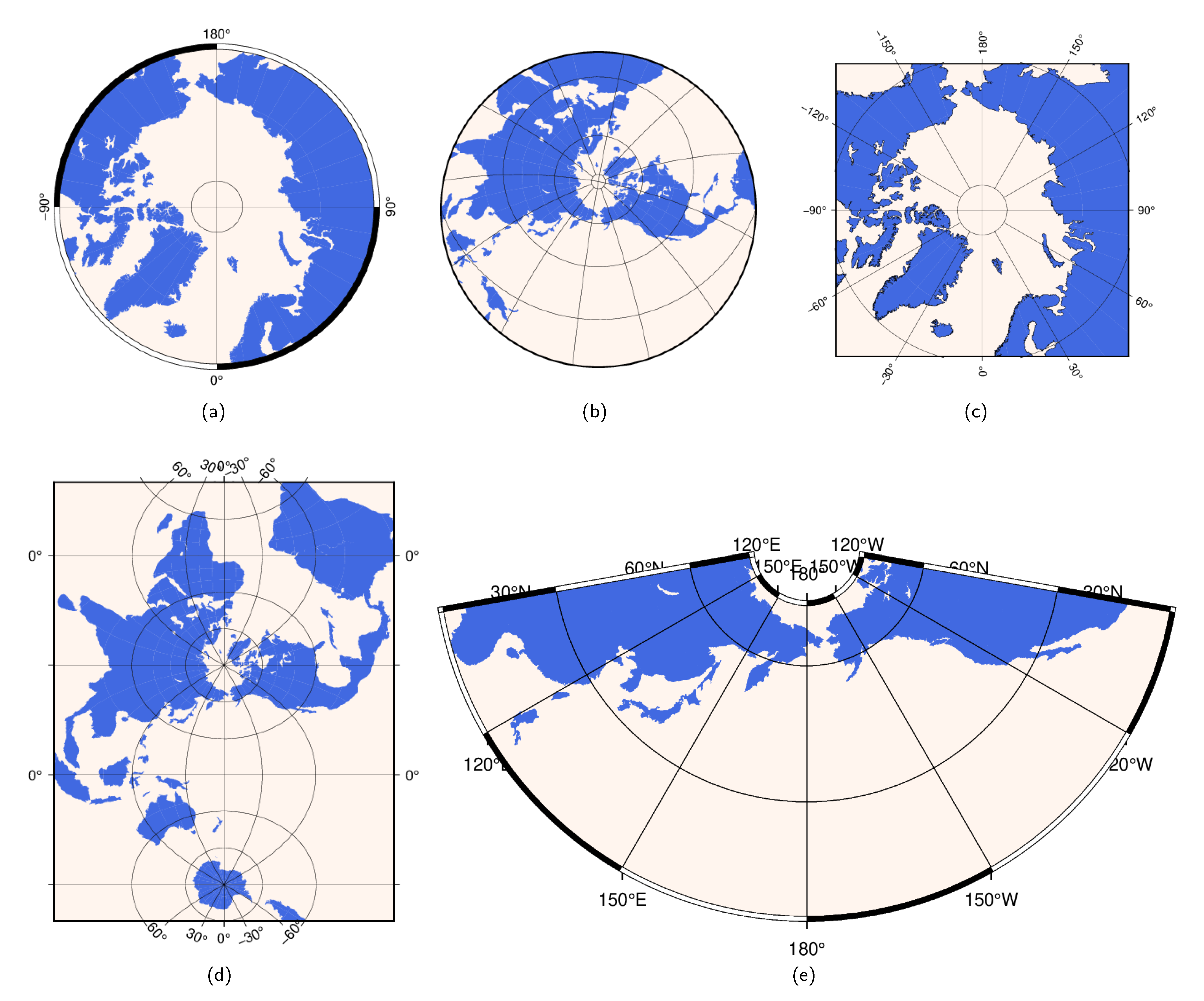
5.3.2. Polar Map Projections
- Novel polar projection methods. Researchers can continue to explore and develop new polar projection methods to address the existing issues in current projection methods. This may involve introducing more complex mathematical models or adopting new technologies such as machine learning and artificial intelligence to achieve more accurate and geographically realistic polar projections.
- Multiscale and multi-resolution polar projections. Polar regions encompass a wide range of scales, from local glaciers to the entire polar region, requiring map projections at different scales. Therefore, researchers can focus on how to perform effective polar projections at various scales and resolutions to meet diverse application requirements and data accuracy needs.
- Dynamic polar projections. The geographical environment in polar regions undergoes frequent changes, such as the melting of sea ice and glacier movements. Researchers can investigate how to address this dynamism by developing dynamic polar projection methods that can adapt to changes in the geographical environment, as well as techniques for real-time updating and presentation of geographic information.
- Multidimensional polar projections. In addition to spatial dimensions, data in polar regions also involve multiple dimensions such as time, temperature, and thickness. Researchers can explore how to effectively process and present multidimensional data within polar projections, enhancing the understanding of polar region changes and features.
6. Conclusions
Author Contributions
Funding
Data Availability Statement
Acknowledgments
Conflicts of Interest
References
- Zhou, L.; Zheng, S.; Ding, S.; Xie, C.; Liu, R. Influence of propeller on brash ice loads and pressure fluctuation for a reversing polar ship. Ocean Eng. 2023, 280, 114624. [Google Scholar] [CrossRef]
- Wessel, B.; Huber, M.; Wohlfart, C.; Bertram, A.; Osterkamp, N.; Marschalk, U.; Gruber, A.; Reuß, F.; Abdullahi, S.; Georg, I.; et al. TanDEM-X PolarDEM 90 m of Antarctica: Generation and error characterization. Cryosphere 2021, 15, 5241–5260. [Google Scholar] [CrossRef]
- Kurczyński, Z.; Różycki, S.; Bylina, P. Mapping of polar areas based on high-resolution satellite images: The example of the Henryk Arctowski Polish Antarctic Station. Rep. Geod. Geoinform. 2017, 104, 65–78. [Google Scholar] [CrossRef]
- Liu, J.; Yao, R.; Yu, L.; Gan, X.; Wang, X. Line design and optimization for polar expedition cruise ships with transoceanic voyage characteristics. J. Mar. Sci. Technol. 2023, 28, 270–287. [Google Scholar] [CrossRef]
- Chen, C. Science Mapping: A Systematic Review of the Literature. J. Data Inf. Sci. 2017, 2, 1–40. [Google Scholar] [CrossRef]
- Shokr, M.; Sinha, N.K. Sea Ice: Physics and Remote Sensing; John Wiley & Sons: Hoboken, NJ, USA, 2023. [Google Scholar]
- Murfitt, J.; Duguay, C.R. 50 years of lake ice research from active microwave remote sensing: Progress and prospects. Remote Sens. Environ. 2021, 264, 112616. [Google Scholar] [CrossRef]
- Lyu, H.; Huang, W.; Mahdianpari, M. A meta-analysis of sea ice monitoring using spaceborne polarimetric SAR: Advances in the last decade. IEEE J. Sel. Top. Appl. Earth Obs. Remote Sens. 2022, 15, 6158–6179. [Google Scholar] [CrossRef]
- Kang, J.; Tong, F.; Ding, X.; Li, S.; Zhu, R.; Huang, Y.; Xu, Y.; Fernandez-Beltran, R. Decoding the partial pretrained networks for sea-ice segmentation of 2021 gaofen challenge. IEEE J. Sel. Top. Appl. Earth Obs. Remote Sens. 2022, 15, 4521–4530. [Google Scholar] [CrossRef]
- Li, W.; Liu, L.; Zhang, J. Fusion of SAR and optical image for sea ice Extraction. J. Ocean Univ. China 2021, 20, 1440–1450. [Google Scholar] [CrossRef]
- Han, Y.; Liu, Y.; Hong, Z.; Zhang, Y.; Yang, S.; Wang, J. Sea ice image classification based on heterogeneous data fusion and deep learning. Remote Sens. 2021, 13, 592. [Google Scholar] [CrossRef]
- Han, Y.; Shi, X.; Wang, J.; Zhang, Y.; Hong, Z.; Ma, Z.; Zhou, R. Sea ice image classification based on ResFPG network and heterogeneous data fusion. Int. J. Remote Sens. 2022, 43, 6881–6898. [Google Scholar] [CrossRef]
- Zhang, X.; Zhou, Y.; Jin, J.; Wang, Y.; Fan, M.; Wang, N.; Zhang, Y. ICENETv2: A Fine-Grained River Ice Semantic Segmentation Network Based on UAV Images. Remote Sens. 2021, 13, 633. [Google Scholar] [CrossRef]
- Panchi, N.; Kim, E.; Bhattacharyya, A. Supplementing remote sensing of ice: Deep learning-based image segmentation system for automatic detection and localization of sea-ice formations from close-range optical images. IEEE Sens. J. 2021, 21, 18004–18019. [Google Scholar] [CrossRef]
- Wang, C.; Mouche, A.; Tandeo, P.; Stopa, J.E.; Longépé, N.; Erhard, G.; Foster, R.C.; Vandemark, D.; Chapron, B. A labelled ocean SAR imagery dataset of ten geophysical phenomena from Sentinel-1 wave mode. Geosci. Data J. 2019, 6, 105–115. [Google Scholar] [CrossRef]
- Zhang, X.; Jin, J.; Lan, Z.; Li, C.; Fan, M.; Wang, Y.; Yu, X.; Zhang, Y. ICENET: A semantic segmentation deep network for river ice by fusing positional and channel-wise attentive features. Remote Sens. 2020, 12, 221. [Google Scholar] [CrossRef]
- Zakhvatkina, N.; Smirnov, V.; Bychkova, I. Satellite SAR data-based sea ice classification: An overview. Geosciences 2019, 9, 152. [Google Scholar] [CrossRef]
- Dabboor, M.; Shokr, M. A new likelihood ratio for supervised classification of fully polarimetric SAR data: An application for sea-ice-type mapping. ISPRS J. Photogramm. Remote Sens. 2013, 84, 1–11. [Google Scholar] [CrossRef]
- Ashouri, Z.; Scott, A. A heuristic method to use ice andwater probabilities from SAR imagery to improve ice concentration estimates. In Proceedings of the 2014 IEEE Geoscience and Remote Sensing Symposium, Quebec City, QC, Canada, 13–18 July 2014; pp. 4868–4871. [Google Scholar]
- Wang, L.; Scott, K.A.; Clausi, D.A. Improved sea ice concentration estimation through fusing classified SAR imagery and AMSR-E data. Can. J. Remote Sens. 2016, 42, 41–52. [Google Scholar] [CrossRef]
- Clausi, D.; Qin, A.; Chowdhury, M.; Yu, P.; Maillard, P. MAGIC: MAp-guided ice classification system. Can. J. Remote Sens. 2010, 36, S13–S25. [Google Scholar] [CrossRef]
- Lohse, J.; Doulgeris, A.P.; Dierking, W. Mapping sea-ice types from Sentinel-1 considering the surface-type dependent effect of incidence angle. Ann. Glaciol. 2020, 61, 260–270. [Google Scholar] [CrossRef]
- Guo, W.; Itkin, P.; Singha, S.; Doulgeris, A.P.; Johansson, M.; Spreen, G. Sea ice classification of TerraSAR-X ScanSAR images for the MOSAiC expedition incorporating per-class incidence angle dependency of image texture. Cryosphere 2023, 17, 1279–1297. [Google Scholar] [CrossRef]
- Scott, K.A.; Ashouri, Z.; Buehner, M.; Pogson, L.; Carrieres, T. Assimilation of ice and water observations from SAR imagery to improve estimates of sea ice concentration. Tellus A Dyn. Meteorol. Oceanogr. 2015, 67, 27218. [Google Scholar] [CrossRef]
- Moen, M.A.; Anfinsen, S.N.; Doulgeris, A.P.; Renner, A.; Gerland, S. Assessing polarimetric SAR sea-ice classifications using consecutive day images. Ann. Glaciol. 2015, 56, 285–294. [Google Scholar] [CrossRef]
- Hillebrand, F.L.; de Carvalho Barreto, I.D.; Bremer, U.F.; Arigony-Neto, J.; Júnior, C.W.M.; Simões, J.C.; da Rosa, C.N.; de Jesus, J.B. Application of textural analysis to map the sea ice concentration with sentinel 1A in the western region of the Antarctic Peninsula. Polar Sci. 2021, 29, 100719. [Google Scholar] [CrossRef]
- Zhu, Y.; Yu, K.; Zou, J.; Wickert, J. Sea ice detection using GNSS-R delay-Doppler maps from UK TechDemoSat-1. In Proceedings of the 2017 IEEE International Geoscience and Remote Sensing Symposium (IGARSS), Fort Worth, TX, USA, 23–28 July 2017; pp. 4110–4113. [Google Scholar]
- Komarov, A.S.; Buehner, M. Adaptive probability thresholding in automated ice and open water detection from RADARSAT-2 images. IEEE Geosci. Remote Sens. Lett. 2018, 15, 552–556. [Google Scholar] [CrossRef]
- Zhang, X.; Ren, S. Automatic classification of SAR image based on r-gmm algorithm. In Proceedings of the 2018 11th International Congress on Image and Signal Processing, BioMedical Engineering and Informatics (CISP-BMEI), Beijing, China, 13–15 October 2018; pp. 1–5. [Google Scholar]
- Liu, J.; Scott, K.A.; Fieguth, P.W. Detection of marginal ice zone in Synthetic Aperture Radar imagery using curvelet-based features: A case study on the Canadian East Coast. J. Appl. Remote Sens. 2019, 13, 14505. [Google Scholar] [CrossRef]
- Xie, T.; Perrie, W.; Wei, C.; Zhao, L. Discrimination of open water from sea ice in the Labrador Sea using quad-polarized synthetic aperture radar. Remote Sens. Environ. 2020, 247, 111948. [Google Scholar] [CrossRef]
- Keller, M.R.; Gifford, C.M.; Winstead, N.S.; Walton, W.C.; Dietz, J.E. Active/passive multiple polarization sea ice detection during initial freeze-up. IEEE Trans. Geosci. Remote Sens. 2020, 59, 5434–5448. [Google Scholar] [CrossRef]
- Yu, Q.; Clausi, D.A. IRGS: Image segmentation using edge penalties and region growing. IEEE Trans. Pattern Anal. Mach. Intell. 2008, 30, 2126–2139. [Google Scholar]
- Leigh, S.; Wang, Z.; Clausi, D.A. Automated ice–water classification using dual polarization SAR satellite imagery. IEEE Trans. Geosci. Remote Sens. 2013, 52, 5529–5539. [Google Scholar] [CrossRef]
- Ghanbari, M.; Clausi, D.A.; Xu, L.; Jiang, M. Contextual classification of sea-ice types using compact polarimetric SAR data. IEEE Trans. Geosci. Remote Sens. 2019, 57, 7476–7491. [Google Scholar] [CrossRef]
- Ghanbari, M.; Clausi, D.A.; Xu, L.; Jiang, M. Unsupervised Segmentation of Multilook Compact Polarimetric Sar Data based on Complex Wishart Distribution. In Proceedings of the IGARSS 2020—2020 IEEE International Geoscience and Remote Sensing Symposium, Online, 26 September–2 October 2020; pp. 1456–1459. [Google Scholar] [CrossRef]
- Ghanbari, M.; Clausi, D.A.; Xu, L. CP-IRGS: A Region-Based Segmentation of Multilook Complex Compact Polarimetric SAR Data. IEEE J. Sel. Top. Appl. Earth Obs. Remote Sens. 2021, 14, 6559–6571. [Google Scholar] [CrossRef]
- Li, F.; Clausi, D.A.; Wang, L.; Xu, L. A semi-supervised approach for ice–water classification using dual-polarization SAR satellite imagery. In Proceedings of the IEEE Conference on Computer Vision and Pattern Recognition Workshops, Boston, MA, USA, 7–12 June 2015; pp. 28–35. [Google Scholar]
- Wang, J.; Duguay, C.R.; Clausi, D.A.; Pinard, V.; Howell, S.E. Semi-automated classification of lake ice cover using dual polarization RADARSAT-2 imagery. Remote Sens. 2018, 10, 1727. [Google Scholar] [CrossRef]
- Hoekstra, M.; Jiang, M.; Clausi, D.A.; Duguay, C. Lake ice–water classification of RADARSAT-2 images by integrating IRGS segmentation with pixel-based random forest labeling. Remote Sens. 2020, 12, 1425. [Google Scholar] [CrossRef]
- Jiang, M.; Xu, L.; Clausi, D.A. Sea ice–water classification of RADARSAT-2 imagery based on residual neural networks (ResNet) with regional pooling. Remote Sens. 2022, 14, 3025. [Google Scholar] [CrossRef]
- Jiang, M.; Clausi, D.A.; Xu, L. Sea-Ice Mapping of RADARSAT-2 Imagery by Integrating Spatial Contexture With Textural Features. IEEE J. Sel. Top. Appl. Earth Obs. Remote Sens. 2022, 15, 7964–7977. [Google Scholar] [CrossRef]
- Jiang, M.; Chen, X.; Xu, L.; Clausi, D.A. Semi-supervised sea ice classification of SAR imagery based on graph convolutional network. In Proceedings of the IGARSS 2022—2022 IEEE International Geoscience and Remote Sensing Symposium, Kuala Lumpur, Malaysia, 17–22 July 2022; pp. 1031–1034. [Google Scholar]
- Chen, X.; Scott, K.A.; Xu, L.; Jiang, M.; Fang, Y.; Clausi, D.A. Uncertainty-Incorporated Ice and Open Water Detection on Dual-polarized SAR Sea Ice Imagery. IEEE Trans. Geosci. Remote Sens. 2023, 61, 1–13. [Google Scholar] [CrossRef]
- Han, H.; Hong, S.H.; Kim, H.c.; Chae, T.B.; Choi, H.J. A study of the feasibility of using KOMPSAT-5 SAR data to map sea ice in the Chukchi Sea in late summer. Remote Sens. Lett. 2017, 8, 468–477. [Google Scholar] [CrossRef]
- Dabboor, M.; Montpetit, B.; Howell, S. Assessment of simulated compact polarimetry of the high resolution radarsat constellation mission SAR mode for multiyear and first year sea ice characterization. In Proceedings of the IGARSS 2018—2018 IEEE International Geoscience and Remote Sensing Symposium, Valencia, Spain, 22–27 July 2018; pp. 2420–2423. [Google Scholar]
- Gegiuc, A.; Similä, M.; Karvonen, J.; Lensu, M.; Mäkynen, M.; Vainio, J. Estimation of degree of sea ice ridging based on dual-polarized C-band SAR data. Cryosphere 2018, 12, 343–364. [Google Scholar] [CrossRef]
- Han, H.; Kim, H.C. Evaluation of summer passive microwave sea ice concentrations in the Chukchi Sea based on KOMPSAT-5 SAR and numerical weather prediction data. Remote Sens. Environ. 2018, 209, 343–362. [Google Scholar] [CrossRef]
- Tan, W.; Li, J.; Xu, L.; Chapman, M.A. Semiautomated segmentation of Sentinel-1 SAR imagery for mapping sea ice in Labrador coast. IEEE J. Sel. Top. Appl. Earth Obs. Remote Sens. 2018, 11, 1419–1432. [Google Scholar] [CrossRef]
- Murashkin, D.; Spreen, G.; Huntemann, M.; Dierking, W. Method for detection of leads from Sentinel-1 SAR images. Ann. Glaciol. 2018, 59, 124–136. [Google Scholar] [CrossRef]
- Marcaccio, J.V.; Gardner Costa, J.; Brooks, J.L.; Boston, C.M.; Cooke, S.J.; Midwood, J.D. Automated Coastal Ice Mapping with SAR Can Inform Winter Fish Ecology in the Laurentian Great Lakes. Can. J. Remote Sens. 2022, 48, 19–36. [Google Scholar] [CrossRef]
- Yang, X.; Pavelsky, T.M.; Bendezu, L.P.; Zhang, S. Simple method to extract lake ice condition from landsat images. IEEE Trans. Geosci. Remote Sens. 2021, 60, 1–10. [Google Scholar] [CrossRef]
- Park, J.W.; Korosov, A.A.; Babiker, M.; Won, J.S.; Hansen, M.W.; Kim, H.C. Classification of sea-ice-types in Sentinel-1 synthetic aperture radar images. Cryosphere 2020, 14, 2629–2645. [Google Scholar] [CrossRef]
- Park, J.W.; Korosov, A.; Babiker, M.; Kim, H.C. Automated sea ice classification using Sentinel-1 imagery. In Proceedings of the IGARSS 2019—2019 IEEE International Geoscience and Remote Sensing Symposium, Yokohama, Japan, 28 July–2 August 2019; pp. 4008–4011. [Google Scholar]
- Ressel, R.; Singha, S.; Lehner, S. Evaluating suitability of Pol-SAR (TerraSAR-X, Radarsat-2) for automated sea ice classification. In Proceedings of the Land Surface and Cryosphere Remote Sensing III, SPIE, New Delhi, India, 4–7 April 2016; Volume 9877, pp. 137–150. [Google Scholar]
- Ressel, R.; Singha, S.; Lehner, S.; Rösel, A.; Spreen, G. Investigation into different polarimetric features for sea ice classification using X-band synthetic aperture radar. IEEE J. Sel. Top. Appl. Earth Obs. Remote Sens. 2016, 9, 3131–3143. [Google Scholar] [CrossRef]
- Aldenhoff, W.; Heuzé, C.; Eriksson, L.E. Comparison of ice/water classification in Fram Strait from C-and L-band SAR imagery. Ann. Glaciol. 2018, 59, 112–123. [Google Scholar] [CrossRef]
- Singha, S.; Johansson, M.; Hughes, N.; Hvidegaard, S.M.; Skourup, H. Arctic Sea Ice Characterization Using Spaceborne Fully Polarimetric L-, C-, and X-Band SAR With Validation by Airborne Measurements. IEEE Trans. Geosci. Remote Sens. 2018, 56, 3715–3734. [Google Scholar] [CrossRef]
- Singha, S.; Johansson, A.M.; Doulgeris, A.P. Robustness of SAR sea-ice-type classification across incidence angles and seasons at L-band. IEEE Trans. Geosci. Remote Sens. 2020, 59, 9941–9952. [Google Scholar] [CrossRef]
- Karvonen, J. A sea ice concentration estimation algorithm utilizing radiometer and SAR data. Cryosphere 2014, 8, 1639–1650. [Google Scholar] [CrossRef]
- Karvonen, J. Baltic sea ice concentration estimation using SENTINEL-1 SAR and AMSR2 microwave radiometer data. IEEE Trans. Geosci. Remote Sens. 2017, 55, 2871–2883. [Google Scholar] [CrossRef]
- Yan, Q.; Huang, W.; Moloney, C. Neural networks based sea ice detection and concentration retrieval from GNSS-R delay-Doppler maps. IEEE J. Sel. Top. Appl. Earth Obs. Remote Sens. 2017, 10, 3789–3798. [Google Scholar] [CrossRef]
- Asadi, N.; Scott, K.A.; Komarov, A.S.; Buehner, M.; Clausi, D.A. Evaluation of a neural network with uncertainty for detection of ice and water in SAR imagery. IEEE Trans. Geosci. Remote Sens. 2020, 59, 247–259. [Google Scholar] [CrossRef]
- Liu, H.; Guo, H.; Zhang, L. SVM-based sea ice classification using textural features and concentration from RADARSAT-2 dual-pol ScanSAR data. IEEE J. Sel. Top. Appl. Earth Obs. Remote Sens. 2014, 8, 1601–1613. [Google Scholar] [CrossRef]
- Zakhvatkina, N.; Korosov, A.; Muckenhuber, S.; Sandven, S.; Babiker, M. Operational algorithm for ice–water classification on dual-polarized RADARSAT-2 images. Cryosphere 2017, 11, 33–46. [Google Scholar] [CrossRef]
- Liu, H.; Guo, H.; Li, X.M.; Zhang, L. An approach to discrimination of sea ice from open water using SAR data. In Proceedings of the 2016 IEEE International Geoscience and Remote Sensing Symposium (IGARSS), Beijing, China, 10–15 July 2016; pp. 4865–4867. [Google Scholar]
- Hong, D.B.; Yang, C.S. Automatic discrimination approach of sea ice in the Arctic Ocean using Sentinel-1 Extra Wide Swath dual-polarized SAR data. Int. J. Remote Sens. 2018, 39, 4469–4483. [Google Scholar] [CrossRef]
- Li, X.M.; Sun, Y.; Zhang, Q. Extraction of sea ice cover by Sentinel-1 SAR based on support vector machine with unsupervised generation of training data. IEEE Trans. Geosci. Remote Sens. 2020, 59, 3040–3053. [Google Scholar] [CrossRef]
- Zhang, L.; Liu, H.; Gu, X.; Guo, H.; Chen, J.; Liu, G. Sea ice classification using TerraSAR-X ScanSAR data with removal of scalloping and interscan banding. IEEE J. Sel. Top. Appl. Earth Obs. Remote Sens. 2019, 12, 589–598. [Google Scholar] [CrossRef]
- Yan, Q.; Huang, W. Detecting sea ice from TechDemoSat-1 data using support vector machines with feature selection. IEEE J. Sel. Top. Appl. Earth Obs. Remote Sens. 2019, 12, 1409–1416. [Google Scholar] [CrossRef]
- Yan, Q.; Huang, W. Sea ice concentration estimation from TechDemoSat-1 data using support vector regression. In Proceedings of the 2019 IEEE Radar Conference (RadarConf), Boston, MA, USA, 22–26 April 2019; pp. 1–6. [Google Scholar]
- Zhu, T.; Li, F.; Heygster, G.; Zhang, S. Antarctic sea-ice classification based on conditional random fields from RADARSAT-2 dual-polarization satellite images. IEEE J. Sel. Top. Appl. Earth Obs. Remote Sens. 2016, 9, 2451–2467. [Google Scholar] [CrossRef]
- Han, Y.; Zhao, Y.; Zhang, Y.; Wang, J.; Yang, S.; Hong, Z.; Cao, S. A cooperative framework based on active and semi-supervised learning for sea ice classification using eo-1 hyperion data. Trans. Jpn. Soc. Aeronaut. Space Sci. 2019, 62, 318–330. [Google Scholar] [CrossRef]
- Barbieux, K.; Charitsi, A.; Merminod, B. Icy lakes extraction and water-ice classification using Landsat 8 OLI multispectral data. Int. J. Remote Sens. 2018, 39, 3646–3678. [Google Scholar] [CrossRef]
- Lohse, J.; Doulgeris, A.P.; Dierking, W. An optimal decision-tree design strategy and its application to sea ice classification from SAR imagery. Remote Sens. 2019, 11, 1574. [Google Scholar] [CrossRef]
- Komarov, A.S.; Buehner, M. Automated detection of ice and open water from dual-polarization RADARSAT-2 images for data assimilation. IEEE Trans. Geosci. Remote Sens. 2017, 55, 5755–5769. [Google Scholar] [CrossRef]
- Komarov, A.S.; Buehner, M. Ice concentration from dual-polarization SAR images using ice and water retrievals at multiple spatial scales. IEEE Trans. Geosci. Remote Sens. 2020, 59, 950–961. [Google Scholar] [CrossRef]
- Chen, S.; Yan, Y.; Ren, J.; Hwang, B.; Marshall, S.; Durrani, T. Superpixel Based Sea Ice Segmentation with High-Resolution Optical Images: Analysis and Evaluation. In Proceedings of the Communications, Signal Processing, and Systems: Proceedings of the 10th International Conference on Communications, Signal Processing, and Systems, Changbaishan, China, 24–25 July 2021; Springer: Singapore, 2022; Volume 2, pp. 474–482. [Google Scholar]
- Wang, B.; Xia, L.; Song, D.; Li, Z.; Wang, N. A two-round weight voting strategy-based ensemble learning method for sea ice classification of sentinel-1 imagery. Remote Sens. 2021, 13, 3945. [Google Scholar] [CrossRef]
- Kim, M.; Kim, H.C.; Im, J.; Lee, S.; Han, H. Object-based landfast sea ice detection over West Antarctica using time series ALOS PALSAR data. Remote Sens. Environ. 2020, 242, 111782. [Google Scholar] [CrossRef]
- Liu, M.; Yan, R.; Zhang, J.; Xu, Y.; Chen, P.; Shi, L.; Wang, J.; Zhong, S.; Zhang, X. Arctic sea ice classification based on CFOSAT SWIM data at multiple small incidence angles. Remote Sens. 2022, 14, 91. [Google Scholar] [CrossRef]
- Ren, S.; Zhang, X. A New GMRF Self-supervised Algorithm Applied to SAR Image Classification. J. Indian Soc. Remote Sens. 2021, 49, 1569–1580. [Google Scholar] [CrossRef]
- Song, W.; Gao, W.; He, Q.; Liotta, A.; Guo, W. Si-stsar-7: A large sar images dataset with spatial and temporal information for classification of winter sea ice in hudson bay. Remote Sens. 2022, 14, 168. [Google Scholar] [CrossRef]
- Wang, L.; Scott, K.A.; Xu, L.; Clausi, D.A. Sea ice concentration estimation during melt from dual-pol SAR scenes using deep convolutional neural networks: A case study. IEEE Trans. Geosci. Remote Sens. 2016, 54, 4524–4533. [Google Scholar] [CrossRef]
- Wang, L.; Scott, K.A.; Clausi, D.A.; Xu, Y. Ice concentration estimation in the gulf of St. Lawrence using fully convolutional neural network. In Proceedings of the 2017 IEEE International Geoscience and Remote Sensing Symposium (IGARSS), Fort Worth, TX, USA, 23–28 July 2017; pp. 4991–4994. [Google Scholar]
- Wang, L.; Scott, K.A.; Clausi, D.A. Sea ice concentration estimation during freeze-up from SAR imagery using a convolutional neural network. Remote Sens. 2017, 9, 408. [Google Scholar] [CrossRef]
- Li, J.; Wang, C.; Wang, S.; Zhang, H.; Fu, Q.; Wang, Y. Gaofen-3 sea ice detection based on deep learning. In Proceedings of the 2017 Progress in Electromagnetics Research Symposium-Fall (PIERS-FALL), Singapore, 19–22 November 2017; pp. 933–939. [Google Scholar]
- Yan, Q.; Huang, W. Sea ice sensing from GNSS-R data using convolutional neural networks. IEEE Geosci. Remote Sens. Lett. 2018, 15, 1510–1514. [Google Scholar] [CrossRef]
- Yan, Q.; Huang, W. Convolutional Neural Networks-Based Sea Ice Detection From TDS-1 Data. In Proceedings of the 2018 18th International Symposium on Antenna Technology and Applied Electromagnetics (ANTEM), Waterloo, ON, Canada, 19–22 August 2018; pp. 1–2. [Google Scholar]
- Han, Y.; Gao, Y.; Zhang, Y.; Wang, J.; Yang, S. Hyperspectral sea ice image classification based on the spectral-spatial-joint feature with deep learning. Remote Sens. 2019, 11, 2170. [Google Scholar] [CrossRef]
- Boulze, H.; Korosov, A.; Brajard, J. Classification of sea-ice-types in Sentinel-1 SAR data using convolutional neural networks. Remote Sens. 2020, 12, 2165. [Google Scholar] [CrossRef]
- Karvonen, J. Baltic sea ice concentration estimation from c-band dual-polarized sar imagery by image segmentation and convolutional neural networks. IEEE Trans. Geosci. Remote Sens. 2021, 60, 1–11. [Google Scholar] [CrossRef]
- Malmgren-Hansen, D.; Pedersen, L.T.; Nielsen, A.A.; Kreiner, M.B.; Saldo, R.; Skriver, H.; Lavelle, J.; Buus-Hinkler, J.; Krane, K.H. A convolutional neural network architecture for Sentinel-1 and AMSR2 data fusion. IEEE Trans. Geosci. Remote Sens. 2020, 59, 1890–1902. [Google Scholar] [CrossRef]
- Han, Y.; Wei, C.; Zhou, R.; Hong, Z.; Zhang, Y.; Yang, S. Combining 3D-CNN and squeeze-and-excitation networks for remote sensing sea ice image classification. Math. Probl. Eng. 2020, 2020, 1–15. [Google Scholar] [CrossRef]
- Han, Y.; Shi, X.; Yang, S.; Zhang, Y.; Hong, Z.; Zhou, R. Hyperspectral Sea Ice Image Classification Based on the Spectral-Spatial-Joint Feature with the PCA Network. Remote Sens. 2021, 13, 2253. [Google Scholar] [CrossRef]
- Xu, Y.; Scott, K.A. Sea ice and open water classification of SAR imagery using CNN-based transfer learning. In Proceedings of the 2017 IEEE International Geoscience and Remote Sensing Symposium (IGARSS), Fort Worth, TX, USA, 23–28 July 2017; pp. 3262–3265. [Google Scholar]
- Xu, Y.; Scott, K.A. Impact of intermediate ice concentration training data on sea ice concentration estimates from a convolutional neural network. Int. J. Remote Sens. 2019, 40, 5799–5811. [Google Scholar] [CrossRef]
- Khaleghian, S.; Ullah, H.; Kræmer, T.; Hughes, N.; Eltoft, T.; Marinoni, A. Sea ice classification of SAR imagery based on convolution neural networks. Remote Sens. 2021, 13, 1734. [Google Scholar] [CrossRef]
- Huang, G.; Liu, Z.; Van Der Maaten, L.; Weinberger, K.Q. Densely connected convolutional networks. In Proceedings of the IEEE Conference on Computer Vision and Pattern Recognition, Honolulu, HI, USA, 21–26 July 2017; pp. 4700–4708. [Google Scholar]
- Cooke, C.L.; Scott, K.A. Estimating sea ice concentration from SAR: Training convolutional neural networks with passive microwave data. IEEE Trans. Geosci. Remote Sens. 2019, 57, 4735–4747. [Google Scholar] [CrossRef]
- Nagi, A.S.; Minhas, M.S.; Xu, L.; Scott, K.A. A Multi-Scale Technique to Detect Marginal Ice Zones Using Convolutional Neural Networks. In Proceedings of the IGARSS 2020—2020 IEEE International Geoscience and Remote Sensing Symposium, Online, 26 September–2 October 2020; pp. 3035–3038. [Google Scholar]
- Kruk, R.; Fuller, M.C.; Komarov, A.S.; Isleifson, D.; Jeffrey, I. Proof of concept for sea ice stage of development classification using deep learning. Remote Sens. 2020, 12, 2486. [Google Scholar] [CrossRef]
- Lyu, H.; Huang, W.; Mahdianpari, M. Eastern arctic sea ice sensing: First results from the RADARSAT Constellation Mission data. Remote Sens. 2022, 14, 1165. [Google Scholar] [CrossRef]
- Brock, A.; De, S.; Smith, S.L.; Simonyan, K. High-performance large-scale image recognition without normalization. In Proceedings of the International Conference on Machine Learning, PMLR, Online, 18–24 July 2021; pp. 1059–1071. [Google Scholar]
- Song, W.; Li, M.; He, Q.; Huang, D.; Perra, C.; Liotta, A. A residual convolution neural network for sea ice classification with Sentinel-1 SAR imagery. In Proceedings of the 2018 IEEE International Conference on Data Mining Workshops (ICDMW), Singapore, 17–20 November 2018; pp. 795–802. [Google Scholar]
- Song, W.; Li, M.; Gao, W.; Huang, D.; Ma, Z.; Liotta, A.; Perra, C. Automatic sea-ice classification of SAR images based on spatial and temporal features learning. IEEE Trans. Geosci. Remote Sens. 2021, 59, 9887–9901. [Google Scholar] [CrossRef]
- Kortum, K.; Singha, S.; Spreen, G. Robust Multiseasonal Ice Classification From High-Resolution X-Band SAR. IEEE Trans. Geosci. Remote Sens. 2022, 60, 1–12. [Google Scholar] [CrossRef]
- Zhang, J.; Zhang, W.; Hu, Y.; Chu, Q.; Liu, L. An improved sea ice classification algorithm with Gaofen-3 dual-polarization SAR data based on deep convolutional neural networks. Remote Sens. 2022, 14, 906. [Google Scholar] [CrossRef]
- Tamber, M.S.; Scott, K.A.; Pedersen, L.T. Accounting for label errors when training a convolutional neural network to estimate sea ice concentration using operational ice charts. IEEE J. Sel. Top. Appl. Earth Obs. Remote Sens. 2022, 15, 1502–1513. [Google Scholar] [CrossRef]
- Ren, Y.; Xu, H.; Liu, B.; Li, X. Sea ice and open water classification of SAR images using a deep learning model. In Proceedings of the IGARSS 2020—2020 IEEE International Geoscience and Remote Sensing Symposium, Online, 26 September–2 October 2020; pp. 3051–3054. [Google Scholar]
- Ren, Y.; Li, X.; Yang, X.; Xu, H. Development of a dual-attention U-Net model for sea ice and open water classification on SAR images. IEEE Geosci. Remote Sens. Lett. 2021, 19, 1–5. [Google Scholar] [CrossRef]
- Ren, Y.; Li, X.; Yang, X.; Xu, H. Sea Ice Detection from SAR Images Based on Deep Fully Convolutional Networks. In Artificial Intelligence Oceanography; Springer: Singapore, 2023; pp. 253–276. [Google Scholar]
- Ji, W.; Fang, Z.; Feng, D.; Ge, X. Semantic segmentation of Arctic Sea ice in summer from remote sensing satellite images based on BAU-NET. J. Appl. Remote Sens. 2022, 16, 046514. [Google Scholar] [CrossRef]
- De Gelis, I.; Colin, A.; Longépé, N. Prediction of categorized sea ice concentration from Sentinel-1 SAR images based on a fully convolutional network. IEEE J. Sel. Top. Appl. Earth Obs. Remote Sens. 2021, 14, 5831–5841. [Google Scholar] [CrossRef]
- Radhakrishnan, K.; Scott, K.A.; Clausi, D.A. Sea ice concentration estimation: Using passive microwave and SAR data with a U-net and curriculum learning. IEEE J. Sel. Top. Appl. Earth Obs. Remote Sens. 2021, 14, 5339–5351. [Google Scholar] [CrossRef]
- Wang, Y.R.; Li, X.M. Arctic sea ice cover data from spaceborne synthetic aperture radar by deep learning. Earth Syst. Sci. Data 2021, 13, 2723–2742. [Google Scholar] [CrossRef]
- Stokholm, A.; Wulf, T.; Kucik, A.; Saldo, R.; Buus-Hinkler, J.; Hvidegaard, S.M. AI4SeaIce: Toward solving ambiguous SAR textures in convolutional neural networks for automatic sea ice concentration charting. IEEE Trans. Geosci. Remote Sens. 2022, 60, 1–13. [Google Scholar] [CrossRef]
- Nagi, A.S.; Kumar, D.; Sola, D.; Scott, K.A. RUF: Effective sea ice floe segmentation using end-to-end RES-UNET-CRF with dual loss. Remote Sens. 2021, 13, 2460. [Google Scholar] [CrossRef]
- Song, W.; Li, H.; He, Q.; Gao, G.; Liotta, A. E-MPSPNet: Ice–Water SAR Scene Segmentation Based on Multi-Scale Semantic Features and Edge Supervision. Remote Sens. 2022, 14, 5753. [Google Scholar] [CrossRef]
- Zhou, Z.; Rahman Siddiquee, M.M.; Tajbakhsh, N.; Liang, J. Unet++: A nested u-net architecture for medical image segmentation. In Proceedings of the Deep Learning in Medical Image Analysis and Multimodal Learning for Clinical Decision Support: 4th International Workshop, DLMIA 2018, and 8th International Workshop, ML-CDS 2018, Held in Conjunction with MICCAI 2018, Granada, Spain, 20 September 2018; Proceedings 4. Springer: Cham, Switzerland, 2018; pp. 3–11. [Google Scholar]
- Murashkin, D.; Frost, A. Arctic Sea ICE Mapping Using Sentinel-1 SAR Scenes with a Convolutional Neural Network. In Proceedings of the 2021 IEEE International Geoscience and Remote Sensing Symposium IGARSS, Brussels, Belgium, 11–16 July 2021; pp. 5660–5663. [Google Scholar]
- Feng, T.; Liu, X.; Li, R. Super-Resolution-Aided Sea Ice Concentration Estimation from AMSR2 Images by Encoder-Decoder Networks with Atrous Convolution. IEEE J. Sel. Top. Appl. Earth Obs. Remote Sens. 2022, 16, 962–973. [Google Scholar] [CrossRef]
- Zhang, E.; Liu, L.; Huang, L.; Ng, K.S. An automated, generalized, deep-learning-based method for delineating the calving fronts of Greenland glaciers from multi-sensor remote sensing imagery. Remote Sens. Environ. 2021, 254, 112265. [Google Scholar] [CrossRef]
- Chen, X.; Scott, K.A.; Jiang, M.; Fang, Y.; Xu, L.; Clausi, D.A. Sea Ice Classification With Dual-Polarized SAR Imagery: A Hierarchical Pipeline. In Proceedings of the IEEE/CVF Winter Conference on Applications of Computer Vision, Waikoloa, HI, USA, 3–7 January 2023; pp. 224–232. [Google Scholar]
- Colin, A.; Fablet, R.; Tandeo, P.; Husson, R.; Peureux, C.; Longépé, N.; Mouche, A. Semantic segmentation of metoceanic processes using SAR observations and deep learning. Remote Sens. 2022, 14, 851. [Google Scholar] [CrossRef]
- Hoffman, J.P.; Ackerman, S.A.; Liu, Y.; Key, J.R.; McConnell, I.L. Application of a convolutional neural network for the detection of sea ice leads. Remote Sens. 2021, 13, 4571. [Google Scholar] [CrossRef]
- Aryal, B.; Miles, K.E.; Zesati, S.A.V.; Fuentes, O. Boundary Aware U-Net for Glacier Segmentation. arXiv 2023, arXiv:2301.11454. [Google Scholar] [CrossRef] [PubMed]
- Ma, Z.; Liu, Z.; Pu, J.; Xu, L.; Li, K.; Wangqu, L.; Wu, R.; Ma, Y.; Chen, Y.; Duguay, C. Deep convolutional neural network with random field model for lake ice mapping from Sentinel-1 imagery. Int. J. Remote Sens. 2021, 42, 9351–9375. [Google Scholar] [CrossRef]
- Wang, S.; Peppa, M.V.; Xiao, W.; Maharjan, S.B.; Joshi, S.P.; Mills, J.P. A second-order attention network for glacial lake segmentation from remotely sensed imagery. ISPRS J. Photogramm. Remote Sens. 2022, 189, 289–301. [Google Scholar] [CrossRef]
- Dowden, B.; De Silva, O.; Huang, W.; Oldford, D. Sea ice classification via deep neural network semantic segmentation. IEEE Sens. J. 2020, 21, 11879–11888. [Google Scholar] [CrossRef]
- Balasooriya, N.; Dowden, B.; Chen, J.; De Silva, O.; Huang, W. In-situ sea ice detection using DeepLabv3 semantic segmentation. In Proceedings of the OCEANS 2021: San Diego–Porto, San Diego, CA, USA, 20–23 September 2021; pp. 1–7. [Google Scholar]
- Alsharay, N.M.; Chen, Y.; Dobre, O.A.; De Silva, O. Improved Sea-Ice Identification Using Semantic Segmentation With Raindrop Removal. IEEE Access 2022, 10, 21599–21607. [Google Scholar] [CrossRef]
- Alsharay, N.M.; Dobre, O.A.; Chen, Y.; De Silva, O. Sea-Ice Classification Using Conditional Generative Adversarial Networks. IEEE Sens. Lett. 2023, 7, 1–4. [Google Scholar] [CrossRef]
- Zhang, C.; Chen, X.; Ji, S. Semantic image segmentation for sea ice parameters recognition using deep convolutional neural networks. Int. J. Appl. Earth Obs. Geoinf. 2022, 112, 102885. [Google Scholar] [CrossRef]
- Zhao, J.; Chen, L.; Li, J.; Zhao, Y. Semantic Segmentation of Sea Ice Based on U-net Network Modification. In Proceedings of the 2022 IEEE International Conference on Robotics and Biomimetics (ROBIO), Xishuangbanna, China, 5–9 December 2022; pp. 1151–1156. [Google Scholar]
- Chen, L.; Zhao, J.; Tian, K.; Zhao, Y. AM-ResNet: An Attention-Based Multi-Label Classification Network. In Proceedings of the 2022 IEEE International Conference on Robotics and Biomimetics (ROBIO), Xishuangbanna, China, 5–9 December 2022; pp. 380–384. [Google Scholar]
- Chen, L.; Zhao, J.; Li, W.; Zhao, Y. Navigation Environment Detection in Ice Area Based on Vibration of Ship Main Engine. In Proceedings of the 2022 IEEE International Conference on Robotics and Biomimetics (ROBIO), Xishuangbanna, China, 5–9 December 2022; pp. 1162–1166. [Google Scholar]
- Kim, Y.J.; Kim, H.C.; Han, D.; Lee, S.; Im, J. Prediction of monthly Arctic sea ice concentrations using satellite and reanalysis data based on convolutional neural networks. Cryosphere 2020, 14, 1083–1104. [Google Scholar] [CrossRef]
- Andersson, T.R.; Hosking, J.S.; Pérez-Ortiz, M.; Paige, B.; Elliott, A.; Russell, C.; Law, S.; Jones, D.C.; Wilkinson, J.; Phillips, T.; et al. Seasonal Arctic sea ice forecasting with probabilistic deep learning. Nat. Commun. 2021, 12, 5124. [Google Scholar] [CrossRef]
- Chen, X.; Valencia, R.; Soleymani, A.; Scott, K.A. Predicting Sea Ice Concentration With Uncertainty Quantification Using Passive Microwave and Reanalysis Data: A Case Study in Baffin Bay. IEEE Trans. Geosci. Remote Sens. 2023, 61, 1–13. [Google Scholar] [CrossRef]
- Gao, Y.; Gao, F.; Dong, J.; Wang, S. Sea ice change detection in SAR images based on collaborative representation. In Proceedings of the IGARSS 2018—2018 IEEE International Geoscience and Remote Sensing Symposium, Valencia, Spain, 22-27 July 2018; pp. 7320–7323. [Google Scholar]
- Gao, Y.; Gao, F.; Dong, J.; Wang, S. Transferred deep learning for sea ice change detection from synthetic-aperture radar images. IEEE Geosci. Remote Sens. Lett. 2019, 16, 1655–1659. [Google Scholar] [CrossRef]
- Qi, G.J.; Luo, J. Small data challenges in big data era: A survey of recent progress on unsupervised and semi-supervised methods. IEEE Trans. Pattern Anal. Mach. Intell. 2020, 44, 2168–2187. [Google Scholar] [CrossRef] [PubMed]
- Staccone, F. Deep Learning for Sea-Ice Classification on Synthetic Aperture Radar (SAR) Images in Earth Observation: Classification Using Semi-Supervised Generative Adversarial Networks on Partially Labeled Data. Master’s Thesis, Politecnico di Milano, Milan, Italy, 2020. [Google Scholar]
- Khaleghian, S.; Ullah, H.; Kræmer, T.; Eltoft, T.; Marinoni, A. Deep semisupervised teacher–student model based on label propagation for sea ice classification. IEEE J. Sel. Top. Appl. Earth Obs. Remote Sens. 2021, 14, 10761–10772. [Google Scholar] [CrossRef]
- Gonçalves, B.C.; Lynch, H.J. Fine-scale sea ice segmentation for high-resolution satellite imagery with weakly-supervised CNNs. Remote Sens. 2021, 13, 3562. [Google Scholar] [CrossRef]
- Huang, Z.; Dumitru, C.O.; Ren, J. Physics-aware feature learning of sar images with deep neural networks: A case study. In Proceedings of the 2021 IEEE International Geoscience and Remote Sensing Symposium IGARSS, Brussels, Belgium, 11–16 July 2021; pp. 1264–1267. [Google Scholar]
- Huang, Z.; Yao, X.; Liu, Y.; Dumitru, C.O.; Datcu, M.; Han, J. Physically explainable CNN for SAR image classification. ISPRS J. Photogramm. Remote Sens. 2022, 190, 25–37. [Google Scholar] [CrossRef]
- Liu, Y.; Huang, Z.; Han, J. Aleatoric Uncertainty Embedded Transfer Learning for SEA-ICE Classification in SAR Images. In Proceedings of the IGARSS 2022—2022 IEEE International Geoscience and Remote Sensing Symposium, Kuala Lumpur, Malaysia, 17–22 July 2022; pp. 4980–4983. [Google Scholar]
- Mahmud, M.S.; Nandan, V.; Singha, S.; Howell, S.E.; Geldsetzer, T.; Yackel, J.; Montpetit, B. C- and L-band SAR signatures of Arctic sea ice during freeze-up. Remote Sens. Environ. 2022, 279, 113129. [Google Scholar] [CrossRef]
- Temimi, M.; Abdelkader, M.; Tounsi, A.; Chaouch, N.; Carter, S.; Sjoberg, B.; Macneil, A.; Bingham-Maas, N. An Automated System to Monitor River Ice Conditions Using Visible Infrared Imaging Radiometer Suite Imagery. Remote Sens. 2023, 15, 4896. [Google Scholar] [CrossRef]
- Singh, A.; Kalke, H.; Loewen, M.; Ray, N. River ice segmentation with deep learning. IEEE Trans. Geosci. Remote Sens. 2020, 58, 7570–7579. [Google Scholar] [CrossRef]
- Rogers, T.; Walsh, J.; Rupp, T.; Brigham, L.; Sfraga, M. Future Arctic marine access: Analysis and evaluation of observations, models, and projections of sea ice. Cryosphere 2013, 7, 321–332. [Google Scholar] [CrossRef]
- Chang, K.Y.; He, S.; Chou, C.; Kao, S.L.; Chiou, A. Route planning and cost analysis for travelling through the Arctic Northeast Passage using public 3D GIS. Int. J. Geogr. Inf. Sci. 2015, 29, 1375–1393. [Google Scholar] [CrossRef]
- Chen, J.L.; Kang, S.C.; Meng, X.H.; You, Q.L. Assessments of the Arctic amplification and the changes in the Arctic sea surface. Adv. Clim. Change Res. 2019, 10, 193–202. [Google Scholar] [CrossRef]
- Mäkynen, M.; Haapala, J.; Aulicino, G.; Balan-Sarojini, B.; Balmaseda, M.; Gegiuc, A.; Girard-Ardhuin, F.; Hendricks, S.; Heygster, G.; Istomina, L.; et al. Satellite observations for detecting and forecasting sea-ice conditions: A summary of advances made in the SPICES project by the EU’s Horizon 2020 programme. Remote Sens. 2020, 12, 1214. [Google Scholar] [CrossRef]
- Jäkel, E.; Stapf, J.; Wendisch, M.; Nicolaus, M.; Dorn, W.; Rinke, A. Validation of the sea ice surface albedo scheme of the regional climate model HIRHAM–NAOSIM using aircraft measurements during the ACLOUD/PASCAL campaigns. Cryosphere 2019, 13, 1695–1708. [Google Scholar] [CrossRef]
- Lei, R.; Xie, H.; Wang, J.; Leppäranta, M.; Jónsdóttir, I.; Zhang, Z. Changes in sea ice conditions along the Arctic Northeast Passage from 1979 to 2012. Cold Reg. Sci. Technol. 2015, 119, 132–144. [Google Scholar] [CrossRef]
- Melia, N.; Haines, K.; Hawkins, E. Sea ice decline and 21st century trans-Arctic shipping routes. Geophys. Res. Lett. 2016, 43, 9720–9728. [Google Scholar] [CrossRef]
- Chen, J.; Kang, S.; Chen, C.; You, Q.; Du, W.; Xu, M.; Zhong, X.; Zhang, W.; Chen, J. Changes in sea ice and future accessibility along the Arctic Northeast Passage. Glob. Planet. Change 2020, 195, 103319. [Google Scholar] [CrossRef]
- Chen, J.; Kang, S.; Du, W.; Guo, J.; Xu, M.; Zhang, Y.; Zhong, X.; Zhang, W.; Chen, J. Perspectives on future sea ice and navigability in the Arctic. Cryosphere 2021, 15, 5473–5482. [Google Scholar] [CrossRef]
- Buixadé Farré, A.; Stephenson, S.R.; Chen, L.; Czub, M.; Dai, Y.; Demchev, D.; Efimov, Y.; Graczyk, P.; Grythe, H.; Keil, K.; et al. Commercial Arctic shipping through the Northeast Passage: Routes, resources, governance, technology, and infrastructure. Polar Geogr. 2014, 37, 298–324. [Google Scholar] [CrossRef]
- Zhou, X.; Min, C.; Yang, Y.; Landy, J.C.; Mu, L.; Yang, Q. Revisiting trans-arctic maritime navigability in 2011–2016 from the perspective of sea ice thickness. Remote Sens. 2021, 13, 2766. [Google Scholar] [CrossRef]
- Wang, Y.; Liu, K.; Zhang, R.; Qian, L.; Shan, Y. Feasibility of the Northeast Passage: The role of vessel speed, route planning, and icebreaking assistance determined by sea-ice conditions for the container shipping market during 2020–2030. Transp. Res. Part Logist. Transp. Rev. 2021, 149, 102235. [Google Scholar] [CrossRef]
- Shi-Yi, C.; Kern, S.; Xin-Qing, L.; Feng-Ming, H.; Yu-Fang, Y.; Cheng, X. Navigability of the Northern Sea Route for Arc7 ice-class vessels during winter and spring sea-ice conditions. Adv. Clim. Chang. Res. 2022, 13, 676–687. [Google Scholar]
- Cao, Y.; Liang, S.; Sun, L.; Liu, J.; Cheng, X.; Wang, D.; Chen, Y.; Yu, M.; Feng, K. Trans-Arctic shipping routes expanding faster than the model projections. Glob. Environ. Change 2022, 73, 102488. [Google Scholar] [CrossRef]
- Yang, M.; Qiu, Y.; Huang, L.; Cheng, M.; Chen, J.; Cheng, B.; Jiang, Z. Changes in Sea Surface Temperature and Sea Ice Concentration in the Arctic Ocean over the Past Two Decades. Remote Sens. 2023, 15, 1095. [Google Scholar] [CrossRef]
- Zhou, C.; Dongchen, E.; Liao, M. Feasibility of InSAR Application to Antarctic Mapping. Geomat. Inf. Sci. Wuhan Univ. 2004, 29, 619–623. [Google Scholar]
- Pritchard, H.D.; Arthern, R.J.; Vaughan, D.G.; Edwards, L.A. Extensive dynamic thinning on the margins of the Greenland and Antarctic ice sheets. Nature 2009, 461, 971–975. [Google Scholar] [CrossRef] [PubMed]
- Wu, A.; Che, T.; Li, X.; Zhu, X. A ship navigation information service system for the Arctic Northeast Passage using 3D GIS based on big Earth data. Big Earth Data 2022, 6, 453–479. [Google Scholar] [CrossRef]
- Wu, A.; Che, T.; Li, X.; Zhu, X. Routeview: An intelligent route planning system for ships sailing through Arctic ice zones based on big Earth data. Int. J. Digit. Earth 2022, 15, 1588–1613. [Google Scholar] [CrossRef]
- Matsuoka, K.; Skoglund, A.; Roth, G.; de Pomereu, J.; Griffiths, H.; Headland, R.; Herried, B.; Katsumata, K.; Le Brocq, A.; Licht, K.; et al. Quantarctica, an integrated mapping environment for Antarctica, the Southern Ocean, and sub-Antarctic islands. Environ. Model. Softw. 2021, 140, 105015. [Google Scholar] [CrossRef]
- Dorschel, B.; Hehemann, L.; Viquerat, S.; Warnke, F.; Dreutter, S.; Tenberge, Y.S.; Accettella, D.; An, L.; Barrios, F.; Bazhenova, E.; et al. The international bathymetric chart of the southern ocean version 2. Sci. Data 2022, 9, 275. [Google Scholar] [CrossRef]
- Qinghua, W.; Dongchen, E.; Chunming, C. Popular Map Projections in Antarctica and Their Application. Chin. J. Polar Res. 2002, 14, 226G233. [Google Scholar]
- Hunt, G.L.; Eisner, L.; Call, N.M. How will diminishing sea ice impact commercial fishing in the Bering Sea? Arctic Antarct. Alp. Res. 2021, 53, 269–270. [Google Scholar] [CrossRef]
- Desmond, D.S.; Saltymakova, D.; Neusitzer, T.D.; Firoozy, N.; Isleifson, D.; Barber, D.G.; Stern, G.A. Oil behavior in sea ice: Changes in chemical composition and resultant effect on sea ice dielectrics. Mar. Pollut. Bull. 2019, 142, 216–233. [Google Scholar] [CrossRef] [PubMed]
- Taormina, B.; Bald, J.; Want, A.; Thouzeau, G.; Lejart, M.; Desroy, N.; Carlier, A. A review of potential impacts of submarine power cables on the marine environment: Knowledge gaps, recommendations and future directions. Renew. Sustain. Energy Rev. 2018, 96, 380–391. [Google Scholar] [CrossRef]
- Li, S.; Liu, W. Impacts of Arctic sea ice loss on global ocean circulations and interbasin ocean heat exchanges. Clim. Dyn. 2022, 59, 2701–2716. [Google Scholar] [CrossRef]
- Yan, J.; Jung, J.; Lin, Q.; Zhang, M.; Xu, S.; Zhao, S. Effect of sea ice retreat on marine aerosol emissions in the Southern Ocean, Antarctica. Sci. Total Environ. 2020, 745, 140773. [Google Scholar] [CrossRef] [PubMed]
- Sreejith, M.; PG, R.; Kumar, B.P.; Raj, A.; Nair, T. Exploring the impact of southern ocean sea ice on the Indian Ocean swells. Sci. Rep. 2022, 12, 12360. [Google Scholar] [CrossRef] [PubMed]
- Bandara, D.; Leong, Z.; Nguyen, H.; Jayasinghe, S.; Forrest, A.L. Technologies for under-ice AUV navigation. In Proceedings of the 2016 IEEE/OES Autonomous Underwater Vehicles (AUV), Tokyo, Japan, 6–9 November 2016; pp. 108–114. [Google Scholar] [CrossRef]
- Purcell, E.; Nejad, A.R.; Bekker, A. Detection of ice using ship propulsion and navigation measurements. Ocean Eng. 2023, 273, 113992. [Google Scholar] [CrossRef]
- Li, X.; Zhang, G.; Cui, H.; Hou, S.; Wang, S.; Li, X.; Chen, Y.; Li, Z.; Zhang, L. MCANet: A joint semantic segmentation framework of optical and SAR images for land use classification. Int. J. Appl. Earth Obs. Geoinf. 2022, 106, 102638. [Google Scholar] [CrossRef]
- Li, X.; Lei, L.; Sun, Y.; Li, M.; Kuang, G. Collaborative attention-based heterogeneous gated fusion network for land cover classification. IEEE Trans. Geosci. Remote Sens. 2020, 59, 3829–3845. [Google Scholar] [CrossRef]
- Li, W.; Sun, K.; Li, W.; Wei, J.; Miao, S.; Gao, S.; Zhou, Q. Aligning semantic distribution in fusing optical and SAR images for land use classification. ISPRS J. Photogramm. Remote Sens. 2023, 199, 272–288. [Google Scholar] [CrossRef]
- Sun, X.; Zhang, X.; Huang, W.; Han, Z.; Lyu, X.; Ren, P. Sea Ice Classification Using Mutually Guided Contexts. IEEE Trans. Geosci. Remote Sens. 2023, 61, 1–19. [Google Scholar] [CrossRef]
- Kirillov, A.; Mintun, E.; Ravi, N.; Mao, H.; Rolland, C.; Gustafson, L.; Xiao, T.; Whitehead, S.; Berg, A.C.; Lo, W.Y.; et al. Segment anything. arXiv 2023, arXiv:2304.02643. [Google Scholar]
- Radford, A.; Kim, J.W.; Hallacy, C.; Ramesh, A.; Goh, G.; Agarwal, S.; Sastry, G.; Askell, A.; Mishkin, P.; Clark, J.; et al. Learning transferable visual models from natural language supervision. In Proceedings of the International Conference on Machine Learning, PMLR, Online, 18–24 July 2021; pp. 8748–8763. [Google Scholar]
- Li, S.; Xiong, C.; Ou, Z. A Web GIS for sea ice information and an ice service archive. Trans. GIS 2011, 15, 189–211. [Google Scholar] [CrossRef]
- Shaofeng, B.; Zhongmei, L.; Houpu, L. The Non-Singular Formula of Gauss Projection in Polar Regions by Complex Numbers. Acta Geod. Cartogr. Sin. 2014, 43, 348–352. [Google Scholar]
- Zhongmei, L.; Shaofeng, B.; Lixin, J.; Cheng, C.; Qiang, L. Forward and Inverse Expressions of Polar Gauss Projection without Zoning Limitations. Acta Geod. Cartogr. Sin. 2017, 46, 780. [Google Scholar]
- Zhang, X.; Bian, S.; Li, Z. Comparisons between gauss and gnomonic projections in polar regions. Geomat. Inf. Sci. Wuhan Univ. 2015, 40, 667–672. [Google Scholar]
- Lu, T.; Songtao, A.; Dongchen, E.; Hongqing, G.; Quan, S.; Ning, X.; Hongyang, Z. Application of sea ice map projection transformation and tile cutting over the antarctic ocean. Chin. J. Polar Res. 2012, 24, 284. [Google Scholar]


Disclaimer/Publisher’s Note: The statements, opinions and data contained in all publications are solely those of the individual author(s) and contributor(s) and not of MDPI and/or the editor(s). MDPI and/or the editor(s) disclaim responsibility for any injury to people or property resulting from any ideas, methods, instructions or products referred to in the content. |
© 2024 by the authors. Licensee MDPI, Basel, Switzerland. This article is an open access article distributed under the terms and conditions of the Creative Commons Attribution (CC BY) license (https://creativecommons.org/licenses/by/4.0/).
Share and Cite
Huang, W.; Yu, A.; Xu, Q.; Sun, Q.; Guo, W.; Ji, S.; Wen, B.; Qiu, C. Sea Ice Extraction via Remote Sensing Imagery: Algorithms, Datasets, Applications and Challenges. Remote Sens. 2024, 16, 842. https://doi.org/10.3390/rs16050842
Huang W, Yu A, Xu Q, Sun Q, Guo W, Ji S, Wen B, Qiu C. Sea Ice Extraction via Remote Sensing Imagery: Algorithms, Datasets, Applications and Challenges. Remote Sensing. 2024; 16(5):842. https://doi.org/10.3390/rs16050842
Chicago/Turabian StyleHuang, Wenjun, Anzhu Yu, Qing Xu, Qun Sun, Wenyue Guo, Song Ji, Bowei Wen, and Chunping Qiu. 2024. "Sea Ice Extraction via Remote Sensing Imagery: Algorithms, Datasets, Applications and Challenges" Remote Sensing 16, no. 5: 842. https://doi.org/10.3390/rs16050842