
A Novel Approach for Instantaneous Waterline Extraction for Tidal Flats

Abstract
:1. Introduction
2. Materials and Methods
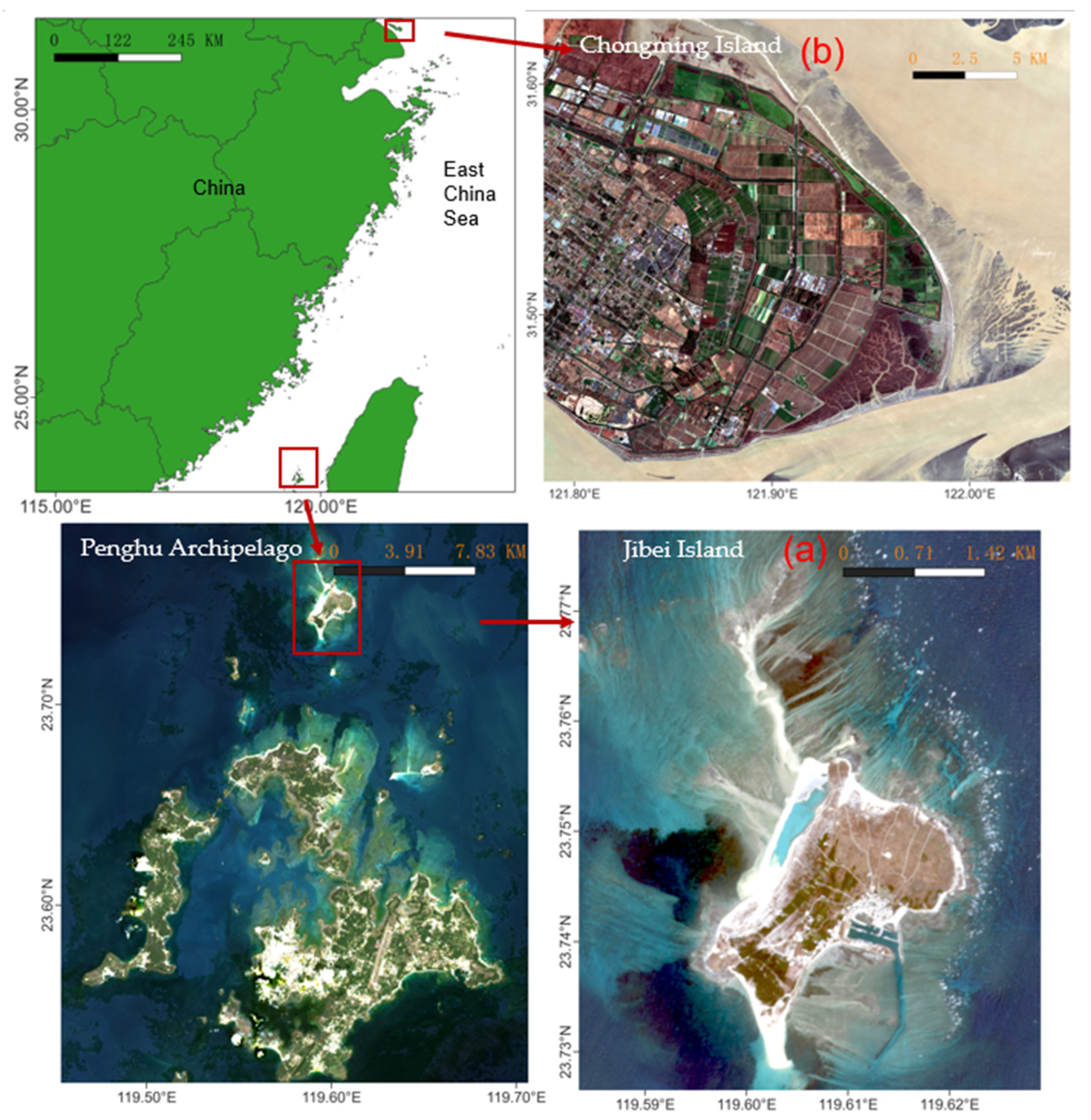
2.1. Study Area
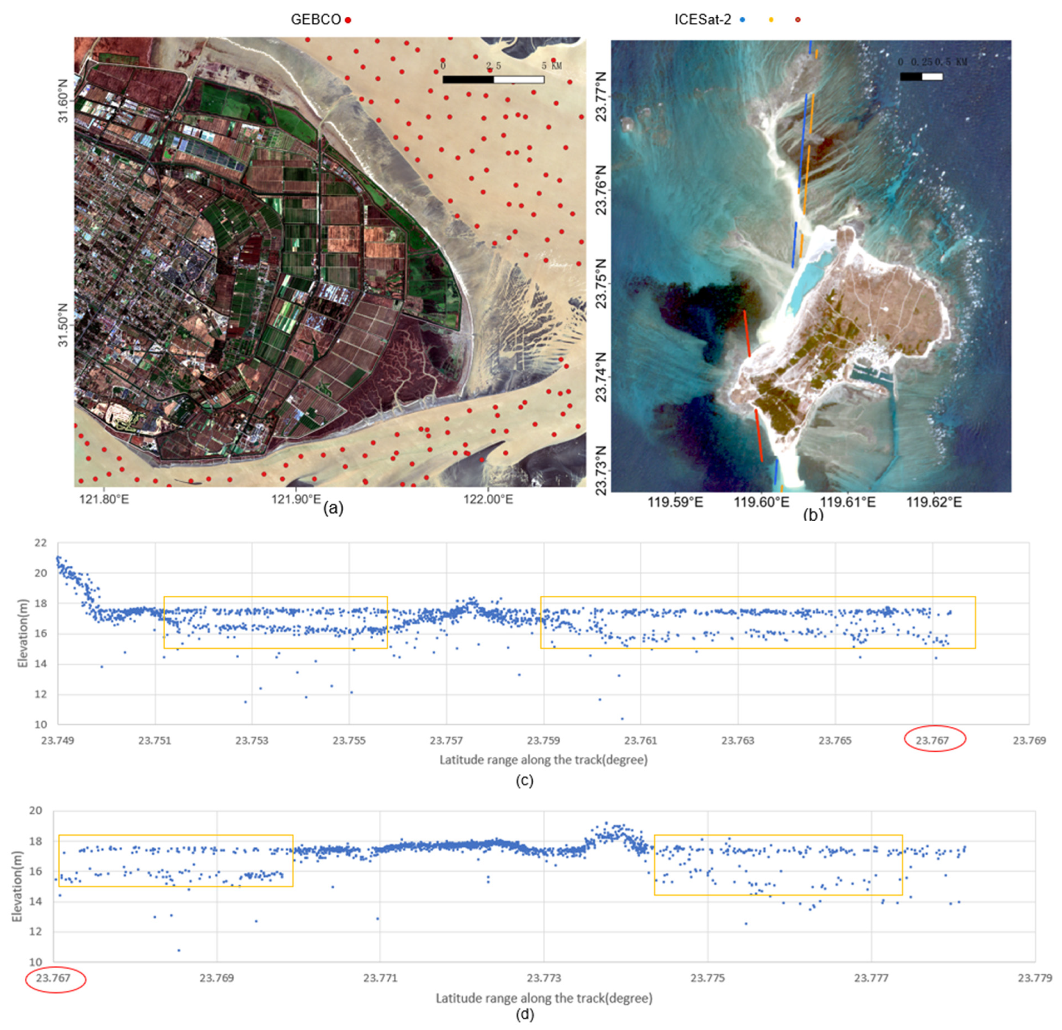
2.2. Dataset
2.3. Methods
2.3.1. NDWI
2.3.2. SVM
2.3.3. Stumpf Model
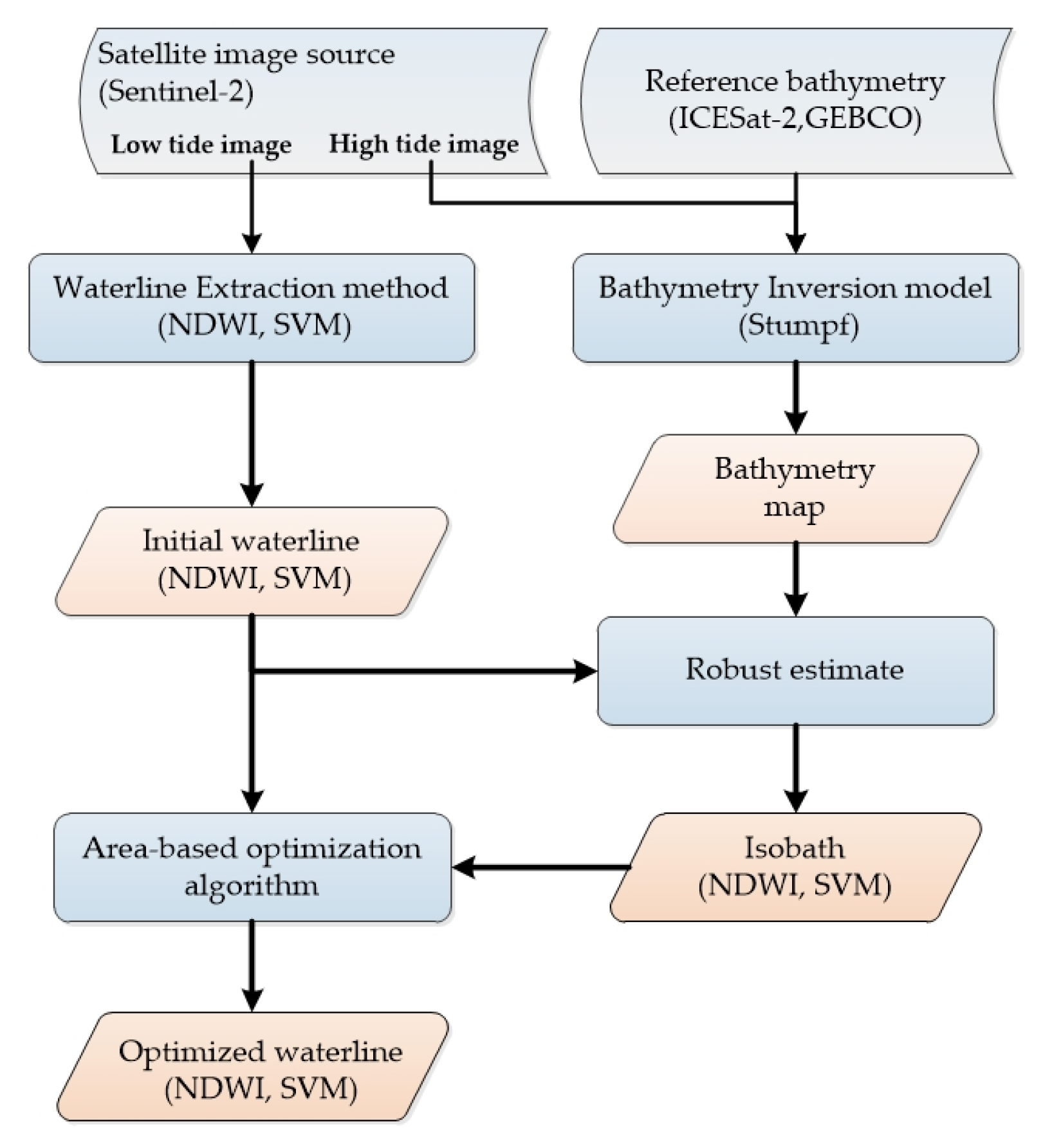
2.3.4. The Proposed Approach
- Prepare high-tide and low-tide satellite images for the targeted area;
- Obtain the bathymetry map using the high-tide image (use some reference data, such as GEBCO or ICESat-2, to obtain absolute bathymetry; relative bathymetry can still be derived if no reference data are available);
- Extract the initial waterline from low-tide images using either NDWI, SVM, or other methods;
- Extract the depth value from the bathymetry map for sample points on the initial waterline and apply robust estimate techniques to estimate the isobath (the contour line, all points on the contour line have the same elevation or depth), which best matches the initial waterline;
- If the isobath is regarded as the waterline, the process can be ended. Otherwise, the isobath is used to optimize the initial waterline;
- Form two trajectories: one trajectory is the isobath (from above Step 4), and another trajectory is the initial waterline (Step 3). Apply the proposed area-based optimization algorithm to minimize the area of differences in the above two trajectories. The optimized waterline acts as the final waterline.
Bathymetry Inversion
Isobath Estimate
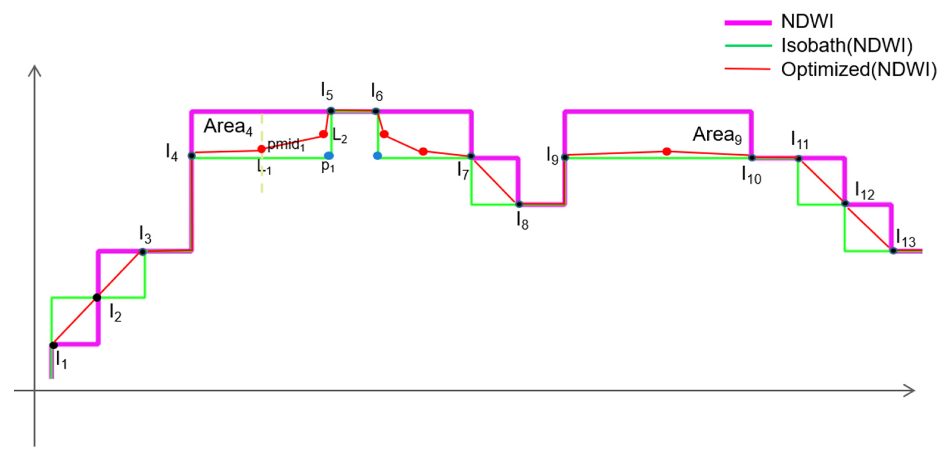
Waterline Optimization
- Split the isobath line into line segments; split the average area according to the number of line segments. The intersection isobath line could be split into N line segments according to the turning point of the raster (blue point ). For example, can be split into 2 segments, and ; each line segment is . According to the proportion of each segment to the total length, the average area is divided into N parts, as shown in Equation (4);
- Find a point on the vertical line of the line segment , such as the red point in Figure 5; this point is in the intersection area of the two lines, and the area enclosed by this point and the line segment is ;
- The curve formed by connecting all the relocation points is the recorrected waterline.
2.4. Experimental Design
2.5. Evaluation
3. Results
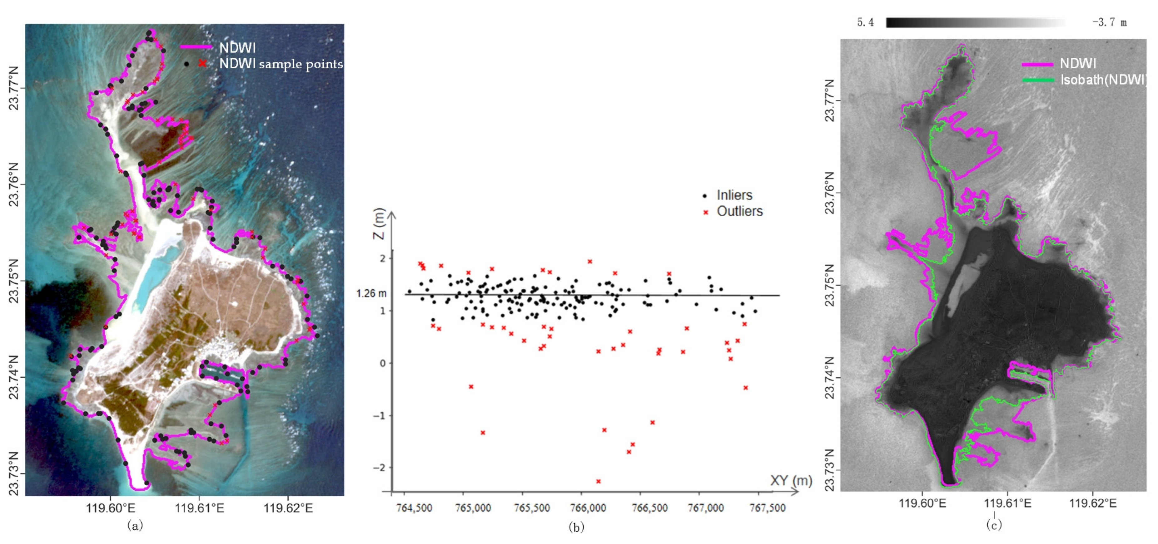
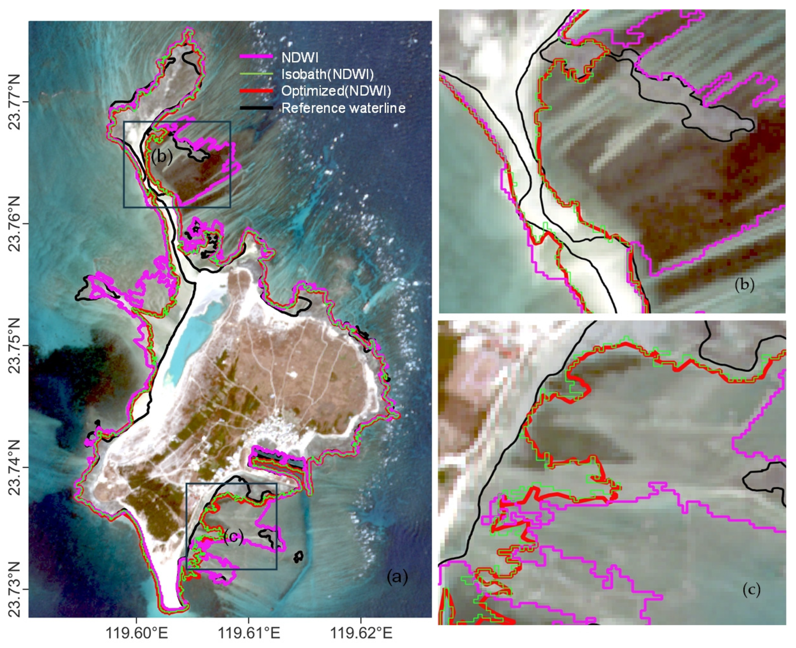
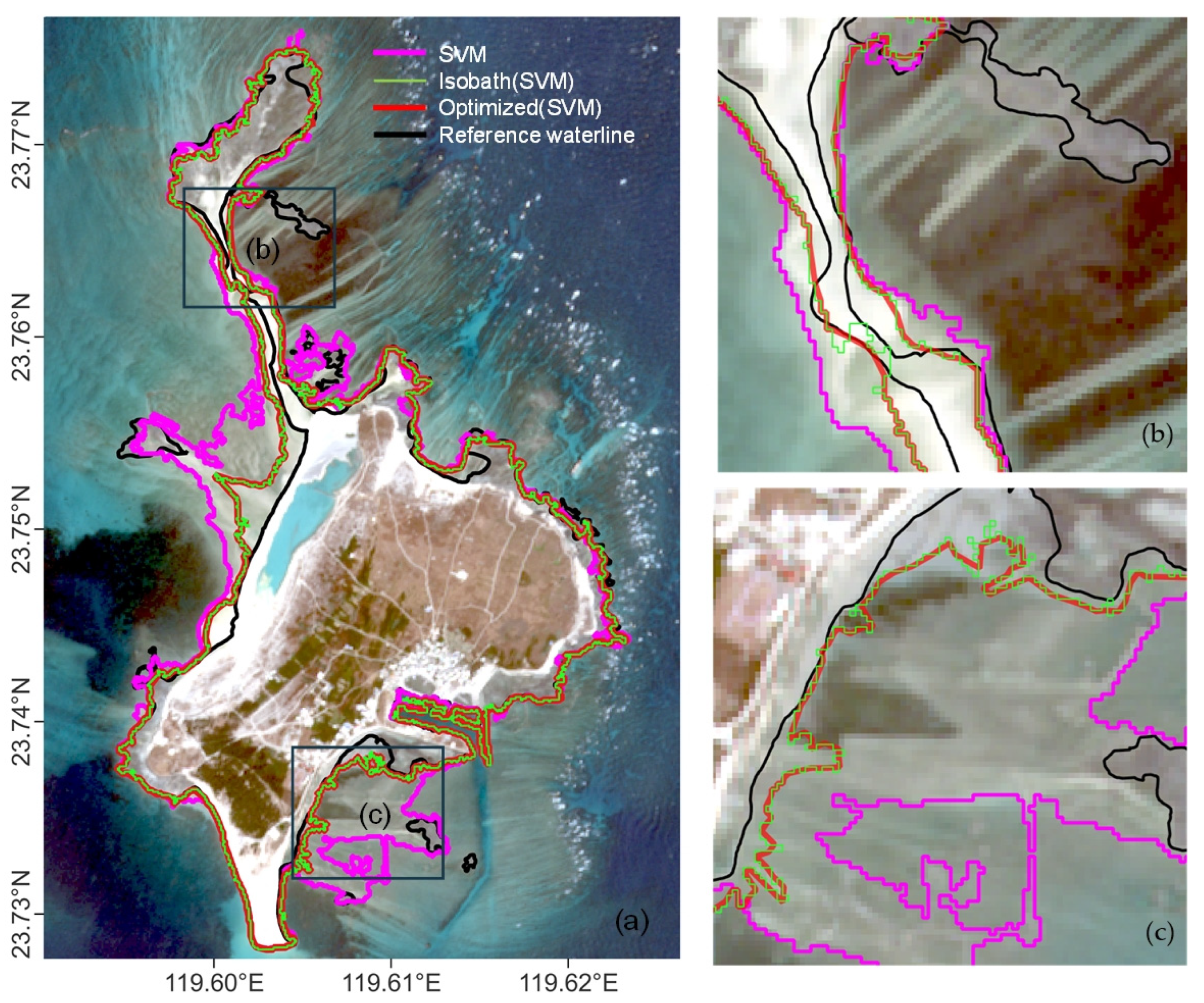
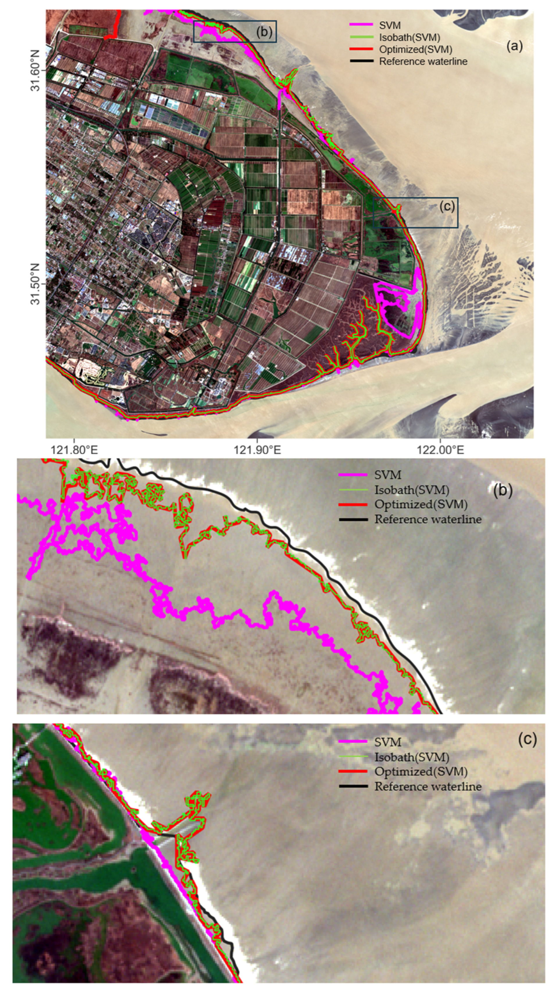
3.1. Jibei Island Waterline Extraction
- NDWI: the initial waterline was extracted using the NDWI method;
- SVM: the initial waterline extracted using the SVM method;
- Isobath (NDWI): the corresponding isobath of the initial NDWI waterline from the bathymetry map;
- Isobath (SVM): the corresponding isobath of the initial SVM waterline from the bathymetry map;
- Optimized (NDWI): the final waterline after optimizing the initial NDWI waterline and isobath (NDWI) using the area-based optimization algorithm;
- Optimized (SVM): the final waterline after optimizing the initial NDWI waterline and isobath (SVM) using the area-based optimization algorithm.
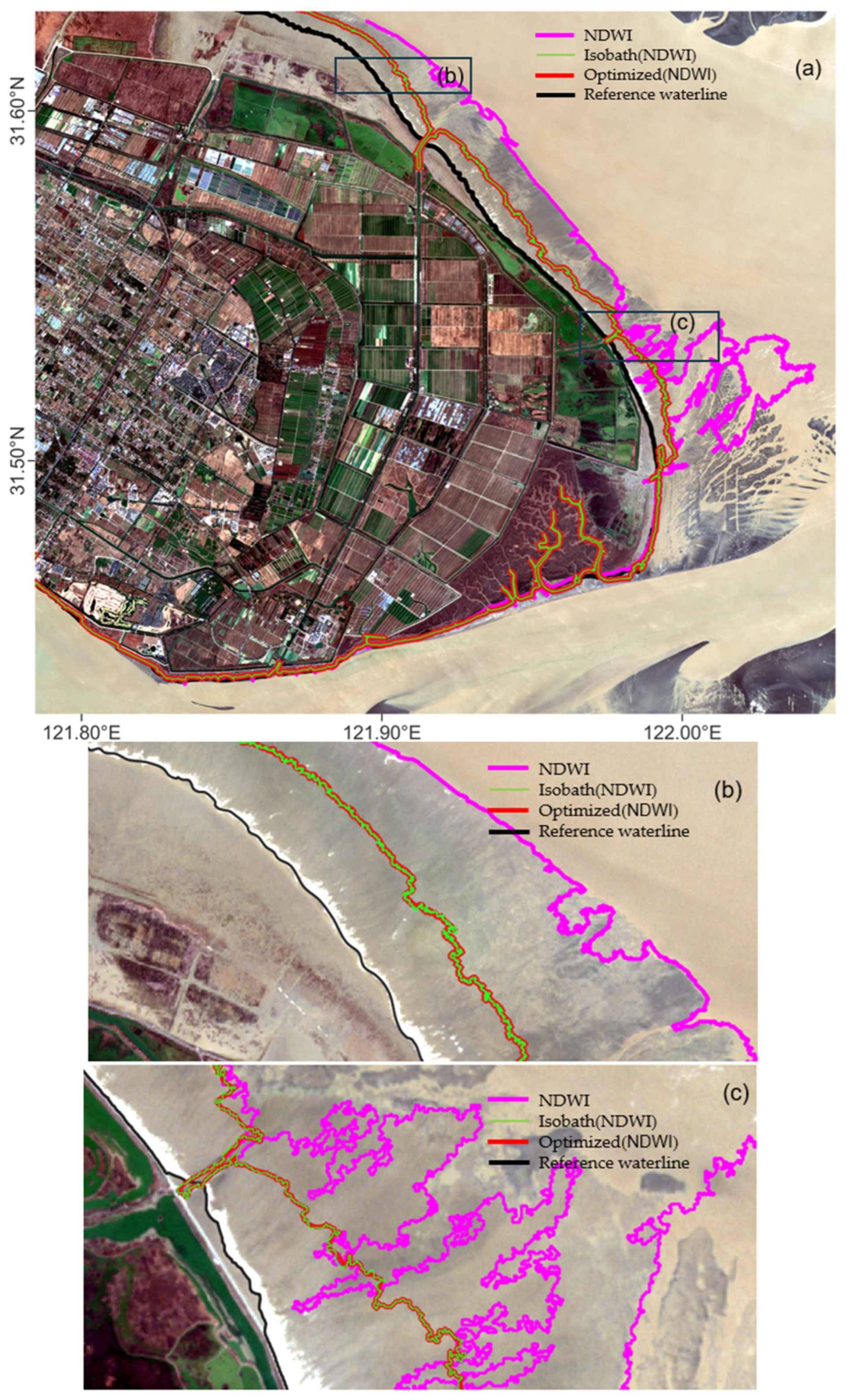
3.2. Chongming Island Waterline Extraction
4. Discussion
5. Conclusions
Author Contributions
Funding
Data Availability Statement
Acknowledgments
Conflicts of Interest
References
- Chinese Government Network. Main Data Bulletin of the Third National Land Survey [EB/OL]. 2021. Available online: https://www.gov.cn/xinwen/2021-08/26/content_5633490.htm (accessed on 25 December 2023).
- Vousdoukas, M.I.; Ranasinghe, R.; Mentaschi, L.; Plomaritis, T.A.; Athanasiou, P.; Luijendijk, A.; Feyen, L. Sandy coastlines under threat of erosion. Nat. Clim. Chang. 2020, 10, 260–263. [Google Scholar] [CrossRef]
- Almeida, L.P.; Oliveira, I.; Lyra, R.; Dazzi, R.; Martins, V.; Klein, A. Coastal Analyst System from Space Imagery Engine (CASSIE): Shoreline management module. Environ. Model. Softw. 2021, 140, 105033. [Google Scholar] [CrossRef]
- Boak, E.H.; Turner, I.L. Shoreline Definition and Detection: A Review. J. Coast. Res. 2005, 21, 688–703. [Google Scholar] [CrossRef]
- Henderson, S.; Bowen, A. Observations of surf beat forcing and dissipation. J. Geophys. Res. 2002, 107, 14-1–14-10. [Google Scholar] [CrossRef]
- Smith, S.D. Coefficients for sea surface wind stress, heat flux, and wind profiles as a function of wind speed and temperature. J. Geophys. Res. 1988, 93, 15467–15472. [Google Scholar] [CrossRef]
- Lee, J.-S.; Jurkevich, I. Coastline Detection And Tracing In SAR Images. IEEE Trans. Geosci. Remote Sens. 1990, 28, 662–668. [Google Scholar] [CrossRef]
- Appeaning Addo, K.; Walkden, M.; Mills, J.P. Detection, measurement and prediction of shoreline recession in Accra, Ghana. ISPRS J. Photogramm. Remote Sens. 2008, 63, 543–558. [Google Scholar] [CrossRef]
- Barnard, P.L.; Short, A.D.; Harley, M.D.; Splinter, K.D.; Vitousek, S.; Turner, I.L.; Allan, J.; Banno, M.; Bryan, K.R.; Doria, A.; et al. Coastal vulnerability across the Pacific dominated by El Niño/Southern Oscillation. Nat. Geosci. 2015, 8, 801–807. [Google Scholar] [CrossRef]
- Turner, I.L.; Harley, M.D.; Short, A.D.; Simmons, J.A.; Bracs, M.A.; Phillips, M.S.; Splinter, K.D. A multi-decade dataset of monthly beach profile surveys and inshore wave forcing at Narrabeen, Australia. Sci. Data 2016, 3, 160024. [Google Scholar] [CrossRef]
- Gens, R. Remote sensing of coastlines: Detection, extraction and monitoring. Int. J. Remote Sens. 2010, 31, 1819–1836. [Google Scholar] [CrossRef]
- Bouchahma, M.; Yan, W. Monitoring shoreline change on Djerba Island using GIS and multi-temporal satellite data. Arab. J. Geosci. 2014, 7, 3705–3713. [Google Scholar] [CrossRef]
- Chen, W.-W.; Chang, H.-K. Estimation of shoreline position and change from satellite images considering tidal variation. Estuar. Coast. Shelf Sci. 2009, 84, 54–60. [Google Scholar] [CrossRef]
- Sparavigna, A.C. A Study of Moving Sand Dunes by Means of Satellite Images. Int. J. Sci. 2013, 2, 33–42. [Google Scholar] [CrossRef]
- McFeeters, S.K. The use of the Normalized Difference Water Index (NDWI) in the delineation of open water features. Int. J. Remote Sens. 1996, 17, 1425–1432. [Google Scholar] [CrossRef]
- Gao, B.C. NDWI—A normalized difference water index for remote sensing of vegetation liquid water from space. Remote Sens. Environ. 1996, 58, 257–266. [Google Scholar] [CrossRef]
- Otsu, N. A threshold selection method from gray level histograms. IEEE Trans. Syst. Man Cybern. 1979, 9, 62–66. [Google Scholar] [CrossRef]
- Bayram, B.; Erdem, F.; Akpinar, B.; Ince, A.; Bozkurt, S.; Çatal, H.; Seker, D. The efficiency of random forest method for shoreline extraction from Landsat-8 and GOKTURK-2 imageries. ISPRS Ann. Photogramm. Remote Sens. Spat. Inf. Sci. 2017, IV-4/W4, 141–145. [Google Scholar] [CrossRef]
- Changda, L.; Li, J.; Tang, Q.; Qi, J.; Zhou, X. Classifying the Nunivak Island Coastline Using the Random Forest Integration of the Sentinel-2 and ICESat-2 Data. Land 2022, 11, 240. [Google Scholar] [CrossRef]
- Tsiakos, C.-A.D.; Chalkias, C. Use of Machine Learning and Remote Sensing Techniques for Shoreline Monitoring: A Review of Recent Literature. Appl. Sci. 2023, 13, 3268. [Google Scholar] [CrossRef]
- Sarp, G.; Ozcelik, M. Water body extraction and change detection using time series: A case study of Lake Burdur, Turkey. J. Taibah Univ. Sci. 2017, 11, 381–391. [Google Scholar] [CrossRef]
- Kumar, L.; Afzal, M.S.; Afzal, M.M. Mapping shoreline change using machine learning: A case study from the eastern Indian coast. Acta Geophys. 2020, 68, 1127–1143. [Google Scholar] [CrossRef]
- Hannv, Z.; Qigang, J.; Jiang, X. Coastline Extraction Using Support Vector Machine from Remote Sensing Image. J. Multimed. 2013, 8, 175–182. [Google Scholar] [CrossRef]
- Soumia, B.; Simona, N.; Mustapha Kamel, M.; Rabah, B.; Ali, R.; Walid, R.; Katia, A. Machine learning and shoreline monitoring using optical satellite images: Case study of the Mostaganem shoreline, Algeria. J. Appl. Remote Sens. 2021, 15, 026509. [Google Scholar] [CrossRef]
- Mahapatra, M.; Ratheesh, R.; Rajawat, A.S. Shoreline Change Analysis along the Coast of South Gujarat, India, Using Digital Shoreline Analysis System. J. Indian Soc. Remote Sens. 2014, 42, 869–876. [Google Scholar] [CrossRef]
- Ciritci, D.; Türk, T. Assessment of the Kalman filter-based future shoreline prediction method. Int. J. Environ. Sci. Technol. 2020, 17, 3801–3816. [Google Scholar] [CrossRef]
- Badrinarayanan, V.; Kendall, A.; Cipolla, R. SegNet: A Deep Convolutional Encoder-Decoder Architecture for Image Segmentation. IEEE Trans. Pattern Anal. Mach. Intell. 2017, 39, 2481–2495. [Google Scholar] [CrossRef] [PubMed]
- Wang, Z.; Guo, J.; Huang, W.; Zhang, S. High-resolution remote sensing image semantic segmentation based on a deep feature aggregation network. Meas. Sci. Technol. 2021, 32, 095002. [Google Scholar] [CrossRef]
- Chen, S.; Liu, Y.; Zhang, C. Water-Body Segmentation for Multi-Spectral Remote Sensing Images by Feature Pyramid Enhancement and Pixel Pair Matching. Int. J. Remote Sens. 2021, 42, 5029–5047. [Google Scholar] [CrossRef]
- Souto-Ceccon, P.; Simarro, G.; Ciavola, P.; Taramelli, A.; Armaroli, C. Shoreline Detection from PRISMA Hyperspectral Remotely-Sensed Images. Remote Sens. 2023, 15, 2117. [Google Scholar] [CrossRef]
- Xie, H.; Luo, X.; Xu, X.; Haiyan, P.; Tong, X. Automated Subpixel Surface Water Mapping from Heterogeneous Urban Environments Using Landsat 8 OLI Imagery. Remote Sens. 2016, 8, 584. [Google Scholar] [CrossRef]
- Vos, K.; Splinter, K.; Harley, M.; Simmons, J.; Turner, I. CoastSat: A Google Earth Engine-enabled Python toolkit to extract shorelines from publicly available satellite imagery. Environ. Model. Softw. 2019, 122, 104528. [Google Scholar] [CrossRef]
- Nikolakopoulos, K.; Kyriou, A.; Koukouvelas, I.; Zygouri, V.; Apostolopoulos, D. Combination of Aerial, Satellite, and UAV Photogrammetry for Mapping the Diachronic Coastline Evolution: The Case of Lefkada Island. ISPRS Int. J. Geo-Inf. 2019, 8, 489. [Google Scholar] [CrossRef]
- Nikolakopoulos, K.; Kozarski, D.; Kogkas, S. Coastal areas mapping using UAV photogrammetry. In Earth Resources and Environmental Remote Sensing/GIS Applications VIII; SPIE: Washington, DC, USA, 2017; p. 23. [Google Scholar]
- Turner, I.; Harley, M.; Drummond, C. UAVs for coastal surveying. Coast. Eng. 2016, 114, 19–24. [Google Scholar] [CrossRef]
- Chen, B.; Yang, Y.; Wen, H.; Ruan, H.; Zhou, Z.; Luo, K.; Zhong, F. High-resolution monitoring of-Beach topography and its change using unmanned aerial vehicle imagery. Ocean Coast. Manag. 2018, 160, 103–116. [Google Scholar] [CrossRef]
- Al_Fugara, A.K.; Billa, L.; Pradhan, B. Semi-automated procedures for shoreline extraction using single RADARSAT-1 SAR image. Estuar. Coast. Shelf Sci. J. 2011, 95, 395–400. [Google Scholar] [CrossRef]
- Wei, X.; Zheng, W.; Xi, C.; Shang, S. Shoreline Extraction in SAR Image Based on Advanced Geometric Active Contour Model. Remote Sens. 2021, 13, 642. [Google Scholar] [CrossRef]
- Demir, N.; Bayram, B.; Şeker, D.Z.; Oy, S.; İnce, A.; Bozkurt, S. Advanced Lake Shoreline Extraction Approach by Integration of SAR Image and LIDAR Data. Mar. Geod. 2019, 42, 166–185. [Google Scholar] [CrossRef]
- Ferrentino, E.; Nunziata, F.; Migliaccio, M. Full-polarimetric SAR measurements for coastline extraction and coastal area classification. Int. J. Remote Sens. 2017, 38, 7405–7421. [Google Scholar] [CrossRef]
- Wu, L.; Inazu, D.; Ikeya, T.; Okayasu, A. Simultaneous Observation of a Sandy Coast Based on UAV and Satellite X-band SAR. J. Jpn. Soc. Civ. Eng. Ser. B2 2022, 78, I_1051–I_1056. [Google Scholar] [CrossRef]
- Wang, J.; Wang, L.; Feng, S.; Peng, B.; Huang, L.; Fatholahi, S.N.; Tang, L.; Li, J. An Overview of Shoreline Mapping by Using Airborne LiDAR. Remote Sens. 2023, 15, 253. [Google Scholar] [CrossRef]
- Yang, L.; Li, M.; Li, J.; Jiang, Y.; Yang, H. Multiscale Spatial Relation Extraction of a Remotely Sensed Waterline in a Muddy Coastal Zone with Chongming Dongtan as AN Example. ISPRS Ann. Photogramm. Remote Sens. Spat. Inf. Sci. 2022, V-3-2022, 69–76. [Google Scholar] [CrossRef]
- Chunpeng, C.; Tian, B.; Wu, W.; Yuanqiang, D.; Zhou, Y.; Zhang, C. UAV Photogrammetry in Intertidal Mudflats: Accuracy, Efficiency, and Potential for Integration with Satellite Imagery. Remote Sens. 2023, 15, 1814. [Google Scholar] [CrossRef]
- Bergsma, E.; Almar, R. Coastal coverage of ESA’ Sentinel 2 mission. Adv. Space Res. 2020, 65, 2636–2644. [Google Scholar] [CrossRef]
- Bae, S.; Magruder, L.; Smith, N.; Schutz, B. ICESat-2 Algorithm Theoretical Basis Document for Precision Pointing Determination; ICESat-2-SIPS-SPEC-1595; NASA: Washington, DC, USA, 2018. [CrossRef]
- Stumpf, R.P.; Holderied, K.; Sinclair, M.J.L. Determination of water depth with high resolution satellite imagery over variable bottom types. Limnol. Oceanogr. 2003, 48, 547–556. [Google Scholar] [CrossRef]
- Tang, K.; Mahmud, M. Imagery-Derived Bathymetry In Strait Of Johor’s Turbid Waters Using Multispectral Images. Int. Arch. Photogramm. Remote Sens. Spat. Inf. Sci. 2018, XLII-4/W9, 139–145. [Google Scholar] [CrossRef]
- Lyzenga, D.R. Shallow-water Bathymetry Using Combined Lidar and Passive Multispectral Scanner Data. Int. J. Remote Sens. 2010, 6, 115–125. [Google Scholar] [CrossRef]
- Fotheringham, A.S.; Charlton, M.E.; Brunsdon, C. Geographically Weighted Regression: A Natural Evolution of the Expansion Method for Spatial Data Analysis. Environ. Plan. A 1998, 30, 1905–1927. [Google Scholar] [CrossRef]
- Casal, G.; Harris, P.; Monteys, X.; Hedley, J.; Cahalane, C.; McCarthy, T. Understanding Satellite-derived Bathymetry Using Sentinel 2 Imagery and Spatial Prediction Models. GIScience Remote Sens. 2019, 57, 271–286. [Google Scholar] [CrossRef]
- Ram, A.; Sunita, J.; Jalal, A.; Manoj, K. A Density Based Algorithm for Discovering Density Varied Clusters in Large Spatial Databases. Int. J. Comput. Appl. 2010, 3, 1–4. [Google Scholar] [CrossRef]
- Fischler, M.; Bolles, R. Random Sample Consensus: A Paradigm for Model Fitting with Applications To Image Analysis and Automated Cartography. Commun. ACM 1981, 24, 381–395. [Google Scholar] [CrossRef]
- Pelekis, N.; Kopanakis, I.; Ntoutsi, I.; Marketos, G.; Theodoridis, Y. Mining trajectory databases via a suite of distance operators. In Proceedings of the 2007 IEEE 23rd International Conference on Data Engineering Workshop, Istanbul, Turke, 17–20 April 2007; pp. 575–584. [Google Scholar]


| Study Area | Data Source | Date | Time (UTC) | Tide Status |
|---|---|---|---|---|
| Jibei Island | Sentinel-2 | 20210316 | 022551 | high tide |
| 20211111 | 022931 | low tide | ||
| ICESat-2 | 20191005 | 142530 | low tide | |
| 20210402 | 122421 | low tide | ||
| 20211110 | 140101 | low tide | ||
| Chongming Island | Sentinel-2 | 20230515 | 022531 | high tide |
| 20230128 | 023951 | low tide | ||
| GEBCO | 20220529 | 121058 | low tide |
| Waterline | Mean (m) | STD (m) |
|---|---|---|
| NDWI | 38.35 | 62.24 |
| SVM | 25.23 | 29.66 |
| Isobath (NDWI) | 14.85 | 16.05 |
| Isobath (SVM) | 14.56 | 15.59 |
| Optimized (NDWI) | 15.01 | 16.51 |
| Optimized (SVM) | 14.78 | 16.03 |
| Waterline | Mean (m) | STD (m) |
|---|---|---|
| NDWI | 95.57 | 62.24 |
| SVM | 30.36 | 25.90 |
| Isobath (NDWI) | 26.54 | 20.87 |
| Isobath (SVM) | 19.05 | 17.92 |
| Optimized (NDWI) | 27.34 | 21.15 |
| Optimized (SVM) | 18.93 | 17.51 |
Disclaimer/Publisher’s Note: The statements, opinions and data contained in all publications are solely those of the individual author(s) and contributor(s) and not of MDPI and/or the editor(s). MDPI and/or the editor(s) disclaim responsibility for any injury to people or property resulting from any ideas, methods, instructions or products referred to in the content. |
© 2024 by the authors. Licensee MDPI, Basel, Switzerland. This article is an open access article distributed under the terms and conditions of the Creative Commons Attribution (CC BY) license (https://creativecommons.org/licenses/by/4.0/).
Share and Cite
Yang, H.; Chen, M.; Xi, X.; Wang, Y. A Novel Approach for Instantaneous Waterline Extraction for Tidal Flats. Remote Sens. 2024, 16, 413. https://doi.org/10.3390/rs16020413
Yang H, Chen M, Xi X, Wang Y. A Novel Approach for Instantaneous Waterline Extraction for Tidal Flats. Remote Sensing. 2024; 16(2):413. https://doi.org/10.3390/rs16020413
Chicago/Turabian StyleYang, Hua, Ming Chen, Xiaotao Xi, and Yingxi Wang. 2024. "A Novel Approach for Instantaneous Waterline Extraction for Tidal Flats" Remote Sensing 16, no. 2: 413. https://doi.org/10.3390/rs16020413