Article

Development and Evaluation of a Cloud-Gap-Filled MODIS Normalized Difference Snow Index Product over High Mountain Asia

1
National-Local Joint Engineering Laboratory of Geo-Spatial Information Technology, Hunan University of Science and Technology, Xiangtan 411201, China
2
School of Geography and Information Engineering, China University of Geosciences, Wuhan 430074, China
3
School of Civil Engineering, Sun Yat-sen University, Zhuhai 519082, China
4
Key Laboratory of Remote Sensing of Gansu Province, Northwest Institute of Eco-Environment and Resources, Chinese Academy of Sciences, Lanzhou 730000, China
*
Author to whom correspondence should be addressed.
Remote Sens. 2024, 16(1), 192; https://doi.org/10.3390/rs16010192
Submission received: 8 November 2023 / Revised: 20 December 2023 / Accepted: 30 December 2023 / Published: 2 January 2024

Abstract

:
Accurate snow cover data are critical for understanding the Earth’s climate system, and exploring hydrological processes and regional water resource management over High Mountain Asia (HMA). However, satellite-based remote sensing observations of snow cover have inevitable data gaps originating from cloud cover, sensor, orbital limitations and other factors. Here an effective cloud-gap-filled (CGF) method was developed to fully fill the data gaps in Moderate Resolution Imaging Spectroradiometer (MODIS) normalized difference snow index (NDSI) product. The CGF method combines the respective strengths of the cubic spline interpolation method and the spatio-temporal weighted method for generating the CGF Terra-Aqua MODIS NDSI product over HMA from 2000 to 2021. Based on the validation results of in situ snow-depth observations, the CGF NDSI product achieves a high range overall accuracy (OA) of 93.54–98.08%, a low range underestimation error (MU) of 0.15–3.49% and an acceptable range overestimation error (MO) of 0.84–5.77%. Based on the validation results of high-resolution Landsat images, this product achieves the OA of 88.52–92.40%, the omission error (OE) of 1.42–10.28% and the commission error (CE) of 5.97–17.58%. The CGF MODIS NDSI product can provide scientific support for eco-environment sustainable management in the high mountain region.

1. Introduction

Snow cover has been identified as an essential geophysical parameter for understanding the Earth’s climate system, covering about 40% to 50% of the Northern Hemisphere during winter [1,2,3]. Snow cover exerts a strong control on the surface energy budget, water cycle, primary productivity and surface gas exchange [4,5,6,7]. As a natural solid water reservoir within the cryosphere, snow cover holds a crucial role as the source of water supply, benefiting over 17% of the global population with fresh drinking water through seasonal snowmelt-driven runoff [8,9,10].
High Mountain Asia (HMA) is the largest expanse of snow cover outside of the polar regions and feeds several large rivers, often referred to as the “Earth’s third pole” and the “Water Tower of Asia” [11,12]. Since the 1970s, HMA has undergone drastic environmental changes, including the air temperature rate more than double the global average [13]. The warming climate may be accountable for accelerated melting of glaciers and snow cover over HMA and surrounding, which could have a significant impact on water supply and water security in this region. Given these concerns, it is crucial to monitor the variability of snow cover over HMA, while the long-term and highly accurate snow cover products are fundamental for snow cover research over HMA.
Compared to the limited field surveys and the sparse, uneven distribution of available snowfall observation data, satellite remote sensing data exhibit great advantages in depicting the long-term spatio-temporal patterns of snow cover in large-scale and rugged terrain regions (like HMA). The rapid development of remote sensing technology during the last decades has generated a series of snow cover products including optical-based and microwave-based (mainly derived from passive sensors) products. Microwave-based snow products (e.g., snow depth (SD) and snow water equivalent) derived from passive sensors have been proven to be useful for monitoring snow cover [14,15,16,17,18]. However, their coarse (∼25 km) footprints and the saturation of observations in deep snow (>0.8 m depth) greatly limit the applicability for mountainous areas [19,20,21]. In comparison, optical-based sensors can also provide snow cover data, in terms of more appropriate temporal and spatial resolutions by making full use of snow’s unique reflective properties in the visible and shortwave infrared bands [18,22,23,24,25]. Currently, a variety of long-time series optical-based snow cover products with different temporal and spatial resolutions have been widely used, such as Advanced Very High Resolution Radiometer (AVHRR) Global Area Coverage (GAC) daily snow cover fraction products [26], the daily Visible Infrared Imaging Radiometer Suite (VIIRS) snow cover products [27] and the Moderate Resolution Imaging Spectroradiometer (MODIS) snow cover products [28]. Among them, the daily MODIS snow cover products from the Terra (MOD10A1) and Aqua (MYD10A1) satellites are widely used to depict the spatio-temporal patterns of snow cover, due to the advantages of a long-time series (available since 2000), high spatio-temporal resolution (i.e., 500 m and daily), global coverage and being freely available. Previous studies have demonstrated that MODIS snow cover products perform well in extracting snow cover information, exhibiting an overall accuracy exceeding 90% under clear sky conditions, despite some remaining uncertainties in forest coverage and mountainous areas [25,29,30,31,32,33,34]. Nevertheless, cloud contamination in MODIS snow cover products often causes numerous data gaps, which greatly limits their applications [35,36,37].
To reduce or eliminate the effects of cloud data gaps in the MODIS snow cover products, various methods have been developed over the past decade. Traditional cloud removal algorithms can be categorized into four types: temporal, spatial, multi-source fusion and spatio-temporal combination methods [18]. In addition, these methods have mainly been aimed at binary snow cover (BSC) or fractional snow cover (FSC) data from the MODIS snow cover product Collection 5 (C5) [18]. Temporal methods include the Terra and Aqua combination (TAC) [38], adjacent temporal deduction [39,40], multi-day combination [38,41] (e.g., the 8-day composite products of MOD/MYD10A2 product), season filter [39,42] and temporal interpolation using a mathematical function [31,43,44,45]. These temporal methods utilize the instability of cloud cover and the temporal correlation of snow cover to effectively reduce cloud cover, either partially or completely, with high overall accuracy. However, they have the problems of sacrificing temporal resolution, failing to reduce the cloud cover completely and having low accuracy when cloud coverage is continuous. Spatial methods include the spatial neighborhood filter [42], the snowline mapping approach [46] and spatial interpolation based on a regression function [47]. These spatial methods utilize the spatial distribution characteristics of snow cover for reclassifying cloud pixels. However, they have the problems of high computational complexity, and having low accuracy in a region with high cloud coverage for all spatial methods. Multi-source fusion methods, including the optical/microwave observations fusion, optical/meteorological station observations fusion and optical/microwave/meteorological station observations fusion [16,48,49,50]. These multi-source fusion methods have the capability to eliminate all cloud pixels, while the accuracy depends on the complementarity and precision of the input data [18]. However, they often sacrifice spatial resolution and result in varying degrees of uncertainty. Considering all the appearing problems from the above three methods, the spatio-temporal combination methods can achieve satisfactory cloud removal effectiveness and accuracy. Spatio-temporal combination methods rely on the correlations of snow cover in space and time, typically taking two basic forms [1]. One is to take advantage of multiple spatial methods and temporal methods step by step [38,40,42,47,51]. The other is to utilize the spatial and temporal information simultaneously [52,53,54,55]. Between the two forms of methods, the latter has shown more promise in recent years because it uses spatio-temporal information from the snow cover and removes all cloud contamination in one step. For example, Li et al. [54] developed an adaptive spatio-temporal weighted method to estimate cloud pixels by considering the probability of snow cover; Hou et al. [52] introduced a gap-filling method that utilizes a non-local spatio-temporal filter method to eliminate cloud contamination for daily MODIS FSC products; Huang et al. [53] proposed a spatio-temporal model based on hidden Markov random fields that integrates spatio-temporal-spectral information along with environmental relationships. However, these methods suffer from issues related to high computational complexity and excessively high time costs.
Currently the version of MODIS snow cover product has moved from C5 to Collection 6 (C6), because the forward processing of MODIS product C5 has been discontinued in 2016. In addition, since the NDSI from C6 is a more accurate description index of the snow detection as compared to the FSC from C5 [56], more studies are shifting to the use of MODIS C6 products. Research works have demonstrated that the MODIS snow cover product C6 has high accuracy in the Tibetan Plateau, with Terra product C6 being comparable to Terra product C5, and Aqua product C6 truly having better accuracy than Aqua product C5 [57,58,59]. However, the data gaps from cloud contamination in C6 still exist, and thus a cloud removal algorithm for MODIS NDSI products is necessary. Given the advantages and disadvantages of the above cloud removal methods, we propose a cloud-gap-filled (CGF) method to retrieve the missing NDSI information beneath the cloud gaps in the MODIS NDSI product. The CGF method can effectively combine the temporal interpolation method with the spatio-temporal weighted method, leveraging their individual strengths. The ultimate goal is to develop a long-term daily cloud-free MODIS NDSI product for HMA with high precision. This product will facilitate climate and glacio-hydrological modelling and understanding of the present dynamics of the cryosphere in the region. The abbreviations for key terminology mentioned in this paper are shown in Table A1.

2. Study Area and Data
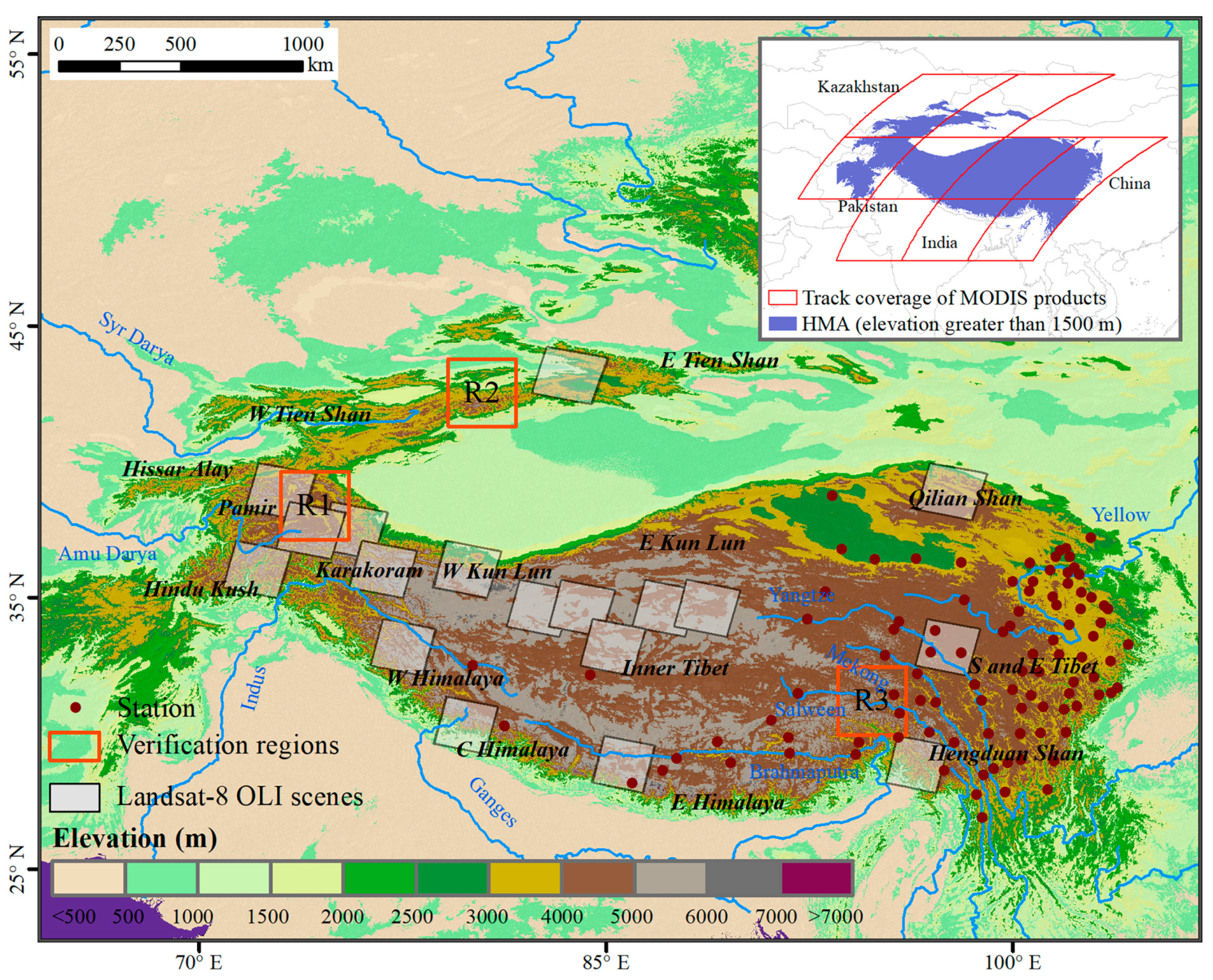
2.1. Study Area

The HMA refers to the vast high-altitude geographical area in Central Asia (spanning 22–47°N and 64–107°E), encompassing the Asian mountain ranges (e.g., Tien Shan, Pamir, Karakoram, Kunlun Mountain, and the Himalayas) surrounding the Tibetan Plateau (Figure 1). Fifteen subregions of HMA according to the Randolph Glacier Inventory version 6.0 (RGI v6.0) are shown in Figure 1 [60]. With an average elevation exceeding 4000 m, the HMA constitutes the largest expanse of snow cover outside of the Earth’s polar regions. Many rivers (e.g., Yangtze, Yellow, Indus, Brahmaputra and Syr Darya) are recharged by the abundant snow/glacier melt water in HMA and provide a major headwater for almost 2 billion people [12,61,62,63,64,65]. In addition, the HMA has typical alpine vegetation cover, mainly including alpine grassland (1.52 × 10⁶ km2), alpine meadow, temperate grassland, deciduous broad-leaved forest and forest [66]. The changes in snow cover triggered by climate change have a significant impact on terrestrial ecosystems, notably affecting the phenology of alpine vegetation [67,68].

2.2. Data

2.2.1. MODIS Snow Cover Products

The version six MODIS Terra (MOD10A1 C6) and MODIS Aqua (MYD10A1 C6) daily snow cover products from 2000 to 2021 from the National Aeronautics and Space Administration (NASA) Earthdata website (https://search.earthdata.nasa.gov/search, accessed on 10 April 2022) are used in this study, covering the whole study area with nine tiles (Figure 1). The C6 product has implemented several algorithm improvements of snow cover and replaces the BSC and FSC layers in the C5 products with two new layers: raw NDSI and NDSI snow cover. The original MODIS NDSI layer is mosaicked, resampled and converted to a geographic projection (WGS84 coordinate system, 0.005 degree resolution). After that, the pixel value in the original MYD10A1 and MOD10A1 products are reclassified into two categories: (1) valid NDSI_Snow_Cover values ranging from 0 to 100 (with values for inland water and ocean set to 0); (2) invalid cloud-gap values of 250, encompassing the original classifications for cloud, missing data, detector saturated, night and no decision.

2.2.2. Ground Snow Depth (SD) Measurements

The SD observations at 99 meteorological stations (Figure 1) from 2001 to 2013 (https://data.tpdc.ac.cn/en/data/72d6dadf-8e1c-458b-b24e-91539042dfe6/, accessed on 5 August 2022) are utilized for accuracy validation [69,70]. The released SD data have performed quality control and homogenization procedures to be a high-quality data resource.

2.2.3. Landsat OLI Satellite Images

The Landsat-8 OLI satellite images (45 scenes, Figure 1) are used to derive high-resolution BSC maps for comparison and validation of the CGF MODIS NDSI product in this study. The images with less than 30% cloud coverage are selected through the ‘CLOUD_COVER’ under clear sky and visual identification. The images are provided and processed by the Google Earth Engine platform (https://earthengine.google.com/, accessed on 12 August 2022). The detailed selected images information is shown in Table A2. All data processing is on the platform.

2.2.4. Digital Elevation Model (DEM) Data

The Shuttle Radar Topography Mission (SRTM) 90 m gridded digital elevation model (DEM) version 4.1 data are available from CGIAR Consortium for Spatial Information (CGIAR-CSI, http://srtm.csi.cgiar.org/, accessed on 13 April 2022). These data are resampled to 500 m for matching the MODIS snow cover product and used for extracting elevation information during the procedure of CGF method.

3. Methods

In this study, the implementation of the CGF method included three substeps: (1) the Terra and Aqua daily combination is executed to remove partial cloud gaps; (2) three temporal interpolation methods (TI) and a spatio-temporal weighted (STW) method are experimented for reconstructing NDSI information of cloud pixel separately; (3) the “Cloud Assumption” approach and cloud persistence days (CPD) are introduced to assess the performance of these four methods, and then the final CGF method is determined by how these four methods are combined (Section 4.1). Figure 2 presents a detailed flowchart of the proposed CGF method for MODIS NDSI product. Finally, daily CGF MODIS NDSI product is generated, and its accuracy is evaluated based on in situ SD observations and high-resolution snow cover maps derived from Landsat images.

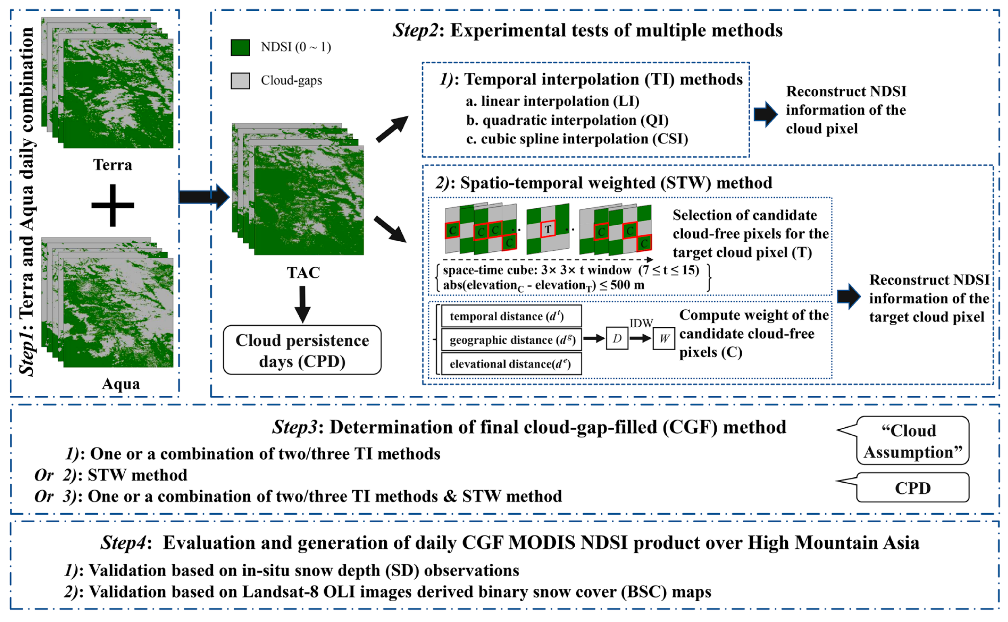
3.1. Cloud-Gap-Filled (CGF) Method

3.1.1. Terra and Aqua Daily Combination (TAC)

The TAC refers to merge MOD10A1 (Terra) and MYD10A1 (Aqua) products on the same day on a pixel-by-pixel basis, efficiently reducing the cloud gaps with negligible precision sacrifice [71]. Thus, this method is introduced as a preprocessing to reduce cloud coverage preliminarily. The complete combination rule is: (1) when a pixel is cloud-free in both MOD10A1 and MYD10A1, the combination pixel value is set to the MOD10A1 NDSI value; (2) when a pixel is cloud-free only in one of the products, the combination pixel value is set to the cloud-free NDSI value; (3) for the remaining pixels, they are identified as cloud pixels; (4) for the first 2 years only Terra was in orbit, thus the period before 4 July 2002 is only based on MOD10A1 product.

3.1.2. Temporal Interpolation (TI) Method

After TAC, there are still a large number of clouds in the MODIS NDSI products. The NDSI can offer an accurate depiction of the gradual changes in snow cover over time, due to NDSI’s ability to accurately depict the gradual changes in snow cover over time, the clouds in MODIS NDSI data can be removed through temporal interpolation filtering. Tang et al. [71] developed a cubic spline interpolation (CSI) for MODIS NDSI products, and this method effectively filled in the missing data under the cloud cover. In this study, three temporal interpolation methods: linear interpolation (LI), quadratic interpolation (QI) and CSI are used for experimental test of temporal interpolation filtering. All interpolation processes are carried out in the Interactive Data Language platform (IDL, version 8.5).

3.1.3. Spatio-Temporal Weighted (STW) Method

However, the temporal interpolation algorithm may cause some error in the case of long cloud persistence days [71]. Inspired by the work of Jing et al. [24] and Li et al. [54], this study proposes STW as the comparison with the above three temporal interpolation methods, which simultaneously takes advantage of the spatial and temporal correlations of snow cover. In the proposed approach, the NDSI information of candidate cloud-free pixels within a certain spatio-temporal window are used to reconstruct the missing NDSI information of the target cloud pixel. The implementation of STW included three substeps: (1) the spatio-temporal selection of candidate cloud-free pixels; (2) the calculation of spatio-temporal weights for candidate cloud-free pixels; (3) the calculation of NDSI values for target cloud pixel based on the spatio-temporal weights (Figure 2).
In a target TAC image, N candidate cloud-free pixels are extracted within a 3 × 3 × t (7 ≤ t ≤ 15) space-time cube, which denotes a spatial window of dimensions 3 × 3 and a time window of t days with the center of the time window corresponding to the day of data gap. A space-time cube that is too small may not provide sufficient candidate cloud-free pixels, while a space-time cube that is too large can result in increased computational and time costs during the cloud removal process [72]. Thus, the value of t depends on whether it is satisfied such that N accounts for at least 30% (this threshold has been tested to be appropriate) of the total number of pixels in the space-time cube. In addition, many studies have demonstrated that snow fraction exhibits a positive linear correlation with elevation [73,74,75]. Thus, an elevation control condition (i.e., the absolute value of the difference in elevation between the candidate cloud-free pixels and the target cloud pixel should be less than or equal to 500) is added in this study to constrain the selection of candidate cloud-free pixels.
The reconstructed NDSI information of the target cloud pixel can be expressed by Equations (1)–(5). The weight Wi decides the contribution of the candidate cloud-free pixels to reconstructing NDSI information of the target cloud pixel and is calculated by the inverse distance weighted (IDW) method. It is determined by the temporal distance, geographic distance and elevational distance between the target cloud pixel and the candidate cloud-free pixels. Shorter time intervals, smaller distance and closer elevation of the candidate cloud-free pixel to the target cloud pixel produce a higher weight (i.e., greater contribution) for the candidate cloud-free pixel.
N D S I k T = i N W i × N D S I i C where W i = ( 1 / D i ) / i N ( 1 / D i )
D i = ( d i t ) 2 + ( d i g ) 2 + ( d i e ) 2
where N D S I k T denotes the final weighted NDSI of the target cloud pixel k. N D S I i C is the preprocessed (i.e., TAC) NDSI of the candidate cloud-free pixel i. N is the number of the candidate cloud-free pixels. Wi denotes the spatio-temporal weight. Di denotes the synthetic spatio-temporal distance.
The temporal distance d i t between the target cloud pixel k and the candidate cloud-free pixel i can be calculated according to Equation (3). The unit of time is the day.
d i t = 1 + a b s ( t i m e i t i m e k ) / t w
where tw is the width of searching temporal window that is used to normalize the temporal distance.
The geographic distance d i g between the target cloud pixel ( x k , y k ) and the candidate cloud-free pixel ( x i , y j ) can be calculated according to Equation (4). The unit of horizontal or vertical distance is the number of pixels between the two pixels in horizontal or vertical direction.
d i g = 1 + ( x i x k ) 2 + ( y i y k ) 2 / g w
where gw is the width of searching geographic window (gw = 1) that is used to normalize the geographic distance.
The elevational distance d i e between the target cloud pixel k and the candidate cloud-free pixel i can be calculated according to Equation (5). The unit of elevation is meter.
d i e = 1 + a b s ( e l e v a t i o n i e l e v a t i o n k ) / e w
where ew is the width of searching elevational window (ew = 500 m) that is used to normalize the elevational distance.

3.2. Validation Method

3.2.1. Accuracy Assessment Based on “Cloud Assumption”

Utilizing the original NDSI value of the MODIS snow cover product as the validation data provides the most direct way to assess the accuracy of different TI methods and STW method in filling in cloud gaps over the entire study area. Therefore, the strategy we perform is to assume that the images on multiple random dates are cloud-covered. In addition, then we use different TI methods and STW method to reconstruct NDSI values (i.e., simulated NDSI values) for these images and subsequently compare them with the original images assumed before (i.e., reference true NDSI value). The TAC NDSI image of twenty dates (i.e., 12 February, 12 May, 13 October and 27 October of 2017; 5 February, 7 April, 31 July and 4 November of 2018; 16 February, 12 April, 12 August and 8 December of 2019; 27 March, 23 May, 17 September and 10 November of 2020; 20 March, 25 June, 26 August, 11 November of 2021) from 2017 to 2021 are selected. The performance of each method is evaluated using two metrics: mean absolute error (MAE) and root mean square error (RMSE), calculated using Equation (6) and Equation (7), respectively.
MAE = i = 1 n c i s i n
RMSE = i = 1 n c i s i 2 n
where ci and si are the simulated NDSI value and reference true NDSI value, respectively; n is the total number of reference true NDSI pixels.
In addition, we introduce the cloud persistence days (CPD) combined with MAE and RMSE to evaluate the accuracy of different reconstruction methods and determine the final CGF method. The CPD represents the number of consecutive days of cloud observed for a pixel from the last cloud-free observation to the next cloud-free observation [71]. The CPD for each cloud pixel are calculated using the daily TAC images from 2017 to 2021.

3.2.2. Validation Based on In-Situ SD Observations

The CGF MODIS NDSI product are compared with the daily SD observed by ninety-nine meteorological stations from 2001 to2013. The confusion matrix widely used [76], presented in Table 1. The ε1= 1, 2, 3 and 5 cm are the defined threshold values (referring to different measurements of SD) for the in situ SD observations. In addition, the ε2= 0.10 [57], 0.29 [58] and 0.40 [37] are the defined threshold values for the MODIS NDSI to determine whether a pixel is covered by snow.

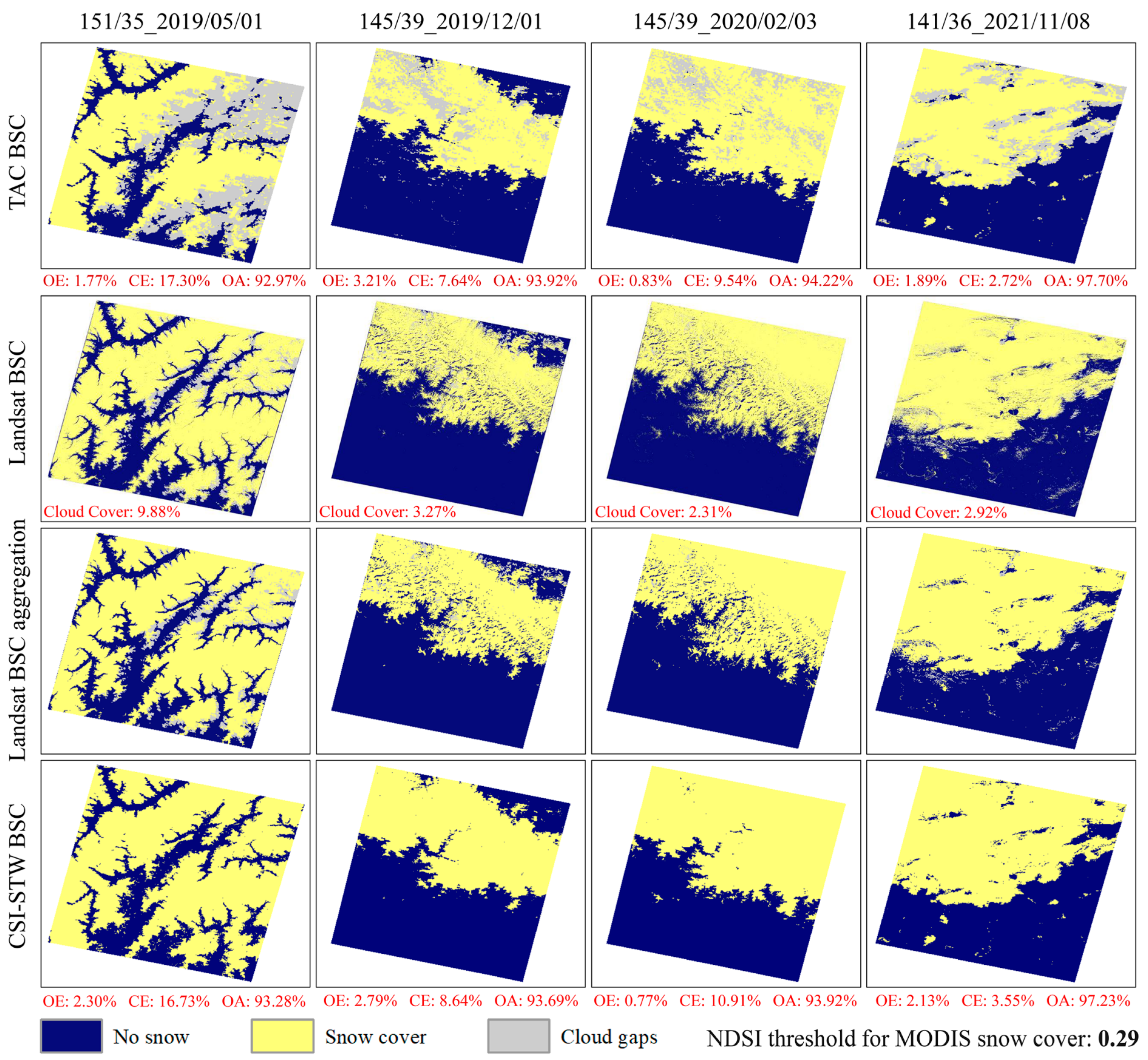
3.2.3. Validation Based on Landsat-8 OLI Images Derived BSC Maps

The BSC maps with 30 m resolution retrieved from Landsat-8 OLI images based on the Google Earth Engine platform are used to verify the CGF MODIS NDSI product in this study. The method of BSC map generation consists of two parts: the first part is the SNOMAP algorithm [2,77], which defined the NDSI of a snow pixel as greater than or equal to 0.40. Furthermore, to eliminate the influence of water bodies and other land cover, the reflectance of NIR greater than 0.11 and green band greater than 0.10 are adopted in this algorithm [78]. The second part is proposed by Wang et al. [79] and the normalized difference vegetation index (NDVI), which are introduced in this study to enhance the identification of the forest snow cover. The specific strategy is that a pixel with NDSI < 0.4, NDFSI > 0.4 and NDVI < 0.6 is identified as the snow pixel in the forest [80]. The NDSI, NDFSI and NDVI are defined as follows Equations (8)–(10):
NDSI = ρ green ρ swir ρ green + ρ swir
NDFSI = ρ nir ρ swir ρ nir + ρ swir
NDVI = ρ nir ρ red ρ nir + ρ red
where ρgreen, ρswir, ρnir and ρred correspond to the reflectance of the green, SWIR, NIR and red bands measured in Landsat imagery.
In addition, the 500 m BSC maps are aggregated from the Landsat 30 m BSC maps through 50%-pixel aggregation to match the spatial resolution of the MODIS NDSI product. The specific strategy is that if an aggregated pixel (500 m) contains more than 50% snow cover pixels (30 m) and lower than 5% cloud pixels (30 m), it is assigned to “snow covered”; otherwise, it is assigned “snow free” or “cloud” (those with >5% of the 30 m pixels flagged as “cloud” or “cloud shadow”) [58,78]. Both cloud and cloud shadow are identified using the quality assessment (QA) band of Landsat-8 OLI image. Then, the CGF MODIS NDSI derived BSC maps are evaluated with the Landsat BSC maps based on the confusion matrix including the metrics of OA, commission error (CE) and omission error (OE) (Table 2).

4. Results

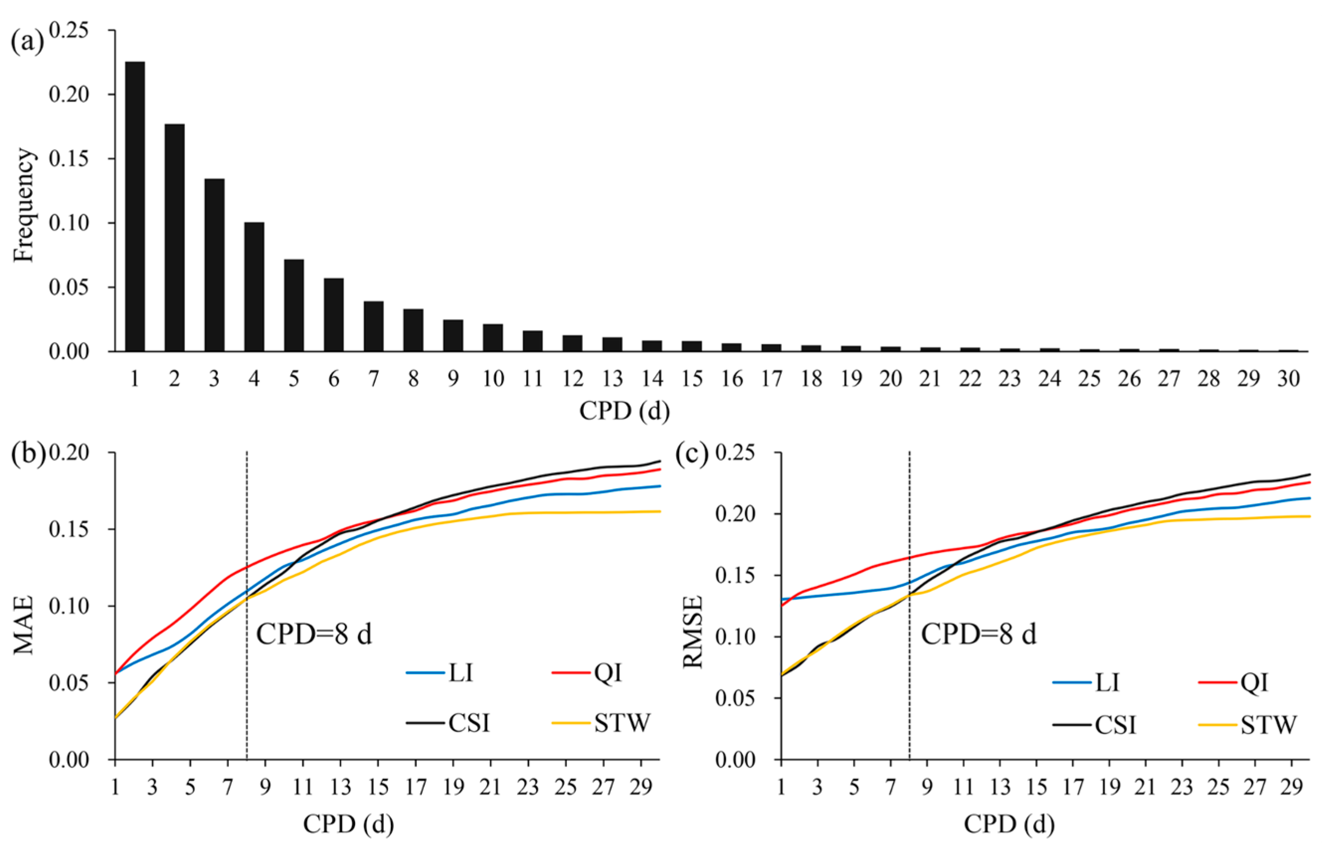
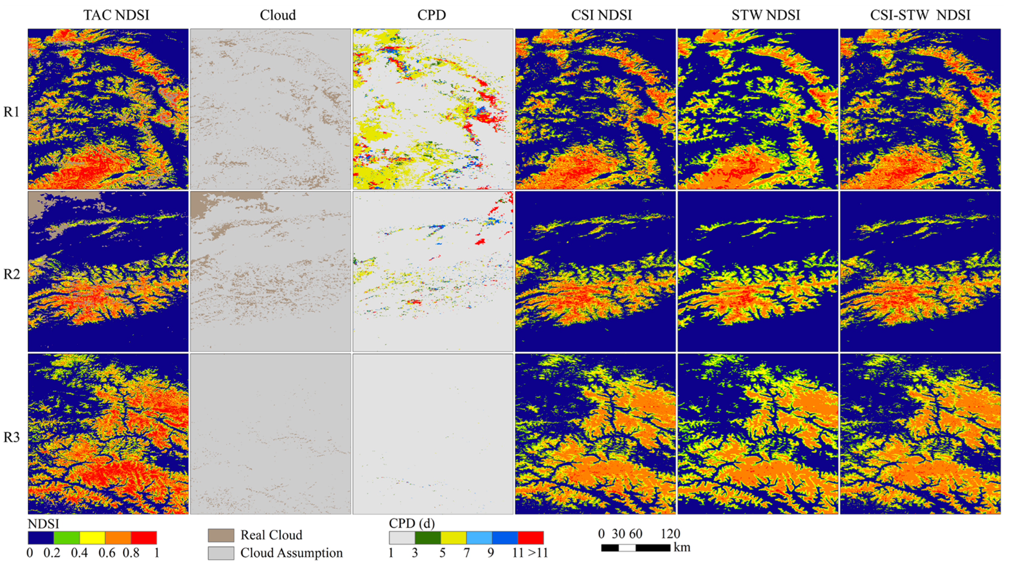
4.1. The Determination and Effectiveness of the CGF Method

As shown in Figure 3a, the frequency of the CPD reduces gradually as the increasing of CPD value, and the frequency of CPD ≤ 5 d and CPD ≤ 15 d for the cloud-covered pixels reach 70.92% and 94.07%, respectively. It can be clearly seen that the accuracy of these four methods is related to CPD with the MAE and RMSE increasing as the rising of CPD (Figure 3b,c). The accuracy of LI and QI is obviously lower than the CSI and STW due to higher values of MAE and RMSE. For the CSI method and STW method, when the CPD < 8 d, the MAE and RMSE curves of the two methods are approximately the same, i.e., a close accuracy; in the case of the CPD ≥ 8 d, the STW has the slightly higher accuracy than CSI due to the lower values of MAE and RMSE. The overall MAE/RMSE of the methods of LI, QI, CSI and STW using the frequency of CPD as the weight are 0.080/0.137, 0.088/0.144, 0.066/0.101 and 0.064/0.099, respectively.
To directly show the cloud removal results, Figure 4 shows the spatial comparison in three regions (R1, R2 and R3, Figure 1), including the TAC NDSI image, real cloud and cloud assumption image, CPD image, CSI NDSI image, STW NDSI image and the CSI-STW NDSI image. The CSI-STW image is the combination of the CSI NDSI image (when the CPD < 8 d, and the frequency of CPD is 80.53%) and STW NDSI image (when the CPD ≥ 8 d, and the frequency of CPD is 19.47%) based on the CPD NDSI image. It can be clearly seen that both CSI NDSI and STW NDSI images can generally maintain well the spatial distribution of snow cover compared with the true TAC NDSI image, and the distribution of reconstructed pixels have spatial continuity. However, there are some abrupt changes in the reconstructed pixels of the CSI NDSI image with high CPD. In addition, the reconstructed result of STW NDSI image tends to have some overestimations in low CPD region, but performs better in high CPD region than the CSI NDSI image. Therefore, the combination of the CSI and STW (i.e., CSI-STW NDSI image) is determined as the final CGF method, which can take full advantage of the respective precision advantages and spatial accuracies of CSI and STW NDSI (Figure 4, column 6). Moreover, this combination ensures high efficiency, due to higher time cost (high computational complexity) for STW. The CPD threshold (CPD = 8 d) for the combination is taken from the accuracy results in Figure 3.

4.2. The Accuracy of the CGF MODIS NDSI Product

4.2.1. Validation Based on In Situ SD Observations

The in situ SD observations are used as the ground truth to verify the snow classification accuracy of the TAC NDSI and CSI-STW NDSI datasets (Table 3). For different threshold combinations of ε1 and ε2, the OAs, MUs and MOs obtained by the CSI-STW NDSI compared with the TAC NDSI show satisfactory performance. The CSI-STW NDSI efficiently captures the snow cover referring to the in situ measurements, with an average OA of more than 95%. However, the TAC NDSI is insufficient to accurately detect the snow cover, with an average OA of only 60.45%. Note: The reason for the significant difference in OA between TAC NDSI and CSI-STW NDSI is that the calculation of OA is considering the case where TAC is cloud-covered when station records SD (e and f in Table 1). Although the MU and MO of the CSI-STW NDSI are slightly higher than the TAC NDSI, they are still within an acceptable range. To sum up, the CGF method proposed in this study can fill all of the data-gap pixels, capture more snow events and restore the snow cover information with a high reliability.

4.2.2. Validation Based on High-Resolution BSC Maps

In the absence of meteorological station data, a good way to evaluate the accuracy of the CGF MODIS NDSI product is to compare it with snow cover maps derived from higher-resolution sensors. In this study, a total of 45 Landsat-8 images (Figure 1, Table A2) with different snow coverages from January 2017 to December 2021 are selected for this accuracy validation. As shown in Table 4, the OA of TAC NDSI is 88.86–93.11% for different MODIS NDSI thresholds. Based on the CGF method, the data gaps are filled very effectively, with the OA of CSI-STW NDSI (88.52–92.40%) slightly lower than TAC NDSI (with less loss of accuracy). Table 5 further presents the validation results of CSI-STW NDSI for filling the data-gap pixels in the TAC NDSI dataset, based on the Landsat-8 BSC maps under clear-sky conditions. The OA of CSI-STW NDSI for data-gap pixels in TAC NDSI is 86.23–88.41% for different MODIS NDSI thresholds, which is 2.63–6.08% slightly lower than TAC NDSI (gap-free pixels) in Table 4. The results from Table 4 and Table 5 demonstrate that the CGF method proposed in this study can develop more reliable snow cover products, with high OA and acceptable OE and CE. In addition, the MODIS NDSI threshold is an important factor affecting the accuracy of MODIS snow cover mapping. The OA tends to increase, the CE tends to decrease and the OE tends to increase as NDSI threshold increases. However, the NDSI threshold of 0.29 notably improves the detection of snow cover and achieve outstanding OE and CE, compared to the other two thresholds. It can be concluded that the NDSI threshold of 0.29 is the best threshold to describe the spatial pattern of snow cover of HMA when using MODIS snow-cover data, which is coherent with the conclusion of Zhang et al. [58]. Figure 5 shows the snow cover mapping results, i.e., TAC BSC, Landsat BSC, Landsat BSC aggregation and CSI-STW BSC, correspond to four Landsat scenes to facilitate the analysis of their spatial consistency. In addition, the MODIS NDSI threshold is set to 0.29. It can be seen that the spatial distribution of CSI-STW BSC is fairly consistent with Landsat BSC, with notably improvement in the detection of snow cover information compared to the TAC BSC. Overall, the CGF MODIS NDSI product can accurately reflect the spatio-temporal pattern of snow cover in HMA and reliably serve the research field of hydrology and climate change.

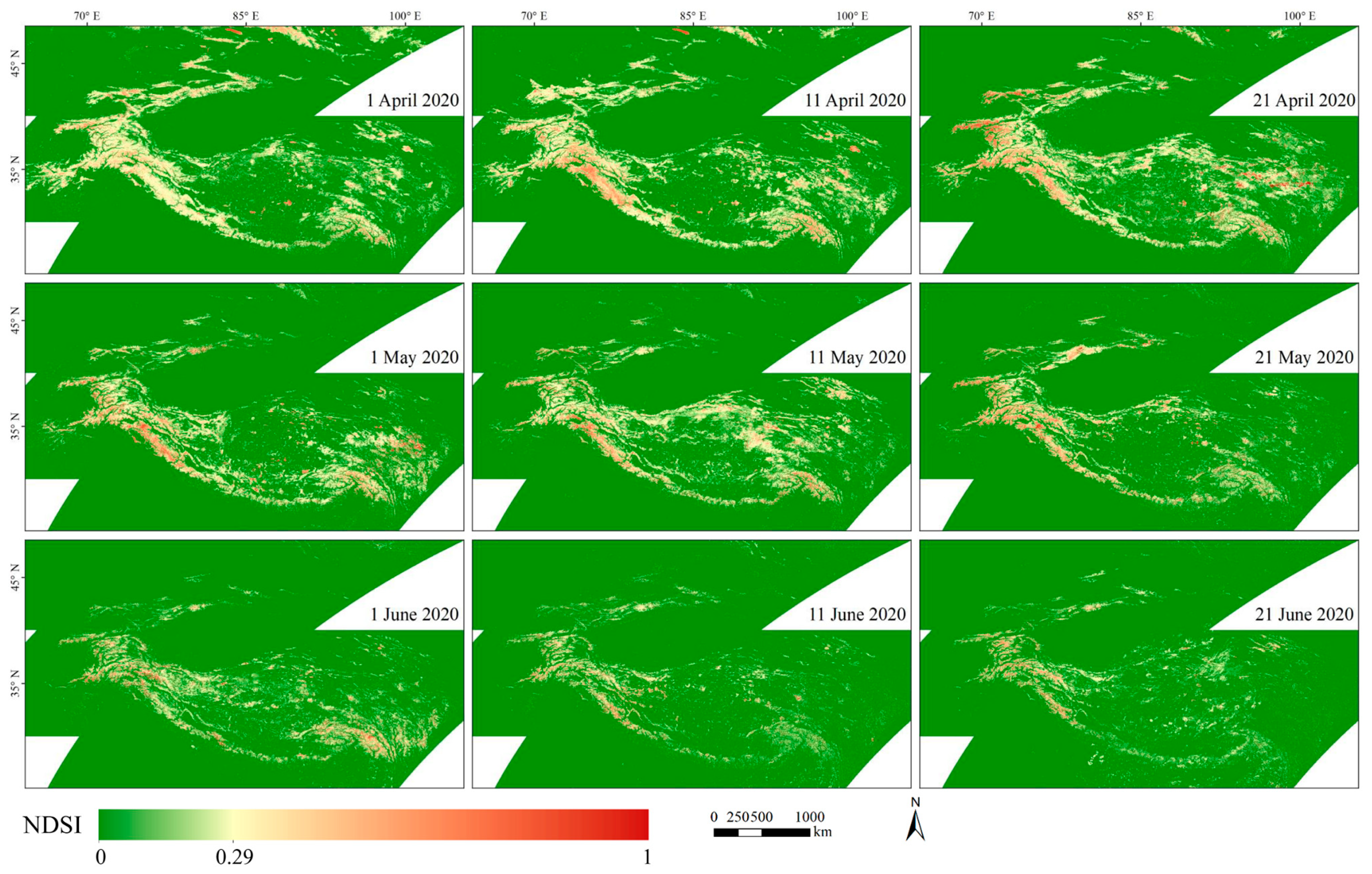
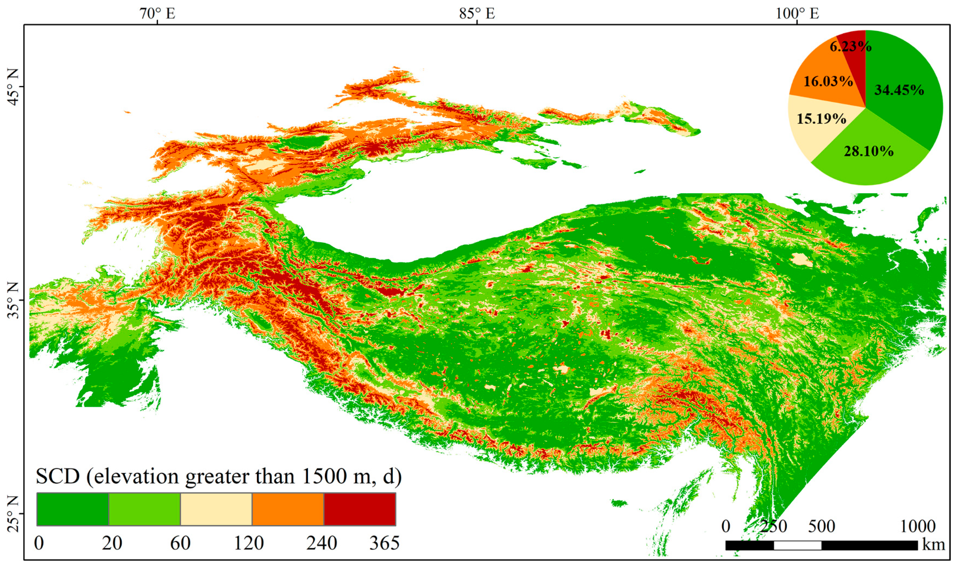
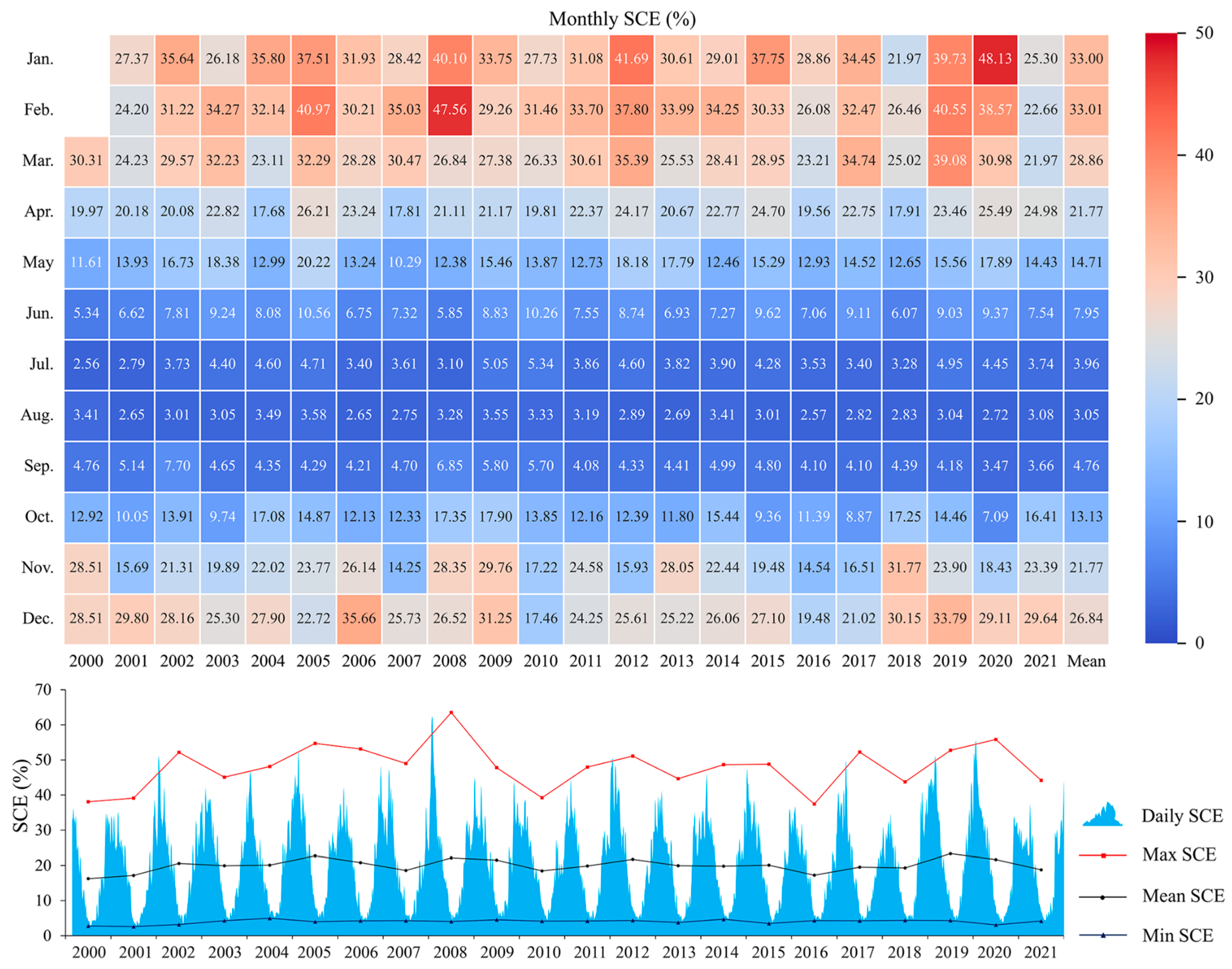
4.3. Spatio-Temporal Patterns of Snow Cover over HMA

The CGF MODIS NDSI product developed in this study can be utilized to detect the spatio-temporal patterns of snow cover over HMA. The snow cover over HMA exhibit large spatial heterogeneity due to the complex topographic and climatic conditions, and a characteristic of a marked reduction in space during the snow melt period (Figure 6). Using 0.29 of the MODIS NDSI threshold, the snow-covered days (SCD) and snow-covered extent (SCE) can be calculated [71]. As seen in Figure 7, the areas with high SCD (SCD > 120 d) are mainly distributed in high-altitude mountain ranges, such as Tien Shan, Karakoram, Kunlun, Qilian Shan, Hengduan Shan and Himalayas, accounting for 22.25% of HMA (elevation greater than 1500 m). The areas with low SCD (SCD < 20 d) are primarily distributed in the interior of the Tibetan Plateau and low altitude areas around it, accounting for 34.45%. Figure 8 displays the interannual variations in the daily snow-covered extent (SCE), monthly SCE and yearly SCE for HMA (elevation greater than 1500 m) from 2000 to 2021. The daily SCE and monthly SCE presents strong interannual volatility in winter months, while there is steady fluctuation in summer months. As for the yearly SCE, the mean SCE and minimum SCE show smooth interannual fluctuations with an insignificant trend. However, the maximum SCE shows significant interannual fluctuation, which can reflect some extreme weather events to some degree, such as the extreme snow event in 2008.

5. Discussion

In recent years, several researchers have successively developed good long-term cloud-free snow cover products for different regional scales (Table 6). Overall, cloud-free SCE products produced by composite algorithms are frequently released, while only a few NDSI products have been produced. The global cloud-gap-filled MODIS NDSI dataset (MOD10A1F) were generated by retaining clear-sky views of the surface from previous days in MOD10A1 NDSI product to fill the cloud-covered pixel [81,82]. However, this product performs poorly in China, where periodic and transient snow is dominant [59], and so does HMA. Jing et al. [59] developed the Spatio-Temporal Adaptive fusion method with erroR correction to generate the cloud-free STAR NDSI collection. This product provides a detailed snow cover dataset with high accuracy for China and have excellent application prospects. Tang et al. [71] developed a cloud removal method based on CSI for MODIS NDSI products. Even though this method effectively filled in the missing data under the cloud cover, it may cause some error in the case of long cloud persistence days. Our study is an inheritance and a great improvement of our previous work [71] in a sense. In this study, three temporal interpolation methods (LI, QI and CSI) and a STW method are synthesized and compared for determining the final CGF method. Accuracy evaluations based on in situ SD observations and high-resolution Landsat-8 OLI images derived snow cover maps verified the reliability of the CGF MODIS NDSI product in terms of accuracy and consistency. In addition, the CGF MODIS NDSI product effectively improves the accuracy of NDSI reconstructions in areas with long cloud persistence days. Additionally based on this high accuracy product, the binary snow cover (BSC) product could be derived using a certain MODIS NDSI threshold (such as 0.29 of Zhang et al. [58]) or the fractional snow cover (FSC) product could be derived using the empirical relationship of Zhang et al. [59] between FSC and MODIS NDSI, which in turn can be engaged in other applications.
However, limitations of the CGF MODIS NDSI product (including its accuracy validation) may come from the following: (1) the original MODIS NDSI products are not perfect due to the difficulty of detecting snow in the mountainous area with complex terrain and land cover, as well as snow/cloud confusion errors in the cloud-masking algorithm for MODIS snow data; (2) the slope and aspect of the terrain, and forest canopy obstruction may affect the reconstruction of NDSI or the accuracy of NDSI from MODIS original products [33,34]; (3) the NDSI approach cannot always accurately distinguish between snow and cloud, which leads to snow misclassification errors [91,92]; (4) the in situ SD observations are sorely scarce, especially in high-altitude areas, which creates challenges in verifying snow category classification [58]; when there is high cloud coverage in Landsat images, aggregating from the Landsat snow cover map with 30 m spatial resolution to the snow cover map with 500 m MODIS spatial resolution may introduce some uncertainties; and (5) there are also spatial inconsistencies between the CGF MODIS NDSI product and Landsat snow cover, possible reasons are as follows: firstly there is a difference between the Landsat OLI and MODIS sensors and their snow cover mapping algorithms; secondly the snow cover information obtained from the two images is inconsistent, even on the same day, because the snow can change rapidly affected by wind speed, sunshine duration, air temperature and precipitation [78]; lastly due to scaling effects, Landsat is superior to MODIS in portraying snow cover in areas of complex terrain. In addition, as the temporal and spatial resolution of satellite remote sensing increases, different strategies need to be adopted when reconstructing snow cover information, taking into account different snow conditions, microtopographic factors (e.g., as slope gradient and aspect), land-cover types and vegetation coverage in forests.

6. Conclusions

The MODIS NDSI snow cover product is susceptible to the influence of the cloud contamination, leading to numerous data gaps. In this study, an effective CGF method was developed to fully fill the data gaps in MODIS NDSI snow cover product. The CGF MODIS NDSI product generally has the following strengths:
(1) The proposed CGF method combines the respective strengths of the CSI method (high accuracy and computational efficiency in the case of short cloud persistence days) and the STW method (comprehensively considering spatial and temporal correlations of the snow cover).
(2) An accuracy evaluation based on in situ SD observations verified the reliability of the CGF MODIS NDSI product in terms of accuracy and consistency. The CGF MODIS NDSI product achieves a high-range OA of 93.54–98.08%, a low-range MU error of 0.15–3.49% and an acceptable-range MO error of 0.84–5.77% for different combinations of NDSI and SD observed thresholds. Compared with the high-resolution Landsat-8 OLI images derived snow cover maps, the CGF MODIS NDSI product largely corresponds to the Landsat snow cover maps, even if there are scaling effects. In addition, the CGF MODIS NDSI product effectively improves the accuracy of NDSI reconstructions in areas with long cloud persistence days.
(3) Overall, the CGF MODIS NDSI product performs well and is able to provide a set of long-term, spatiotemporally continuous and highly accurate snow cover dataset for HMA, and thereby provide a valuable input dataset for hydrological and climate modeling, snow cover dynamics and other water-related studies.

Author Contributions

Conceptualization, Z.T. and G.D.; methodology, Z.T. and G.D.; validation, G.D.; writing—original draft preparation, G.D.; writing—review and editing, Z.T., G.D., C.D., D.S. and X.W.; supervision, Z.T.; funding acquisition, Z.T. and C.D. All authors have read and agreed to the published version of the manuscript.

Funding

This research was supported by the Science and Technology Innovation Program of Hunan Province, China (Grant No. 2022RC1240), the National Natural Science Foundation of China (Grant Nos. 41871058, 41801254), the Scientific Research Foundation of Hunan Education Department, China (Grant No. 23A0363) and the Natural Science Foundation of Hunan Province, China (Grant No. 2022JJ30245).

Data Availability Statement

The daily cloud-gap-filled (CGF) Terra-Aqua MODIS NDSI product and the cloud persistence days (CPD) dataset for High Mountain Asia (HMA) from 2000 to 2021 generated in this study, are available at https://doi.org/10.5281/zenodo.7341828, accessed on 26 November 2022.

Acknowledgments

We would like to thank the National Tibetan Plateau Data Center (http://data.tpdc.ac.cn, accessed on 5 August 2022) for providing the in situ snow depth observations over the Tibetan Plateau. We would like to thank the editors and anonymous reviewers for their helpful comments and constructive suggestions.

Conflicts of Interest

The authors declare no conflict of interest.

Appendix A

Table A1. Summary table of abbreviations of key terminology in this paper.
No.AbbreviationFull Terminology
1BSCBinary snow cover
2CGFCloud-gap-filled
3CPDCloud persistence days
4CECommission error
5CSICubic spline interpolation
6HMAHigh Mountain Asia
7LILinear interpolation
8MAEMean absolute error
9MODISModerate Resolution Imaging Spectroradiometer
10NDSINormalized difference snow index
11OEOmission error
12OAOverall accuracy
13MOOverestimation error
14QIQuadratic interpolation
15RMSERoot–mean–square–error
16SCDSnow-covered days
17SCESnow-covered extent
18SDSnow depth
19STWSpatio-temporal weighted
20TACTerra and Aqua combination
21TITemporal interpolation
22MUUnderestimation error
Table A2. Statistical description of Landsat-8 OLI images used for comparison and validation of the CGF MODIS NDSI product in this study.
Image Pair No.Path/RowDate of AcquisitionCloud Cover (%)
1134/372017/04/184.28
2134/402017/06/0511.78
3134/402020/02/064.82
4134/402021/03/284.44
5135/332017/11/192.72
6135/332019/05/013.12
7135/332021/12/162.61
8140/362018/04/1511.66
9141/362021/11/082.92
10141/402016/12/282.78
11141/402018/05/0813.14
12141/402019/02/043.49
13141/402021/12/102.95
14142/372016/01/187.05
15142/372021/12/173.23
16143/362017/06/0412.29
17143/362021/11/220.29
18144/362021/11/132.04
19145/302016/03/2726.43
20145/302018/10/274.9
21145/302019/09/126.61
22145/392017/06/0212.39
23145/392018/04/186.15
24145/392019/12/013.27
25145/392020/02/032.31
26145/392021/04/262.75
27146/352016/07/243.83
28146/352018/05/113.37
29147/372017/01/233.26
30147/372017/07/0213.45
31147/372018/06/032.45
32147/372019/10/281.49
33148/352016/12/2928.13
34148/352018/05/0912.37
35148/352019/06/2913.19
36149/342018/01/242.99
37149/342021/07/112.26
38150/342016/07/202.46
39150/342016/11/094.46
40151/332017/04/090.3
41151/332019/05/014.46
42151/332020/08/232.37
43151/332021/07/091.59
44151/352017/04/090.43
45151/352019/05/019.88

References

  1. Dietz, A.J.; Kuenzer, C.; Gessner, U.; Dech, S. Remote sensing of snow—A review of available methods. Int. J. Remote Sens. 2012, 33, 4094–4134. [Google Scholar] [CrossRef]
  2. Hall, D.K.; Riggs, G.A.; Salomonson, V.V. Development of methods for mapping global snow cover using moderate resolution imaging spectroradiometer data. Remote Sens. Environ. 1995, 54, 127–140. [Google Scholar] [CrossRef]
  3. Hori, M.; Sugiura, K.; Kobayashi, K.; Aoki, T.; Tanikawa, T.; Kuchiki, K.; Niwano, M.; Enomoto, H. A 38-year (1978–2015) Northern Hemisphere daily snow cover extent product derived using consistent objective criteria from satellite-borne optical sensors. Remote Sens. Environ. 2017, 191, 402–418. [Google Scholar] [CrossRef]
  4. Dong, C. Remote sensing, hydrological modeling and in situ observations in snow cover research: A review. J. Hydrol. 2018, 561, 573–583. [Google Scholar] [CrossRef]
  5. Groisman, P.Y.; Karl, T.R.; Knight, R.W. Observed impact of snow cover on the heat balance and the rise of continental spring temperatures. Science 1994, 263, 198–200. [Google Scholar] [CrossRef] [PubMed]
  6. Kang, S.; Xu, Y.; You, Q.; Flügel, W.-A.; Pepin, N.; Yao, T. Review of climate and cryospheric change in the Tibetan Plateau. Environ. Res. Lett. 2010, 5, 015101. [Google Scholar] [CrossRef]
  7. You, Q.; Wu, T.; Shen, L.; Pepin, N.; Zhang, L.; Jiang, Z.; Wu, Z.; Kang, S.; AghaKouchak, A. Review of snow cover variation over the Tibetan Plateau and its influence on the broad climate system. Earth Sci. Rev. 2020, 201, 103043. [Google Scholar] [CrossRef]
  8. Barnett, T.P.; Adam, J.C.; Lettenmaier, D.P. Potential impacts of a warming climate on water availability in snow-dominated regions. Nature 2005, 438, 303–309. [Google Scholar] [CrossRef]
  9. Bormann, K.J.; Brown, R.D.; Derksen, C.; Painter, T.H. Estimating snow-cover trends from space. Nat. Clim. Chang. 2018, 8, 924–928. [Google Scholar] [CrossRef]
  10. Li, H.; Li, X.; Yang, D.; Wang, J.; Gao, B.; Pan, X.; Zhang, Y.; Hao, X. Tracing snowmelt paths in an integrated hydrological model for understanding seasonal snowmelt contribution at basin scale. J. Geophys. Res. Atmos. 2019, 124, 8874–8895. [Google Scholar] [CrossRef]
  11. Immerzeel, W.W.; Lutz, A.; Andrade, M.; Bahl, A.; Biemans, H.; Bolch, T.; Hyde, S.; Brumby, S.; Davies, B.; Elmore, A. Importance and vulnerability of the world’s water towers. Nature 2020, 577, 364–369. [Google Scholar] [CrossRef] [PubMed]
  12. Immerzeel, W.W.; Van Beek, L.P.; Bierkens, M.F. Climate change will affect the Asian water towers. Science 2010, 328, 1382–1385. [Google Scholar] [CrossRef] [PubMed]
  13. Yao, T. Tackling on environmental changes in Tibetan Plateau with focus on water, ecosystem and adaptation. Sci. Bull. 2019, 64, 417. [Google Scholar] [CrossRef] [PubMed]
  14. Baghdadi, N.; Gauthier, Y.; Bernier, M. Capability of multitemporal ERS-1 SAR data for wet-snow mapping. Remote Sens. Environ. 1997, 60, 174–186. [Google Scholar] [CrossRef]
  15. Che, T.; Dai, L.; Zheng, X.; Li, X.; Zhao, K. Estimation of snow depth from passive microwave brightness temperature data in forest regions of northeast China. Remote Sens. Environ. 2016, 183, 334–349. [Google Scholar] [CrossRef]
  16. Liang, T.; Zhang, X.; Xie, H.; Wu, C.; Feng, Q.; Huang, X.; Chen, Q. Toward improved daily snow cover mapping with advanced combination of MODIS and AMSR-E measurements. Remote Sens. Environ. 2008, 112, 3750–3761. [Google Scholar] [CrossRef]
  17. Romanov, P.; Gutman, G.; Csiszar, I. Automated monitoring of snow cover over North America with multispectral satellite data. J. Appl. Meteorol. 2000, 39, 1866–1880. [Google Scholar] [CrossRef]
  18. Li, X.; Jing, Y.; Shen, H.; Zhang, L. The recent developments in cloud removal approaches of MODIS snow cover product. Hydrol. Earth Syst. Sci. 2019, 23, 2401–2416. [Google Scholar] [CrossRef]
  19. Lievens, H.; Demuzere, M.; Marshall, H.-P.; Reichle, R.H.; Brucker, L.; Brangers, I.; de Rosnay, P.; Dumont, M.; Girotto, M.; Immerzeel, W.W. Snow depth variability in the Northern Hemisphere mountains observed from space. Nat. Commun. 2019, 10, 4629. [Google Scholar] [CrossRef]
  20. Smith, T.; Bookhagen, B. Changes in seasonal snow water equivalent distribution in High Mountain Asia (1987 to 2009). Sci. Adv. 2018, 4, e1701550. [Google Scholar] [CrossRef]
  21. Tedesco, M.; Narvekar, P.S. Assessment of the nasa amsr-e swe product. IEEE J. Sel. Top. Appl. Earth Obs. Remote Sens. 2010, 3, 141–159. [Google Scholar] [CrossRef]
  22. Crawford, C.J.; Manson, S.M.; Bauer, M.E.; Hall, D.K. Multitemporal snow cover mapping in mountainous terrain for Landsat climate data record development. Remote Sens. Environ. 2013, 135, 224–233. [Google Scholar] [CrossRef]
  23. Hüsler, F.; Jonas, T.; Riffler, M.; Musial, J.P.; Wunderle, S. A satellite-based snow cover climatology (1985–2011) for the European Alps derived from AVHRR data. Cryosphere 2014, 8, 73–90. [Google Scholar] [CrossRef]
  24. Jing, Y.; Shen, H.; Li, X.; Guan, X. A two-stage fusion framework to generate a spatio–temporally continuous MODIS NDSI product over the Tibetan Plateau. Remote Sens. 2019, 11, 2261. [Google Scholar] [CrossRef]
  25. Simic, A.; Fernandes, R.; Brown, R.; Romanov, P.; Park, W. Validation of VEGETATION, MODIS, and GOES+ SSM/I snow-cover products over Canada based on surface snow depth observations. Hydrol. Process. 2004, 18, 1089–1104. [Google Scholar] [CrossRef]
  26. Naegeli, K.; Neuhaus, C.; Salberg, A.; Schwaizer, G.; Wiesmann, A.; Wunderle, S.; Nagler, T. ESA Snow Climate Change Initiative (Snow_cci): Daily Global Snow Cover Fraction—Snow on Ground (SCFG) from AVHRR (1982–2019), version 1.0.; Centre for Environmental Data Analysis: Chilton, UK, 2021. [Google Scholar] [CrossRef]
  27. Riggs, G.A.; Hall, D.K. NASA S-NPP VIIRS Snow Cover Products Collection 2 User Guide; National Snow and Ice Data Center: Boulder, CO, USA, 2021. Available online: https://modis-snow-ice.gsfc.nasa.gov/uploads/VIIRS_snow_products_user_guide_version_2.pdf (accessed on 2 August 2022).
  28. Riggs, G.A.; Hall, D.K.; Román, M.O. MODIS Snow Products Collection 6 User Guide; National Snow and Ice Data Center: Boulder, CO, USA, 2015. Available online: https://modis-snow-ice.gsfc.nasa.gov/uploads/snow_user_guide_C6.1_final_revised_april.pdf (accessed on 10 April 2022).
  29. Huang, X.; Liang, T.; Zhang, X.; Guo, Z. Validation of MODIS snow cover products using Landsat and ground measurements during the 2001–2005 snow seasons over northern Xinjiang, China. Int. J. Remote Sens. 2011, 32, 133–152. [Google Scholar] [CrossRef]
  30. Parajka, J.; Blöschl, G. Validation of MODIS snow cover images over Austria. Hydrol. Earth Syst. Sci. 2006, 10, 679–689. [Google Scholar] [CrossRef]
  31. Tang, Z.; Wang, J.; Li, H.; Yan, L. Spatiotemporal changes of snow cover over the Tibetan plateau based on cloud-removed moderate resolution imaging spectroradiometer fractional snow cover product from 2001 to 2011. J. Appl. Remote Sens. 2013, 7, 073582. [Google Scholar] [CrossRef]
  32. Yang, J.; Jiang, L.; Ménard, C.B.; Luojus, K.; Lemmetyinen, J.; Pulliainen, J. Evaluation of snow products over the Tibetan Plateau. Hydrol. Process. 2015, 29, 3247–3260. [Google Scholar] [CrossRef]
  33. Xiao, X.; He, T.; Liang, S.; Liu, X.; Ma, Y.; Liang, S.; Chen, X. Estimating fractional snow cover in vegetated environments using MODIS surface reflectance data. Int. J. Appl. Earth Obs. Geoinf. 2022, 114, 103030. [Google Scholar] [CrossRef]
  34. Luo, J.; Dong, C.; Lin, K.; Chen, X.; Zhao, L.; Menzel, L. Mapping snow cover in forests using optical remote sensing, machine learning and time-lapse photography. Remote Sens. Environ. 2022, 275, 113017. [Google Scholar] [CrossRef]
  35. Deng, G.; Tang, Z.; Hu, G.; Wang, J.; Sang, G.; Li, J. Spatiotemporal dynamics of snowline altitude and their responses to climate change in the Tienshan Mountains, Central Asia, During 2001–2019. Sustainability 2021, 13, 3992. [Google Scholar] [CrossRef]
  36. Hall, D.K.; Riggs, G.A. Accuracy assessment of the MODIS snow products. Hydrol. Process. 2007, 21, 1534–1547. [Google Scholar] [CrossRef]
  37. Hall, D.K.; Riggs, G.A.; Salomonson, V.V.; DiGirolamo, N.E.; Bayr, K.J. MODIS snow-cover products. Remote Sens. Environ. 2002, 83, 181–194. [Google Scholar] [CrossRef]
  38. Parajka, J.; Blöschl, G. Spatio-temporal combination of MODIS images–potential for snow cover mapping. Water Resour. Res. 2008, 44, W03406. [Google Scholar] [CrossRef]
  39. Lindsay, C.; Zhu, J.; Miller, A.E.; Kirchner, P.; Wilson, T.L. Deriving snow cover metrics for Alaska from MODIS. Remote Sens. 2015, 7, 12961–12985. [Google Scholar] [CrossRef]
  40. Paudel, K.P.; Andersen, P. Monitoring snow cover variability in an agropastoral area in the Trans Himalayan region of Nepal using MODIS data with improved cloud removal methodology. Remote Sens. Environ. 2011, 115, 1234–1246. [Google Scholar] [CrossRef]
  41. Dietz, A.J.; Wohner, C.; Kuenzer, C. European snow cover characteristics between 2000 and 2011 derived from improved MODIS daily snow cover products. Remote Sens. 2012, 4, 2432–2454. [Google Scholar] [CrossRef]
  42. Gafurov, A.; Bárdossy, A. Cloud removal methodology from MODIS snow cover product. Hydrol. Earth Syst. Sci. 2009, 13, 1361–1373. [Google Scholar] [CrossRef]
  43. Dozier, J.; Painter, T.H.; Rittger, K.; Frew, J.E. Time–space continuity of daily maps of fractional snow cover and albedo from MODIS. Adv. Water Resour. 2008, 31, 1515–1526. [Google Scholar] [CrossRef]
  44. Tang, Z.; Wang, J.; Li, H.; Liang, J.; Li, C.; Wang, X. Extraction and assessment of snowline altitude over the Tibetan plateau using MODIS fractional snow cover data (2001 to 2013). J. Appl. Remote Sens. 2014, 8, 084689. [Google Scholar] [CrossRef]
  45. Tang, Z.; Wang, X.; Wang, J.; Wang, X.; Li, H.; Jiang, Z. Spatiotemporal variation of snow cover in Tianshan Mountains, Central Asia, based on cloud-free MODIS fractional snow cover product, 2001–2015. Remote Sens. 2017, 9, 1045. [Google Scholar] [CrossRef]
  46. Parajka, J.; Pepe, M.; Rampini, A.; Rossi, S.; Blöschl, G. A regional snow-line method for estimating snow cover from MODIS during cloud cover. J. Hydrol. 2010, 381, 203–212. [Google Scholar] [CrossRef]
  47. López-Burgos, V.; Gupta, H.; Clark, M. Reducing cloud obscuration of MODIS snow cover area products by combining spatio-temporal techniques with a probability of snow approach. Hydrol. Earth Syst. Sci. 2013, 17, 1809–1823. [Google Scholar] [CrossRef]
  48. Brown, R.; Derksen, C.; Wang, L. A multi-data set analysis of variability and change in Arctic spring snow cover extent, 1967–2008. J. Geophys. Res. Atmos. 2010, 115, D16111. [Google Scholar] [CrossRef]
  49. Gafurov, A.; Vorogushyn, S.; Farinotti, D.; Duethmann, D.; Merkushkin, A.; Merz, B. Snow-cover reconstruction methodology for mountainous regions based on historic in situ observations and recent remote sensing data. Cryosphere 2015, 9, 451–463. [Google Scholar] [CrossRef]
  50. Huang, X.; Deng, J.; Ma, X.; Wang, Y.; Feng, Q.; Hao, X.; Liang, T. Spatiotemporal dynamics of snow cover based on multi-source remote sensing data in China. Cryosphere 2016, 10, 2453–2463. [Google Scholar] [CrossRef]
  51. Poggio, L.; Gimona, A. Sequence-based mapping approach to spatio-temporal snow patterns from MODIS time-series applied to Scotland. Int. J. Appl. Earth Obs. Geoinf. 2015, 34, 122–135. [Google Scholar] [CrossRef]
  52. Hou, J.; Huang, C.; Zhang, Y.; Guo, J.; Gu, J. Gap-filling of modis fractional snow cover products via non-local spatio-temporal filtering based on machine learning techniques. Remote Sens. 2019, 11, 90. [Google Scholar] [CrossRef]
  53. Huang, Y.; Liu, H.; Yu, B.; Wu, J.; Kang, E.L.; Xu, M.; Wang, S.; Klein, A.; Chen, Y. Improving MODIS snow products with a HMRF-based spatio-temporal modeling technique in the Upper Rio Grande Basin. Remote Sens. Environ. 2018, 204, 568–582. [Google Scholar] [CrossRef]
  54. Li, X.; Fu, W.; Shen, H.; Huang, C.; Zhang, L. Monitoring snow cover variability (2000–2014) in the Hengduan Mountains based on cloud-removed MODIS products with an adaptive spatio-temporal weighted method. J. Hydrol. 2017, 551, 314–327. [Google Scholar] [CrossRef]
  55. Xia, Q.; Gao, X.; Chu, W.; Sorooshian, S. Estimation of daily cloud-free, snow-covered areas from MODIS based on variational interpolation. Water Resour. Res. 2012, 48, W09523. [Google Scholar] [CrossRef]
  56. Riggs, G.A.; Hall, D.K.; Román, M.O. Overview of NASA’s MODIS and visible infrared imaging radiometer suite (VIIRS) snow-cover earth system data records. Earth Syst. Sci. Data 2017, 9, 765–777. [Google Scholar] [CrossRef]
  57. Zhang, H.; Zhang, F.; Zhang, G.; Che, T.; Yan, W.; Ye, M.; Ma, N. Ground-based evaluation of MODIS snow cover product V6 across China: Implications for the selection of NDSI threshold. Sci. Total Environ. 2019, 651, 2712–2726. [Google Scholar] [CrossRef] [PubMed]
  58. Zhang, H.; Zhang, F.; Zhang, G.; Yan, W.; Li, S. Enhanced scaling effects significantly lower the ability of MODIS normalized difference snow index to estimate fractional and binary snow cover on the Tibetan Plateau. J. Hydrol. 2021, 592, 125795. [Google Scholar] [CrossRef]
  59. Jing, Y.; Li, X.; Shen, H. STAR NDSI collection: A cloud-free MODIS NDSI dataset (2001–2020) for China. Earth Syst. Sci. Data 2022, 14, 3137–3156. [Google Scholar] [CrossRef]
  60. Arendt, A.; Bliss, A.; Bolch, T.; Cogley, J.; Gardner, A.; Hagen, J.-O.; Hock, R.; Huss, M.; Kaser, G.; Kienholz, C. Randolph Glacier Inventory—A Dataset of Global Glacier Outlines: Version 6.0: Technical Report, Global Land Ice Measurements from Space; National Snow and Ice Data Center: Boulder, CO, USA, 2017. [Google Scholar] [CrossRef]
  61. Khanal, S.; Lutz, A.F.; Kraaijenbrink, P.D.; van den Hurk, B.; Yao, T.; Immerzeel, W.W. Variable 21st century climate change response for rivers in High Mountain Asia at seasonal to decadal time scales. Water Resour. Res. 2021, 57, e2020WR029266. [Google Scholar] [CrossRef]
  62. Liu, Y.; Fang, Y.; Margulis, S.A. Spatiotemporal distribution of seasonal snow water equivalent in High Mountain Asia from an 18-year Landsat–MODIS era snow reanalysis dataset. Cryosphere 2021, 15, 5261–5280. [Google Scholar] [CrossRef]
  63. Tang, Z.; Wang, X.; Deng, G.; Wang, X.; Jiang, Z.; Sang, G. Spatiotemporal variation of snowline altitude at the end of melting season across High Mountain Asia, using MODIS snow cover product. Adv. Space Res. 2020, 66, 2629–2645. [Google Scholar] [CrossRef]
  64. Wei, J.; Liu, S.; Guo, W.; Yao, X.; Xu, J.; Bao, W.; Jiang, Z. Surface-area changes of glaciers in the Tibetan Plateau interior area since the 1970s using recent Landsat images and historical maps. Ann. Glaciol. 2014, 55, 213–222. [Google Scholar] [CrossRef]
  65. Yao, T.; Bolch, T.; Chen, D.; Gao, J.; Immerzeel, W.; Piao, S.; Su, F.; Thompson, L.; Wada, Y.; Wang, L. The imbalance of the Asian water tower. Nat. Rev. Earth Environ. 2022, 3, 618–632. [Google Scholar] [CrossRef]
  66. Liu, Y.; Li, Z.; Chen, Y. Continuous warming shift greening towards browning in the Southeast and Northwest High Mountain Asia. Sci. Rep. 2021, 11, 17920. [Google Scholar] [CrossRef] [PubMed]
  67. Chen, X.; Liang, S.; Cao, Y.; He, T.; Wang, D. Observed contrast changes in snow cover phenology in northern middle and high latitudes from 2001–2014. Sci. Rep. 2015, 5, 16820. [Google Scholar] [CrossRef] [PubMed]
  68. Wang, K.; Zhang, L.; Qiu, Y.; Ji, L.; Tian, F.; Wang, C.; Wang, Z. Snow effects on alpine vegetation in the Qinghai-Tibetan Plateau. Int. J. Digital Earth 2015, 8, 58–75. [Google Scholar] [CrossRef]
  69. Chu, D.; Luosang, Q.; Lin, Z.; Yang, Y. Spatial-temporal variation of snow depth on Tibetan Plateau over the last 30 years. Meteor. Mon. 2018, 44, 233–243. [Google Scholar] [CrossRef]
  70. National Meteorological Information Center; Tibet Meteorological Bureau, China. Observational Snow Depth Dataset of the Tibetan Plateau (Version 1.0) (1961–2013); National Tibetan Plateau Data Center: Beijing, China, 2018. [Google Scholar] [CrossRef]
  71. Tang, Z.; Deng, G.; Hu, G.; Zhang, H.; Pan, H.; Sang, G. Satellite observed spatiotemporal variability of snow cover and snow phenology over High Mountain Asia from 2002 to 2021. J. Hydrol. 2022, 613, 128438. [Google Scholar] [CrossRef]
  72. Chen, S.; Wang, X.; Guo, H.; Xie, P.; Wang, J.; Hao, X. A conditional probability interpolation method based on a space-time cube for modis snow cover products gap filling. Remote Sens. 2020, 12, 3577. [Google Scholar] [CrossRef]
  73. Jin, X.; Ke, C.Q.; Xu, Y.Y.; Li, X.C. Spatial and temporal variations of snow cover in the Loess Plateau, China. Int. J. Climatol. 2015, 35, 1721–1731. [Google Scholar] [CrossRef]
  74. Sharma, V.; Mishra, V.; Joshi, P. Topographic controls on spatio-temporal snow cover distribution in Northwest Himalaya. Int. J. Remote Sens. 2014, 35, 3036–3056. [Google Scholar] [CrossRef]
  75. Tong, J.; Déry, S.; Jackson, P. Topographic control of snow distribution in an alpine watershed of western Canada inferred from spatially-filtered MODIS snow products. Hydrol. Earth Syst. Sci. 2009, 13, 319–326. [Google Scholar] [CrossRef]
  76. Hou, J.; Huang, C.; Zhang, Y.; You, Y. Reconstructing a Gap-Free MODIS Normalized Difference Snow Index Product Using a Long Short-Term Memory Network. IEEE Trans. Geosci. Remote Sens. 2022, 60, 1–14. [Google Scholar] [CrossRef]
  77. Klein, A.G.; Hall, D.K.; Riggs, G.A. Improving snow cover mapping in forests through the use of a canopy reflectance model. Hydrol. Process. 1998, 12, 1723–1744. [Google Scholar] [CrossRef]
  78. Liu, C.; Li, Z.; Zhang, P.; Zeng, J.; Gao, S.; Zheng, Z. An Assessment and Error Analysis of MOD10A1 Snow Product Using Landsat and Ground Observations Over China During 2000–2016. IEEE J. Sel. Top. Appl. Earth Obs. Remote Sens. 2020, 13, 1467–1478. [Google Scholar] [CrossRef]
  79. Wang, X.; Wang, J.; Jiang, Z.; Li, H.; Hao, X. An effective method for snow-cover mapping of dense coniferous forests in the Upper Heihe River Basin using Landsat Operational Land Imager data. Remote Sens. 2015, 7, 17246–17257. [Google Scholar] [CrossRef]
  80. Wang, X.; Wang, J.; Che, T.; Huang, X.; Hao, X.; Li, H. Snow cover mapping for complex mountainous forested environments based on a multi-index technique. IEEE J. Sel. Top. Appl. Earth Obs. Remote Sens. 2018, 11, 1433–1441. [Google Scholar] [CrossRef]
  81. Hall, D.K.; Riggs, G.A. MODIS/Terra CGF Snow Cover Daily L3 Global 500 m SIN Grid, version 61; National Snow and Ice Data Center: Boulder, CO, USA, 2020. [Google Scholar] [CrossRef]
  82. Hall, D.K.; Riggs, G.A.; Foster, J.L.; Kumar, S.V. Development and evaluation of a cloud-gap-filled MODIS daily snow-cover product. Remote Sens. Environ. 2010, 114, 496–503. [Google Scholar] [CrossRef]
  83. Huang, X. MODIS Daily Cloudless Binary Snow Products in Northern Hemisphere from 2000 to 2015; National Cryosphere Desert Data Center: Lanzhou, China, 2020. [Google Scholar] [CrossRef]
  84. Hao, X.; Huang, G.; Che, T.; Ji, W.; Sun, X.; Zhao, Q.; Zhao, H.; Wang, J.; Li, H.; Yang, Q. The NIEER AVHRR snow cover extent product over China–a long-term daily snow record for regional climate research. Earth Syst. Sci. Data 2021, 13, 4711–4726. [Google Scholar] [CrossRef]
  85. Hao, X.; Huang, G.; Zheng, Z.; Sun, X.; Ji, W.; Zhao, H.; Wang, J.; Li, H.; Wang, X. Development and validation of a new MODIS snow-cover-extent product over China. Hydrol. Earth Syst. Sci. 2022, 26, 1937–1952. [Google Scholar] [CrossRef]
  86. Muhammad, S.; Thapa, A. An improved Terra–Aqua MODIS snow cover and Randolph Glacier Inventory 6.0 combined product (MOYDGL06*) for high-mountain Asia between 2002 and 2018. Earth Syst. Sci. Data 2020, 12, 345–356. [Google Scholar] [CrossRef]
  87. Huang, Y.; Xu, J.; Xu, J.; Zhao, Y.; Yu, B.; Liu, H.; Wang, S.; Xu, W.; Wu, J.; Zheng, Z. HMRFS–TP: Long-term daily gap-free snow cover products over the Tibetan Plateau from 2002 to 2021 based on hidden Markov random field model. Earth Syst. Sci. Data 2022, 14, 4445–4462. [Google Scholar] [CrossRef]
  88. Li, Y.; Sun, F.; Chen, Y.; Li, B.; Fang, G.; Duan, W.; Xia, Q. The continuing shrinkage of snow cover in High Mountain Asia over the last four decades. Sci. Bull. 2022, 67, 2064–2068. [Google Scholar] [CrossRef] [PubMed]
  89. Qiu, Y.; Wang, X.; Han, L.; Chang, L.; Shi, L. Daily Fractional Snow Cover (FSC) Data Set over High Asia; Science Data Bank: Beijing, China, 2017. [Google Scholar] [CrossRef]
  90. Han, C.; Shen, Y.; Ouyang, Z.; Xie, P.; Guo, H.; Chen, S.; Wang, X. Daily Cloudless NDSI Data Set with 500m Resolution Snow Season in Northeast China (2000–2020); National Cryosphere Desert Data Center: Lanzhou, China, 2021. [Google Scholar] [CrossRef]
  91. Dong, C.; Menzel, L. Producing cloud-free MODIS snow cover products with conditional probability interpolation and meteorological data. Remote Sens. Environ. 2016, 186, 439–451. [Google Scholar] [CrossRef]
  92. Wang, G.; Jiang, L.; Shi, J.; Su, X. A universal ratio snow index for fractional snow cover estimation. IEEE Geosci. Remote Sens. Lett. 2020, 18, 721–725. [Google Scholar] [CrossRef]
Figure 1. Topography and location of the HMA. In names of subregions from RGI v6.0, these individual letters ‘W’, ‘C’, ‘E’ and ‘S’ correspond to west, central, east and south, respectively. The location of meteorological stations and Landsat-8 OLI scenes utilized for validation, and the verification regions are also shown.
Remotesensing 16 00192 g001
Figure 2. Schematic of the generation procedure and evaluation of the CGF NDSI product.
Remotesensing 16 00192 g002
Figure 3. (a) The mean frequency of CPD from 2017 to 2021, and (b) MAE and (c) RMSE of retrieved NDSI data using different TI methods and STW method under different CPD conditions. The dashed line indicates that CPD is equal to 8 d.
Remotesensing 16 00192 g003
Figure 4. Comparison of TAC NDSI (column 1), CSI NDSI (column 4), STW NDSI (column 5) and CSI-STW NDSI (column 6) in the three regions (R1, R2 and R3), for 10 November 2020.
Remotesensing 16 00192 g004
Figure 5. Comparison of TAC BSC (row 1), Landsat BSC (row 2), Landsat BSC aggregation (row 3), CSI-STW BSC (row 4) corresponding to four Landsat scenes (column 1–4).
Remotesensing 16 00192 g005
Figure 6. A sequence of the CGF NDSI collection from 1 April 2020 to 21 June 2020.
Remotesensing 16 00192 g006
Figure 7. The spatial distribution of the average SCD for HMA (elevation greater than 1500 m) from 2001 to 2021.
Remotesensing 16 00192 g007
Figure 8. Dynamic variations in monthly SCE (including multi-year mean monthly SCE), daily SCE and yearly SCE (including the maximum SCE, mean SCE and minimum SCE) for HMA (elevation greater than 1500 m) from 2000 to 2021.
Remotesensing 16 00192 g008
Table 1. Accuracy evaluation of confusion matrix based on in situ SD observations. The metrics derived from confusion matrix are: overall accuracy (OA), underestimation error (MU) and overestimation error (MO). The ε1 and ε2 indicate the defined SD threshold value and MODIS NDSI threshold value, respectively.
Observed SD
Snow Cover (≥ε1 cm)No Snow (<ε1 cm)
MODIS NDSISnow cover (≥ε2)ab
No Snow (<ε2)cd
Cloudef
OA = ((a + d)/(a + b + c + d + e + f)) × 100%
MU = (c/(a + b + c + d)) × 100%   MO = (b/(a + b + c + d)) × 100%
Number of available pixels = a + b + c + d
Table 2. Confusion matrix comparing MODIS NDSI derived BSC maps with Landsat BSC maps. The ε2 indicates the defined MODIS NDSI threshold value.
Landsat OLI
Snow CoverNo Snow
MODIS NDSISnow cover (≥ε2) SSNS
No now (<ε2)SNNN
OA = ((SS + NN)/(SS + NS + SN + NN)) × 100%
OE = (SN/(SS + SN)) × 100%   CE = (NS/(NN + NS)) × 100%
Table 3. Validation results for TAC NDSI and CSI-STW NDSI based on in situ SD observations in the Tibetan Plateau from 1 January 2001 to 31 December 2013. The definitions and calculations of the indices in this table are shown in Table 1.
Threshold Values
for Snow Cover
TAC NDSICSI-STW NDSI
OA
(%)
MU
(%)
MO
(%)
OA
(%)
MU
(%)
MO
(%)
ε1 = 1 cm, ε2 = 0.159.211.703.2393.542.324.14
ε1 = 1 cm, ε2 = 0.2960.262.071.1695.393.151.46
ε1 = 1 cm, ε2 = 0.460.432.260.7095.673.490.84
ε1 = 2 cm, ε2 = 0.159.610.713.5794.161.194.65
ε1 = 2 cm, ε2 = 0.2960.860.931.3496.711.561.73
ε1 = 2 cm, ε2 = 0.461.101.070.8397.181.811.01
ε1 = 3 cm, ε2 = 0.159.660.323.8794.300.615.10
ε1 = 3 cm, ε2 = 0.2961.030.451.5597.150.832.02
ε1 = 3 cm, ε2 = 0.461.330.540.9997.780.991.22
ε1 = 5 cm, ε2 = 0.159.520.084.3594.080.155.77
ε1 = 5 cm, ε2 = 0.2961.000.111.9497.260.202.54
ε1 = 5 cm, ε2 = 0.461.360.151.3398.080.271.65
Average value60.450.872.0795.941.392.68
Number of available pixels289,595465,010
Table 4. Validation results for TAC NDSI and CSI-STW NDSI based on Landsat-8 BSC maps under clear-sky conditions. The definitions and calculations of the indices in this table are shown in Table 2.
Metrics
(%)
NDSI Threshold: 0.1NDSI Threshold: 0.29NDSI Threshold: 0.40
TAC NDSICSI-STW NDSITAC NDSICSI-STW NDSITAC NDSICSI-STW NDSI
SS1,765,5242,255,7001,688,2782,158,0141,608,4922,053,084
NS575,201662,668290,431340,524190,413225,094
SN21,23432,57798,480130,263178,266235,193
NN2,990,5393,107,6873,275,3093,429,8313,375,3273,545,261
Total5,352,4986,058,6325,352,4986,058,6325,352,4986,058,632
OE1.191.425.515.699.9810.28
CE16.1317.588.159.035.345.97
OA88.8688.5292.7392.2393.1192.40
Table 5. Validation results of CSI-STW NDSI for filling the data-gap pixels in the TAC NDSI dataset, based on the Landsat-8 BSC maps under clear-sky conditions. The definitions and calculations of the indices in this table are shown in Table 2.
Metrics
(%)
NDSI Threshold: 0.1NDSI Threshold: 0.29NDSI Threshold: 0.40
SS489,451469,736444,592
NS85,16350,09334,681
SN12,06831,78356,927
NN119,452154,522169,934
Total706,134706,134706,134
OE2.416.3411.35
CE41.6224.4816.95
OA86.2388.4187.03
Table 6. Typical long-term cloud-free snow cover products for different regional scales.
Product TypeReferences and Dataset DOISpatial
Coverage
Temporal CoverageTemporal ResolutionSpatial Resolution
SCEHuang [83]
https://doi.org/10.12072/ncdc.CCI.db0044.2020, accessed on 21 March 2022
Northern Hemisphere2000–2015Daily∼1 km
SCEHao et al. [84]
https://doi.org/10.11888/Snow.tpdc.271381, accessed on 21 March 2022
China1981–2019Daily∼5 km
SCEHao et al. [85]
https://doi.org/10.12072/ncdc.I-SNOW.db0001.2020, accessed on 15 May 2022
China2000–2020Daily∼500 m
SCEMuhammad and Thapa [86]
https://doi.org/10.1594/PANGAEA.918198, accessed on 21 March 2022
HMA2002–2019Daily∼500 m
SCEHuang et al. [87]
https://doi.org/10.11888/Cryos.tpdc.272204, accessed on 30 September 2022
Tibetan
Plateau
2002–2021Daily∼500 m
SCELi et al. [88]
https://doi.org/10.57760/sciencedb.j00076.00112, accessed on 27 September 2022
HMA1982–2019Daily∼5 km
FSCQiu et al. [89](<10% Cloud coverage)
https://doi.org/10.11922/sciencedb.457, accessed on 21 March 2022
HMA2002–2018Daily∼500 m
NDSIHall and Riggs [81]
https://doi.org/10.5067/MODIS/MOD10A1F.061, accessed on 21 March 2022
Global
coverage
2000–presentDaily∼500 m
NDSIHan et al. [90]
https://doi.org/10.12072/ncdc.I-SNOW.db0024.2021, accessed on 21 March 2022
Northeast China2000–2020
(snow season)
Daily∼500 m
NDSITang et al. [71]
https://doi.org/10.11888/Cryos.tpdc.272836, accessed on 29 September 2022
HMA2000–2021Daily∼500 m
NDSIJing et al. [59]
https://doi.org/10.5281/zenodo.5644386, accessed on 12 July 2022
China2001–2020Daily∼500 m
Disclaimer/Publisher’s Note: The statements, opinions and data contained in all publications are solely those of the individual author(s) and contributor(s) and not of MDPI and/or the editor(s). MDPI and/or the editor(s) disclaim responsibility for any injury to people or property resulting from any ideas, methods, instructions or products referred to in the content.

