Article

Optimized Integer Aperture Bootstrapping for High-Integrity CDGNSS Applications

1
College of Intelligent Systems Science and Engineering, Harbin Engineering University, Harbin 150001, China
2
State Key Laboratory of Satellite Navigation System and Equipment Technology, The 54th Research Institute of China Electronics Technology Group Corporation, Shijiazhuang 050081, China
3
State Key Laboratory of Information Engineering in Surveying, Mapping and Remote Sensing, Wuhan University, Wuhan 430000, China
*
Author to whom correspondence should be addressed.
Remote Sens. 2024, 16(1), 118; https://doi.org/10.3390/rs16010118
Submission received: 28 October 2023 / Revised: 23 December 2023 / Accepted: 24 December 2023 / Published: 27 December 2023
(This article belongs to the Special Issue Beidou/GNSS Precise Positioning and Atmospheric Modeling II)

Abstract

:
Integer Aperture Bootstrapping (IAB) is a crucial method for testing ambiguity acceptance in carrier-phase differential global navigation satellite system (CDGNSS) positioning. It has the advantage that integrity parameters, such as the failure rate, can be analytically calculated, which is essential in safety-of-life applications. Although the IAB methods have been extensively studied, their threshold-determining method is still not well explained, theoretically. In this study, a new method, named Analytical Integer Aperture Bootstrapping (AIAB), is theoretically derived to determine the optimal IAB threshold. AIAB is novel in that: (1) a precise and easy-to-compute expression has been developed to describe the relationship between the IAB threshold and the failure rate, (2) an analytical function model has been derived from the expression to determine the IAB threshold; moreover, the function model is simplified, and (3) a data-constraint approach has been proposed to reduce the complexity of IAB. In the global CDGNSS simulations, AIAB is shown to outperform the existing IAB methods under both strong and weak models, particularly at low fix rates, which are 23% to 40% higher than the basic IAB method. The Monte Carlo simulation results show that AIAB can obtain almost theoretically the same performance as Optimal Integer Aperture (OIA).

1. Introduction

Provided that the correct integer ambiguities are fixed, CDGNSS can achieve decimeter-to-centimeter-level positioning accuracy, which is demanded by precision approaches and (shipboard) landing of aircraft [1], intelligent transportation systems of land vehicles [2], rail traffic management systems of trains [3], the port approach of shipboards [4], and other safety-of-life (SoL) applications. In addition to high accuracy, SoL applications demand extremely high liability and reliability, as measured by integrity, which is achieved by employing the alert limit (AL), integrity risk (IR), and time to alert (TTA). IR, or the probability of integrity failures in which the position error exceeds the AL without alert within TTA, must be strictly satisfied in SoL applications. However, the incorrect integer fix may introduce uncontrollable positioning errors in CDGNSS. Therefore, the failure rate, also known as the probability of the incorrect integer fix, must comply with the allocated IR requirement. For example, as IR is 10−7 for landing, an acceptable failure rate is allocated to be in the order of 10−8 or even smaller [5]. In summary, the integrity monitoring (IM) of ambiguity resolution is a significant and challenging aspect of SoL in CDGNSS.
The IM of ambiguity resolution aims to enable the failure rate to meet the demandingly allocated IR. The GERAFS [6] and the EPIC [5,7] were proposed to determine the integrity risk based on the CDGNSS underlying model and the integer estimator [8]. Unfortunately, these methods can only assess the prior failure rate, not reduce it. When the CDGNSS model is not strong enough, the availability of these methods is severely limited. To enhance the availability, the integer aperture (IA) was used to control the failure rate by the ambiguity acceptance test [9]. Given a specific IA estimator, the failure rate can be controlled by the test threshold (also known as the aperture parameter). Therefore, the method for determining the aperture parameter is crucial for ensuring integrity monitoring. This can be classified into five categories: empirical, Monte Carlo, look-up table, function, and analytical approaches.
The empirical approach determines a constant aperture parameter depending on the particular scenario [10]. The approach has been widely used in practical applications due to its simplicity. However, it cannot be applied to SoL applications due to its lack of theoretical basis for integrity.
The integer least-squares (ILS) method has the highest success rate [11], and as a result, many ILS-based IA estimators have been proposed. However, most of them, e.g., the ratio test [12] and the difference test [13,14], do not have an analytical relationship between the aperture parameter and the failure rate because of the irregular regions of these IA estimators. Therefore, the Monte Carlo approach is used to determine the aperture parameter based on the failure rate by simulation statistics [15,16]. However, this approach is computationally complex and does not meet the real-time requirements of the SoL applications.
To decrease the computational complexity of the Monte Carlo method, two alternative approaches have been developed to express the aperture parameter as an approximate function of the failure rate and the feature parameters of the CDGNSS model. These are the look-up table [17] and function approach [18,19], which fit the Monte Carlo simulation samples in advance. However, it is important to note that these methods do not guarantee that the allocated IR is always satisfied for any satellite geometry.
Unlike the above approaches, the analytical approach can meet the allocated IR based on a strict analytical relationship between the aperture parameter and the failure rate. In most cases, this approach is based on an IA estimator method, named Integer Aperture Bootstrapping (IAB), which has a suboptimal success rate and an analytical failure rate function of the aperture parameter [20,21,22]. Additionally, the analytical approach can be based on an IA estimator named Ellipsoidal IA [23]. However, the success rate of Ellipsoidal IA is usually lower than that of IAB due to the possible overlap of the pull-in region, which is determined by the aperture parameter. Under the IAB framework, the Generalized IAB (GIAB) has been presented to satisfy the stringent integrity requirements of SoL [24,25,26]. The key problem of the analytical approach is the computational complexity of the inverse operation of the failure rate function. To address this issue, GIAB assigns an overall failure rate to every ambiguity and sets the aperture parameter as a simple analytical function of the allocated failure rate. The performance of GIAB is directly influenced by the allocation weighting function, which is chosen using heuristics rather than theoretical derivation. The performance of GIAB is directly influenced by the allocation weighting function, which is chosen using heuristics rather than theoretical derivation. Therefore, GIAB can only provide near-optimal performance. A more effective method is the Integrity Monitoring Ratio Test (IM-RT), which uses protection levels to minimize false alarms and missed detections [27].
This paper aims to develop a real-time analytical approach that performs with high integrity under the IAB framework. To achieve this, three problems must be addressed. Firstly, an analytical failure rate function of the aperture parameter must be found, which strictly meets the demandingly allocated IR. Secondly, the optimal aperture parameter relationship must be derived theoretically, which determines the shape of the pull region. The third step is to calculate the aperture parameter by combining the inverse of the failure rate function from the first step with the relationship described in the second step. This relationship determines the size of the pull region, but it can be computationally challenging due to the use of the inverse function.
As noted above, the IAB has solved the first problem because its failure rate can be accurately calculated. Although GIAB has provided an analytical approach to solve the second and third problems, the approach has not been proven optimal theoretically. In response, a new analytical approach based on the IAB, named Analytical Integer Aperture Bootstrapping (AIAB), is developed here to set the aperture parameter theoretically with low computational complexity. The main contributions of this paper are as follows: Firstly, we briefly describe the previously existing IAB framework. Secondly, a theoretical derivation for a simplified analytical upper bound on the failure rate of the aperture parameter is probabilistically formulated. Finally, based on the upper bound on the failure rate, a constraint function is theoretically derived to describe the optimal IAB aperture parameter relationship and is further simplified to meet the practical applications. Furthermore, a new approach based on data constraint is proposed to avoid the computational complexity problem.

2. IAB Overview

This section briefly introduces IAB approaches from [20,21,22], with some amplifications for clarity and notational consistency. Conceptually, IAB approaches can be divided into four steps.

2.1. Float Solution Estimation

All the linearized GNSS measurement models can be given as:
y = A a + B b + v
where y is the m-vector of both code and carrier phase measurements, a is the n-vector of unknown integer parameters, b is the q-vector of unknown real-valued parameters, and v is the m-vector of measurement noise, which is usually assumed following the normal distribution with the variance–covariance matrix denoted as Q y y . A and B are the design matrices of a and b , respectively.
Applying the weighted least-squares estimation to obtain float solutions a ^ and b ^ with the variance–covariance matrix denoted as Q a ^ and Q b ^ , respectively, yields:
[ a ^ b ^ ] = ( H   T W H )   1   H   T   W y
[ Q a ^ Q a ^ b ^ Q b ^ a ^ Q b ^ ] = ( H   T W H ) 1 ,
where H = [ A   B ] and W = Q y y 1 .

2.2. Integer Ambiguity Resolution by Integer Bootstrapping

Integer ambiguity resolution can transform the float ambiguity into a corresponding integer ambiguity. Integer ambiguity resolution is related to float ambiguity, mapping, and the variance–covariance matrix. The process is described in [21] as:
a ˇ = S I B ( a ^ , Q a ^ )
S I B : m n ,
where a ˇ is the n-vector of the resolved integer ambiguity, called fixed ambiguity, and S I B is the Integer Bootstrapping (IB) mapping.
The strong correlation of ambiguity can lead to low performance of the IB estimation, so the ambiguities are decorrelated by the Z-Transform [28,29] in the IB. The Z-transformation matrix is one-to-one (i.e., invertible) and integer, preserving the integer nature of the parameters. The Z-Transform performs on the float ambiguity and the variance–covariance as:
z ^ = Z T a ^
Q z ^ = Z T Q a ^ Z
where Z is the integer-preserving transformation matrix, z ^ is the vector of decorrelated float ambiguity, and Q z ^ is the variance–covariance of the decorrelated float ambiguity.
Applying S I B to z ^ and Q z ^ produces decorrelated integer ambiguity, as:
z ˇ = S I B ( z ^ , Q z ^ )
where z ˇ is the vector of decorrelated integer ambiguity.
S I B is determined by IB, which follows from a sequentially conditional least-squares adjustment. The computation process [21] is as follows.
Firstly, using the triangular factorization to decompose the covariance of the float ambiguities as:
Q z ^ = L D L T
L i , j = { 0                 1   i < j n 1                               i = j l i , j           1   j < i n
D i , j = { 0           i j d i 2       i = j
where L is a unit lower triangular matrix reflecting the residue correlation of the decorrelated float ambiguity, and D is a diagonal matrix denoting the conditional variance. L i , j and D i , j are the elements of the matrix.
Secondly, let z ^ I B be the sequential conditional least-squares estimator of z ^ , and let z ˙ be the vector of the correct decorrelated integer ambiguity. Then, z ^ and z ^ I B are related by L as:
z ^ z ˙ = L ( z ^ I B z ˙ )
Finally, all the integer ambiguities are fixed sequentially as:
z ˇ I B , 1 = [ z ^ I B , 1 ] = [ z ^ 1 ] z ˇ I B , 2 = [ z ^ I B , 2 ] = [ z ^ 2 L 2 , 1 ( z ^ I B , 1 z ˇ I B , 1 ) ] z ˇ I B , n = [ z ^ I B , n ] = [ z ^ n j = 1 n 1 L n , j ( z ^ I B , j z ˇ I B , j ) ]
where [ . ] denotes the nearest integer rounding, and z ˇ I B , i , z ^ I B , i , and z ^ i are the elements of z ˇ I B , z ^ I B , and z ^ , respectively, with 1   i n .

2.3. Ambiguity Acceptance Test by IA

IAB tests the ambiguity residual by the aperture parameter. Let τ = ( τ 1 ,   τ 2   , , τ n ) T be the vector of the ambiguity residual, let K = ( k 1 ,   k 2   , , k n ) T be the vector of the aperture parameter, and let k i and τ i be the elements of K and τ , respectively, where 1   i n , 0   k i 1 , and 0.5 < τ i 0.5 . If | τ i | k i 2 , z ˇ I B , i is accepted or rejected. All the residuals are tested sequentially.
It is clearly shown that the aperture parameter determines the performance of the IAB, so “how to determine the aperture parameter” is the key issue in the IAB. There are two existing IAB methods, termed Basic IAB and GIAB, used as the control methods in our study. Basic IAB sets all the elements of K to the same value [22]. Meanwhile, GIAB allocates a failure rate, P F , to each ambiguity error rate, P E i , using a weight function, and then computes the k i by the allocated failure rate, P E i [24,25], as:
P C j = 2 Φ ( k i 2 d i ) 1
P F = P E 1 + i = 2 n (   P E i j = 1 i 1   P C j )
P E i ( w i P F ) = { w 1 P F                             i = 1 w i P F j = 1 i 1   P C j               i > 1
where Φ denotes the cumulative normal distribution.

2.4. Fixed Solution Resolution

If the fixed ambiguity is accepted by IA, the real-valued parameters a ˇ and b ˇ can be updated with:
a ˇ = Z 1 z ˇ I B
b ˇ = b ^ Q b ^ a ^ Q a ^ 1 ( a ^ a ˇ )

3. IAB Event Probabilities Based on an Upper Bound on the Failure Rate
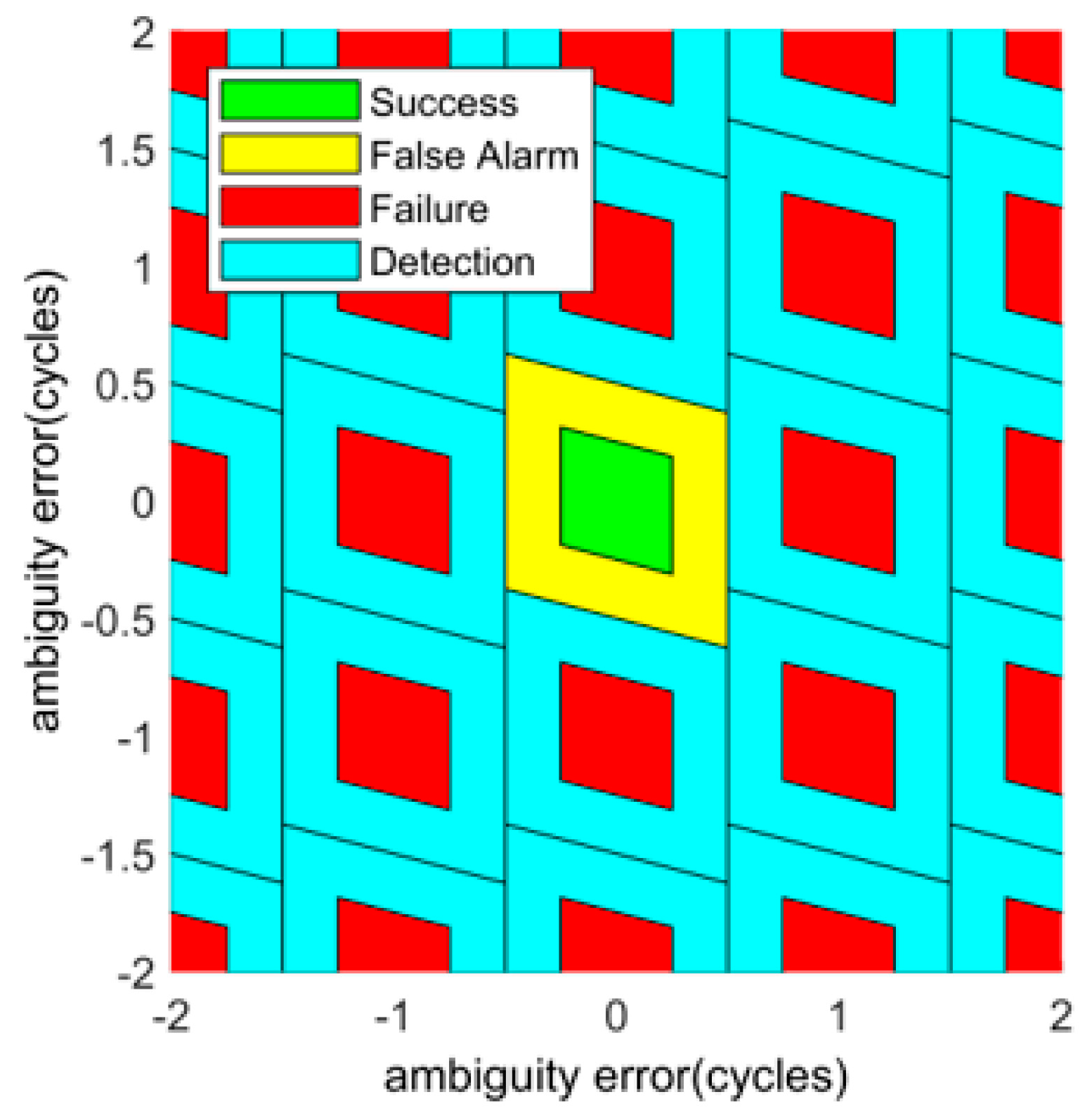
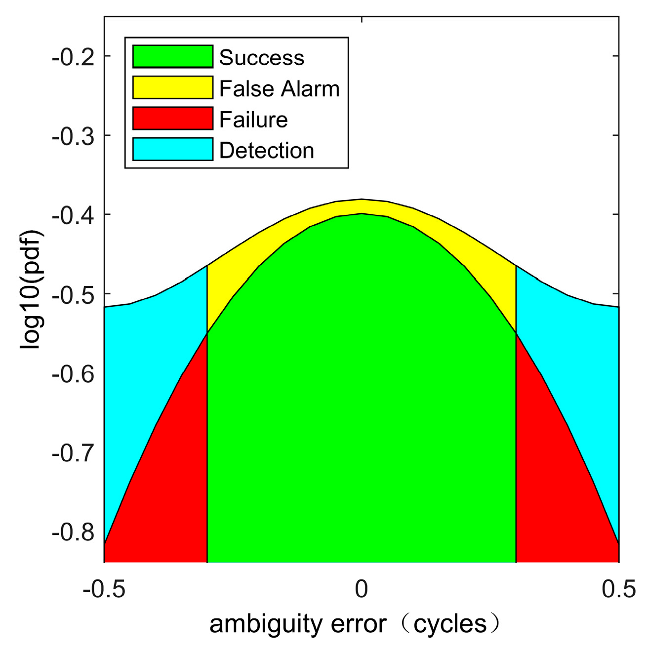
In this section, a simplified failure rate upper bound function of the aperture parameter is derived on the hypothesis of weak correlation of the decorrelated ambiguities. Then, the probabilities of the other events are analyzed based on this simplified function.

3.1. IAB Events

IAB has four mutually exclusive and independent outcome events (success, failure, false alarm, and detection) [30,31]. The success event, H S , occurs upon acceptance of the correct integer, the failure event, H F , occurs upon acceptance of any incorrect integers, the false-alarm event, H E , occurs upon rejection of the correct integer, and the detection event, H D , occurs upon rejection of any incorrect integer. Let ϵ = z ^ I B z ˙ be the vector of the float ambiguity error. The regions corresponding to H S , H F , H E , and H D events are illustrated in Figure 1.

3.2. Simplified Function to Compute the Upper Bound of Failure Rate
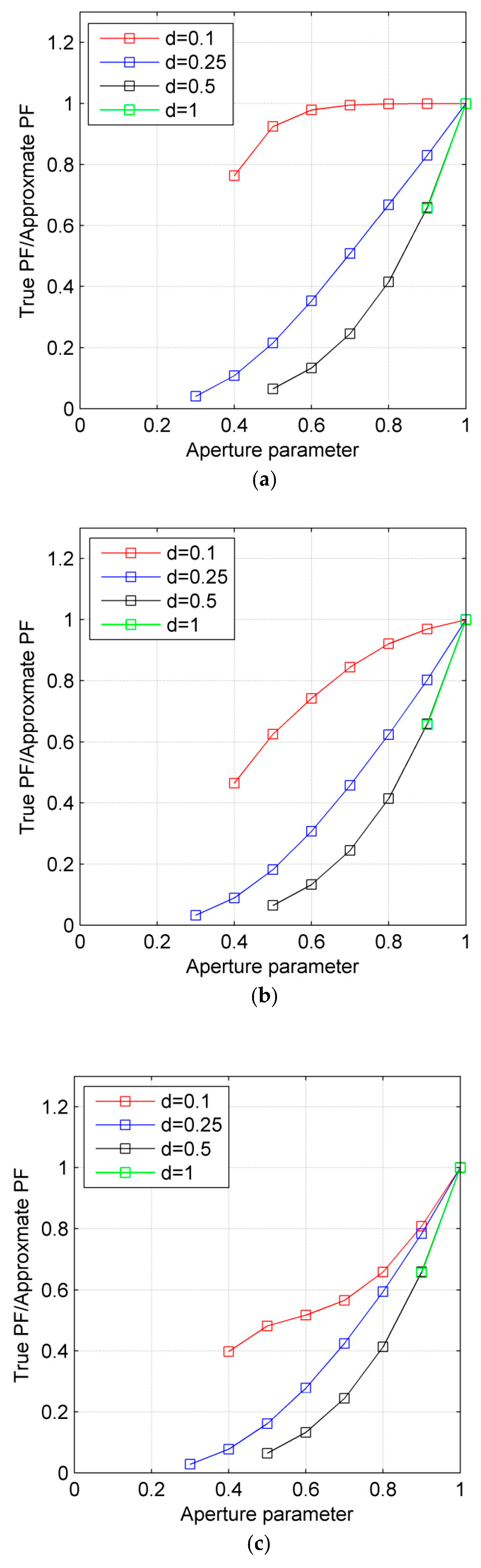
The failure event probability, termed the failure rate, is an important integrity parameter. IAB has the advantage that its failure rate can be computed and controlled by the aperture parameter, K , as follows.
Let Δ z = z ˇ I B z ˙ be the vector of the integer ambiguity error, and the probability of the acceptance of the ambiguity with integer error, Δ z , is given as [22]:
P ( Δ z | I A B ) = i = 1 n ( Φ ( k i 2 L i Δ z 2 d i ) Φ ( k i 2 L i Δ z 2 d i ) )
where L i is the i-th row of L .
The failure rate, P F , is the probability of acceptance of all the incorrect integers [22], as:
P F = P ( H F ) = Δ z 0 n   a n d     Δ z Z n       P ( Δ z | I A B ) = Δ z 0 n   Δ z Z n       i = 1 n ( Φ ( k i 2 L i Δ z 2 d i ) Φ ( k i 2 L i Δ z 2 d i ) )
Since (12) contains an infinite number of items, it is impossible to compute the true value of P F . However, a precise estimation of P F can be obtained by calculating only the: i = 1 n ( Φ ( k i 2 L i Δ z 2 d i ) Φ ( k i 2 L i Δ z 2 d i ) ) , with a high probability.
The computations of (12) may be complex with a weak CDGNSS model. In our study, a probability estimation based on weak correlation is proposed to reduce the computational complexity, as follows.
The P F can be expressed as:
  P F = Δ z Z n P ( Δ z | I A B ) P ( 0 n | I A B )  
Clearly, P F can be easily obtained as Δ z Z n P ( Δ z | I A B ) is calculated.
On the hypothesis of a weak correlation of decorrelated ambiguities, Δ z and Δ z i are related by L i as:
  L i Δ z Δ z i
where Δ z i denotes the i-th integer element of Δ z .
Then, Δ z Z n P ( Δ z | I A B ) can be expressed as:
Δ z Z n P ( Δ z I A B ) = Δ z Z n i = 1 n ( Φ ( k i 2 L i Δ z 2 d i ) Φ ( k i 2 L i Δ z 2 d i ) ) Δ z Z n i = 1 n ( Φ ( k i 2 Δ z i 2 d i ) Φ ( k i 2 Δ z i 2 d i ) ) = i = 1 n Δ z i Z 1 ( Φ ( k i 2 Δ z i 2 d i ) Φ ( k i 2 Δ z i 2 d i ) ) = i = 1 n l Z 1 ( Φ ( k i 2 l 2 d i ) Φ ( k i 2 l 2 d i ) )
Let F i ( k i ) = l Z 1 ( Φ ( k i 2 l 2 d i ) Φ ( k i 2 l 2 d i ) ) and F i , j ( k i ) = Φ ( k i 2 l 2 d i ) Φ ( k i 2 l 2 d i ) , then:
Δ z Z n P ( Δ z | I A B ) = i = 1 n F i ( k i )
P ( 0 n | I A B ) = i = 1 n F i , 0 ( k i )
P F = i = 1 n F i ( k i ) i = 1 n F i , 0 ( k i )
The calculation of F i ( k i ) is not possible directly due to its infinite number of items. However, an approximate value can be calculated as follows:
F i ( k i ) = l Z 1 F i , l ( k i ) = l [ N : N ] F i , l ( k i ) + l [ : N 1 ] F i , l ( k i ) + l [ N + 1 : ] F i , l ( k i )
Thus,
l [ : n 1 ] F i , l ( k i ) = l [ n + 1 : ] F i , l ( k i ) < Φ ( k i 2 N + 2 2 d i )
l [ N : N ] F i , l ( k i ) + 2 Φ ( k i 2 N + 2 2 d i ) F i ( k i ) l [ N : N ] F i , l ( k i )
The upper and lower bounds on F i ( k i ) can be accurately estimated according to the formula, and the estimated error range can be determined by 2 Φ ( k i 2 N + 2 2 d i ) . Conservatively, an upper bound on the failure rate can be expressed as:
P F = i = 1 n F i ( k i ) i = 1 n F i , 0 ( k i ) = i = 1 n l [ N : N ] ( Φ ( k i 2 l 2 d i ) Φ ( k i 2 l 2 d i ) ) + 2 Φ ( k i 2 N + 2 2 d i ) i = 1 n ( Φ ( k i 2 d i ) Φ ( k i 2 d i ) )
Compared to (12), (19) can drastically reduce the amount of computation by exchanging the order of addition and multiplication.
To validate the simplified function for the failure rate, we compared the true P F value obtained by (12) with the correlation matrix, L , the conditional-variance matrixes, D , and the aperture parameter, K , in two dimensions, with the approximate P F values obtained by (19), where L = [ 1 0 l 1 , 2 1 ] , D = [ d 0 0 d ] , and K = [ k k ] . It can be found in Figure 2 that:
(a)
The approximate P F is always higher than the true P F , so the simplified function (19) can obtain the upper bound on the failure rate.
(b)
The accuracy of the approximation of the failure rate is proportional to the aperture parameter value and inversely proportional to the conditional variance value and correlation value, with the range of the correlation value being 0 to 0.5.

3.3. Probabilities of the Other IAB Events

The probability of a success event, H S , denoted as P S , can be expressed as:
P S = P ( H S ) = P ( 0 n | I A B ) = i = 1 n ( Φ ( k i 2 d i ) Φ ( k i 2 d i ) )
The probability of a false-alarm event, H E , denoted as P E , can be expressed as:
P E = P ( H E ) = P ( 0 n | I B ) P ( 0 n | I A B ) = i = 1 n ( Φ ( 1 2 d i ) Φ ( 1 2 d i ) ) i = 1 n ( Φ ( k i 2 d i ) Φ ( k i 2 d i ) )
where P ( 0 n | I B ) is the probability of fixing the correct integer ambiguity in IB.
As P S , P E , and P F can be computed, the probability of detection event, H D , denoted as P D , can be expressed as:
P D = P ( H D ) = 1 P S P E P F
The fix rate, denoted as P A , is the probability of the fix event occurring upon acceptance of any integer. P A can be expressed as:
P A = P S + P E
In addition to the above parameters, the following two conditional probabilities are usually used in integrity:
(a)
The missing detection rate, P M D , is the conditional probability of a failure event given the event that occurs upon acceptance of any integer:
P M D = P ( H F | ( H F + H S ) ) = P F P S + P F
(b)
The false-detection rate, P F D , is the conditional probability of a false-alarm event given the event that occurs upon rejection of any integer:
P F D = P ( H E | ( H E + H D ) ) = P E P E + P D

4. AIAB Optimal Aperture Shape Based on the Upper Bound on the Failure Rate

This section derives a constraint function to describe the optimized aperture relationship that determines the AIAB aperture shape. The constraint function is then simplified to reduce computational complexity.

4.1. The AIAB Constraint Function

IAB is an integrity-monitoring method that aims to reduce the integrity risk by increasing the availability risk. Figure 3 shows that although the false-alarm rate increased, the failure rate decreased in IAB.
The optimal IAB aperture parameter should provide the lowest false-detection rate for a given missed detection rate, P M D , a l l o c , as:
a r g   m i n [ P F D ] s . t . P M D = P M D , a l l o c
where P F D = i = 1 n F 0 , i ( 1 ) i = 1 n F 0 , i ( k i ) i = 1 n F 0 , i ( 1 ) = 1 i = 1 n F 0 , i ( k i ) i = 1 n F 0 , i ( 1 ) and P M D = i = 1 n F i ( k i ) i = 1 n F 0 , i ( k i ) i = 1 n F i ( k i ) = 1 i = 1 n F 0 , i ( k i ) i = 1 n F i ( k i ) .
Equation (26) can be equated as:
a r g   m a x [ i = 1 n F 0 , i ( k i ) ] s . t .       i = 1 n F 0 , i ( k i ) i = 1 n F i ( k i ) = 1 P m d , a l l o c
The Lagrange multiplier calculator is used to locate the maxima of the function i = 1 n F 0 , i ( k i ) that is subject to i = 1 n F 0 , i ( k i ) i = 1 n F i ( k i ) = 1 P m d , a l l o c , as follows.
The formula of the Lagrange multiplier is:
L ( k 1 , , k n , λ ) = i = 1 n F 0 , i ( k i ) + λ ( i = 1 n F 0 , i ( k i ) i = 1 n F i ( k i ) 1 + P m d , a l l o c )
Set the gradient of L ( k 1 , , k n , λ ) equal to the zero vector as:
L ( k 1 , , k n , λ ) k j = f 0 , j ( k j ) F 0 , j ( k j ) i = 1 n F 0 , i ( k i ) + λ f 0 , j ( k j ) F 0 , j ( k j ) i = 1 n F 0 , i ( k i ) f j ( k j ) F j ( k j ) i = 1 n F 0 , i ( k i ) i = 1 n F i ( k i ) = 0
Equation (29) can be simplified as:
1 λ i = 1 n F i ( k i ) 1 = f j , 0 ( k j ) / f j ( k j ) F j , 0 ( k j ) / F j ( k j )
Finally, the optimal IAB aperture parameter relationship can be obtained as:
F i , 0 ( k i ) / F i ( k i ) f i , 0 ( k i ) / f i ( k i ) = F j , 0 ( k j ) / F j ( k j ) f j , 0 ( k j ) / f j ( k j )
where i and j denote the subscripts corresponding to the integer ambiguities.
Similarly, it can be proven that Equation (31) also satisfies the following:
(a)
Subject to a given fix rate or a given success rate, locate the minimum of the false-alarm rate, false-detection rate, missed detection rate, and failure rate.
(b)
Subject to a given false-alarm rate or a given false-detection rate, locate the minimum of the missed detection rate and failure rate and the maximum of the fix rate and success rate.
(c)
Subject to a given missed detection or a given failure rate, locate the minimum of the false-alarm rate and failure rate, and the maximum of the fix rate and success rate.
It can be seen that (31) provides the optimal aperture shape under weak correlation assumptions of the integer ambiguities.
Therefore, the AIAB constraint function can be defined as:
R b a s i c ( k i , d i ) = F i , 0 ( k i ) / F i ( k i ) f i , 0 ( k i ) / f i ( k i )
The function is also called the basic R-value function. Let the (32) function value be the R-value. As can be seen from Figure 4, for a given value of d , the R-value is monotonically increasing with the aperture parameter, which implies that there is a one-to-one correspondence between the R-value and the aperture parameter. The range of the R-value is 1 to F i , 0 ( 1 i ) / F i ( 1 ) f i , 0 ( 1 ) / f i ( 1 ) , where F i , 0 ( 1 i ) / F i ( 1 ) f i , 0 ( 1 ) / f i ( 1 ) < 2 and F i , 0 ( 1 i ) / F i ( 1 ) f i , 0 ( 1 ) / f i ( 1 ) is inversely proportional to d .
The key of AIAB is to let the R-value of different integer ambiguities be the same, but it needs to take into account the range of the R-value. When the R-value exceeds its maximum value range, the corresponding aperture parameter is set to 1.

4.2. The Simplified AIAB Constraint Function

The calculation and inversion of the R-value function (32) is very complex and can be considered to simplify it. As F i , 0 ( k i ) and F i ( k i ) are less sensitive than f i , 0 ( k i ) and f i ( k i ) to the aperture parameter with F i , 0 ( k i ) / F i ( k i ) 1 , the simplified R-value function can be expressed as:
R f / f 0 ( k i , d i ) = 1 f i , 0 ( k i ) / f i ( k i ) = f i ( k i ) / f i , 0 ( k i )
The simplified R-value function is compared with other simplified functions, as follows:
R F 0 / F ( k i , d i ) = F i , 0 ( k i ) / F i ( k i )
R F 0 / f 0 ( k i , d i ) = F i , 0 ( k i ) / f i , 0 ( k i )
Similarly, the R-value function of the Basic IAB can be defined as:
R B a s i c I A B ( k i , d i ) = k i  
The above R-values were normalized by R b a s i c to compare the similarity with the AIAB basic constraint function in Figure 5a,b. It is shown that the similarity between the R f / f 0 and R b a s i c was the highest in both strong and weak CDGNSS models. However, the similarity slightly decreased in the weak GNSS model. Additionally, R B a s i c I A B exhibited the lowest similarity to R b a s i c .
The R f / f 0 function (33a) can be further simplified as follows:
(a)
f i , 0 ( k i ) can be expressed as:
f i , 0 ( k i ) = p d f n o r m ( 0.5 k i d i ) + p d f n o r m ( 0.5 k i d i ) 2 = 1 2 π d i e x p ( 1 2 ( k i 2 d i ) 2 )
where p d f n o r m denotes the normal probability density function formula.
(b)
f i ( k i ) can be expressed as:
f i ( k i ) = , l Z 1 f i , l ( k i ) f i , 0 ( k i ) + f i , 1 ( k i ) + f i , 1 ( k i ) = 1 2 π d i exp ( 1 2 ( k i 2 d i ) 2 ) + 1 2 π d i exp ( 1 2 ( 2 k i 2 d i ) 2 ) + 1 2 π d i exp ( 1 2 ( 2 + k i 2 d i ) 2 )
As 1 2 π d i exp ( 1 2 ( 2 + k i 2 d i ) 2 ) 1 2 π d i e x p ( 1 2 ( 2 k i 2 d i ) 2 ) , f i ( k i ) can be simplified as:
f i ( k i ) exp ( 1 2 ( k i 2 d i ) 2 ) + exp ( 1 2 ( 2 k i 2 d i ) 2 )
(c)
R f / f 0 can be simplified as:
f i , 0 ( k i ) f i ( k i ) exp ( 1 2 ( k i 2 d i ) 2 ) exp ( 1 2 ( k i 2 d i ) 2 ) + exp ( 1 2 ( 2 k i 2 d i ) 2 ) = 1 1 + exp ( 1 2 ( 2 k i 2 d i ) 2 + 1 2 ( k i 2 d i ) 2 )
The constraint function becomes ( 2 k i 2 d i ) 2 + ( k i 2 d i ) 2 = k j 1 d j 2 . Let the simplified R f / f 0 be R d d , as:
R d d ( k i , d i ) = k i 1 d i 2
Compared to the complexity of solving and inverting the R b a s i c function, the computational complexity of solving and inverting R d d was greatly reduced. Therefore, this constraint function can be called the AIAB-DD constraint function, while the original basic AIAB constraint function is called the AIAB-Basic constraint function.

5. Setting AIAB Aperture Size with Data Constraint

This section provides a detailed description of a new IAB approach aimed at avoiding the computational complexity associated with using the fixed failure rate (FF) approach.

5.1. AIAB Approach with Performance Constraint

Currently, the aperture parameter is determined using the FF approach. This approach is essentially a method of performance constraint that determines the aperture parameters based on performance requirements, such as the failure rate, and then compares the ambiguity residuals with the aperture parameters to decide whether the performance requirement can be met. The AIAB approach with the performance constraint can be performed by the Monte Carlo method or the following steps, as:
(a)
As the relationship between R d d and the failure rate can be obtained from (12), (19), and (38), R d d can be estimated by a dichotomy search or other methods for a given failure rate.
(b)
If R d d is known, the aperture parameter can be solved by (38).
Clearly, the computational complexity of the AIAB approach with the performance constraint is extremely high due to the search of R d d .

5.2. AIAB Approach with Data Constraint

Unlike the approach with the performance constraint, the AIAB approach with the data constraint determines the aperture parameter by the AIAB-DD constraint function based on the ambiguity residuals and then calculates the performance parameter, such as the failure rate, and compares the calculated performance parameter with the allocated performance parameter to determine whether the performance requirement is met. Taking the failure rate as an example of the performance parameter, the AIAB approach with the data constraint is shown in Figure 6. The failure rate was firstly computed by the simplified function (21) to reduce computational complexity, and secondly computed (if needed) by (14) to avoid the performance losses. In most cases, the failure rate only needs to be calculated once. It should be noted that the input parameter can be the missed detection rate, the false-alarm rate, etc. This is another advantage over the approach with the performance constraint.
It can be seen that the greatest computational complexity in AIAB lies in the possible second failure rate calculation. Further, the Simplified AIAB has been proposed by removing the second failure rate calculation in Figure 6 to meet the requirements of practical engineering applications.
In summary, AIAB can be implemented by either a performance-constraint-based class FF approach or a data-constraint-based approach. Compared to the FF-like AIAB method, the data-constrained AIAB method has a lower computational complexity. To verify this speculation, we conducted a comparison of the two computational complexities based on a MATLAB program on a Lenovo XI laptop with an i7-10510U CPU and 16 G of RAM for a total of 286 tests. The results showed that the average processing time of the data-constrained AIAB approach was 18.8 ms, and that of the performance-constrained FF-like AIAB approach was 291.3 ms. It can be seen that the running time of the data-constrained AIAB method was significantly lower than that of the FF-like method, and it can meet the requirements of engineering applications. Of course, the FF-like performance constraint approach also has certain advantages, which can provide clear thresholds and help to comprehensively analyze the performance. The data-constrained approach can only judge whether the current data meet a single performance requirement.

6. Simulations and Discussion

Simulations were conducted to verify the performance of AIAB and compare it with that of different IAB methods in two aspects: the global CDGNSS service performance simulation and the Monte Carlo simulation based on certain epochs.

6.1. The Global CDGNSS Service Performance Simulation

6.1.1. The Simulation Strategy

To demonstrate the projected AIAB performance in general, we conducted a series of simulations to compare AIAB with existing IAB methods, i.e., Basic IAB and GIAB. A simulated GPS constellation with 24 MEO was used to simulate and implement global L1C/A-based CDGNSS in the future Ground-Based Augmentation System (GBAS) for 24 h with a sampling interval of 3600 s, and the CDGNSS positioning was implemented worldwide, uniformly, with a 15-degree interval in both longitude and latitude. A total of eight parameter configurations in Table 1 were used to simulate as many different application scenarios as possible. Since GIAB determines the aperture parameter by the failure rate, the failure rate was chosen to compare the different methods. The required integrity risk was set as 2 × 10⁻⁷ in the landing of aircraft and autonomous driving of land vehicles, and the corresponding required failure rate was allocated as 10−8. Therefore, the failure rate was configured to 10−8 and 10−4 for high-integrity and middle-integrity applications, respectively. The undifferentiated observation noise of a single differential code between the base station and the rover was simulated to follow a normal distribution, with σ Δ ρ of 0.1 m, 0.25 m, 0.5 m, and 1.0 m, respectively, so as to represent different CDGNSS models, and the undifferentiated observation noise of a single differential carrier phase at the base station and the rover was simulated to follow a normal distribution, with σ Δ α of 2 mm. The number of fixed ambiguities was set to 4 to fairly compare the different methods. Therefore, a total of 507,264 scenarios with different failure rates and model strengths were simulated to evaluate the performance of the AIAB as comprehensively as possible. When using the Monte Carlo method to validate performance, each scenario needs to be tested at least an order of magnitude higher than the inverse of the failure rate, and for a failure rate of 10−4, each scenario needs to be simulated 105 times, which is much longer than the computational power of our simulation equipment. As mentioned in Section 5, the FF-like approach can be used for the full performance evaluation, so we adopted the FF-like approach, as described in Section 5.1, to reduce the computational effort of the simulation by determining the threshold value based on the failure rate and then calculating other parameters, such as the fix rate. It should be noted that this is only for the purpose of comparing the performance, and the data-constrained AIAB method is still recommended for real applications.

6.1.2. The Comparison of Actual Failure Rates of Different Methods

The failure rate can be calculated by the GIAB failure rate function (9), the simplified function (19), and the basic function (20). Function (20) yields the true value of the failure rate, while functions (9) and (19) can only estimate its approximate upper bound value. Therefore, we can evaluate the accuracy of functions (9) and (19) by function (20).
First, it was verified that the simplified function (19) proposed in this paper can calculate an upper bound on the failure rate with the simplified AIAB aperture parameter from Scheme A1 to A8. The approximation function failure rate estimation accuracy has already been analyzed in Section 3.2 in relation to the aperture parameters and correlation coefficients. This section will focus on analyzing the estimation accuracy for different schemes. Let the simplified function be P FS and the true failure rate value of the basic function be P F , and the results are shown in Table 2. It can be seen that the P F was always less than P FS , implying that the failure rate of the simplified function can bound the true failure rate value and will not cause the integrity risk. Furthermore, the P F / P FS values for schemes A1, A2, A3, and A4 with a demanding failure rate of 10−4 were 0.91, 0.8, 0.73, and 0.66, respectively, showing that the weaker the model strength, the worse the estimation accuracy. Meanwhile, the P F / P FS values for schemes A1 and A5 were 0.91 and 0.81, respectively, showing that the lower the failure rate requirement, the better the estimation accuracy.
Second, the accuracy of the failure rate estimation was compared between the GIAB function (9) and the function (19) proposed in this paper. We examined the actual failure rates at various fix rates to compare the two failure rate approximation estimate functions, since the fix rate, to some extent, reflects the demanding failure rate and model strength. As shown in Figure 7, the true failure rates of the two methods did not exceed the configured failure rate, and the proposed function (19) provided a closer approximation to the true failure rate than GIAB, especially at low fix rates. Since the accuracy of the GIAB failure rate estimation significantly deteriorated at low fix rates and the performance of the IAB was mainly determined by the shape of the IAB and the failure rate, the performance of the GIAB decreased at low fix rates, as will be verified in the following.

6.1.3. The comparison of AIAB, GIAB, and the Basic IAB

Since the IAB method aims to obtain a higher fix rate with a set fixed failure rate, the fix rate was chosen as an indicator for comparing the performance of AIAB, Simplified AIAB, GIAB, and Basic IAB, as shown in Figure 8 and Table 3. The fix rates of AIAB, Simplified AIAB, GIAB, and Basic IAB are denoted as P A _ AIAB , P A _ SAIAB , P A _ GIAB , and P A _ BIAB , respectively. According to the P A _ BIAB , the results were divided into four categories: low, medium, high, and very high, corresponding to the range of P A _ BIAB equal to [0.2–0.6), [0.6–0.9), [0.9–0.95), and [0.95–1], respectively. AIAB had the highest fix rate, and Simplified AIAB was second only to AIAB. In the case of the very high fix rate, the fix rates of the four methods were almost the same and were not listed in Table 3. In the case of the high fix rate, the fix rates of AIAB and Simplified AIAB were slightly higher than those of GIAB and Basic IAB. In the case of the low and middle fix rates, the fix rate of AIAB and Simplified AIAB was significantly higher than that of GIAB and Basic IAB.
The fix rate of the IAB is jointly affected by the model strength, the IAB threshold parameter relationship, and the failure rate. The model strengths of the four methods in the simulation were similar with the same simulation schemes. When the model strength was sufficient, the fix rates of the four methods were almost the same. As the model strength became weaker, the difference in fix rates between the four methods became larger due to the larger role of the other two factors in the fix rate of IAB. The failure rate was estimated by the basic function (20) in AIAB, by the proposed function (19) in Simplified AIAB and Basic IAB, and by the GIAB function (9) in GIAB. It is clear that AIAB had the highest fix rate due to its estimable, almost true failure rate and its more rational assignment of threshold parameters. Although Simplified AIAB and IAB use the same failure rate estimation function, the lower fix rate in IAB than in Simplified AIAB is due to the oversimplification of setting the threshold in IAB to the same value. GIAB virtually always beats basic IAB in fix rate, but the plots in Figure 8 and Table 3 show that GIAB was frequently worse than IAB in the case of a high fix rate. Although GIAB had a more reasonable constraint relationship for the aperture parameters than IAB, the accuracy of the failure rate calculation of GIAB by (9) was lower than that of IAB by (19), which is the main reason why GIAB will perform worse than IAB in the case of a low fix rate.

6.2. The Monte Carlo Simulation

It is well known that the state-of-the-art Optimal Integer Aperture (OIA) [16] is the theoretically best IA method, but its threshold value can only be determined accurately by Monte Carlo methods. To further demonstrate the performance of AIAB, a Monte Carlo test was implemented to compare the performance of AIAB with OIA. It has been shown in Section 6.1 that there is a difference in the effectiveness of different IA methods in the case of insufficient model strength. Therefore, the ambiguity covariance matrix, Q a , which is [   6.2900 ,   5.9780 , 0.5440 ; 5.9780 ,   6.2920 ,   2.3400 ; 0.5440 ,   2.3400 ,   6.2880 ] , in ambiguity success rate evaluation software, Ps-lambda [32], was chosen to be multiplied by a factor of 0.0095 so that its fix rate without IA is equal to 0.9 in order to make the model strength suitable for comparing the failure rate of AIAB with OIA at the same fix rate. As shown in Figure 9a, the failure rate of AIAB was almost the same as that of OIA. Meanwhile, the simulation epoch in Section 6.1 was randomly selected to compare the difference in failure rates between OIA and AIAB using the same methodology, and as shown in Figure 9b. The failure rate for AIAB was slightly higher than OIA by less than 20% to 40%, with the difference controlled within reasonable limits. The results show that AIAB can yield almost theoretically the best IA performance.

7. Conclusions

In order to solve the problem of the ambiguity fixation error, this paper has investigated the IAB issue, which provides resolved failure rates, in the ambiguity acceptance testing problem, and proposed a new method called AIAB, aiming to provide near-optimal IA aperture parameters. Unlike existing heuristic-based methods, the AIAB method is derived based on the optimization theory of IA and provides the highest success rate at a fixed failure rate, with an easy-to-compute function of the failure rate. Another advantage of AIAB is its ability to determine whether the current failure rate meets the requirements based on real-time data, rather than determining the threshold value based on the failure rate, which is computationally complex.
The performance of AIAB was tested by global CDGNSS simulations with different model strengths. The experimental results showed that the performance of different IABs was mainly determined by the strength of the model, the accuracy of the failure rate estimation, and the relationship between the thresholds of the IAB methods. When the model was not strong enough, AIAB had a higher fixation rate than the basic IAB method of GIAB due to its ability to estimate the actual failure rate and the fact that its threshold relationship is derived from the theoretical optimum. Furthermore, the performance advantage of AIAB became more apparent as the model strength decreased.
After verifying that the AIAB method is the optimal method of all the IABs, the theoretically optimal IA method, i.e., the OIA, was used to compare with the AIAB method via Monte Carlo simulation. The results showed that for the same fix rate, the true failure rate of the AIAB method was comparable to or slightly lower than that of OIA by 20% to 40%, proving that it has a performance close to the theoretical optimum.
In summary, AIAB has been proposed to provide superior performance of ambiguity acceptance tests than existing IAB methods with low computational complexity. However, similar to other IA methods, the performance of the AIAB method heavily depends on the accuracy of the underlying model used for the GNSS data. If the underlying model for AIAB does not match the characteristics of the real data, it may result in the AIAB failure rate exceeding the allocated value or the performance of AIAB being comparable to that of other IAB methods. For example, although difference testing has been shown to outperform ratio testing, in theory [33], ratio testing is even more robust to underlying model errors and, therefore, outperforms difference testing in real experiments [34]. The AIAB method, similar to most other IA methods, is limited to theoretical analyses and simulation validation due to the need for a large amount of historical data related to the application scenario to obtain accurate underlying models for real-world data. In the future, we will conduct research to construct the underlying model using historical data and correct it by combining observation residuals. This will allow us to carry out further methodological research and validation work of AIAB using real data. Finally, the AIAB needs to be developed for calculating position domain integrity risk to improve the availability of positioning services.

Author Contributions

Conceptualization, J.Z., P.H. and Y.W.; methodology, J.Z.; software, J.Z. and C.S.; validation, J.Z. and L.W.; formal analysis, Q.Y. and L.W.; investigation, J.Z. and J.Y.; writing—original draft preparation, J.Z. and P.H.; writing—review and editing, J.Z., P.H., C.S. and L.W.; supervision, B.Y.; project administration, B.Y.; funding acquisition, B.Y. and J.Y. All authors have read and agreed to the published version of the manuscript.

Funding

This research was supported by the State Key Laboratory of Satellite Navigation System and Equipment Technology (Grant No. 22684X023) and Hebei province key research and development project “Navigation positioning and 5G communication multi-mode integration of key technologies” (20310901D).

Data Availability Statement

No new data were created or analyzed in this study. Data sharing is not applicable to this article.

Conflicts of Interest

The authors declare no conflicts of interest.

References

  1. Rife, J.; Khanafseh, S.; Pullen, S.; De Lorenzo, D.; Kim, U.-S.; Koenig, M.; Chiou, T.-Y.; Kempny, B.; Pervan, B. Navigation, Interference Suppression, and Fault Monitoring in the Sea-Based Joint Precision Approach and Landing System. Proc. IEEE 2008, 96, 1958–1975. [Google Scholar] [CrossRef]
  2. Joerger, M.; Spenko, M. Towards Navigation Safety for Autonomous Cars. Inside GNSS 2017, 40–49. Available online: https://par.nsf.gov/biblio/10070277 (accessed on 15 July 2022).
  3. Sassi, I.; El-Koursi, E.-M. On-board train integrity: Safety requirements analysis. In Proceedings of the 29th European Safety and Reliability Conference (ESREL), Hannover, Germany, 22–26 September 2019. [Google Scholar]
  4. Urquhart, L.; Leandro, R.; Gonzales, P. Integrity for high accuracy GNSS correction services. In Proceedings of the 2019 International Technical Meeting of The Institute of Navigation, Reston, Virginia, 28–31 January 2019; pp. 543–553. [Google Scholar]
  5. Khanafseh, S.; Pervan, B. New Approach for calculating position domain integrity risk for cycle resolution in carrier phase navigation systems. IEEE Trans. Aerosp. Electron. Syst. 2010, 46, 296–307. [Google Scholar] [CrossRef]
  6. Wu, S.; Peck, S.R.; Fries, R.M.; McGraw, G.A. Geometry extra-redundant almost fixed solutions: A high integrity approach for carrier phase ambiguity resolution for high accuracy relative navigation. In Proceedings of the 2008 IEEE/ION Position, Location and Navigation Symposium, Monterey, CA, USA, 5–8 May 2008; pp. 568–582. [Google Scholar]
  7. Khanafseh, S.; Pervan, B. Detection and mitigation of reference receiver faults in differential carrier phase navigation systems. IEEE Trans. Aerosp. Electron. Syst. 2011, 47, 2391–2404. [Google Scholar] [CrossRef]
  8. Teunissen, P.J.G. Success probability of integer GPS ambiguity rounding and bootstrapping. J. Geod. 1998, 72, 606–612. [Google Scholar] [CrossRef]
  9. Teunissen, P.J. Integer aperture GNSS ambiguity resolution. Artif. Satell. 2003, 38, 79–88. [Google Scholar]
  10. Han, S. Quality-control issues relating to instantaneous ambiguity resolution for real-time GPS kinematic positioning. J. Geod. 1997, 71, 351–361. [Google Scholar] [CrossRef]
  11. Teunissen, P.J.G. An optimality property of the integer least-squares estimator. J. Geod. 1999, 73, 587–593. [Google Scholar] [CrossRef]
  12. Chang, X.-W.; Yang, X.; Zhou, T. MLAMBDA: A modified LAMBDA method for integer least-squares estimation. J. Geod. 2005, 79, 552–565. [Google Scholar] [CrossRef]
  13. Giorgi, G.; Teunissen, P.J.G. Carrier phase GNSS attitude determination with the Multivariate Constrained LAMBDA method. In Proceedings of the 2010 IEEE Aerospace Conference, Big Sky, MT, USA, 6–13 March 2010; pp. 1–12. [Google Scholar]
  14. Verhagen, S.; Teunissen, P.J.G. New Global Navigation Satellite System Ambiguity Resolution Method Compared to Existing Approaches. J. Guid. Control Dyn. 2006, 29, 981–991. [Google Scholar] [CrossRef]
  15. Teunissen, P.; Verhagen, S. The GNSS ambiguity ratio-test revisited: A better way of using it. Surv. Rev. 2009, 41, 138–151. [Google Scholar] [CrossRef]
  16. Teunissen, P.J. GNSS ambiguity resolution with optimally controlled failure-rate. Artif. Satell. 2005, 40, 219–227. [Google Scholar]
  17. Verhagen, S.; Teunissen, P.J. The ratio test for future GNSS ambiguity resolution. GPS Solut. 2012, 17, 535–548. [Google Scholar] [CrossRef]
  18. Wang, L.; Verhagen, S. A new ambiguity acceptance test threshold determination method with controllable failure rate. J. Geod. 2014, 89, 361–375. [Google Scholar] [CrossRef]
  19. Hou, Y.; Verhagen, S.; Wu, J. An efficient implementation of fixed failure-rate ratio test for gnss ambiguity resolution. Sensors 2016, 16, 945. [Google Scholar] [CrossRef] [PubMed]
  20. Teunissen, P.J.G. The probability distribution of the ambiguity bootstrapped GNSS baseline. J. Geod. 2001, 75, 267–275. [Google Scholar] [CrossRef]
  21. Teunissen, P.J. GNSS ambiguity bootstrapping: Theory and applications. In Proceedings of the International Symposium on Kinematic Systems in Geodesy, Geomatics and Navigation, Banff, AB, Canada, 5–8 June 2001; pp. 246–254. [Google Scholar]
  22. Teunissen, P. Integer aperture bootstrapping: A new GNSS ambiguity estimator with controllable fail-rate. J. Geod. 2005, 79, 389–397. [Google Scholar] [CrossRef]
  23. Teunissen, P.J. A carrier phase ambiguity estimator with easy-to-evaluate fail-rate. Artif. Satell. 2003, 38, 89–96. [Google Scholar]
  24. Green, G.N.; King, M.; Humphreys, T. Data-driven generalized integer aperture bootstrapping for real-time high integrity applications. In Proceedings of the 2016 IEEE/ION Position, Location and Navigation Symposium (PLANS), Savannah, GA, USA, 11–14 April 2016; pp. 272–285. [Google Scholar]
  25. Green, G.N.; Humphreys, T.E. Data-driven generalized integer aperture bootstrapping for high-integrity positioning. IEEE Trans. Aerosp. Electron. Syst. 2019, 55, 757–768. [Google Scholar] [CrossRef]
  26. Green, G.N.; Humphreys, T. Position-domain integrity analysis for generalized integer aperture bootstrapping. IEEE Trans. Aerosp. Electron. Syst. 2019, 55, 734–746. [Google Scholar] [CrossRef]
  27. Li, L.; Li, Z.; Yuan, H.; Wang, L.; Hou, Y. Integrity monitoring-based ratio test for GNSS integer ambiguity validation. GPS Solut. 2016, 20, 573–585. [Google Scholar] [CrossRef]
  28. Teunissen, P.J.G. The least-squares ambiguity decorrelation adjustment: A method for fast GPS integer ambiguity estimation. J. Geod. 1995, 70, 65–82. [Google Scholar] [CrossRef]
  29. Crassidis, J.L.; Markley, F.L.; Lightsey, E.G. Global positioning system integer ambiguity resolution without attitude knowledge. J. Guid. Control Dyn. 2007, 30, 346–356. [Google Scholar] [CrossRef]
  30. Zhang, J.; Wu, M.; Li, T.; Zhang, K. Integer aperture ambiguity resolution based on difference test. J. Geod. 2015, 89, 667–683. [Google Scholar] [CrossRef]
  31. Liu, X.; Wang, Q.; Zhang, S.; Wu, S. A new efficient fusion positioning method for single-epoch multi-GNSS based on the theoretical analysis of the relationship between ADOP and PDOP. GPS Solut. 2022, 26, 139. [Google Scholar] [CrossRef]
  32. Verhagen, S.; Li, B.; Teunissen, P.J. Ps-LAMBDA: Ambiguity success rate evaluation software for interferometric applications. Comput. Geosci. 2013, 54, 361–376. [Google Scholar] [CrossRef]
  33. Li, T.; Zhang, J.; Wu, M.; Zhu, J. Integer aperture estimation comparison between ratio test and difference test: From theory to application. GPS Solut. 2016, 20, 539–551. [Google Scholar] [CrossRef]
  34. Wang, L.; Feng, Y.; Guo, J. Reliability control of single-epoch RTK ambiguity resolution. GPS Solut. 2016, 21, 591–604. [Google Scholar] [CrossRef]
Figure 1. Regions of the float ambiguity error, mapped by the IAB to success, failure, false-alarm, and detection events for a two-dimensional example model.
Remotesensing 16 00118 g001
Figure 2. True failure rate value vs. approximate failure rate value. (a) True P F value vs. approximate P F value, with a weak correlation value of l 1 , 2 = 0.1. (b) True P F value vs. approximate P F value, with a middle correlation value of l 1 , 2 = 0.3. (c) True P F value vs. approximate P F value, with a strong correlation value of l 1 , 2 = 0.5.
Remotesensing 16 00118 g002
Figure 3. Illustration of a one-dimensional integer aperture estimation model for the ambiguity validation problem.
Remotesensing 16 00118 g003
Figure 4. R-value with different aperture parameter values and d values.
Remotesensing 16 00118 g004
Figure 5. The similarity of simplified functions to the basic AIAB constraint function in the strong CDGNSS model, with d = 0.25 ( cycle ) and d = 1.0 ( cycle ) . (a) d = 0.25 ( cycle ) and (b) d = 1.0 ( cycle ) .
Remotesensing 16 00118 g005
Figure 6. The flowchart of the AIAB approach with the data constraint for a given failure rate, P F , a l l o c a t e d .
Remotesensing 16 00118 g006
Figure 7. The accuracy of the simplified failure rate function (PF_GIAB and PF_AIAB denote the true failure rate estimated by the GIAB function (9) and the proposed function (19), with the demanding failure rate being configured as PF).
Remotesensing 16 00118 g007
Figure 8. Comparison of the fix rate with Scheme A1 to A8. The points in the figure represent the epochs of the scheme, and the horizontal coordinates are the Basic IAB fix rate, Remotesensing 16 00118 i001 represents the AIAB fix rate, Remotesensing 16 00118 i002 represents the simplified AIAB fix rate, and Remotesensing 16 00118 i003 represents the GIAB fix rate. (a) The comparison of fix rate with Scheme A1. (b) The comparison of fix rate with Scheme A2. (c) The comparison of fix rate with Scheme A3. (d) The comparison of fix rate with Scheme A4. (e) The comparison of fix rate with Scheme A5. (f) The comparison of fix rate with Scheme A6. (g) The comparison of fix rate with Scheme A7. (h) The comparison of fix rate with Scheme A8.
Remotesensing 16 00118 g008
Figure 9. The comparison of OIA and AIAB failure rates. (a) The comparison with Q a = 0.0095 × [ 6.29 ,   5.98 ,   0.54 ;   5.98 ,   6.29 ,   2.34 ;   0.54 ,   2.34 ,   6.29 ] . (b) The comparison with the global simulation in Section 6.1.
Remotesensing 16 00118 g009
Table 1. The simulation strategy with a wide range of CDGNSS model parameters.
SchemePFσΔρ(m)
A110−40.1
A210−40.25
A310−40.5
A410−41.0
A510−80.1
A610−80.25
A710−80.5
A810−81.0
Table 2. The accuracy of the simplified failure rate function with different simulation schemes.
SchemeMaximum
(PF/PFS)
Mean
(PF/PFS)
Minimum
(PF/PFS)
A11.000.910.27
A21.000.800.22
A31.000.730.19
A41.000.660.21
A51.000.810.07
A61.000.650.07
A71.000.550.06
A81.000.470.07
Table 3. The comparison of fix rate with different simulation schemes.
P A _ B I A B Low (0.2 to 0.6)Medium (0.6 to 0.9)High (0.9 to 0.95)
Scheme P A _ A I A B P A _ B I A B P A _ S A I A B P A _ B I A B P A _ G I A B P A _ B I A B P A _ A I A B P A _ B I A B P A _ S A I A B P A _ B I A B P A _ G I A B P A _ B I A B P A _ A I A B P A _ B I A B P A _ S A I A B P A _ B I A B P A _ G I A B P A _ B I A B
A11.281.150.951.101.051.011.011.001.00
A21.291.120.881.101.031.001.011.001.00
A31.231.100.961.091.031.001.021.011.00
A41.261.070.861.081.021.001.021.011.00
A51.371.321.261.091.061.061.031.011.01
A61.381.241.151.121.061.041.031.011.01
A71.371.191.091.121.061.041.031.011.01
A81.401.171.021.171.051.031.031.011.00
Disclaimer/Publisher’s Note: The statements, opinions and data contained in all publications are solely those of the individual author(s) and contributor(s) and not of MDPI and/or the editor(s). MDPI and/or the editor(s) disclaim responsibility for any injury to people or property resulting from any ideas, methods, instructions or products referred to in the content.

