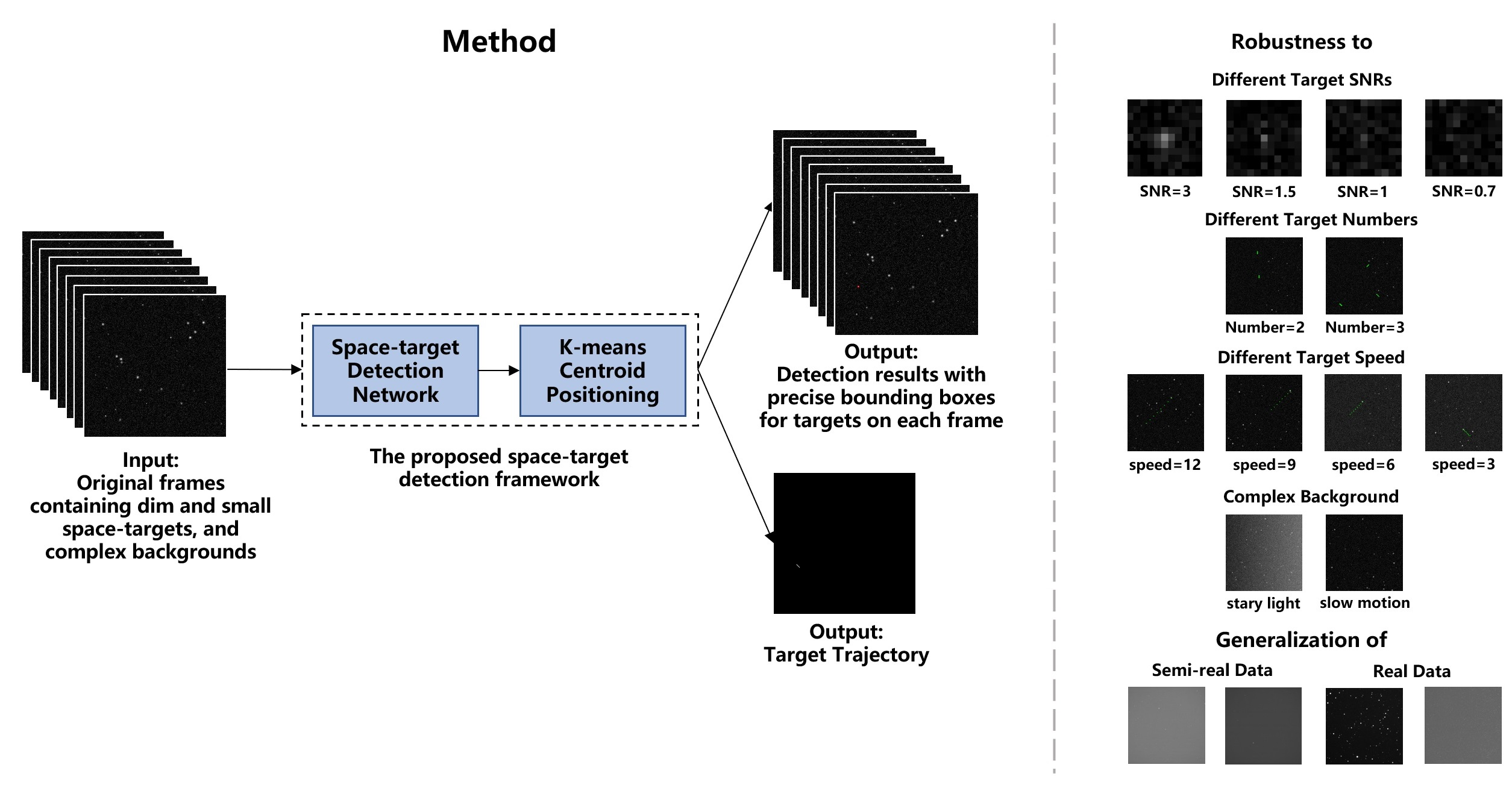
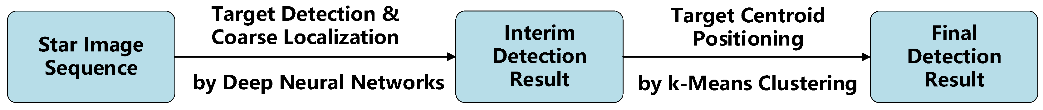
Figure 1.
Flow chart of the proposed dim and small space-target detection framework.
Figure 1.
Flow chart of the proposed dim and small space-target detection framework.
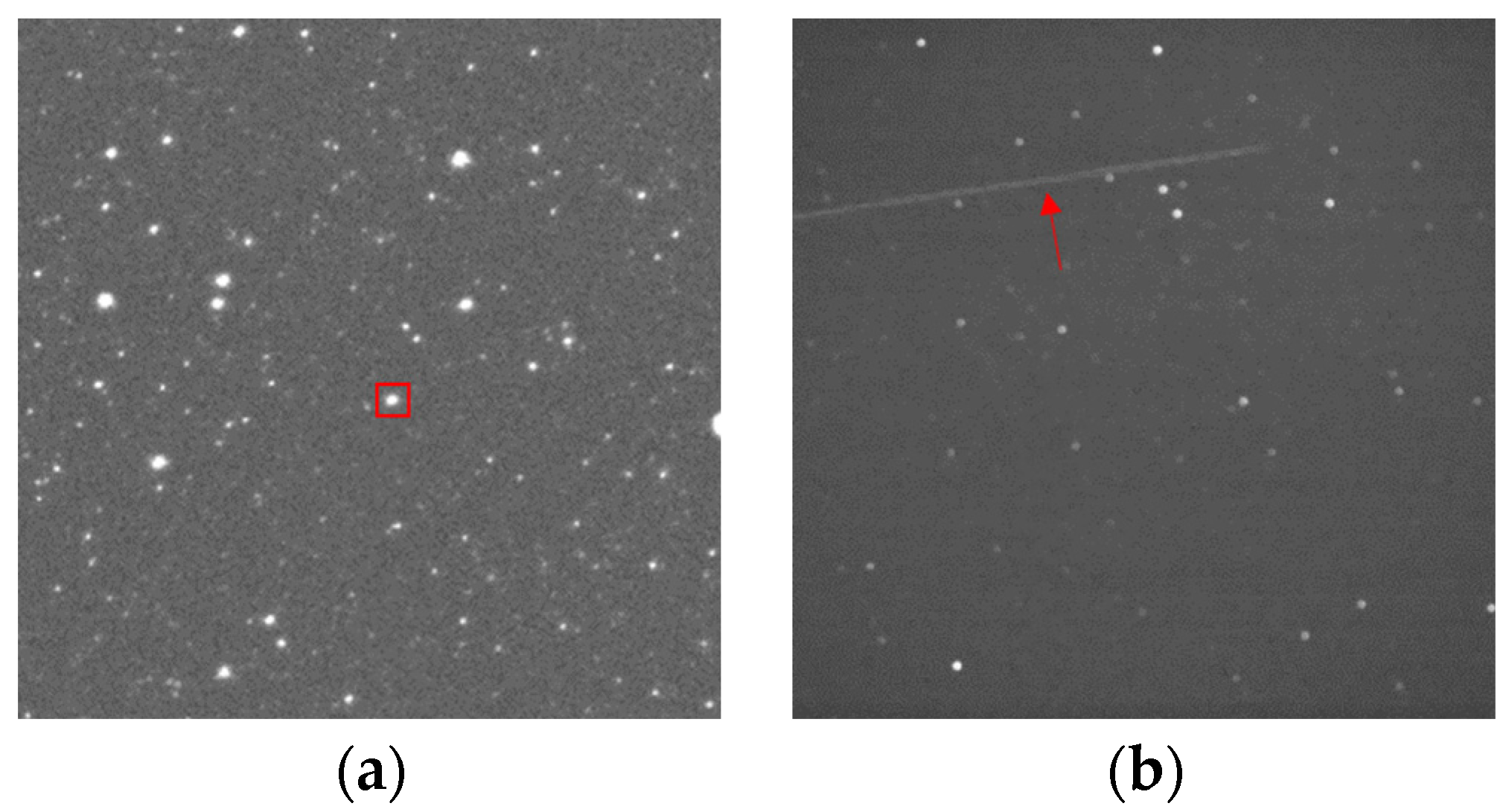
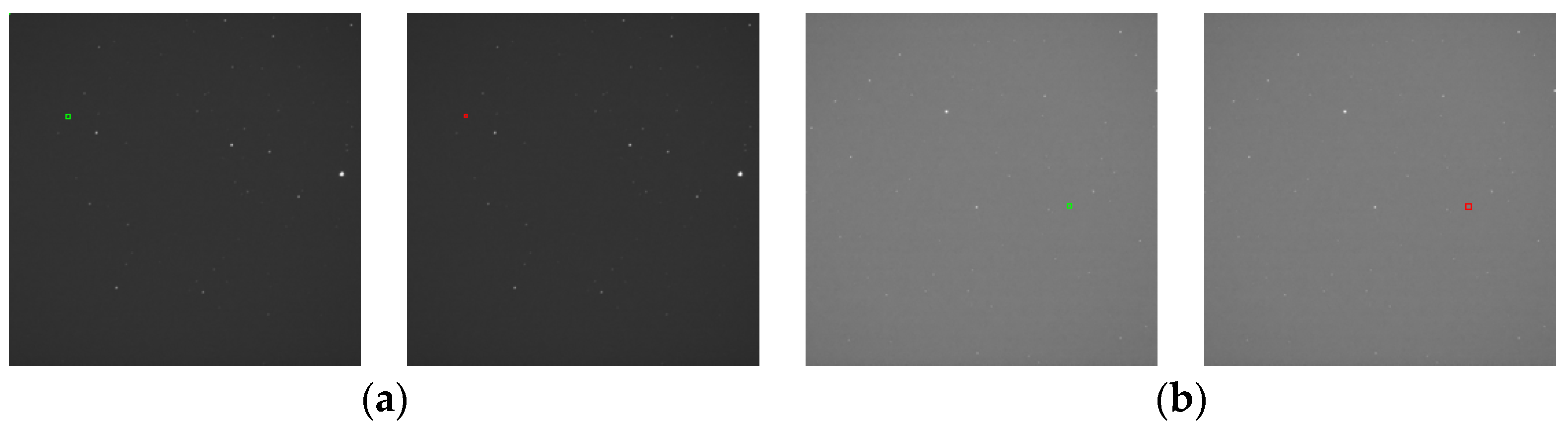
Figure 2.
Schematic diagram of point-like and streak-like targets in a star image in sidereal tracking mode: (a) point-like target (marked by a square) and (b) streak-like target (marked by an arrow).
Figure 2.
Schematic diagram of point-like and streak-like targets in a star image in sidereal tracking mode: (a) point-like target (marked by a square) and (b) streak-like target (marked by an arrow).
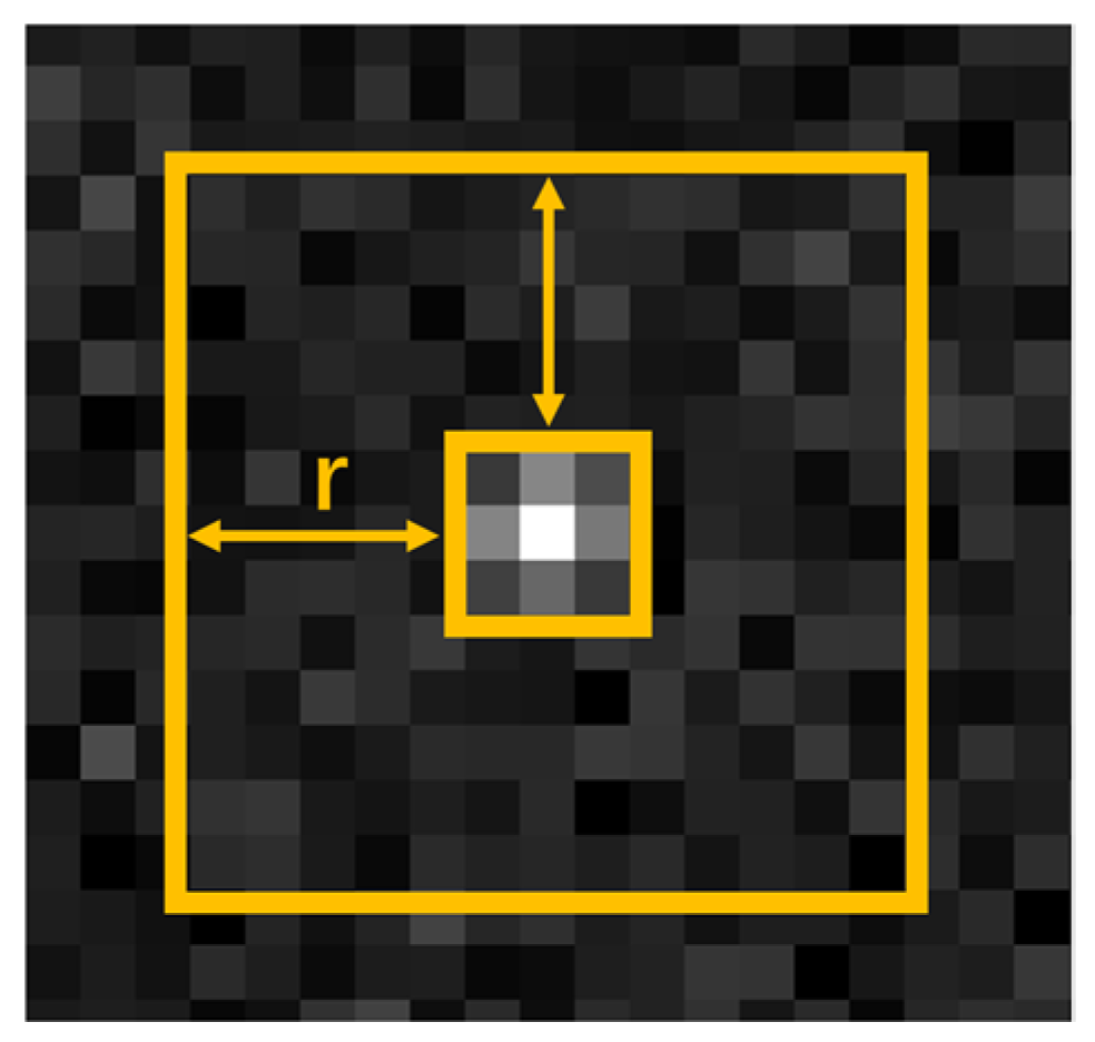
Figure 3.
Schematic representation showing the calculation of the target SNR.
Figure 3.
Schematic representation showing the calculation of the target SNR.
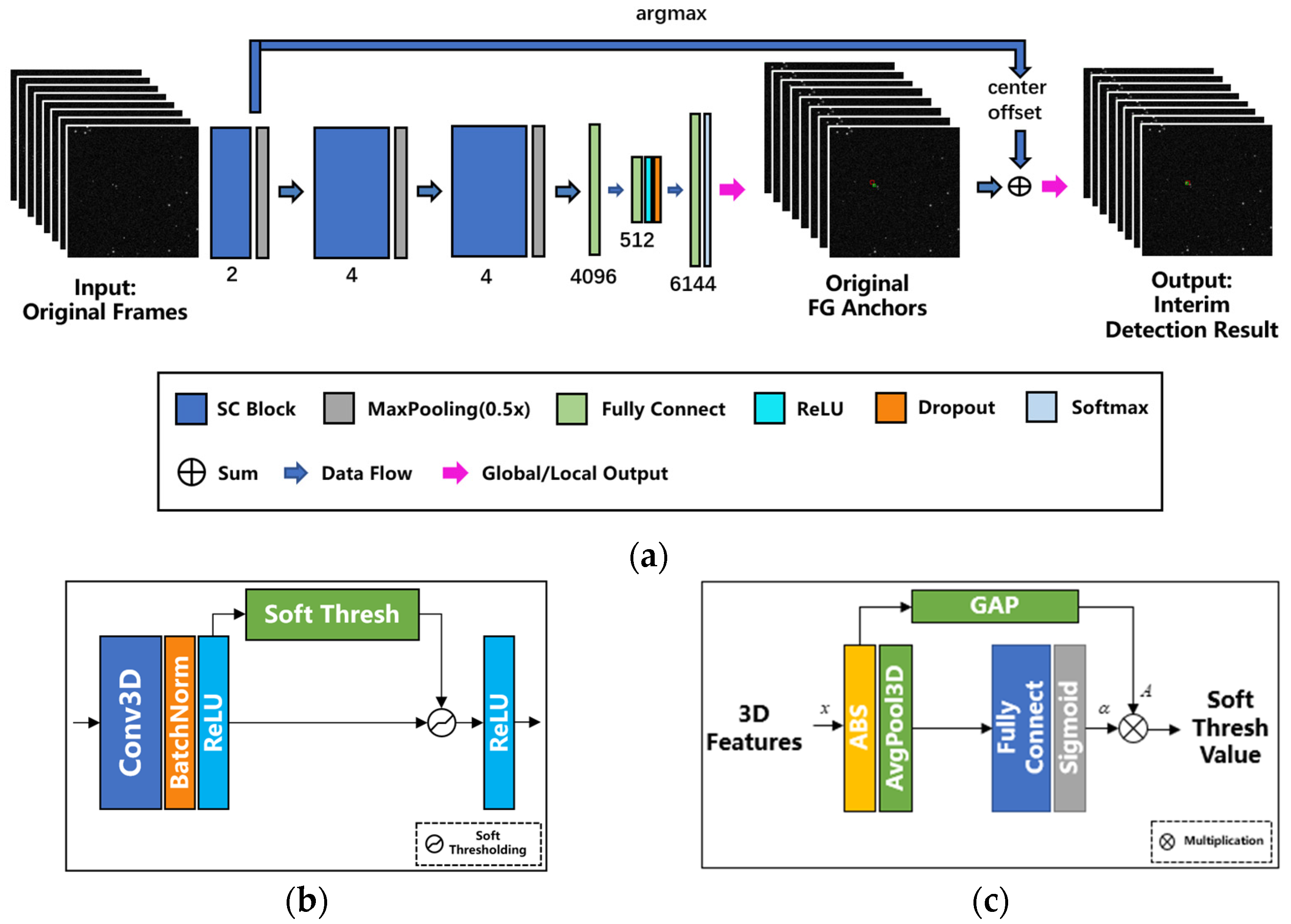
Figure 4.
(a) Architecture of the proposed detection network, (b) the internal architecture of an SC Block, and (c) the internal architecture of a soft thresholding module.
Figure 4.
(a) Architecture of the proposed detection network, (b) the internal architecture of an SC Block, and (c) the internal architecture of a soft thresholding module.
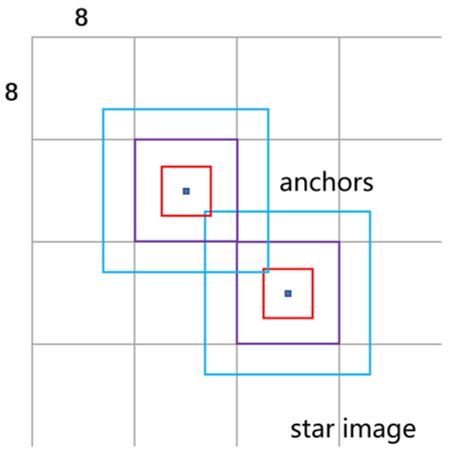
Figure 5.
Diagram of the anchors placed on the star image. The sizes of the blue, purple, and red anchors in the figure are 16 16, 8 8, and 4 4, respectively, with dots representing the center of the grid.
Figure 5.
Diagram of the anchors placed on the star image. The sizes of the blue, purple, and red anchors in the figure are 16 16, 8 8, and 4 4, respectively, with dots representing the center of the grid.
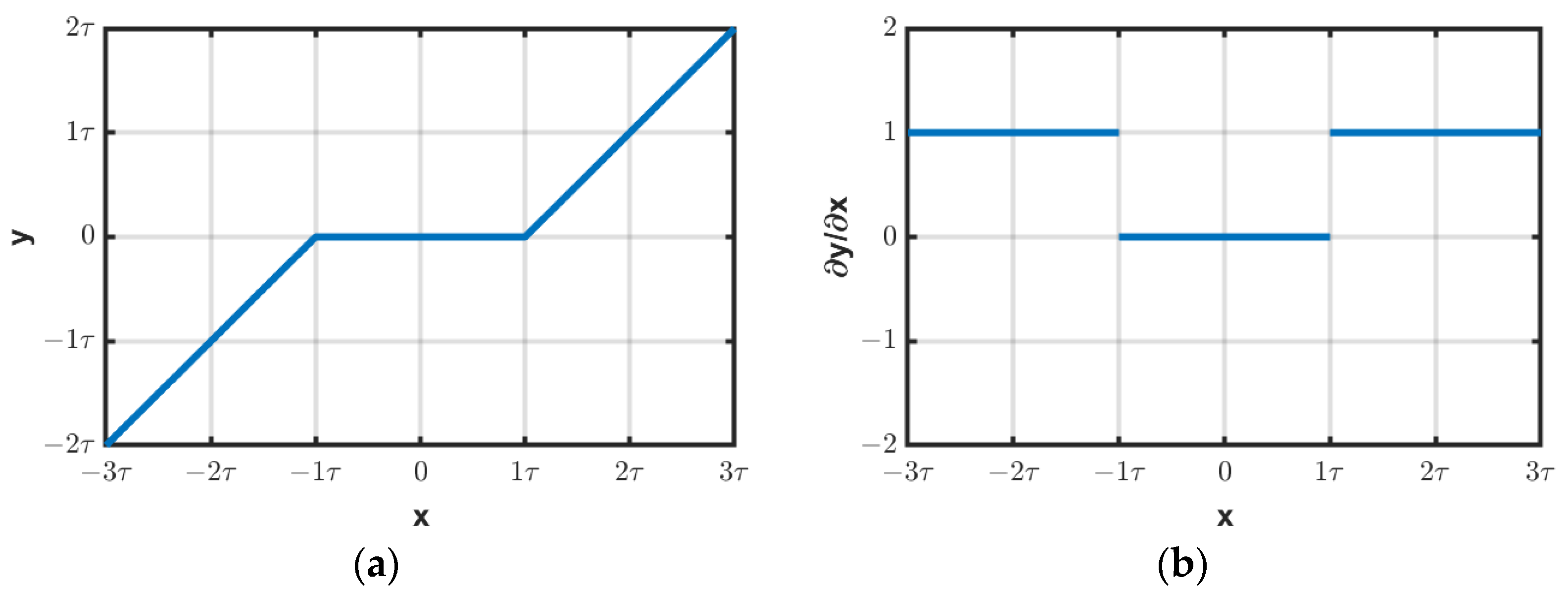
Figure 6.
(a) Relationship between the input and output of soft thresholding and its (b) derivative.
Figure 6.
(a) Relationship between the input and output of soft thresholding and its (b) derivative.
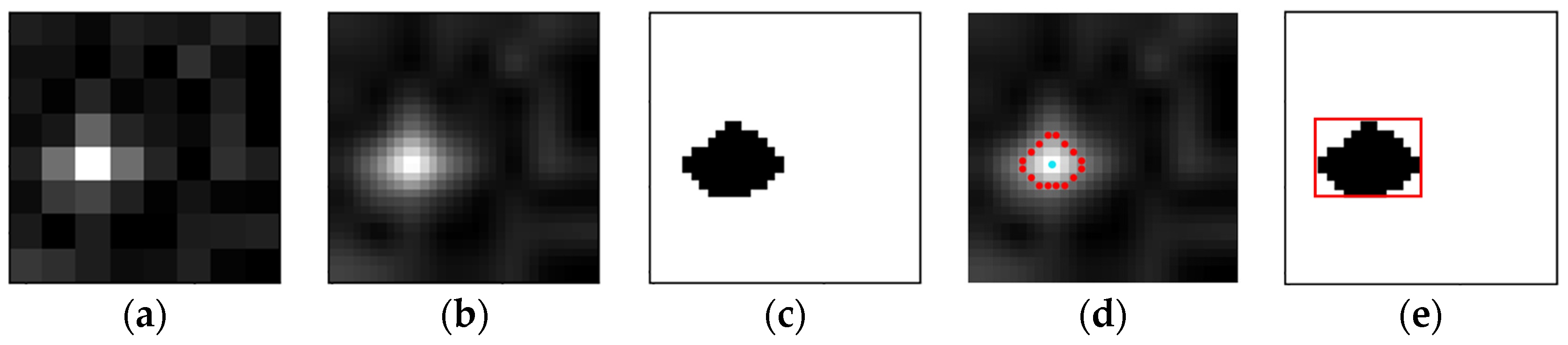
Figure 7.
(a) Original image within the positive anchor; (b) image after bilinear interpolation; (c) results of target/background segmentation after k-means clustering; (d) the red dots represent the pixels whose grayscale value is closest to the cluster center of the target region, and the blue dot represents the center derived by averaging the coordinates of the pixels; and (e) the window of the target region (the red rectangle) obtained by calculating the outer rectangle of the outer contour of the target region.
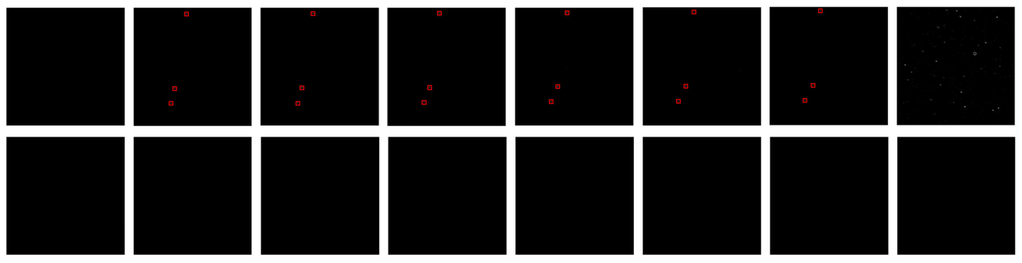
Figure 8.
Examples of the positional relationship between the positive anchor output by the detection network (the red anchors) and the ground truth of the target (the green boxes).
Figure 8.
Examples of the positional relationship between the positive anchor output by the detection network (the red anchors) and the ground truth of the target (the green boxes).
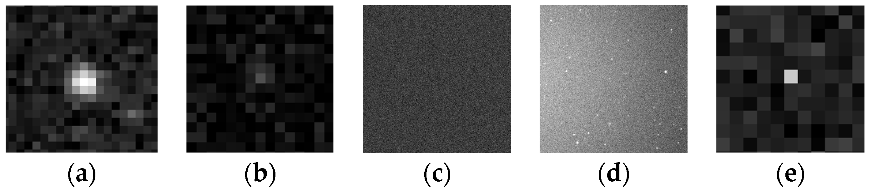
Figure 9.
Simulation results for typical elements of the image: (a) bright star; (b) dim target; (c); noise; (d) background; and (e) hot-pixel.
Figure 9.
Simulation results for typical elements of the image: (a) bright star; (b) dim target; (c); noise; (d) background; and (e) hot-pixel.
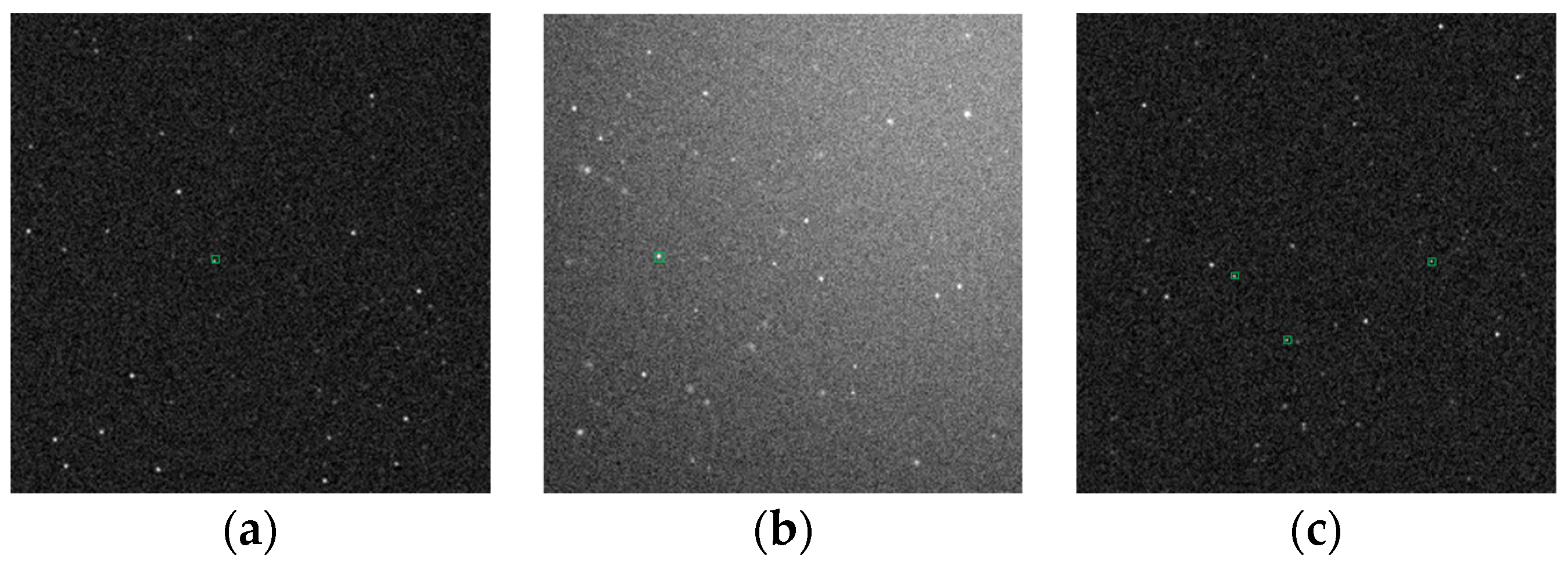
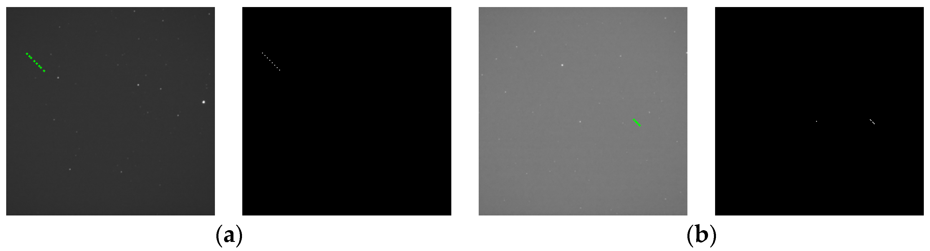
Figure 10.
Examples of simulated images: (a) a target and a background containing no stray light; (b) a target and a background containing stray light; and (c) three targets and a background containing no stray light. The targets are marked with green boxes.
Figure 10.
Examples of simulated images: (a) a target and a background containing no stray light; (b) a target and a background containing stray light; and (c) three targets and a background containing no stray light. The targets are marked with green boxes.
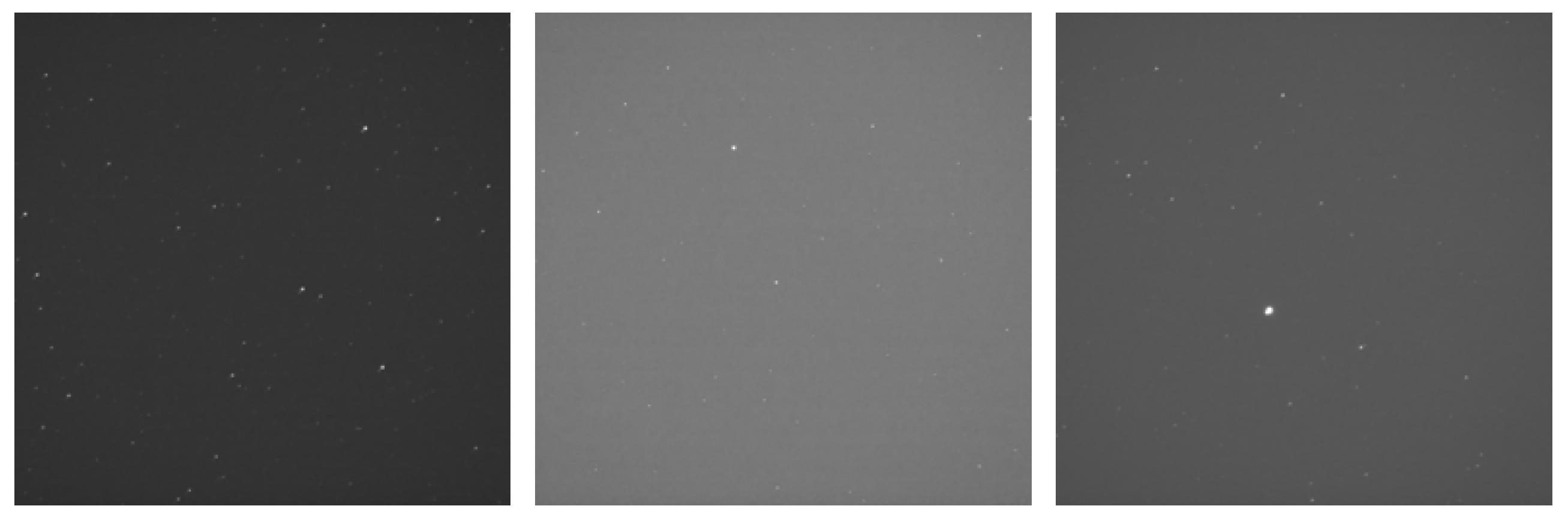
Figure 11.
Examples of real star images.
Figure 11.
Examples of real star images.
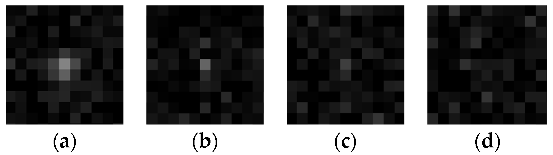
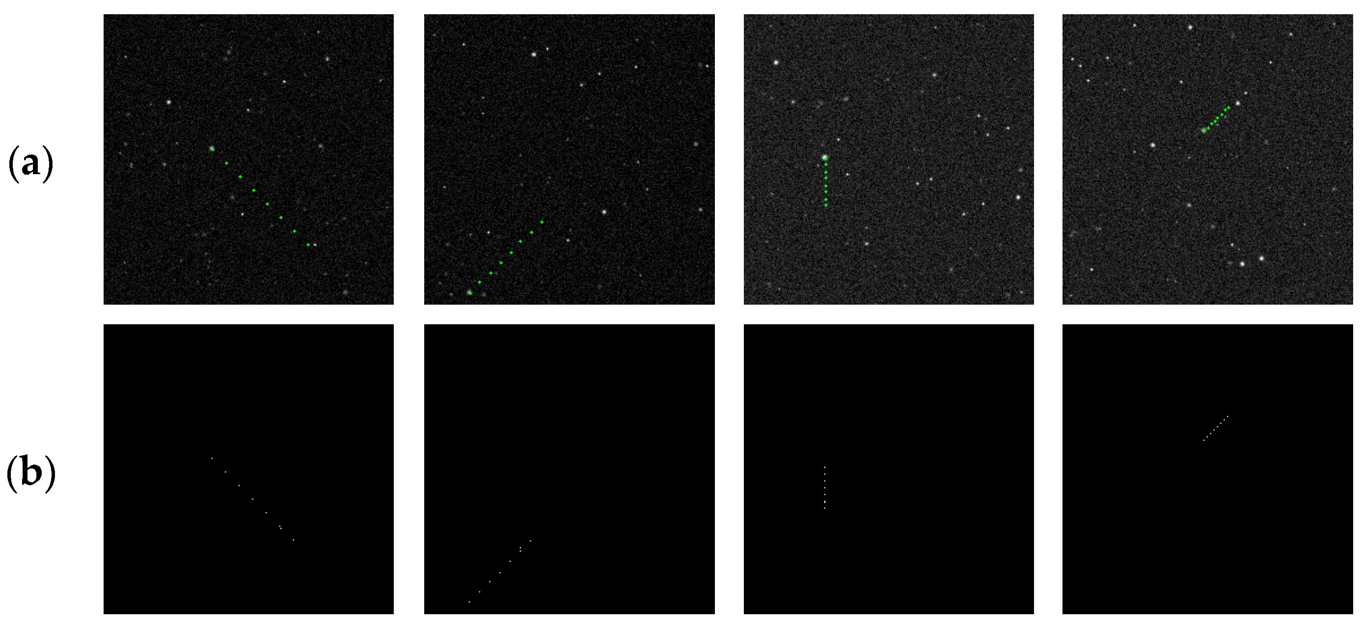
Figure 12.
Examples of simulated targets with different SNRs. (a) SNR = 3; (b) SNR = 1.5; (c) SNR = 1; and (d) SNR = 0.7.
Figure 12.
Examples of simulated targets with different SNRs. (a) SNR = 3; (b) SNR = 1.5; (c) SNR = 1; and (d) SNR = 0.7.
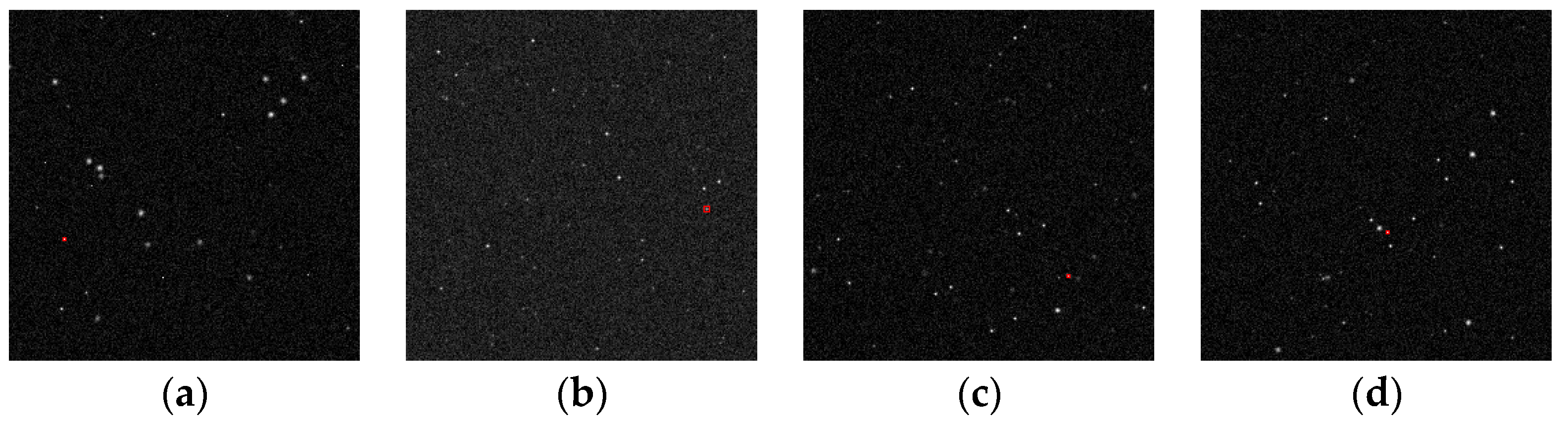
Figure 13.
Detection results on the first frame of four image sequences containing targets with different SNRs. (a) SNR = 3; (b) SNR = 1.5 (c) SNR = 1; and (d) SNR = 0.7. The targets were enclosed by the red bounding box output using our algorithm.
Figure 13.
Detection results on the first frame of four image sequences containing targets with different SNRs. (a) SNR = 3; (b) SNR = 1.5 (c) SNR = 1; and (d) SNR = 0.7. The targets were enclosed by the red bounding box output using our algorithm.
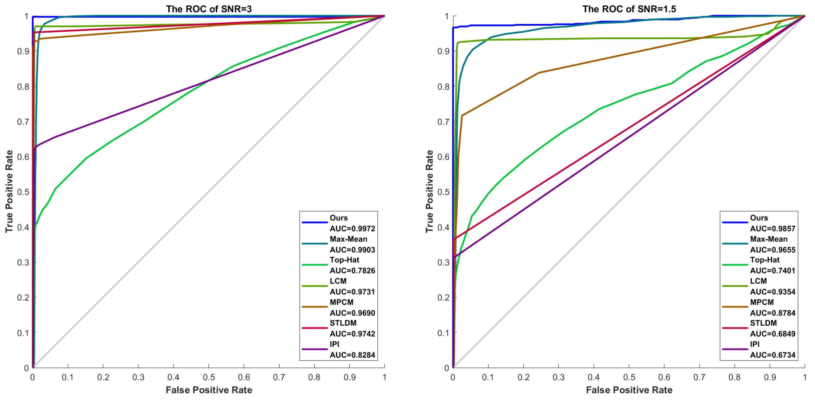
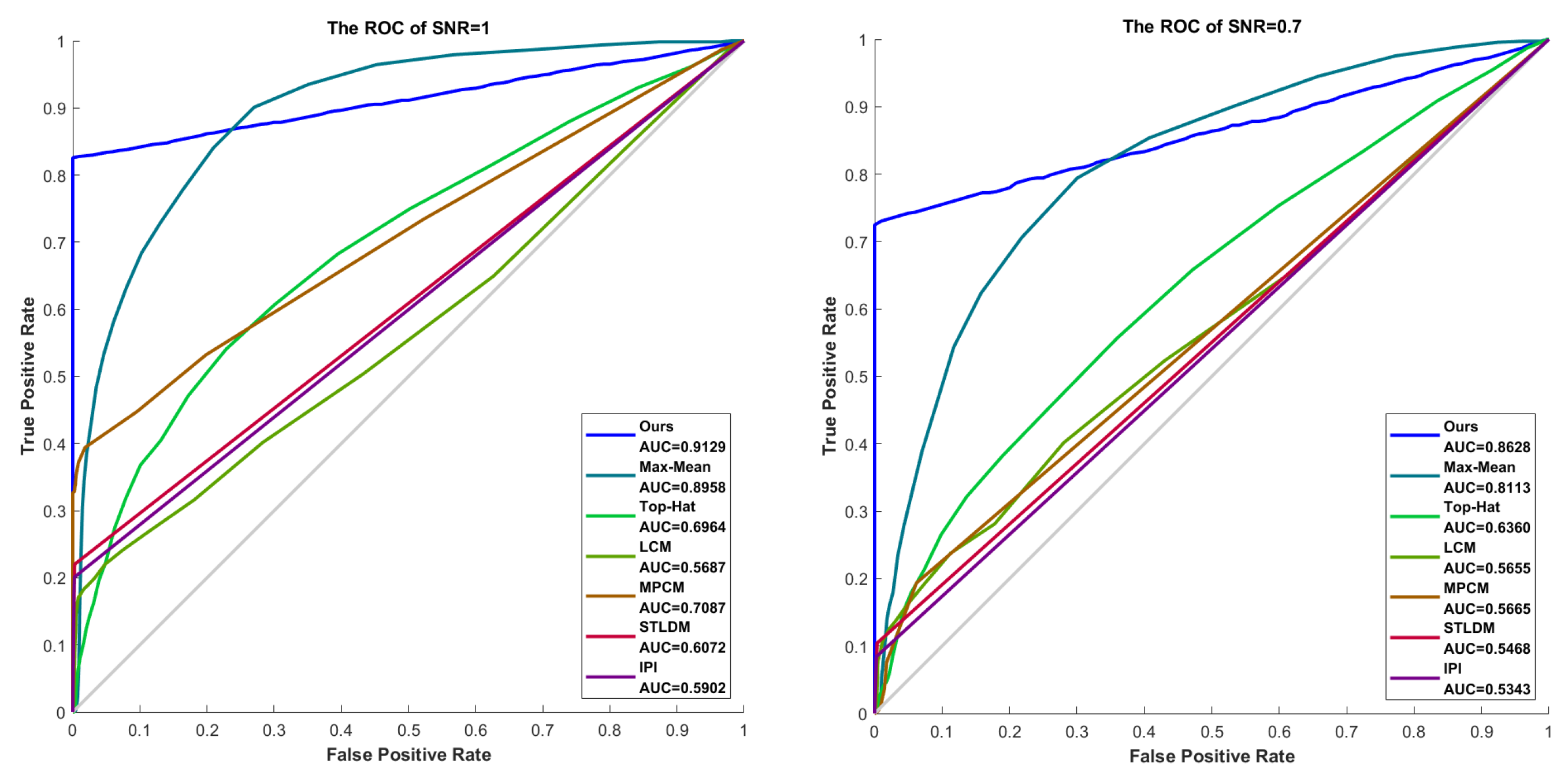
Figure 14.
The ROC curves for different SNRs.
Figure 14.
The ROC curves for different SNRs.
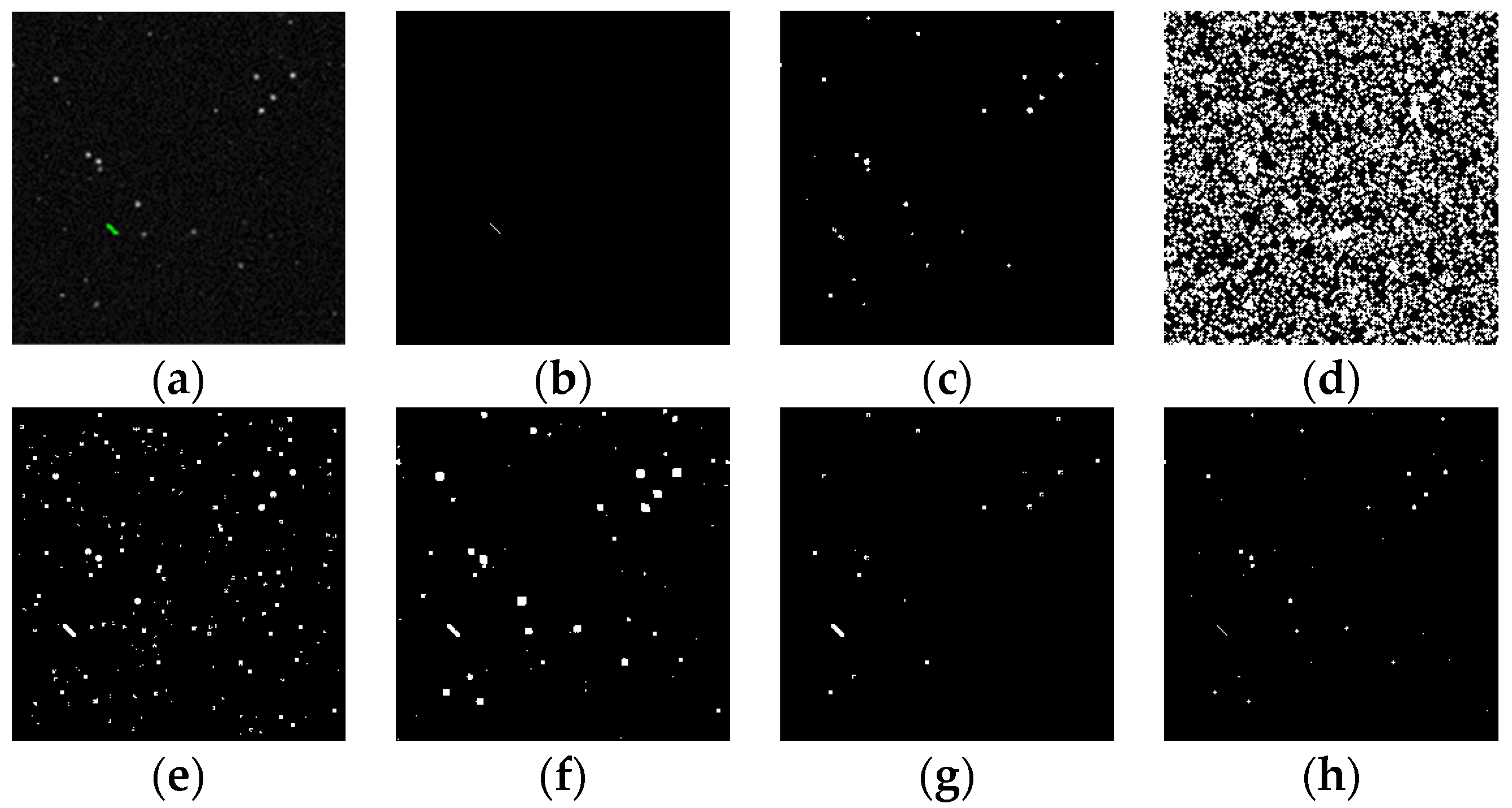
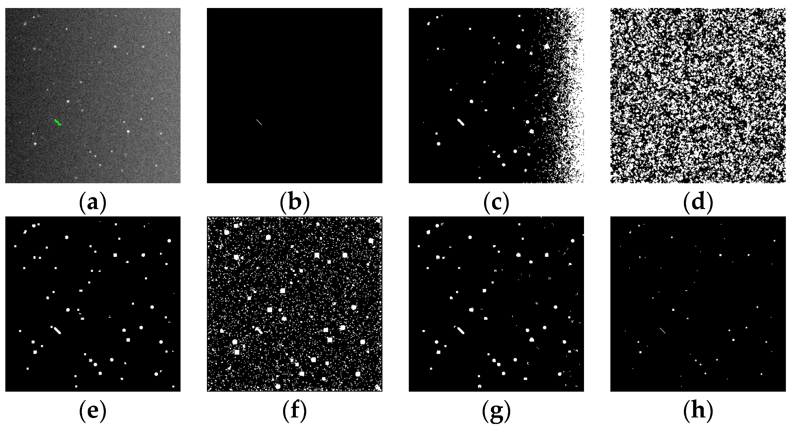
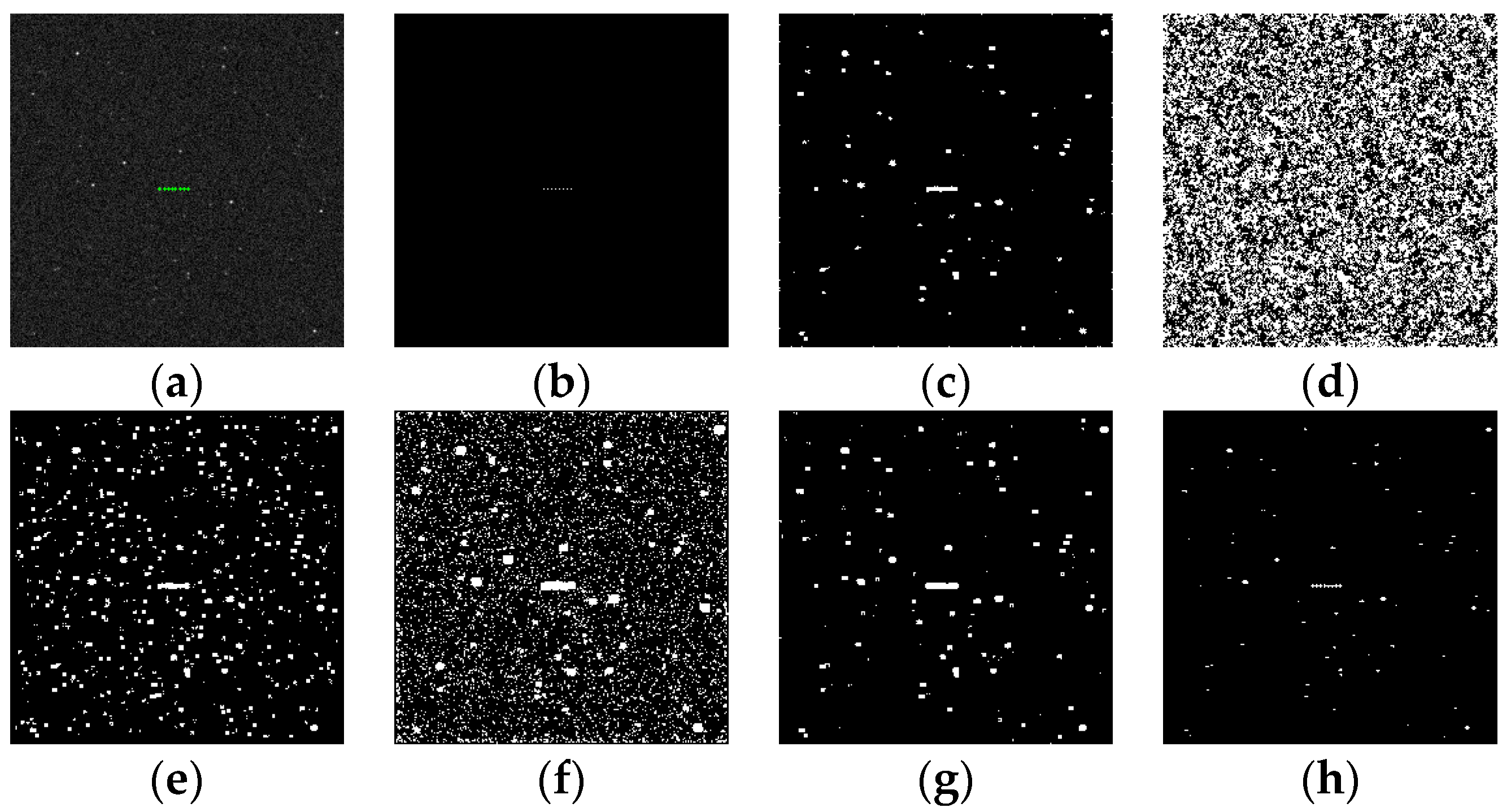
Figure 15.
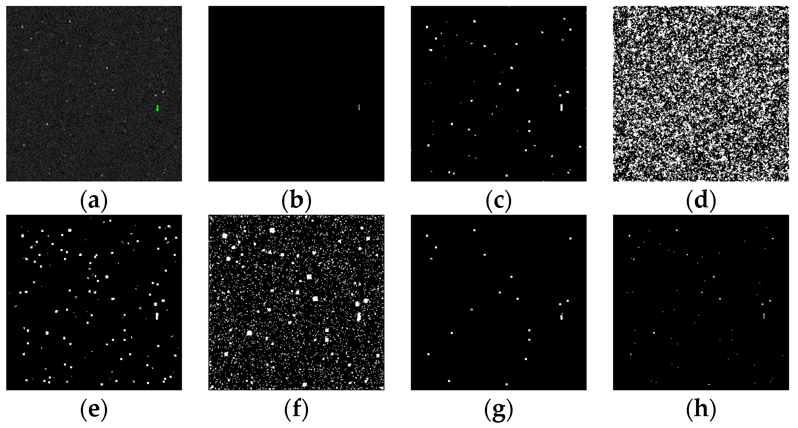
Detection results of target SNR = 3: (a) ground truth; (b) ours; (c) Max–Mean; (d) Top-Hat; (e) LCM; (f) MPCM; (g) STLDM; and (h) IPI.
Figure 15.
Detection results of target SNR = 3: (a) ground truth; (b) ours; (c) Max–Mean; (d) Top-Hat; (e) LCM; (f) MPCM; (g) STLDM; and (h) IPI.
Figure 16.
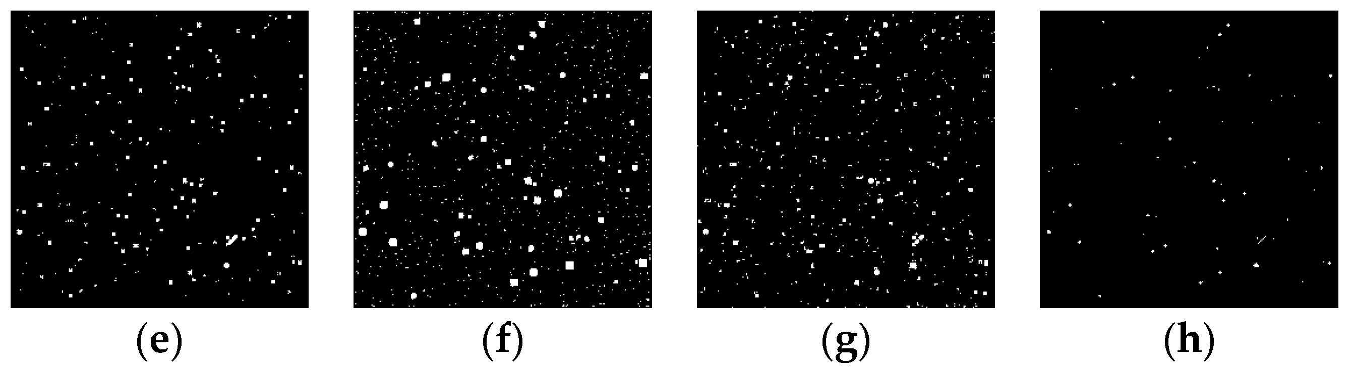
Detection results of target SNR = 1.5: (a) ground truth; (b) ours; (c) Max–Mean; (d) Top-Hat; (e) LCM; (f) MPCM; (g) STLDM; and (h) IPI.
Figure 16.
Detection results of target SNR = 1.5: (a) ground truth; (b) ours; (c) Max–Mean; (d) Top-Hat; (e) LCM; (f) MPCM; (g) STLDM; and (h) IPI.
Figure 17.
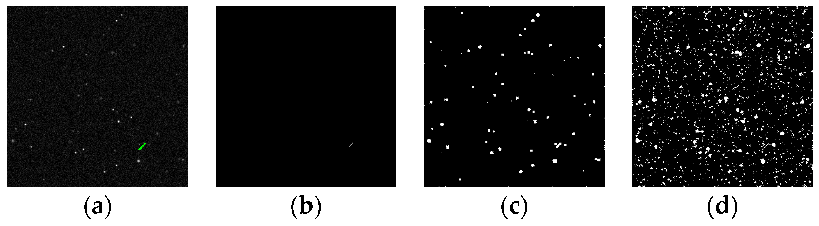
Detection results of target SNR = 1: (a) ground truth; (b) ours; (c) Max–Mean; (d) Top-Hat; (e) LCM; (f) MPCM; (g) STLDM; and (h) IPI.
Figure 17.
Detection results of target SNR = 1: (a) ground truth; (b) ours; (c) Max–Mean; (d) Top-Hat; (e) LCM; (f) MPCM; (g) STLDM; and (h) IPI.
Figure 18.
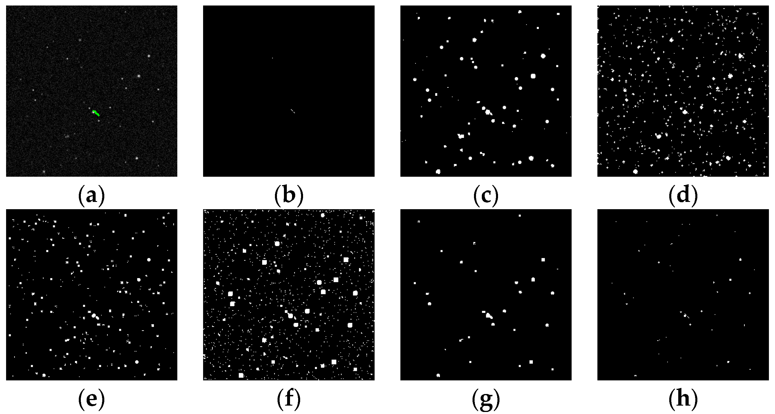
Detection results of target SNR = 0.7: (a) ground truth; (b) ours; (c) Max–Mean; (d) Top-Hat; (e) LCM; (f) MPCM; (g) STLDM; and (h) IPI.
Figure 18.
Detection results of target SNR = 0.7: (a) ground truth; (b) ours; (c) Max–Mean; (d) Top-Hat; (e) LCM; (f) MPCM; (g) STLDM; and (h) IPI.
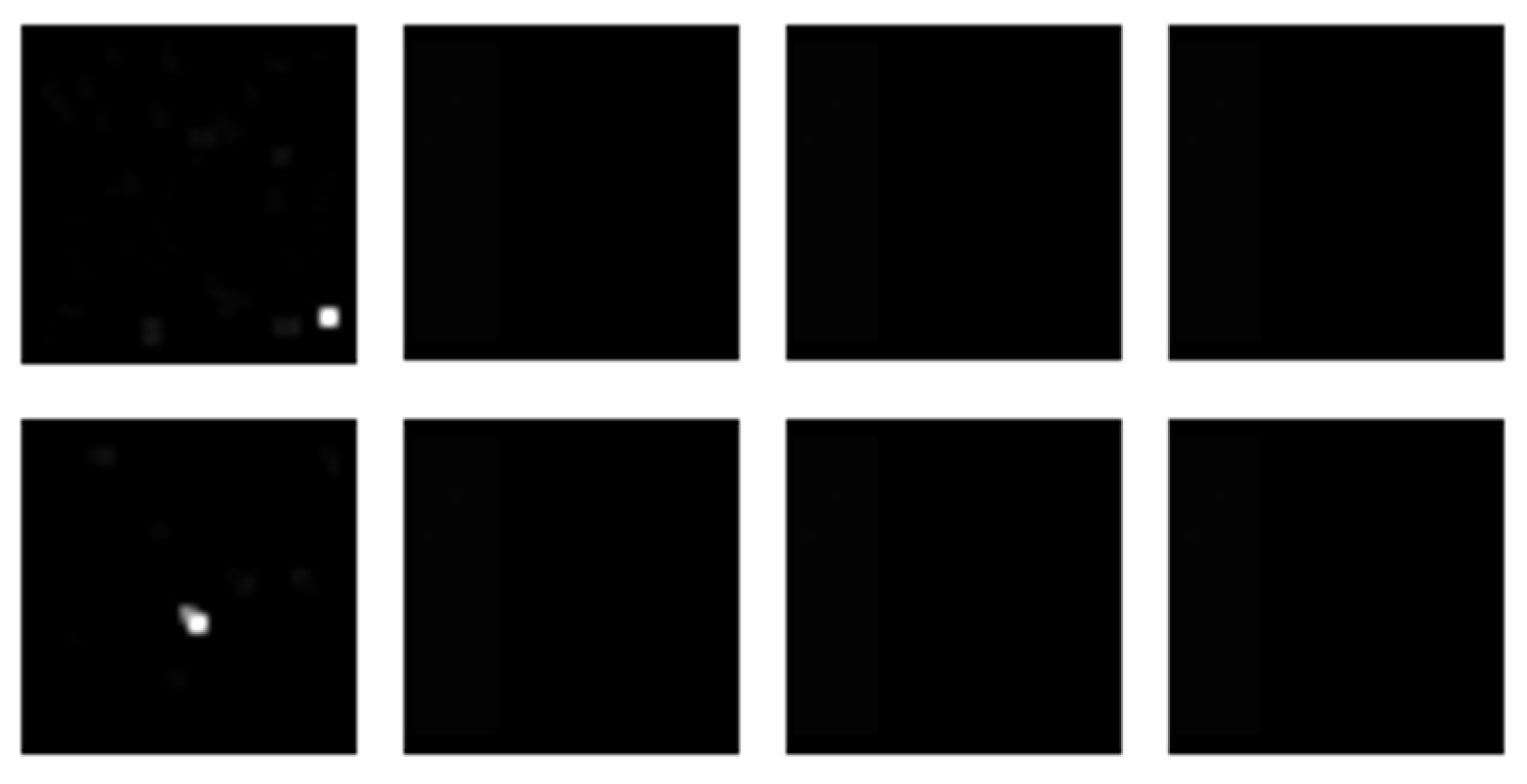
Figure 19.
Each row is an example of the final feature maps when SNR = 1 and SNR = 0.7, respectively. Each of them has a size of 4 1 32 32 (4 channels with 1 frame of size 32 32 for each channel).
Figure 19.
Each row is an example of the final feature maps when SNR = 1 and SNR = 0.7, respectively. Each of them has a size of 4 1 32 32 (4 channels with 1 frame of size 32 32 for each channel).
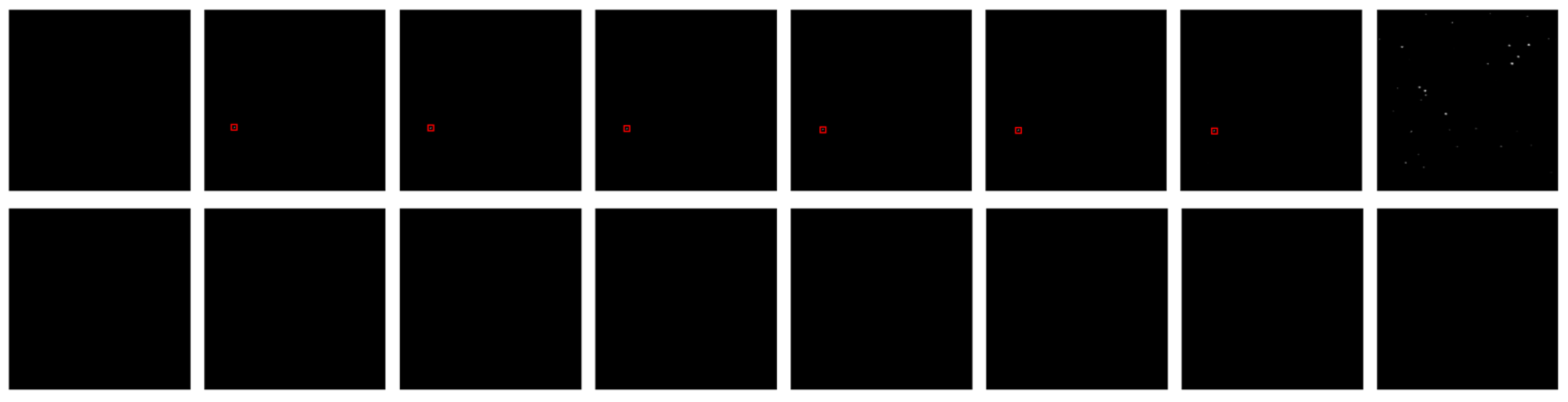
Figure 20.
Example of the feature maps output by the 1st SC Block when SNR = 3, with a size of 2 8 256 256 (2 channels with 8 frames of size 256 256). The red boxes indicates the feature response of the target.
Figure 20.
Example of the feature maps output by the 1st SC Block when SNR = 3, with a size of 2 8 256 256 (2 channels with 8 frames of size 256 256). The red boxes indicates the feature response of the target.
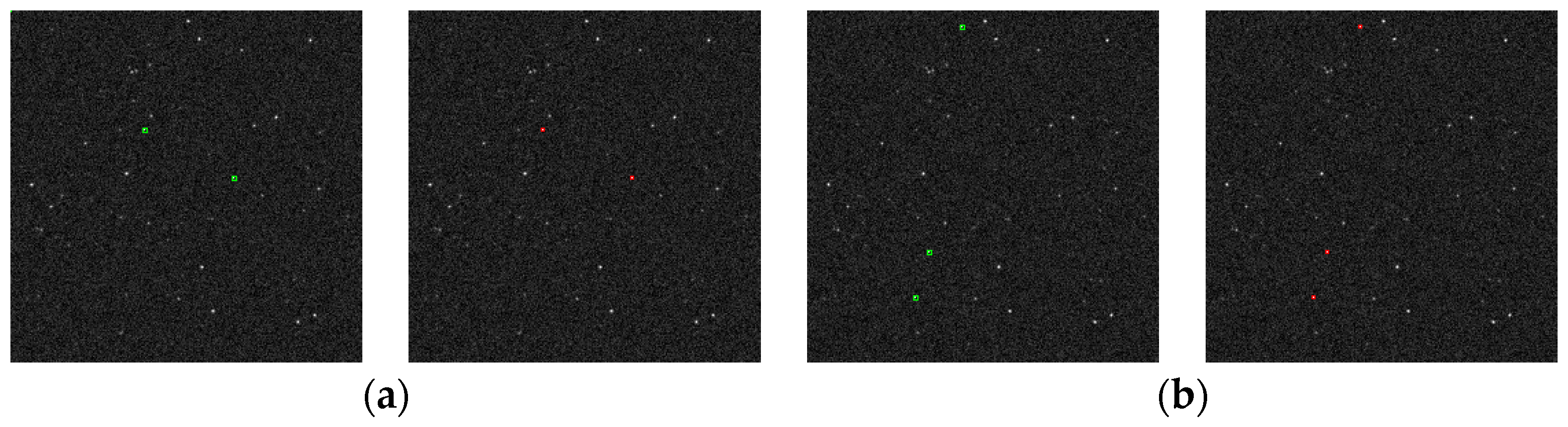
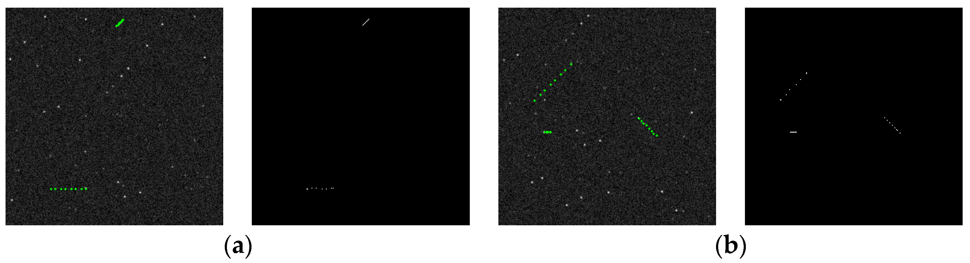
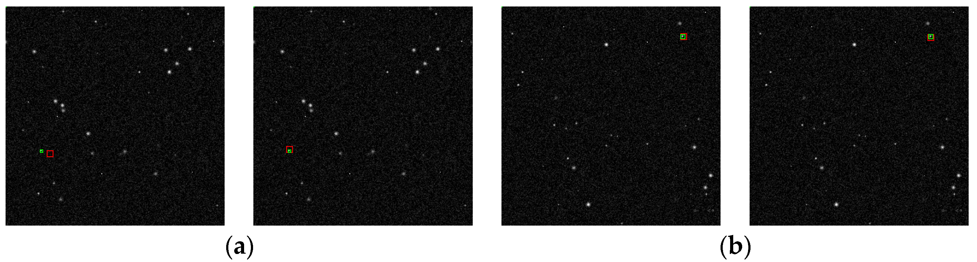
Figure 21.
Example of the detection results on the first frame of two image sequences. (a) contains two targets and (b) contains three targets. In each pair, the left is the ground truth of the target, and the right is the detection result.
Figure 21.
Example of the detection results on the first frame of two image sequences. (a) contains two targets and (b) contains three targets. In each pair, the left is the ground truth of the target, and the right is the detection result.
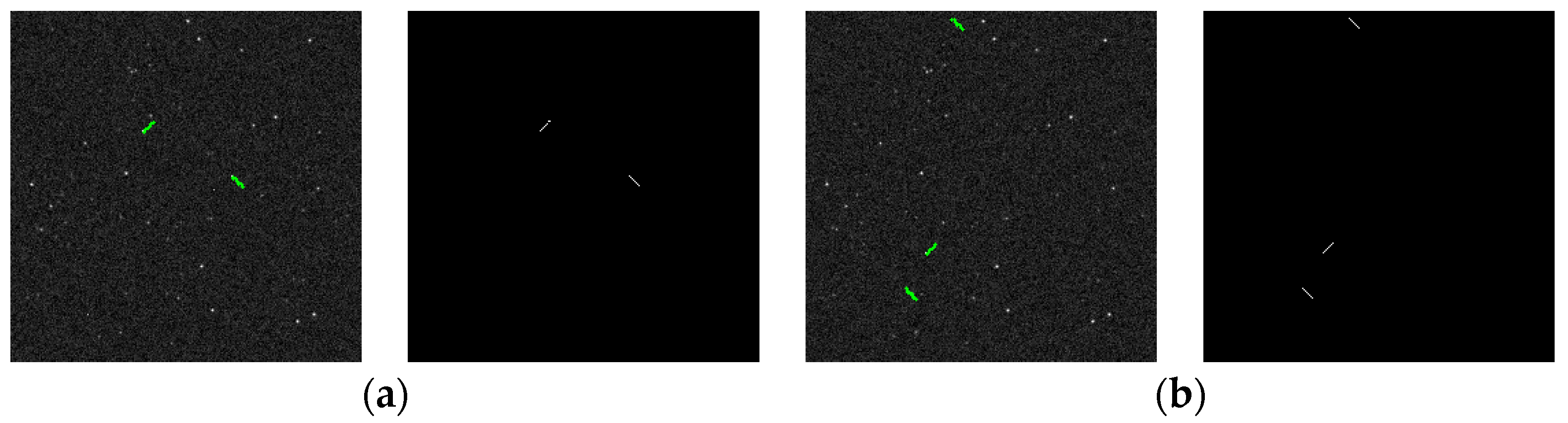
Figure 22.
Example of a target trajectory output by the proposed method for two image sequences. (a) contains two targets and (b) contains three targets. In each pair, the left is the ground truth of the target, and the right is the detection result.
Figure 22.
Example of a target trajectory output by the proposed method for two image sequences. (a) contains two targets and (b) contains three targets. In each pair, the left is the ground truth of the target, and the right is the detection result.
Figure 23.
Example of the feature maps output by the 1st SC Block when target number = 3, with a size of 2 8 256 256 (2 channels with 8 frames of size 256 256). The red boxes indicates the feature response of the target.
Figure 23.
Example of the feature maps output by the 1st SC Block when target number = 3, with a size of 2 8 256 256 (2 channels with 8 frames of size 256 256). The red boxes indicates the feature response of the target.
Figure 24.
Example of target trajectories of different speeds. From left to right: speed = 12, speed = 9, speed = 6, and speed = 3. The first row (a): ground truths; the second row (b): results.
Figure 24.
Example of target trajectories of different speeds. From left to right: speed = 12, speed = 9, speed = 6, and speed = 3. The first row (a): ground truths; the second row (b): results.
Figure 25.
Example of a target trajectory output by the proposed method for two image sequences containing two and three targets with different speeds in the same sequence: (a) speed = 6 and 1; (b) speed = 6, 3, and 1. In each pair, the left is the ground truth of the target, and the right is the detection result.
Figure 26.
Detection results of image sequences with stray light: (a) ground truth; (b) ours; (c) Max–Mean; (d) Top-Hat; (e) LCM; (f) MPCM; (g) STLDM; and (h) IPI.
Figure 26.
Detection results of image sequences with stray light: (a) ground truth; (b) ours; (c) Max–Mean; (d) Top-Hat; (e) LCM; (f) MPCM; (g) STLDM; and (h) IPI.
Figure 27.
Detection results of image sequences with slowly moving backgrounds: (a) ground truth; (b) ours; (c) Max–Mean; (d) Top-Hat; (e) LCM; (f) MPCM; (g) STLDM; and (h) IPI.
Figure 27.
Detection results of image sequences with slowly moving backgrounds: (a) ground truth; (b) ours; (c) Max–Mean; (d) Top-Hat; (e) LCM; (f) MPCM; (g) STLDM; and (h) IPI.
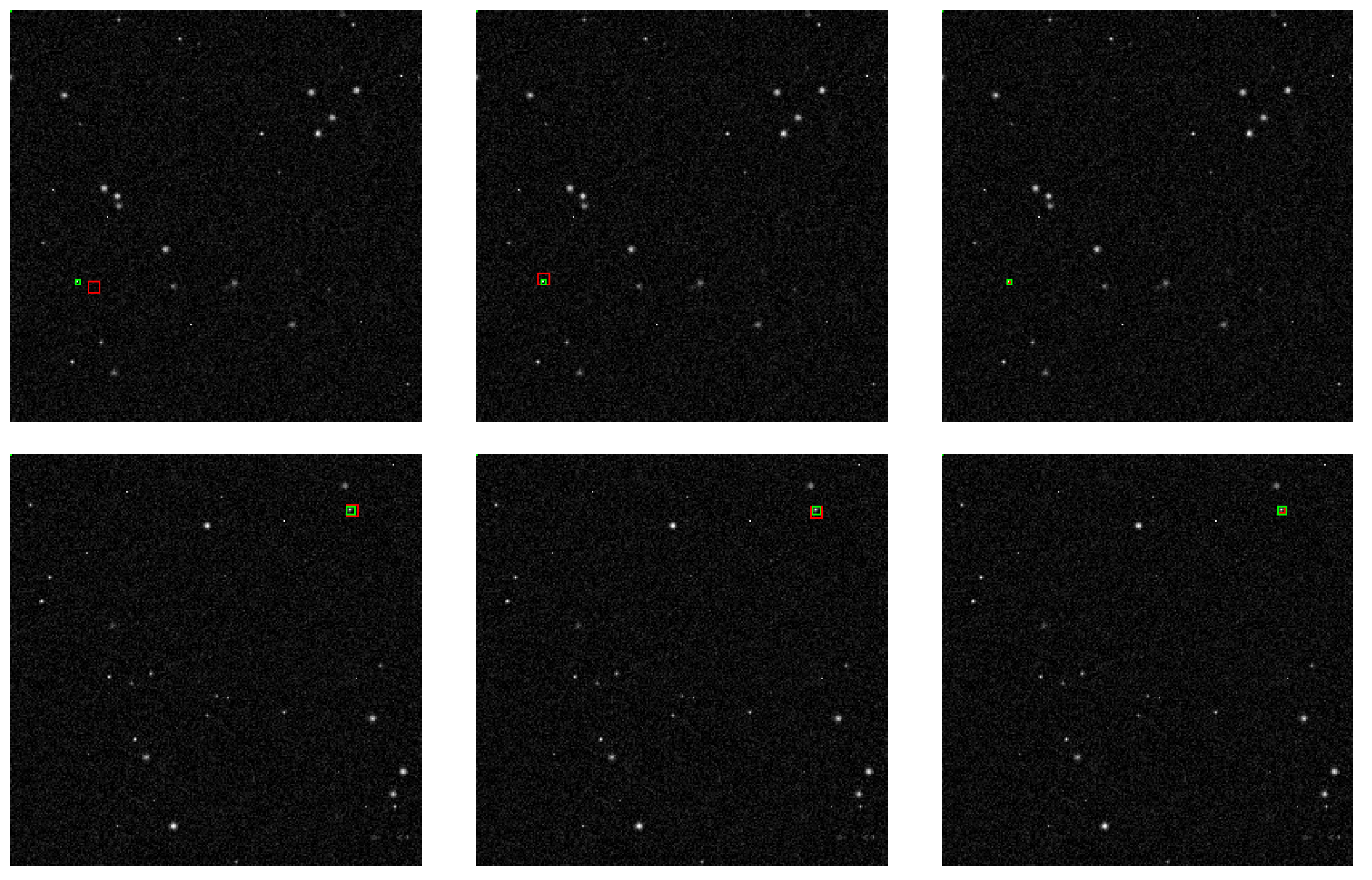
Figure 28.
Two examples of the effect of branch offsetting the original anchors (pair (a,b)). The green boxes are the ground truth, and the red boxes are anchors. In each pair, the left is the original anchor and the right is the result after the branch offset.
Figure 28.
Two examples of the effect of branch offsetting the original anchors (pair (a,b)). The green boxes are the ground truth, and the red boxes are anchors. In each pair, the left is the original anchor and the right is the result after the branch offset.
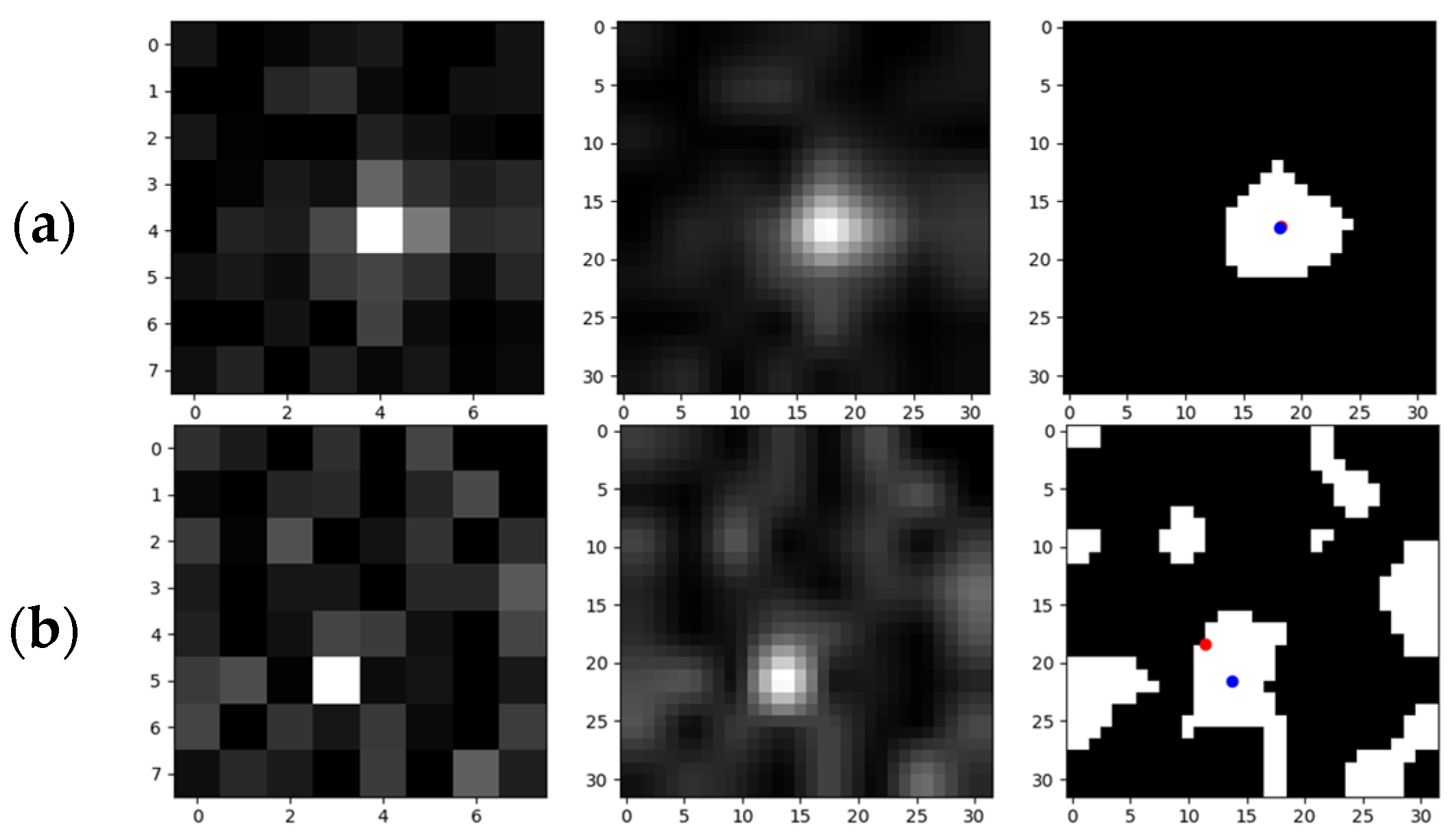
Figure 29.
Examples of the validity of centroid iterations: (a) the 1st row: a target with higher SNR, and the effect of the precision enhancement of the iteration is not obvious; (b) the 2nd row: a target with lower SNR (stronger background noise), and the effect of precision enhancement of the iteration is obvious. The red dot and the blue dot represents the pre and post-iteration centroid positions, respectively.
Figure 30.
Examples of the effect of the overall positioning process in this study. The third column reflects the changes after processing via the k-means centroid positioning method. The green boxes are ground truth, and the red boxes are anchors.
Figure 30.
Examples of the effect of the overall positioning process in this study. The third column reflects the changes after processing via the k-means centroid positioning method. The green boxes are ground truth, and the red boxes are anchors.
Figure 31.
An example of the detection results for the first frame of two image sequences containing targets with (a) SNR = 3, speed = 3 and (b) SNR = 0.7, speed = 1. In each pair, the left is the ground truth of the target, and the right is the detection result.
Figure 31.
An example of the detection results for the first frame of two image sequences containing targets with (a) SNR = 3, speed = 3 and (b) SNR = 0.7, speed = 1. In each pair, the left is the ground truth of the target, and the right is the detection result.
Figure 32.
An example of a target trajectory output by the proposed method of two image sequences containing targets with (a) SNR = 3, speed = 3 and (b) SNR = 0.7, speed = 1. In each pair, the left is the ground truth of the target, and the right is the detection result.
Figure 32.
An example of a target trajectory output by the proposed method of two image sequences containing targets with (a) SNR = 3, speed = 3 and (b) SNR = 0.7, speed = 1. In each pair, the left is the ground truth of the target, and the right is the detection result.
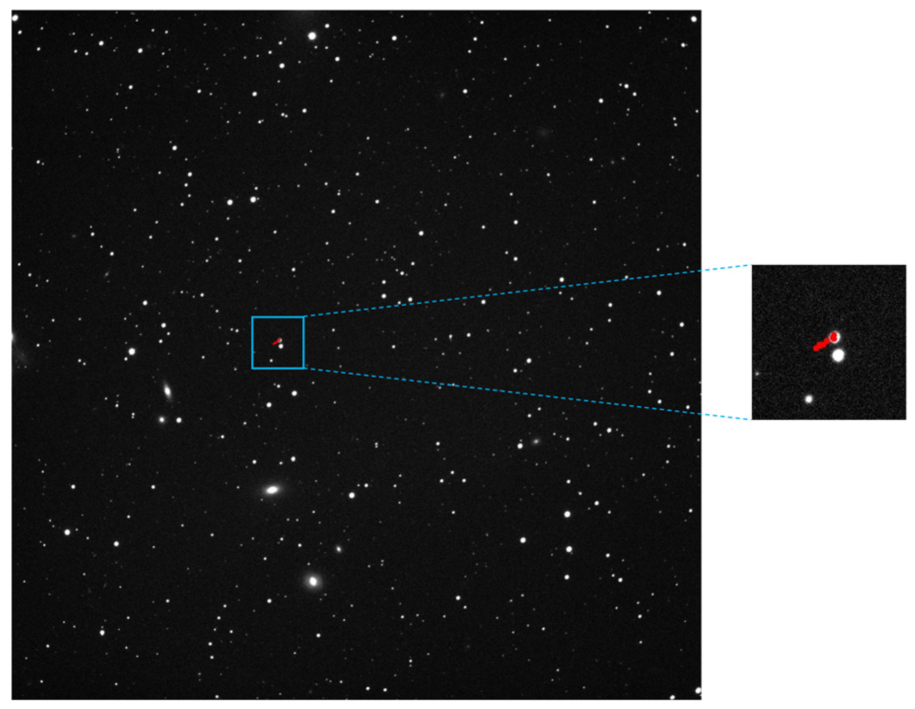
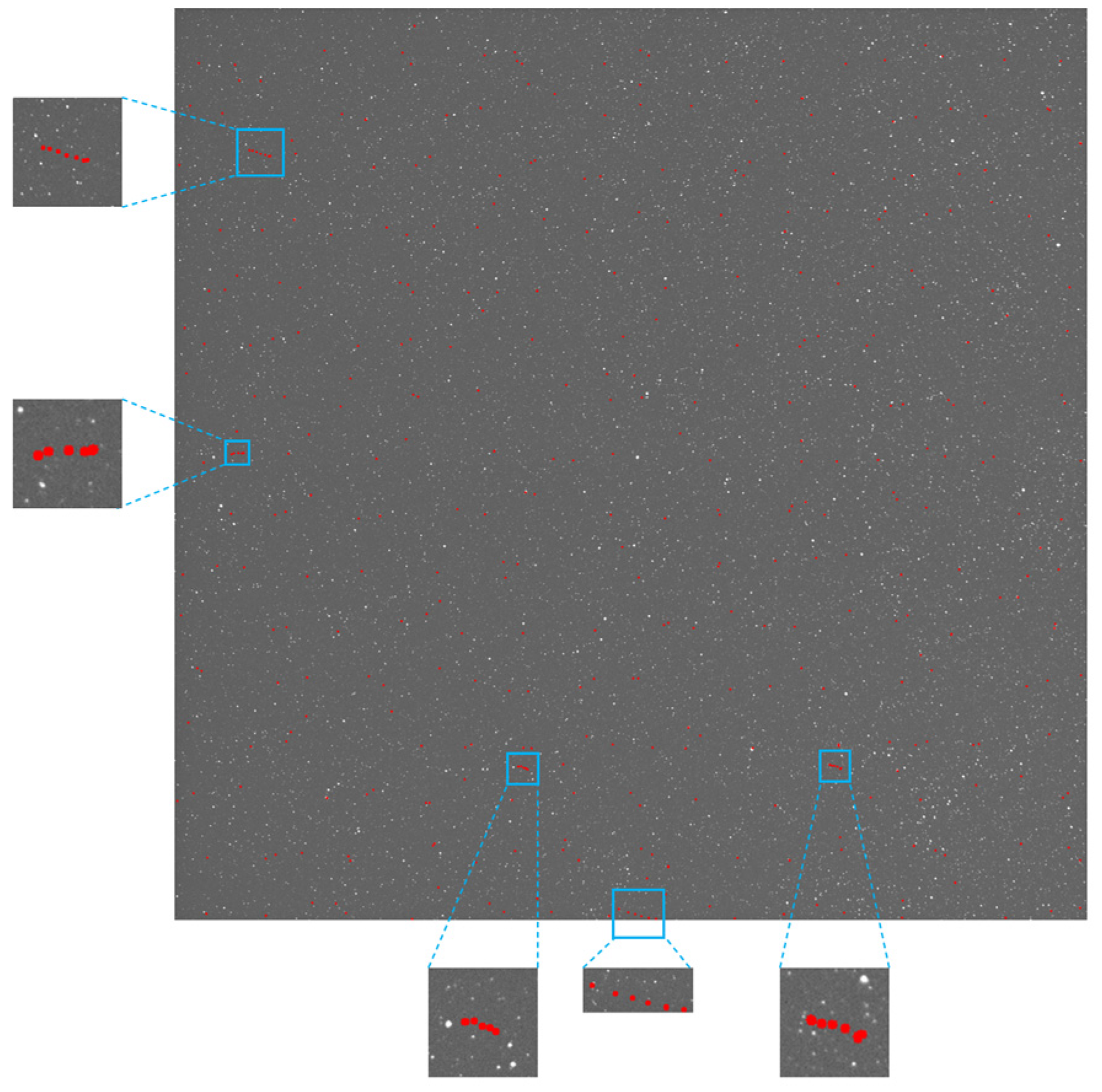
Figure 33.
The target detection results of asteroid 194 via the proposed method; the trajectory area has been enlarged for display, with the trajectory marked by a red dotted line.
Figure 33.
The target detection results of asteroid 194 via the proposed method; the trajectory area has been enlarged for display, with the trajectory marked by a red dotted line.
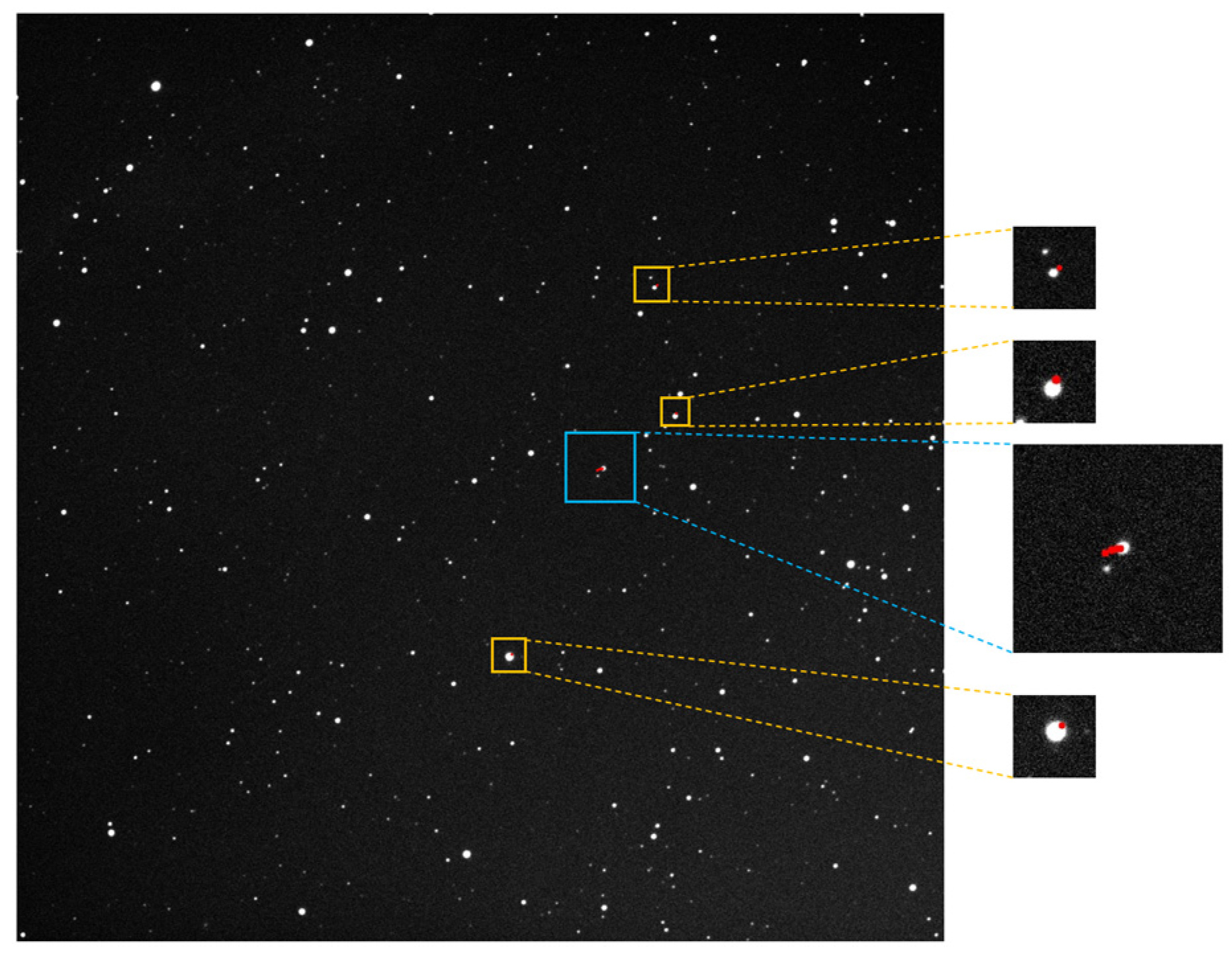
Figure 34.
The target detection results of asteroid 145 via the proposed method; the trajectory area has been enlarged for display, with the correct trajectory marked in blue boxes and false detection points marked in yellow boxes with a red dotted line.
Figure 34.
The target detection results of asteroid 145 via the proposed method; the trajectory area has been enlarged for display, with the correct trajectory marked in blue boxes and false detection points marked in yellow boxes with a red dotted line.
Figure 35.
The target detection results via the proposed method; the trajectory area has been enlarged for display, with the trajectory marked in blue boxes with a red dotted line.
Figure 35.
The target detection results via the proposed method; the trajectory area has been enlarged for display, with the trajectory marked in blue boxes with a red dotted line.
Table 1.
Hyperparameter settings for the architecture of the backbone network.
Table 1.
Hyperparameter settings for the architecture of the backbone network.
| Components of Backbone | Module Inside | Hyperparameters | Output Size
(C D H W) |
|---|
| Input | - | - | 1 8 256 256 |
| SC Block 1 | Conv 3D | kernel = (3 3 3) 2 | 2 8 256 256 |
| stride = 1 1 1 |
| padding = 1 1 1 |
| Soft Thresh | See Table 2 |
| Max Pool 3D 1 | - | kernel = 2 2 2 | 2 4 128 128 |
| stride = 1 1 1 |
| SC Block 2 | Conv 3D | kernel = (3 3 3) 4 | 4 4 128 128 |
| stride = 1 1 1 |
| padding = 1 1 1 |
| Soft Thresh | See Table 2 |
| Max Pool 3D 2 | - | kernel = 2 2 2 | 4 2 64 64 |
| stride = 1 1 1 |
| SC Block 3 | Conv 3D | kernel = (3 3 3) 4 | 4 2 64 64 |
| stride = 1 1 1 |
| padding = 1 1 1 |
| Soft Thresh | See Table 2 |
| Max Pool 3D 3 | - | kernel = 2 2 2 | 4 1 32 32 |
| stride = 1 1 1 |
| FC | FC Layers | layer = {4096, 512, 6144} | 4096 |
Table 2.
Hyperparameter settings for the structure of the soft thresholding module.
Table 2.
Hyperparameter settings for the structure of the soft thresholding module.
| Soft Thresh Module | Components | Hyperparameters | Output Size |
|---|
| In SC Block 1 | Input | - | 2 8 256 256 |
| GAP | 1 1 1 | 1 1 1 |
| Average Pool 3D | {kernel = 2 2 2, stride = 2 2 2} 3 | 2 1 32 32 |
| FC | layer = {2048, 256, 2} | 2 1 |
| Output | - | 2 1 |
| In SC Block 2 | Input | - | 4 4 128 128 |
| GAP | 1 1 1 | 1 1 1 |
| Average Pool 3D | {kernel = 2 2 2, stride = 2 2 2} 2 | 4 1 32 32 |
| FC | layer = {4096, 256, 4} | 4 1 |
| Output | - | 4 1 |
| In SC Block 3 | Input | - | 4 2 64 64 |
| GAP | 111 | 1 1 1 |
| Average Pool 3D | {kernel = 2 2 2, stride = 2 2 2} 1 | 4 1 32 32 |
| FC | layer = {4096, 256, 4} | 4 1 |
| Output | - | 4 1 |
Table 3.
Parameter settings for the experiments of detection performance of targets with different SNRs.
Table 3.
Parameter settings for the experiments of detection performance of targets with different SNRs.
| Target | Background |
|---|
| SNR | Number | Size | Speed | Stray Light | Slow Motion |
|---|
| 3, 1.5, 1, 0.7 | 1 | 7, 5, 3, 1 | 1 | No | No |
Table 4.
Detection performance results of targets with different SNRs.
Table 4.
Detection performance results of targets with different SNRs.
| SNRs | Metrics | Ours | Max–Mean | Top-Hat | LCM | MPCM | STLDM | IPI |
|---|
| 3 | Detection Rate (%) | 99.75 | 96.5 | 95.25 | 98.875 | 96.375 | 98.5 | 98.125 |
| False Alarm Rate (%) | 0.0243 | 0.5955 | 37.1474 | 1.2897 | 1.2183 | 0.2328 | 0.2074 |
| 1.5 | Detection Rate (%) | 96 | 96.375 | 96.625 | 93 | 97.25 | 95.75 | 93.875 |
| False Alarm Rate (%) | 0.0206 | 0.7234 | 39.0416 | 1.4999 | 8.7156 | 0.3196 | 0.2179 |
| 1 | Detection Rate (%) | 83 | 81.875 | 85.25 | 82.5 | 82.75 | 84.875 | 68.875 |
| False Alarm Rate (%) | 0.0260 | 0.8782 | 8.2603 | 1.6380 | 3.0551 | 2.1185 | 0.2378 |
| 0.7 | Detection Rate (%) | 61.5 | 61.25 | 61.25 | 60.5 | 61.75 | 62.5 | 30.25 |
| False Alarm Rate (%) | 0.0662 | 5.5468 | 4.5269 | 2.5264 | 4.0263 | 2.2766 | 0.2646 |
Table 5.
Parameter settings for the experiments of detection performance of different target numbers.
Table 5.
Parameter settings for the experiments of detection performance of different target numbers.
| Target | Background |
|---|
| SNR | Number | Size | Speed | Stray Light | Slow Motion |
|---|
| 3 | 3, 2 | 3, 1 | 1 | No | No |
Table 6.
Detection performance results of different target numbers.
Table 6.
Detection performance results of different target numbers.
| Target Number | Detection Rate (%) | False Alarm Rate (%) |
|---|
| 2 | 99.75 | 0.0212 |
| 3 | 99.625 | 0.0257 |
Table 7.
Parameter settings for the experiments of detection performance of different target speed.
Table 7.
Parameter settings for the experiments of detection performance of different target speed.
| Target | Background |
|---|
| SNR | Number | Size | Speed | Stray Light | Slow Motion |
|---|
| 3 | 1 | 5, 3, 1 | 12, 9, 6, 3 | No | No |
| 3 | 3, 2 | 5, 3, 1 | 6, 3, 1 | No | No |
Table 8.
Detection performance results of different target speeds.
Table 8.
Detection performance results of different target speeds.
| Target Speed | Detection Rate (%) | False Alarm Rate (%) |
|---|
| 12 | 89.625 | 0.0443 |
| 9 | 91.75 | 0.0372 |
| 6 | 93 | 0.0267 |
| 3 | 99.5 | 0.0122 |
Table 9.
Detection performance results of different targets with different speeds in the same sequence.
Table 9.
Detection performance results of different targets with different speeds in the same sequence.
| Target Number | Target Speed | Detection Rate (%) | False Alarm Rate (%) |
|---|
| 3 | 6, 3, 1 | 90.125 | 0.0350 |
| 2 | 6, 1 | 93.5 | 0.0277 |
Table 10.
Parameter settings for the experiments of robustness to nonuniform and slowly moving backgrounds.
Table 10.
Parameter settings for the experiments of robustness to nonuniform and slowly moving backgrounds.
| Target | Background |
|---|
| SNR | Number | Size | Speed | Stray Light | Slow Motion |
|---|
| 3 | 1 | 3, 1 | 1 | Yes | No |
| 3 | 1 | 3, 1 | 3 | No | Yes |
Table 11.
Detection performance results of image sequences with background stray light.
Table 11.
Detection performance results of image sequences with background stray light.
| Metrics | Ours | Max–Mean | Top-Hat | LCM | MPCM | STLDM | IPI |
|---|
| Detection Rate (%) | 98.25 | 98.75 | 98.125 | 98.25 | 98 | 98 | 97 |
| False Alarm Rate (%) | 0.0241 | 34.5864 | 40.4796 | 1.0717 | 10.3268 | 1.4859 | 0.4318 |
Table 12.
Detection performance results of image sequences with slowly moving backgrounds.
Table 12.
Detection performance results of image sequences with slowly moving backgrounds.
| Metrics | Ours | Max–Mean | Top-Hat | LCM | MPCM | STLDM | IPI |
|---|
| Detection Rate (%) | 99.25 | 98.75 | 95.125 | 90 | 95.75 | 91.25 | 91.25 |
| False Alarm Rate (%) | 0.0336 | 1.2689 | 58.0269 | 5.3546 | 13.624 | 1.8536 | 0.3933 |
Table 13.
Parameter settings for the experiments of the effectiveness of the soft thresholding module.
Table 13.
Parameter settings for the experiments of the effectiveness of the soft thresholding module.
| Target | Background |
|---|
| SNR | Number | Size | Speed | Stray Light | Slow Motion |
|---|
| 3, 1.5, 1, 0.7 | 1 | 3, 1 | 1 | No | No |
| 3 | 1 | 3, 1 | 1 | Yes | No |
Table 14.
Results of the effect of the soft threshold module for different SNRs.
Table 14.
Results of the effect of the soft threshold module for different SNRs.
| SNRs | Metrics | With Soft Thresholding Module | Without Soft Thresholding Module |
|---|
| 3 | Detection Rate (%) | 99.75 | 99.625 |
| False Alarm Rate (%) | 0.0243 | 0.0244 |
| 1.5 | Detection Rate (%) | 96 | 95.25 |
| False Alarm Rate (%) | 0.0206 | 0.0209 |
| 1 | Detection Rate (%) | 83 | 81.5 |
| False Alarm Rate (%) | 0.0260 | 0.0262 |
| 0.7 | Detection Rate (%) | 61.5 | 59.875 |
| False Alarm Rate (%) | 0.0662 | 0.0674 |
Table 15.
Results of the effect of the soft threshold module for stray light.
Table 15.
Results of the effect of the soft threshold module for stray light.
Stray
Light | Metrics | With Soft Thresholding Module | Without Soft Thresholding Module |
|---|
| Yes | Detection Rate (%) | 98.25 | 98 |
| False Alarm Rate (%) | 0.0241 | 0.0248 |
Table 16.
Parameter settings for the experiment of the effectiveness of the branch of the detection network.
Table 16.
Parameter settings for the experiment of the effectiveness of the branch of the detection network.
| Target | Background |
|---|
| SNR | Number | Size | Speed | Stray Light | Slow Motion |
|---|
| 3, 1.5, 1, 0.7 | 1 | 3, 1 | 1 | No | No |
Table 17.
Results of the effect of the branch for different SNRs.
Table 17.
Results of the effect of the branch for different SNRs.
| SNRs | Metric | With Branch | Without Branch |
|---|
| 3 | Positioning Error | 1.718 | 5.326 |
| 1.5 | 1.729 | 5.532 |
| 1 | 1.735 | 5.466 |
| 0.7 | 1.799 | 5.890 |
Table 18.
Parameter settings of the experiments of target positioning performance.
Table 18.
Parameter settings of the experiments of target positioning performance.
| Target | Background |
|---|
| SNR | Number | Size | Speed | Stray Light | Slow Motion |
|---|
| 3, 1.5 | 1 | 3, 1 | 1 | No | No |
Table 19.
Results of the performance of our centroid positioning method for different SNRs compared with classic centroid positioning methods.
Table 19.
Results of the performance of our centroid positioning method for different SNRs compared with classic centroid positioning methods.
| SNRs | Metric | Ours | Threshold Grayscale Method | Squared Weighted Method |
|---|
| 3 | Positioning
Error | 0.146 | 0.163 | 0.197 |
| 1.5 | 0.209 | 0.230 | 0.292 |
Table 20.
Parameter settings of the experiments on semi-real data.
Table 20.
Parameter settings of the experiments on semi-real data.
| Target |
|---|
| SNR | Number | Size | Speed |
|---|
| 3 | 1 | 3, 1 | 3 |
| 0.7 | 1 | 3, 1 | 1 |
Table 21.
Detection performance of the two experiments.
Table 21.
Detection performance of the two experiments.
| SNRs | Target Speed | Detection Rate (%) | False Alarm Rate (%) |
|---|
| 3 | 3 | 99.5% | 0.0233 |
| 0.7 | 1 | 62.75% | 0.0628 |

 ,
, 


