Using a Vegetation Index as a Proxy for Reliability in Surface Reflectance Time Series Reconstruction (RTSR)

Abstract

Time series of optical remote sensing data are instrumental for monitoring vegetation dynamics, but are hampered by missing or noisy observations due to varying atmospheric conditions. Reconstruction methods have been proposed, most of which focus on time series of a single vegetation index. Under the assumption that relatively high vegetation index values can be considered as trustworthy, a successful approach is to adjust the smoothed value to the upper envelope of the time series. However, this assumption does not hold for surface reflectance in general. Clouds and cloud shadows result in, respectively, high and low values in the visible and near infrared part of the electromagnetic spectrum. A novel spectral Reflectance Time Series Reconstruction (RTSR) method is proposed. Smoothed values of surface reflectance values are adjusted to approach the trustworthy observations, using a vegetation index as a proxy for reliability. The Savitzky–Golay filter was used as the smoothing algorithm here, but different filters can be used as well. The RTSR was evaluated on 100 sites in Europe, with a focus on agriculture fields. Its potential was shown using different criteria, including smoothness and the ability to retain trustworthy observations in the original time series with RMSE values in the order of $0.01$ to $0.03$ in terms of surface reflectance.

1. Introduction

Optical remote sensing data become available with an increased temporal and spatial resolution, in particular since the Copernicus program launched the Sentinel-2A and Sentinel-2B satellites in 2015 and 2017  [1]. This has opened new opportunities for monitoring vegetation dynamics up to the local scale. Inspecting changes of the spectral signature of vegetation over time can be used to, e.g., monitor crop growth  [2], forest degradation  [3], and grassland use intensity  [4].

However, optical remote sensing is highly affected by atmospheric perturbations, which cause both gaps and noise in the time series. In  [5,6,7], the problem of gaps is addressed by data assimilation from multiple sensors with similar characteristics. Gaps can also be filled by combining data from sensors with different characteristics such as optical and synthetic aperture radar (SAR) sensors  [8]. More recently, machine learning models have been introduced to fill gaps by predicting the missing values, e.g., from SAR data  [9]. In  [10], Landsat and Sentinel-2 surface reflectance have been fused using deep learning techniques. A more simple approach is to fill gaps in the time series via interpolation of clear observations  [11]. This avoids issues with data harmonization and co-registration between different sensors  [12]. Noise in the time series are due to undetected clouds or other variations in atmospheric conditions such as aerosol concentration. A subsequent noise reduction filter is therefore often applied  [13,14]. One of the difficulties in designing such a filter is the trade-off between the ability to reduce unwanted noise and the retention of the relevant changes. Low-pass or smoothing filters are effective at reducing noise in time series with high-frequency fluctuations, but can also affect seasonal vegetation changes. Edges in the vegetation signature risk to be blurred by such filters. These edges are useful features for agriculture applications that study crop harvest practices and rely on, e.g., the identification of the start and end of the growing season  [15,16]. Furthermore, for the detection of disruptive events such as land cover change, fire, and floods, the design of the smoothing filter requires special care  [13].

Within the context of time-series reconstruction, vegetation indices such as the normalized difference vegetation index (NDVI  [17]) have the interesting property that they are usually depressed in cloudy or poor atmospheric conditions  [18]. In  [19], NDVI was analyzed under different observation conditions. The authors demonstrated that the NDVI values for all land cover types increase with lower aerosol concentrations, near-nadir viewing and high solar illumination. It was therefore concluded that “the best possible pixel value for a particular location is achieved by choosing the highest pixel value from multi temporal data”. High NDVI values can therefore be assumed to be more trustworthy than low NDVI values. This has been successfully used to reconstruct time series of NDVI by approaching the upper NDVI envelope via an iterative process  [20,21,22]. The maximum NDVI composite is also based on this property. It creates a single noise-free image from a series of images by selecting the acquisition with the maximum NDVI value  [19,23,24]. An overview of techniques to reduce noise of NDVI time series is provided in  [25].

For some applications, a multi-variate analysis is preferred over a single index. On the use of time series for detecting land disturbance in  [26], it was found that the combined use of spectral bands was better than using a single spectral band or index. Furthermore, in the context of analysis-ready data (ARD  [27]), the reconstruction of surface reflectance time series is important. A fill-and-fit approach was followed in  [28], where missing pixels are filled with a clear observation in the same or a temporally close image. The selection of the clear observation is based on a similarity measure. A subsequent fitting, based on a (linear or non-linear) harmonic model, then reconstructs the time series. In  [29], both NDVI and surface reflectance time series from Sentinel-2 were reconstructed using the penalized least-square regression based on the discrete cosine transform (DCT-PLS). Surface reflectance was also reconstructed in  [30], by incorporating the upper envelopes of the time-series vegetation index as constraint conditions. The authors reconstructed surface-reflectance time series for MODIS  [30] and advanced very high resolution radiometer (AVHRR) data  [31]. Recently, a dynamic temporal smoothing (DTS  [32]) method was proposed that can also be applied to surface reflectance values. Although the authors focus in their paper on the two-band enhanced vegetation index (EVI2  [33]), the code presented in  [32] can be applied to time series of spectral reflectance. However, the DTS algorithm presented in  [33] involves an adjustment of the smoothed value of the vegetation index under study (i.e., EVI2) to the upper envelope of the time series. The assumption that relatively high values correspond to trustworthy observations does not hold for surface reflectance in general. On the contrary, the reflectance value in the visible and near infrared part of the electromagnetic spectrum typically increases for cloud covered pixels.

In this study, a new surface Reflectance Time Series Reconstruction (RTSR) method is proposed for vegetation monitoring. It adjusts the smoothed values, similar to existing reconstruction methods that act on vegetation indices. It hereby decouples the vegetation index as a proxy for reliability from the time series of the reflectance values to be reconstructed. Unlike existing methods that let the smoothed time series approach the upper envelope, the surface-reflectance times series here approaches the trustworthy observations. The remaining sections are structured as follows. In Section 2, the materials are covered with a description of the test sites and remote-sensing time series. The RTSR method is described in Section 3 as well the as the evaluation procedure. Results and the evaluation are presented in Section 4. A discussion with limitations of the proposed method is described in Section 5. Conclusions are drawn in Section 6.

2. Material

2.1. Test Sites

A total of 100 sites were selected to test the reconstruction method (see Figure 1), following a similar approach as in AI4Boundaries  [34]. In this parallel research project on mapping crop field boundaries, a random stratified sampling method was designed to extract image chips from various landscapes. The sample was drawn from six European countries for which public parcel data are available: Austria, Spain, France, Netherlands, Slovenia, and Sweden. Each test site covers 256 by 256 pixels, corresponding to 2560 by $2560\mathrm{m}$. This is still sufficiently large to contain some contextual information for visual interpretation and can be processed on a computer with relatively low memory constraints ($2\mathrm{GB}$). The majority of pixels was vegetated land, the land cover in focus for this study. Both agricultural land ($57\%$ of all pixels) and forest ($27\%$) were represented. Agricultural land included non-irrigated arable land ($27\%$), pastures ($11\%$), and a mosaic of small cultivated land parcels with different cultivation types ($13\%$). Non-irrigated arable land is defined as cultivated land parcels under rainfed agricultural use for annually harvested non-permanent crops, normally under a crop rotation system, including fallow lands within such crop rotation  [35]. Forested pixels were either broad-leaved forest ($12\%$), coniferous forest ($13\%$), or a mixture of both ($2\%$). The remaining non-vegetated pixels included artificial surface and water bodies.

2.2. Remote Sensing Time Series

Sentinel-2 products with Level-2A bottom of atmosphere (BOA) reflectance data were downloaded from the Copernicus Open Access Hub  [36]. The proposed RTSR method is applicable to the complete set of spectral bands, but only five bands have been selected here in order not to overload the section on results and the figures. The spectral bands B2, B3, B4, and B8 were selected based on their superior spatial resolution (10 m). These bands only cover the visible to near infrared part of the electromagnetic spectrum. They were therefore complemented with spectral band B12, to also cover the short-wave infrared. The proposed method can apply to other data sources, if a vegetation index can be calculated and the assumption that relatively high vegetation index values can be considered as trustworthy holds. In practice, this will be for most optical remote-sensing imagery with a red and near infrared band. Here, the NDVI was calculated using the red (B4) and near infrared (B8) bands:

$$\mathrm{NDVI}=\frac{\mathrm{B}8-\mathrm{B}4}{\mathrm{B}4+\mathrm{B}8}$$

(1)

The ground sampling distance (GSD) of the bands in the visual and near infrared is $10\mathrm{m}$, whereas the GSD of band B12 in the short wave infrared is $20\mathrm{m}$. All selected bands were resampled to $10\mathrm{m}$ based on the nearest neighbor to obtain a regular gridded data cube. In addition to the spectral bands, Sentinel-2 products are delivered with a scene classification (SCL) band, which is an output of the Sen2Cor atmospheric correction processor  [37]. It distinguishes 11 classes including information on clouds and cloud shadows. The products downloaded covered all acquisitions from beginning of December 2018 to the end of January 2020 with a cloud cover of less than $70\%$. A subset of eight acquisitions for one of the test sites in France under various atmospheric conditions is shown in Figure 2.

3. Methods

3.1. Masking

The masking of outliers in the time series is a common step in most reconstruction methods  [20,21,22]. The risk of not masking outliers is that contaminated reflectance values propagate to the reconstructed time series and result in residual noise. In the context of this study, masking was based on the SCL band. Pixels identified as dark (SCL = 2), vegetated (SCL = 4), not-vegetated (SCL = 5), water (SCL = 6), and unclassified (SCL = 7) were considered as clear. The remaining classes were masked as “not clear”: no data (SCL = 0), saturated or defective (SCL = 1), cloud shadows (SCL = 3), clouds (SCL = 8–9), thin cirrus (10), and snow or ice (SCL = 11). To mitigate some of the omission errors in the SCL band at the cloud edges, a distance-based buffer of five pixels ($50\mathrm{m}$) was added to the masked pixels. Larger buffer sizes of 100–300$\mathrm{m}$ are commonly used, as proposed in  [38]. Here, a relatively small buffer was found to be effective (e.g., masking the contaminated observation corresponding to the acquisition on 12 June 2019), without removing a large amount of usable imagery  [39].

Part of time series (April to September 2019) of the reflectance in the red (band B4) and near infrared (band B8) as well as the NDVI for a pixel in an agricultural field (red square in Figure 2) is shown in Figure 3. The eight vertical lines correspond to the eight acquisition dates that have been selected in Figure 2. The masked observations are represented as empty dots in Figure 3. Some of them can easily be identified as outliers, based on the time series in Figure 3. For instance, the observation corresponding to 6 August 2019 (vertical line 6) has a higher reflectance value than expected from the time series (see Figure 3d). This observation was indeed identified by Sen2Cor as cloudy (with medium probability: SCL = 8). Furthermore, masked were the observations acquired on 7 July 2019, 17 July 2019 (thin cirrus: SCL = 10) and 21 August 2019 (SCL = 8).

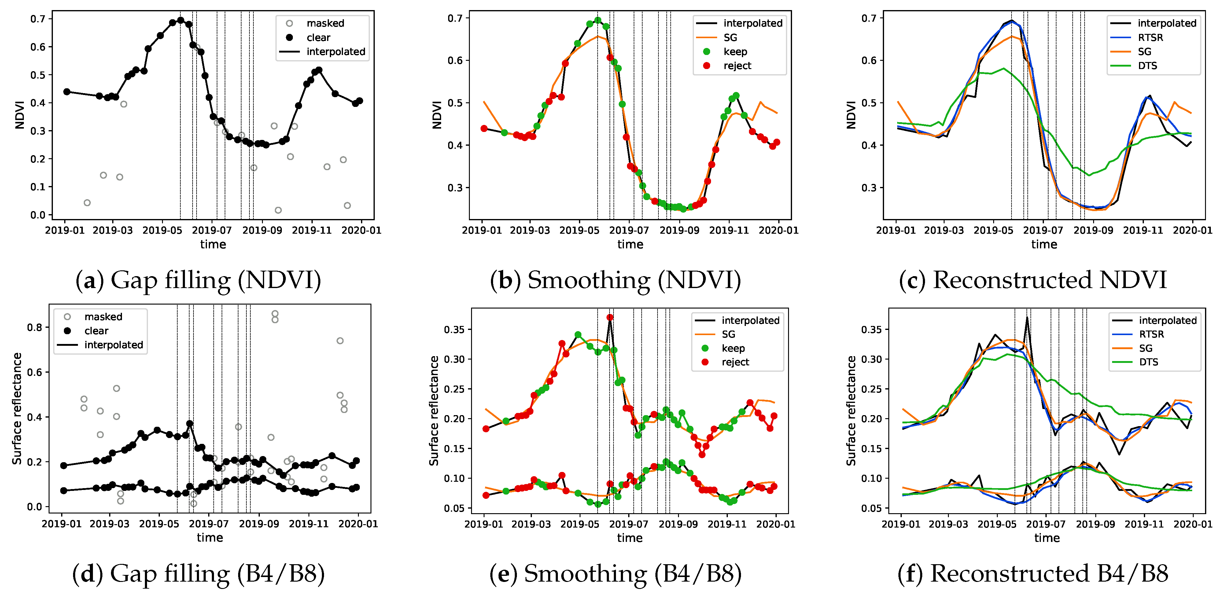
3.2. Adaptive Smoothing

The proposed reconstruction algorithm requires complete time series with contiguous observations in the temporal domain for each spectral band. Gaps due to missing or masked observations are filled with linearly interpolated values of clear observations. In case values are masked near the beginning and end of the time series, the nearest clear observation is extrapolated.

Even after interpolating the masked values, the reflectance values ${\mathrm{R}}_{\lambda ,i}$ (with $\lambda$ representing the wavelength and i the acquisition time) can still be noisy. For instance, the acquisition of 7 June 2019 corresponds to a “clear” observation (vertical line 2 in Figure 3). However, the reflectance in bands B4 and B8 is higher than expected, based on the previous and next clear observations (see Figure 3d). The isolated high reflectance can be interpreted as an outlier. This is also confirmed by the corresponding NDVI value, ${\mathrm{N}}_i$ (see Figure 3a). Similar to the time series of the interpolated spectral reflectance, ${\mathrm{R}}_{\lambda ,i}$, the time series for the interpolated NDVI value, ${\mathrm{N}}_i$, also shows an outlier for the acquisition from 7 June 2019. The isolated drop in NDVI is not compatible with a gradual change of vegetation and can be regarded as noisy. By inspecting Figure 3a, it is shown that the image scene indeed contains some cloud cover that could explain the noise.

Several algorithms for smoothing time series have been proposed in the literature, including the Whittaker smoother  [40], the Savitzky–Golay filter  [41], and its modifications  [20,42]. Because the proposed RTSR algorithm was inspired by the work in  [20], the same smoothing filter (Savitzky–Golay) was chosen here. It is important to note that other smoothing algorithms can easily be adopted in the proposed reconstruction method. Similar to the approach in  [20] to reconstruct the NDVI time series, a first Savitzky–Golay filter, referred to as ${\mathrm{SG}}^1$, creates the long-term change trend (represented by the orange lines in Figure 3). It has a relatively wide half-width of the smoothing window (7). This value is based on our own experiments and on values found in the literature  [20]. Likewise, the parameter for the polynomial degree was set to 2 for ${\mathrm{SG}}^1$ (suggested between 2 and 4 in  [20]). Larger values are supposed to better follow higher frequencies in the time series.

As illustrated in Figure 3b, the long-term change trend of the NDVI, ${\mathrm{SG}}^1\left({\mathrm{N}}_i\right)$, underestimates the NDVI values for the clear observations in May. Based on the assumption that relatively high NDVI values correspond to trustworthy observations, the upper NDVI envelope is expected to better reflect the dynamic changes of interest in the NDVI temporal profile  [20,21,22]. The acquisitions with a calculated NDVI above the long-term change trend (green dots) are therefore assumed to be more reliable than those with a calculated NDVI value below the long-term change trend (orange dots). Following this reasoning, the original spectral reflectance values ${\mathrm{R}}_{\lambda ,i}$ observed in May can be considered as reliable. Unlike the NDVI, however, the reflectance values are lower than the long-term change trend ${\mathrm{SG}}^1\left({\mathrm{R}}_{\lambda ,i}\right)$ (indicated in orange in Figure 3e). The assumption that clouds or poor atmospheric conditions depress NDVI values does not hold for the individual spectral bands. For instance, reflectance values in red and near infrared typically increase in case of cloud cover, but decrease in case of cloud shadow. Neither the upper nor the lower envelope reflect the dynamic changes of interest in the spectral reflectance temporal profile that would be observed in clear conditions. A different algorithmic approach for spectral reflectance was therefore developed, which is listed in Algorithm 1.

The reconstructed reflectance time series ${\widehat{\mathrm{R}}}_{\lambda ,i}$ is initialized as the long-term change trend ${\mathrm{SG}}^1\left({\mathrm{R}}_{\lambda ,i}\right)$. If, for a given acquisition i, the interpolated NDVI value ${\mathrm{N}}_i$ (calculated from the interpolated reflectance ${\mathrm{R}}_{\lambda ,i}$) shows a higher value than the current NDVI estimate ${\widehat{\mathrm{N}}}_i$ (calculated from the estimated reflectance ${\widehat{\mathrm{R}}}_{\lambda ,i}$), then the corresponding interpolated reflectance value ${\mathrm{R}}_{\lambda ,i}$ is assumed to be reliable and replaces the current estimate ${\widehat{\mathrm{R}}}_{\lambda ,i}$ (green dots in Figure 3e). Else, the current estimate ${\widehat{\mathrm{R}}}_{\lambda ,i}$ is retained in favor of the interpolated reflectance value ${\mathrm{R}}_{\lambda ,i}$ that is assumed to be noisy for the given acquisition i (e.g., orange dot in Figure 3e). By comparing the green and orange dots in both Figure 3b,e, it is shown that the decision which value to select (smoothed or interpolated version) is driven by the NDVI time series.

The algorithm proceeds by smoothing the retained spectral values with a second version of the SG filter, referred to as ${\mathrm{SG}}^2$. The smoothed values are then used for the next iteration. The reconstructed spectral reflectance time series ${\widehat{\mathrm{R}}}_{\lambda ,i}$ after the final iteration is shown in Figure 3c,f in blue. Different stopping criteria for number of iterations can be implemented. In [20], a fitting-effect index was proposed. Here, the number of iterations was experimentally fixed to five. More iterations did not further improve results. As a comparison, the reconstructed time series based on the dynamic temporal smoothing (DTS  [33]) method is also shown (in green).

Algorithm 1 Reflectance reconstruction algorithm

${\widehat{\mathrm{R}}}_{\lambda ,i}\leftarrow {\mathrm{SG}}^1\left({\mathrm{R}}_{\lambda ,i}\right)$  ▹ initialize reconstructed reflectance with long-term change trend while Stopping criterion not met (e.g., 5 iterations) do     if ${\widehat{\mathrm{N}}}_i<{\mathrm{N}}_i$ then                      ▹ observation is clear         ${\widehat{\mathrm{R}}}_{\lambda ,i}\leftarrow {\mathrm{R}}_{\lambda ,i}$                 ▹ update reconstructed reflectance     end if     ${\widehat{\mathrm{R}}}_{\lambda ,i}\leftarrow {\mathrm{SG}}^2\left({\widehat{\mathrm{R}}}_{\lambda ,i}\right)$             ▹ smoothen reconstructed reflectance end while

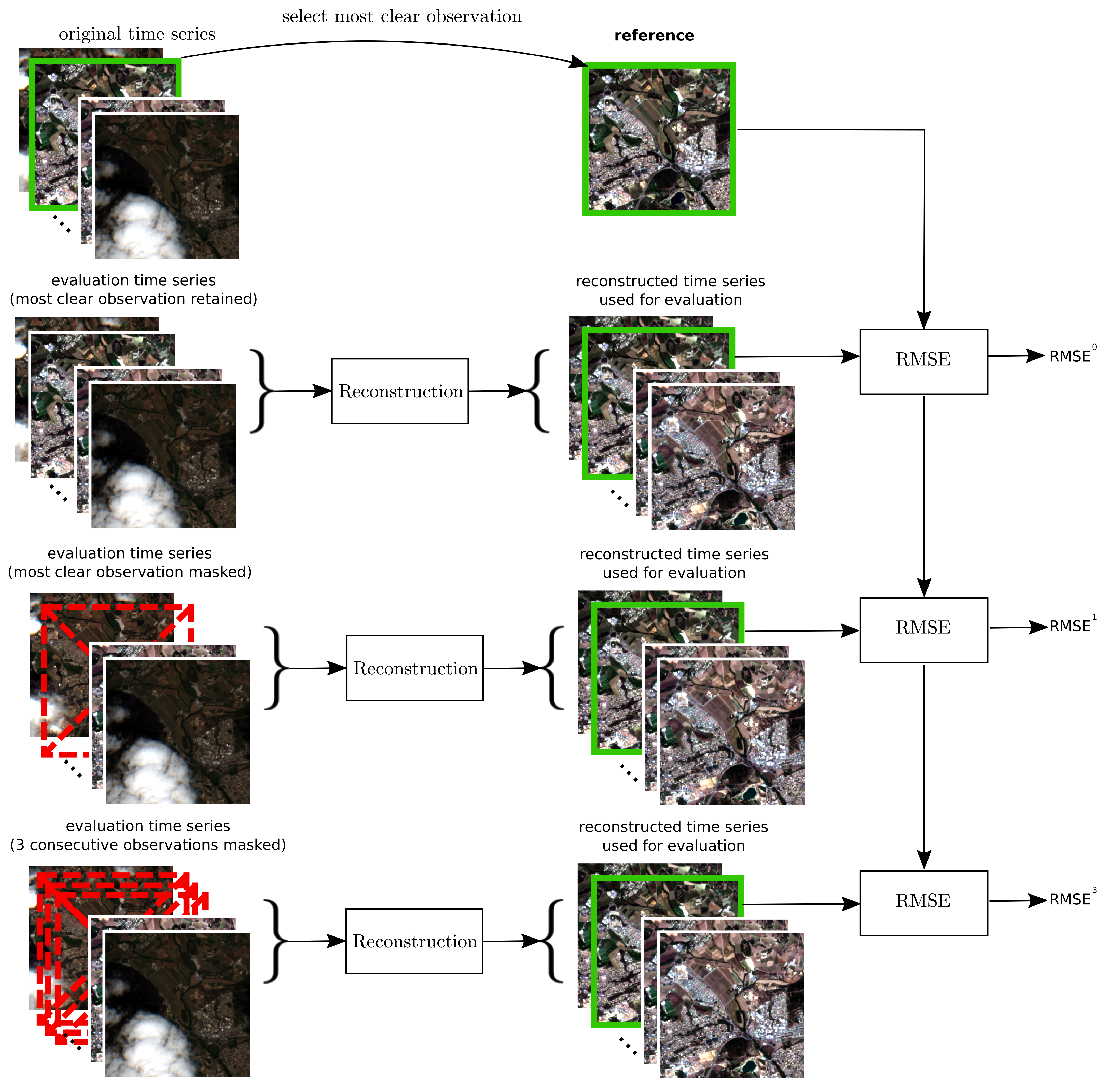
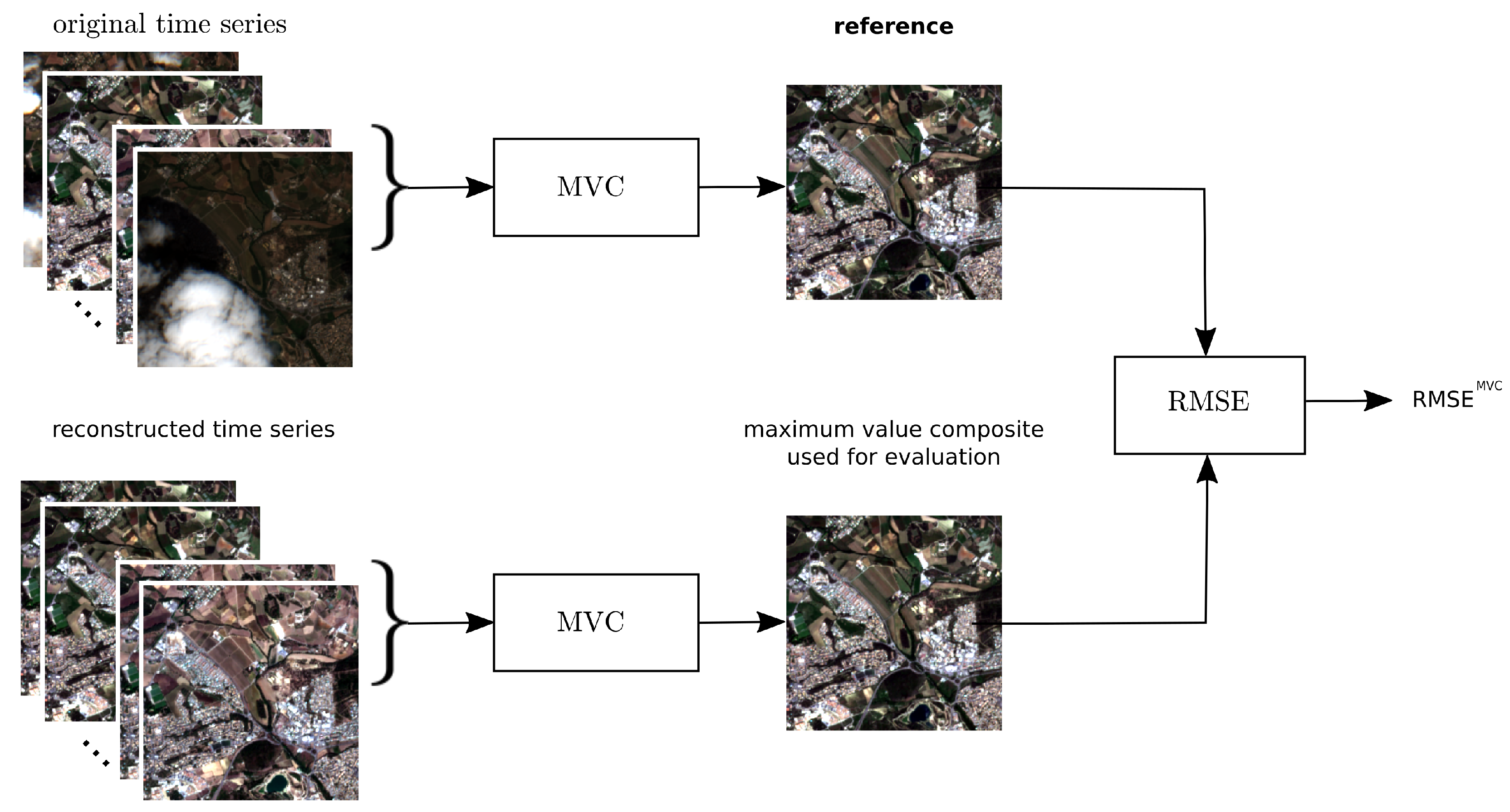
3.3. Evaluation Procedure

Different metrics were defined to evaluate the proposed reconstruction method, as requirements of a successful approach are also diverse. Noise should be reduced while changes related to vegetation dynamics of interest should be retained. A first metric was defined to quantify the smoothness, the time-series smoothness index (TSI) as proposed in [43]. It is calculated as the average absolute difference between the reconstructed reflectance value ${\widehat{\mathrm{R}}}_{\lambda ,i}$ at acquisition time i and the mean of the corresponding values before and after that acquisition. The difference is then averaged over all T acquisitions in the time series for each pixel (p):

$${\mathrm{TSI}}_{\lambda }\left(p\right)=\frac{1}{T}\sum _{i=1}^T|{\widehat{\mathrm{R}}}_{\lambda ,i}\left(p\right)-\frac{{\widehat{\mathrm{R}}}_{\lambda ,i-1}\left(p\right)+{\widehat{\mathrm{R}}}_{\lambda ,i-1}\left(p\right)}{2}|$$

(2)

Low TSI values indicate smooth time series and high TSI values indicate noisy time series for a specific spectral band $\lambda$. A similar evaluation method was conducted in [42,44]. Reconstruction methods with a high level of smoothing are expected to perform well on the TSI metric. However, they risk concealing the temporal changes of interest. Clear observations with low noise content should be represented in the reconstructed time series. A second evaluation metric was therefore based on the error between the reconstructed time series ${\widehat{\mathrm{R}}}_{\lambda ,i}$ and the original observation ${\mathrm{R}}_{\lambda ,i}$ in clear conditions ($i=i_{\mathrm{clear}}$). For each test site, $i_{\mathrm{clear}}$ was selected as the acquisition with the maximum number of clear pixels. The reconstructed time series ${\widehat{\mathrm{R}}}_{\lambda ,i}$ was then compared to the observed time series ${\mathrm{R}}_{\lambda ,i}$ at acquisition time $i_{\mathrm{clear}}$ (see top of Figure 4). Scatterplots were created per spectral band based on all clear pixels p in a test site (N in total). Pixels masked as not clear were not taken into account. In addition, the root mean squared error (${\mathrm{RMSE}}^0$) was calculated as:

$${\mathrm{RMSE}}_{\lambda }^0=\sqrt{\frac{{\sum }_{p=1}^N{({\widehat{\mathrm{R}}}_{\lambda ,i_{\mathrm{clear}}}\left(p\right)-{\mathrm{R}}_{\lambda ,i_{\mathrm{clear}}}\left(p\right))}^2}{N}}$$

(3)

Next, the most clear observation at acquisition time $i_{\mathrm{clear}}$ was masked, resulting in the metric ${\mathrm{RMSE}}^1$ (see center of Figure 4). This prevented the reconstruction algorithm using it as a trustworthy observation. Notice the extra gap that was introduced at acquisition time $i_{\mathrm{clear}}$ in addition to the existing gaps due to the already masked pixels. Similarly, ${\mathrm{RMSE}}^3$ was calculated by introducing three consecutive gaps in the time series, i.e., masking the most clear and its two surrounding observations (see bottom Figure 4).

A final evaluation metric, ${\mathrm{RMSE}}^{\mathrm{MVC}}$, was defined based on the maximum NDVI composite over the four-month period 1 May 2019–31 August 2019. This is illustrated in Figure 5. With an average of 41 available observations, the maximum NDVI value composite of the original time series is expected to minimize problems common to single-date remote sensing studies, such as cloud contamination, atmospheric attenuation, surface directional reflectance, and view and illumination geometry [19]. Reconstructed time series that retain high-quality pixel observations should have a similar maximum NDVI composite and result in low values of ${\mathrm{RMSE}}^{\mathrm{MVC}}$. On the other hand, higher values of ${\mathrm{RMSE}}^{\mathrm{MVC}}$ are expected for reconstruction methods that alter high-quality observations.

4. Results

The RTSR reconstruction algorithm was implemented in Python using the open source pyjeo [45] library. Processing was performed on the Big Data Analytics Platform (BDAP [46], the in-house storage and computing platform of the Joint Research Centre (JRC) of the European Commission (formerly known as the JEODPP). The results confirmed the potential of the adaptive smoothing using a vegetation index as a proxy for reliability of the reflectance values. A more detailed analysis of the test site near Montpellier is presented first, followed by an analysis of the metrics based on all test sites.

4.1. Evaluation of Test Site near Montpellier

In Figure 6, a subset of true color images for the reconstructed time series is shown. The subset corresponds to the eight acquisitions that are also shown in Figure 2 and illustrates qualitatively that cloudy and shadow pixels were reconstructed successfully.

Scatterplots for the spectral bands under study were then created for the same test site (Figure 7). The pixel values of the observed and the reconstructed time series are compared at acquisition time $i_{\mathrm{clear}}$ and visualized based on the kernel density estimate. It is shown that the proposed RTSR method outperforms SG and DTS. The linear regression model indicates a better fit for RTSR, with a strong correlation ($R^2$). In general, the SG- and DTS-reconstructed surface reflectance values over-estimated the observed surface reflectance value. This is also illustrated for the example pixel indicated by the red square in Figure 7 (except for DTS in B8). The time series in Figure 3f is based on the same pixel. Both SG- and DTS-reconstructed values for the clear observation on 23 May 2019 (first vertical line) indeed over-estimate the observation in B4 (lower graph). For this particular pixel and acquisition time, only SG over-estimated the observation in B8. The DTS-reconstructed surface reflectance in B8 was slightly lower than the clear observation, as can seen in the upper graph in Figure 3f. The RTSR reconstructed value shows little bias in any of the bands.

Furthermore, the $\mathrm{RMSE}$ based on the difference between the reconstructed and clear observations on 23 May 2019 was lower for RTSR than for the other two method, except for B8, where it was slightly larger the for this specific test site ($0.22$ with respect to $0.20$ for SG and DTS). However, it will be shown that for the majority of test sites, RTSR has a smaller RMSE for all tested bands.

4.2. Smoothness Index for Aggregated Test Sites

The smoothness for the three methods was evaluated by calculating TSI according to Equation (2). A cumulative frequency distribution representing all pixels aggregated for all test sites is shown in Figure 8. The results show little difference in the smoothness between the three reconstructed methods, with values for the 95 percentile that are almost identical. Most variation was found for spectral band B2, with smoothest results obtained for the non-adaptive Savitzky–Golay filter (SG) followed by the proposed RTSR and DTS. This is not surprising, as the SG-reconstructed time series represents the long-term change trend with a relatively wide half-width of the smoothing window. Both RTSR and DTS constrain the smoothing filter to capture dynamic changes of interest in vegetation.

4.3. Statistical Analysis of RMSE Metrics for Aggregated Test Sites

As shown by the box plot in Figure 9a, the RMSE for RTSR was found to be smaller than for SG and DTS for the majority of test sites. This was the case for all spectral bands. The difference was most distinct in the visual to near infrared part of the electomagnetic spectrum. Furthermore, in the short wave infrared (band B12), the minimum as well as the 25 percentile value (Q1) and the median value of the RMSE was minimum over all test sites for the proposed RTSR. However, for some test sites the RMSE was higher for the RTSR than for the SG without adjusting the smoothed value, as expressed by the slightly higher 75 percentile value (Q3) and upper whisker (${\mathrm{Q}}_3+1.5\times ({\mathrm{Q}}_3-{\mathrm{Q}}_1)$).

Following the addition of an extra gap in the time series, the three tested reconstruction methods performed more similarly (see Figure 9b). This can be expected given that the gap introduced exactly at acquisition time $i_{\mathrm{clear}}$ was also used as a reference. This trustworthy reflectance value in the time series was not available to adjust the smoothed value in the RTSR-reconstructed time series. Only clear observations from nearby acquisition times were able to contribute to the reconstructed time series. When introducing three consecutive gaps ($i_{\mathrm{clear}}-1,i_{\mathrm{clear}},i_{\mathrm{clear}}+1$), the difference between the compared methods was even more reduced, resulting in a comparable ${\mathrm{RMSE}}^3$ (see Figure 9c).

The results for the maximum-value composite over the four-month period 1 May 2019–31 August 2019 are shown in Figure 9d. The advantage of the proposed RTSR reconstruction method with respect to the other two reference methods is more expressed than in the previous metrics. A potential explanation is that only a single observation was used for the previous metrics. Although the most clear observation was selected, varying atmospheric conditions over the test site result in reflectance values that are not homogeneous. The pixels in this reference image contain some noise, which blurs differences in the evaluation metrics. As motivated in other evaluation studies that obtained reference data from the 10-year average (2011–2020) of NDVI data [25], aggregating data over time reduces noise in the reference data.

5. Discussion

5.1. Reference Data and Model Parameters

A major difficulty with the quantitative evaluation of reconstructed time series is the lack of reference data, which must match the test data in temporal, spatial, and spectral dimensions. Several studies have used modeled time series based on the average of multi-year data as a reference [13,25,47,48]. Noise is often added to the modeled reference time series to evaluate the performance of the reconstruction method. This assumes that the modeled data and added noise realistically represent the actual data that will be used for the model that is evaluated. In [25], reference data were obtained from the 10-year average (2011–2020) of NDVI data. The advantage of this is a relatively noise-free reference time series. Taking the average produces a smooth signal as frequent changes related to, e.g., bidirectional effects, crop-harvesting practice, and sudden changes in land cover, are smoothed out. Using averaged data as a reference risks favoring reconstruction algorithms that include a higher level of smoothing. There is a trade-off between reconstructing a smooth noise-free signal on one hand and retaining the original values of high-quality pixels that have been observed in clear conditions on the other. The optimal approach depends on the application. This is also reflected by the tuning parameters that often accompany reconstruction algorithms [20,33]. The idea is that users can then optimize these parameters for their application at hand. However, optimizing these parameters adds to the complexity of a fair comparison of different techniques. The DTS algorithm proposed in [33] contains 13 parameters, wherein the authors optimized these parameters using a reference dataset that captured a range of ecosystems and land use/cover types. They claim the parameters should therefore be fairly robust for applications using vegetation indices such as the EVI2 or NDVI. However, as reflectance values can have a different variance structure or dynamic ranges, different optimal parameters might apply.

In a production environment where products are created at regional and continental scales, the fine-tuning of parameters for individual areas can become tedious and potentially result in unwanted border effects between areas where parameters differ. Therefore, the parameters for the three methods under comparison were fixed. A first parameter of the proposed RTSR is related to the cloud buffer. Due to omission errors of the Sen2Cor cloud detection algorithm, not all cloudy pixels have been identified as such. The observation corresponding to the acquisition on 7 June 2019 (second vertical line in Figure 3) can also be considered as an outlier, but was identified by the SCL band as clear and thus not masked. Cloudy or shadow pixels that are not masked will not be interpolated during the gap-filling step of the method. The corresponding surface-reflectance values will be taken into account and add to the noise in the time series. Because omission errors are more frequent on cloud edges [49], an extra buffer around clouds masks is commonly used [38]. Here, a relatively small buffer of five pixels ($50\mathrm{m}$) was added. It was able to mask the observation corresponding to the acquisition on 12 June 2019 that was considered by the SCL band as clear (third vertical line in Figure 3). Using a larger buffer provides the potential to mask more pixels. For instance, buffer sizes of 100–300$\mathrm{m}$ were proposed in [38]. However, as suggested in [39], this also removes a large amount of usable imagery. The impact on the reconstructed time series will be reduced, because the observed surface-reflectance value near the cloud edge will most likely have a relatively low calculated NDVI value. The iterative RTSR algorithm will then reject this value and keep the smoothed value.

The parameters of the smoothing filters ${\mathrm{SG}}^1$ and ${\mathrm{SG}}^2$, were fixed based on the values found in the literature and experimental results. For the half-width of the smoothing window, values between 4 and 7 were suggested in [20]. Small values result in less smoothing with the risk of over-fitting the data points, whereas larger values risk not picking up important variations in the time series. For the first version of the SG filter, ${\mathrm{SG}}^1$, a value of 7 was selected with a polynomial degree of 2 (suggested between 2 and 4 in [20]). This creates a relatively smooth signal that is able to represent the slowly varying long-term change trend. A lower filter width and a higher polynomial degree was set for ${\mathrm{SG}}^2$ (3 and 3 instead of 4 and 2) so that important variations potentially smoothed out with ${\mathrm{SG}}^1$, can still be picked up by the iterative algorithm. This is illustrated in Figure 3c,f. In contrast to the long-term change trend (in orange), the reconstructed time series (in blue) represents well the original values near the green peak (23 May 2019). The reconstruction based on DTS (in green) neither represents the original values near the maximum nor the minimum greenness. The relatively poor performance of DTS is potentially due its application to surface reflectance data. Although the code in [32] is claimed to be applicable to time series of satellite observations in general, the DTS presented in [33] was applied to EVI2 time series and involved an adjustment to the upper envelope. As for the NDVI, the assumption is that relatively high values correspond to a trustworthy observation. This assumption does not hold for surface reflectance. The DTS-reconstructed time series was obtained with the original code in [32] without this adjustment. Nevertheless, for most test sites the RMSE values of DTS are still in line with the RMSE values obtained in other studies. In [28], a reconstruction algorithm on Sentinel-2 surface reflectance data was evaluated using a metric similar to ${\mathrm{RMSE}}^0$ and obtained RMSE values of $0.0426$ (B2), $0.0407$ (B3), $0.0405$ (B4), and $0.0449$ (B8). In [30], reconstructed MODIS Terra MOD09A1 data were evaluated on cloud-free MODIS Aqua MYD09A1 data: $0.0366$ (red band), $0.0519$ (near infrared band), and $0.0499$ (short-wave infrared band).

5.2. Limitations

The relatively low number of test sites (100) and the restricted geographic location (Europe) limit the importance of the evaluation results. Rather than showing the superiority of the proposed RTSR method, the objective of the evaluation was to show the potential of dynamic smoothing where the time series approaches the trustworthy observations. The smoothing method can hereby be adopted from other methods, such as that proposed in DTS. A diverse set evaluation metric was hereby selected. Results of the TSI showed minor differences in smoothness for the three methods under comparison. All three methods were also able to fill gaps in the time series, which is driven by interpolating clear observations near the missing values. The strength of the proposed RTSR is that in addition to producing a smooth reconstructed time series, it is capable of retaining trustworthy observations in the original time series.

A number of limitations of the proposed RTSR method do apply. The time series to be reconstructed must include the spectral bands to calculate the index used as a proxy for the reliability of observations (e.g., the B4 and B8 bands of the Sentinel-2 sensor in the case of NDVI). Another limitation is the assumption that clouds or poor atmospheric conditions depress NDVI values [18]. This holds mostly for vegetated land but not for all land cover types. Clear observations of water bodies, for example, can result in lower NDVI values than cloudy observations. This is not a limitation of the method, but of the proxy used for trustworthy observations. The proxy can be adapted, for example, by distinguishing pixels using a water mask. Instead of NDVI, water surface-reflectance values in the near infrared band can be compared in the iterative algorithm. Clear water pixels usually have lower reflectance values in this part of the electromagnetic spectrum than clouds. When applying the RTSR reconstruction algorithm to create analysis-ready data for other applications beyond vegetation monitoring, the proxy could be adapted in this way. Further evaluation will be needed and is to be part of future research.

The Savitzky–Golay smoothing filter used in the reconstruction algorithm imposes another limitation. The RTSR reconstruction method requires a time series of at least 15 observations, i.e., the full width of the Savitzky–Golay filter, to obtain the long-term change trend curve. A longer time series is needed in practice to improve the results, typically 20 observations or more. In the case of Sentinel-2 acquisitions, this corresponds to a seasonal to annual coverage. The maximum length of the time series is only constrained by the memory resources available, as our implementation reads the entire time series in memory. Because the RTSR algorithm is a pixel-wise operation and requires no spatial contextual information, there is no upper limit in the spatial dimension. The image can be split into smaller tiles that can be run independently in parallel. Tiles can be made as small as needed to fit in the available memory. For instance, the test sites of 256 by 256 pixels and covering 62 acquisitions can be processed with less than $2\mathrm{GB}$ of memory.

Due to the extent of the smoothing window size, there is an edge effect inherent to the filtering process that impacts the first and last observations of the reconstructed time series. In this study, the acquisition period was extended by one month before and after the period of interest. The respective observations (December 2018 and January 2020) were afterwards removed from the reconstructed time series. This approach is not suited for near real-time applications. The Whittaker smoother has a number of advantages over the SG filter [21,40,50,51]. It employs only past observations and would be a good candidate for the smoothing filter, in particular for near real-time applications. This will be part of future research. Another interesting topic is the effect of the cloud mask on the reconstructed time series and to investigate whether more sophisticated cloud masks can improve results.

6. Conclusions

A spectral reflectance time-series reconstruction (RTSR) method has been proposed to reconstruct optical remote-sensing time-series data that are hampered by missing or noisy observations due to varying atmospheric conditions. This method differs from existing approaches in that it adjusts smoothed values of surface reflectance values to approach those of trustworthy observations, using a vegetation index as a proxy for reliability. The results show that the RTSR method is effective in retaining trustworthy observations in the original time series, with RMSE values in the order of $0.01$ to $0.03$ in terms of surface reflectance. The method was evaluated on 100 sites in Europe, with a focus on vegetation. The Savitzky–Golay filter was employed herein as the smoothing algorithm, but other filters can also be used. The potential of this method is substantial now that optical remote-sensing data have become publicly available at a finer spatial and temporal resolution. We hope that this study will encourage further research in this area, and that the RTSR method will be applied to create analysis-ready data for other applications beyond vegetation monitoring.

References

1. Drusch, M.; Del Bello, U.; Carlier, S.; Colin, O.; Fernandez, V.; Gascon, F.; Hoersch, B.; Isola, C.; Laberinti, P.; Martimort, P.; et al. Sentinel-2: ESA’s Optical High-Resolution Mission for GMES Operational Services. Remote Sens. Environ. 2012, 120, 25–36. [Google Scholar] [CrossRef]
2. Ma, C.; Liu, M.; Ding, F.; Li, C.; Cui, Y.; Chen, W.; Wang, Y. Wheat growth monitoring and yield estimation based on remote sensing data assimilation into the SAFY crop growth model. Sci. Rep. 2022, 12, 5473. [Google Scholar] [CrossRef]
3. Lambert, J.; Drenou, C.; Denux, J.P.; Balent, G.; Cheret, V. Monitoring forest decline through remote sensing time series analysis. Gisci. Remote Sens. 2013, 50, 437–457. [Google Scholar] [CrossRef]
4. Griffiths, P.; Nendel, C.; Pickert, J.; Hostert, P. Towards national-scale characterization of grassland use intensity from integrated Sentinel-2 and Landsat time series. Remote Sens. Environ. 2020, 238, 111124. [Google Scholar] [CrossRef]
5. Moreno-Martínez, Á.; Izquierdo-Verdiguier, E.; Maneta, M.P.; Camps-Valls, G.; Robinson, N.; Muñoz-Marí, J.; Sedano, F.; Clinton, N.; Running, S.W. Multispectral high resolution sensor fusion for smoothing and gap-filling in the cloud. Remote Sens. Environ. 2020, 247, 111901. [Google Scholar] [CrossRef] [PubMed]
6. Kempeneers, P.; Sedano, F.; Piccard, I.; Eerens, H. Data Assimilation of PROBA-V 100 and 300 m. IEEE J. Sel. Top. Appl. Earth Obs. Remote. Sens. 2016, 9, 3314–3325. [Google Scholar] [CrossRef]
7. Sedano, F.; Kempeneers, P.; Hurtt, G. A Kalman Filter-Based Method to Generate Continuous Time Series of Medium-Resolution NDVI Images. Remote Sens. 2014, 6, 12381–12408. [Google Scholar] [CrossRef]
8. Inglada, J.; Vincent, A.; Arias, M.; Marais-Sicre, C. Improved Early Crop Type Identification By Joint Use of High Temporal Resolution SAR Furthermore, Optical Image Time Series. Remote Sens. 2016, 8, 362. [Google Scholar] [CrossRef]
9. Lasko, K. Gap Filling Cloudy Sentinel-2 NDVI and NDWI Pixels with Multi-Frequency Denoised C-Band and L-Band Synthetic Aperture Radar (SAR), Texture, and Shallow Learning Techniques. Remote Sens. 2022, 14, 4224. [Google Scholar] [CrossRef]
10. Xiong, S.; Du, S.; Zhang, X.; Ouyang, S.; Cui, W. Fusing Landsat-7, Landsat-8 and Sentinel-2 surface reflectance to generate dense time series images with 10 m spatial resolution. Int. J. Remote Sens. 2022, 43, 1630–1654. [Google Scholar] [CrossRef]
11. Inglada, J.; Arias, M.; Tardy, B.; Morin, D.; Valero, S.; Hagolle, O.; Dedieu, G.; Sepulcre, G.; Bontemps, S.; Defourny, P. Benchmarking of algorithms for crop type land-cover maps using Sentinel-2 image time series. In Proceedings of the 2015 IEEE International Geoscience and Remote Sensing Symposium (IGARSS), Milan, Italy, 26–31 July 2015; pp. 3993–3996. [Google Scholar] [CrossRef]
12. Saunier, S.; Pflug, B.; Lobos, I.M.; Franch, B.; Louis, J.; De Los Reyes, R.; Debaecker, V.; Cadau, E.G.; Boccia, V.; Gascon, F.; et al. Sen2Like: Paving the Way towards Harmonization and Fusion of Optical Data. Remote Sens. 2022, 14, 3855. [Google Scholar] [CrossRef]
13. Hird, J.N.; McDermid, G.J. Noise reduction of NDVI time series: An empirical comparison of selected techniques. Remote Sens. Environ. 2009, 113, 248–258. [Google Scholar] [CrossRef]
14. Moreno-Martínez, Á.; García-Haro, F.J.; Martínez, B.; Gilabert, M.A. Noise Reduction and Gap Filling of fAPAR Time Series Using an Adapted Local Regression Filter. Remote Sens. 2014, 6, 8238–8260. [Google Scholar] [CrossRef]
15. Meroni, M.; d’Andrimont, R.; Vrieling, A.; Fasbender, D.; Lemoine, G.; Rembold, F.; Seguini, L.; Verhegghen, A. Comparing land surface phenology of major European crops as derived from SAR and multispectral data of Sentinel-1 and -2. Remote Sens. Environ. 2021, 253, 112232. [Google Scholar] [CrossRef] [PubMed]
16. Karkauskaite, P.; Tagesson, T.; Fensholt, R. Evaluation of the Plant Phenology Index (PPI), NDVI and EVI for Start-of-Season Trend Analysis of the Northern Hemisphere Boreal Zone. Remote Sens. 2017, 9, 485. [Google Scholar] [CrossRef]
17. Tucker, C.J. Red and photographic infrared linear combinations for monitoring vegetation. Remote Sens. Environ. 1979, 8, 127–150. [Google Scholar] [CrossRef]
18. Goward, S.N.; Markham, B.; Dye, D.G.; Dulaney, W.; Yang, J. Normalized difference vegetation index measurements from the Advanced Very High Resolution Radiometer. Remote Sens. Environ. 1991, 35, 257–277. [Google Scholar] [CrossRef]
19. Holben, B.N. Characteristics of maximum-value composite images from temporal AVHRR data. Int. J. Remote Sens. 1986, 7, 1417–1434. [Google Scholar] [CrossRef]
20. Chen, J.; Jönsson, P.; Tamura, M.; Gu, Z.; Matsushita, B.; Eklundh, L. A simple method for reconstructing a high-quality NDVI time-series data set based on the Savitzky–Golay filter. Remote Sens. Environ. 2004, 91, 332–344. [Google Scholar] [CrossRef]
21. Atzberger, C.; Eilers, P.H. A time series for monitoring vegetation activity and phenology at 10-daily time steps covering large parts of South America. Int. J. Digit. Earth 2011, 4, 365–386. [Google Scholar] [CrossRef]
22. Liu, R.; Shang, R.; Liu, Y.; Lu, X. Global evaluation of gap-filling approaches for seasonal NDVI with considering vegetation growth trajectory, protection of key point, noise resistance and curve stability. Remote Sens. Environ. 2017, 189, 164–179. [Google Scholar] [CrossRef]
23. Huete, A.; Justice, C.; Van Leeuwen, W. MODIS vegetation index (MOD13). Algorithm Theor. Basis Doc. 1999, 3, 295–309. [Google Scholar]
24. Maisongrande, P.; Duchemin, B.; Dedieu, G. VEGETATION/SPOT: An operational mission for the Earth monitoring; presentation of new standard products. Int. J. Remote Sens. 2004, 25, 9–14. [Google Scholar] [CrossRef]
25. Li, S.; Xu, L.; Jing, Y.; Yin, H.; Li, X.; Guan, X. High-quality vegetation index product generation: A review of NDVI time series reconstruction techniques. Int. J. Appl. Earth Obs. Geoinf. 2021, 105, 102640. [Google Scholar] [CrossRef]
26. Zhu, Z.; Zhang, J.; Yang, Z.; Aljaddani, A.H.; Cohen, W.B.; Qiu, S.; Zhou, C. Continuous monitoring of land disturbance based on Landsat time series. Remote Sens. Environ. 2020, 238, 111116. [Google Scholar] [CrossRef]
27. Dwyer, J.L.; Roy, D.P.; Sauer, B.; Jenkerson, C.B.; Zhang, H.K.; Lymburner, L. Analysis Ready Data: Enabling Analysis of the Landsat Archive. Remote Sens. 2018, 10, 1363. [Google Scholar] [CrossRef]
28. Yan, L.; Roy, D.P. Spatially and temporally complete Landsat reflectance time series modelling: The fill-and-fit approach. Remote Sens. Environ. 2020, 241, 111718. [Google Scholar] [CrossRef]
29. Yang, K.; Luo, Y.; Li, M.; Zhong, S.; Liu, Q.; Li, X. Reconstruction of Sentinel-2 Image Time Series Using Google Earth Engine. Remote Sens. 2022, 14, 4395. [Google Scholar] [CrossRef]
30. Xiao, Z.; Liang, S.; Wang, T.; Liu, Q. Reconstruction of Satellite-Retrieved Land-Surface Reflectance Based on Temporally-Continuous Vegetation Indices. Remote Sens. 2015, 7, 9844–9864. [Google Scholar] [CrossRef]
31. Xiao, Z.; Liang, S.; Tian, X.; Jia, K.; Yao, Y.; Jiang, B. Reconstruction of Long-Term Temporally Continuous NDVI and Surface Reflectance From AVHRR Data. IEEE J. Sel. Top. Appl. Earth Obs. Remote Sens. 2017, 10, 5551–5568. [Google Scholar] [CrossRef]
32. Dynamic Temporal Smoothing (DTS). Available online: https://github.com/jgrss/satsmooth (accessed on 28 October 2022).
33. Graesser, J.; Stanimirova, R.; Friedl, M.A. Reconstruction of satellite time series with a dynamic smoother. IEEE J. Sel. Top. Appl. Earth Obs. Remote Sens. 2022, 15, 1803–1813. [Google Scholar] [CrossRef]
34. d’Andrimont, R.; Claverie, M.; Kempeneers, P.; Muraro, D.; Yordanov, M.; Peressutti, D.; Batič, M.; Waldner, F. AI4Boundaries: An open AI-ready dataset to map field boundaries with Sentinel-2 and aerial photography. Earth Syst. Sci. Data 2023, 15, 317–329. [Google Scholar] [CrossRef]
35. Buttner, G.; Feranec, J.; Jaffrain, G.; Mari, L.; Maucha, G.; Soukup, T. The CORINE land cover 2000 project. EARSeL eProceedings 2004, 3, 331–346. [Google Scholar]
36. Copernicus Open Access Hub. Available online: https://scihub.copernicus.eu/dhus (accessed on 16 December 2021).
37. Sentinel-2 Level-2A Algorithm Theoretical Basis Document. Available online: https://sentinels.copernicus.eu/documents/247904/446933/Sentinel-2-Level-2A-Algorithm-Theoretical-Basis-Document-ATBD.pdf (accessed on 12 September 2022).
38. Zekoll, V.; Main-Knorn, M.; Alonso, K.; Louis, J.; Frantz, D.; Richter, R.; Pflug, B. Comparison of Masking Algorithms for Sentinel-2 Imagery. Remote Sens. 2021, 13, 137. [Google Scholar] [CrossRef]
39. Hughes, M.J.; Kennedy, R. High-Quality Cloud Masking of Landsat 8 Imagery Using Convolutional Neural Networks. Remote Sens. 2019, 11, 2591. [Google Scholar] [CrossRef]
40. Whittaker, E.T. On a new method of graduation. Proc. Edinb. Math. Soc. 1922, 41, 63–75. [Google Scholar] [CrossRef]
41. Savitzky, A.; Golay, M.J. Smoothing and differentiation of data by simplified least squares procedures. Anal. Chem. 1964, 36, 1627–1639. [Google Scholar] [CrossRef]
42. Verger, A.; Baret, F.; Weiss, M. A multisensor fusion approach to improve LAI time series. Remote Sens. Environ. 2011, 115, 2460–2470. [Google Scholar] [CrossRef]
43. Weiss, M.; Baret, F.; Garrigues, S.; Lacaze, R. LAI and fAPAR CYCLOPES global products derived from VEGETATION. Part 2: Validation and comparison with MODIS collection 4 products. Remote Sens. Environ. 2007, 110, 317–331. [Google Scholar] [CrossRef]
44. Claverie, M.; Ju, J.; Masek, J.G.; Dungan, J.L.; Vermote, E.F.; Roger, J.C.; Skakun, S.V.; Justice, C. The Harmonized Landsat and Sentinel-2 surface reflectance data set. Remote Sens. Environ. 2018, 219, 145–161. [Google Scholar] [CrossRef]
45. Kempeneers, P.; Pesek, O.; De Marchi, D.; Soille, P. pyjeo: A Python Package for the Analysis of Geospatial Data. ISPRS Int. J. Geo-Inf. 2019, 8, 461. [Google Scholar] [CrossRef]
46. Soille, P.; Burger, A.; De Marchi, D.; Kempeneers, P.; Rodriguez, D.; Syrris, V.; Vasilev, V. A versatile data-intensive computing platform for information retrieval from big geospatial data. Future Gener. Comput. Syst. 2018, 81, 30–40. [Google Scholar] [CrossRef]
47. Xu, L.; Li, B.; Yuan, Y.; Gao, X.; Zhang, T. A Temporal-Spatial Iteration Method to Reconstruct NDVI Time Series Datasets. Remote Sens. 2015, 7, 8906–8924. [Google Scholar] [CrossRef]
48. Zhou, J.; Jia, L.; Menenti, M.; Gorte, B. On the performance of remote sensing time series reconstruction methods–A spatial comparison. Remote Sens. Environ. 2016, 187, 367–384. [Google Scholar] [CrossRef]
49. Skakun, S.; Wevers, J.; Brockmann, C.; Doxani, G.; Aleksandrov, M.; Batič, M.; Frantz, D.; Gascon, F.; Gómez-Chova, L.; Hagolle, O.; et al. Cloud Mask Intercomparison eXercise (CMIX): An evaluation of cloud masking algorithms for Landsat 8 and Sentinel-2. Remote Sens. Environ. 2022, 274, 112990. [Google Scholar] [CrossRef]
50. Shao, Y.; Lunetta, R.S.; Wheeler, B.; Iiames, J.S.; Campbell, J.B. An evaluation of time-series smoothing algorithms for land-cover classifications using MODIS-NDVI multi-temporal data. Remote Sens. Environ. 2016, 174, 258–265. [Google Scholar] [CrossRef]
51. Schmid, M.; Rath, D.; Diebold, U. Why and How Savitzky–Golay Filters Should Be Replaced. ACS Meas. Sci. Au 2022, 2, 185–196. [Google Scholar] [CrossRef]
Figure 1. Test sample: 100 sites of 2560 by 2560 m distributed over six European countries (Austria, Spain, France, Netherlands, Slovenia, and Sweden).
Remotesensing 15 02303 g001
Figure 2. True color images (bands B4, B3, B2) for a subset of the time series acquired with Sentinel-2 under various atmospheric conditions (selected acquisition dates: 23 May 2019, 7 June 2019, 12 June 2019, 7 July 2019, 17 July 2019, 6 August 2019, 16 August 2019, 21 August 2019). The red square area corresponds to an agriculture field near Montpellier, France (43°39′53.64′′N, 3°54′47.88′′E).
Remotesensing 15 02303 g002
Figure 3. Reconstruction of NDVI (top) and spectral bands B4 and B8 (bottom). Vertical lines correspond to selected acquisition dates in Figure 2. Masked pixels are interpolated to fill gaps in the time series (left column). The iterative reconstruction process (middle column) checks whether observations are trustworty (green) or not (orange) based on the NDVI value. The NDVI values in green that are above the orange long-term change trend curve (SG) are retained for the next iteration. Those in red that are below will be replaced by the corresponding values on SG curve. Reconstructed time series (right column) for the proposed RTSR method (in blue) compared to SG (orange) and the dynamic temporal smoothing (DTS, in green).
Remotesensing 15 02303 g003
Figure 4. Metrics RMSE 0 , RMSE 1 , and RMSE 3 to evaluate the reconstruction method on the ability to retain high-quality pixels using the most clear observation as a reference.
Remotesensing 15 02303 g004
Figure 5. Evaluation metric based on the maximum NDVI value composite over the four-month period 1 May 2019–31 August 2019.
Remotesensing 15 02303 g005
Figure 6. Reconstructed true color images corresponding to the acquisitions in Figure 2.
Remotesensing 15 02303 g006
Figure 7. Scatterplot comparing the pixel values of the observed and the reconstructed time series for each spectral bands at acquisition time i clear . The red square corresponds to the pixel that is also indicated in Figure 2 and Figure 6. The RMSE value, slope, intercept, and coefficient of determination ( R 2 ) of the linear regression are also shown.
Remotesensing 15 02303 g007
Figure 8. Cumulative frequency distribution for the time-series smoothness index in the visible (B2, B3, B4), near infrared (B8) and short-wave infrared (B12) calculated for three reconstruction methods (SG, DTS, and the proposed RTSR). Small values indicate smoother time series. The 95 percentile is indicated in brackets.
Remotesensing 15 02303 g008
Figure 9. RMSE based on the difference between the reconstructed image and the original observation for the most clear observation ( RMSE 0 , RMSE 1 , and RMSE 3 ) and for the maximum NDVI value composite over a four-month period (1 May 2019–31 August 2019).
Remotesensing 15 02303 g009
Disclaimer/Publisher’s Note: The statements, opinions and data contained in all publications are solely those of the individual author(s) and contributor(s) and not of MDPI and/or the editor(s). MDPI and/or the editor(s) disclaim responsibility for any injury to people or property resulting from any ideas, methods, instructions or products referred to in the content.