1. Introduction
By extracting the characteristic parameters implied by the reflection waveform of Light Detection and Ranging (LiDAR) point cloud data as the basis for land cover classification, the distribution and type of buildings and vegetation on the ground surface can be understood. It can be used for disaster prevention during normal times and can effectively and quickly detect changes in surface objects and assist in disaster rescue when disasters occur. With the continuous improvement of LiDAR technology, its point cloud data can be used to interpret and classify the results, which can be combined with engineering and production management. Engineering inspection and land dispute handling can improve the efficiency of personnel work and also reduce the occurrence of hazardous factors.
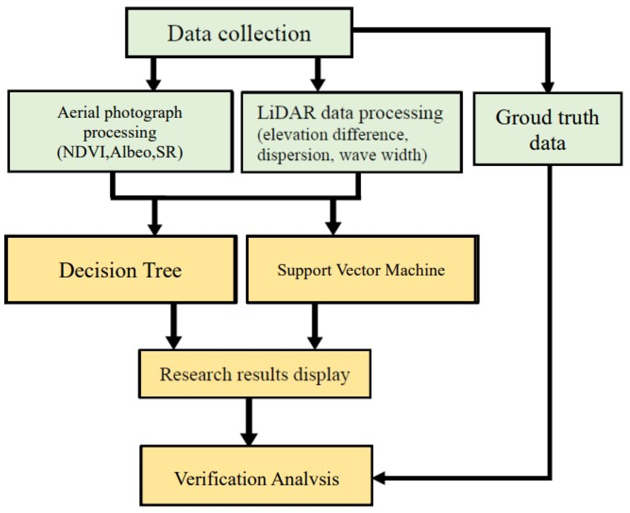
This study is mainly based on the analysis of LiDAR data and aerial photographs by extracting their spectral and geometric features as object-oriented classification parameters and classifying parameters based on feature combinations and self-defined elevations. The classification of land cover objects is completed with decision tree classification methods (DT) and support vector machine classification methods (SVM). The classification results of each feature combination are compared and validated. The research workflow is shown in
Figure 1.
The purpose of this study is to perform land cover classification using airborne LiDAR data and aerial photographs. By extracting the geometric characteristic parameters of the airborne LiDAR data and the spectral characteristic parameters of the aerial photographs, object-oriented classification software is used to analyze and classify the land cover characteristics. The land cover in the study area is divided into six categories: artificial ground, buildings, bare ground, grassland, trees, and planted shrubs. The research is divided into three stages. The first stage is to use the height difference, dispersion, and wavelength extracted from the LiDAR data to classify land features and then to distinguish the parameters from the height difference to perform the DT classification and accuracy evaluation. In the second stage, in addition to using LiDAR data, aerial photographs are added to the DT classification and accuracy evaluation to improve the classification accuracy. In the third stage, the SVM classification method is used for classification to compare the classification results of different classification methods.
The related work is discussed below. The data collection and methods are explained in
Section 2. Then,
Section 3 demonstrates the experimental results and discussion. Finally,
Section 4 presents the conclusions and suggestions of this paper.
The airborne LiDAR system has the advantages of high precision, high resolution, high automation, and high efficiency. It has become the mainstream trend of large-scale three-dimensional surface data surveying and mapping. Its multiple reflection echo characteristics can simultaneously obtain accurate three-dimensional coordinates of the ground and its covering (vegetation and buildings) [
1,
2]. The airborne LiDAR system mainly includes a Position and Orientation System (POS), laser scanner, and system controller. It can be applied to high-precision Digital Terrain Model (DTM) [
3], Digital Surface Model (DSM) measurement [
4], forest resource survey [
5], power line detection [
6], 3D city modeling [
7], and other purposes.
Aerial photogrammetry technology has a fairly developed ability to detect land cover, and it is a remote sensing measurement method. The measurer does not need to touch the object to be measured in person and can measure or sense the object to be measured from the air only by using the detection tool (such as cameras and laser scanners), which breaks through the limitation of ground investigation and measurement by human power in the past. It can also obtain the shape, position, and characteristics of various objects in the three-dimensional space, which meets visual needs. The scope of application includes land cover classification [
8], forest monitoring [
9,
10], plant growth analysis [
11], and land disaster assessment [
12].
Remote sensing is a technique for measuring and analyzing target acquisition data through indirect contact. It mainly detects and measures the properties of objects (such as state, area, and characteristics) through the conduction of electromagnetic waves. Through electromagnetic wave observation, different reflection characteristics of objects are used to identify and analyze the targets and phenomena on the surface. For the detection results of different wavelengths, soil, plants, and water have different reflection values. These characteristics can be used to carry out various scientific and land cover classification research [
13].
Remote sensing images are mainly divided into panchromatic images, multispectral images, and hyperspectral images. In the remote sensing analysis process, spectral sensors play a key role in image understanding and feature visualization. The image obtained by the sensor can be used for artificial photointerpretation and computer quantitative analysis. The reason why human eyes can perceive the color changes around them is that after the sunlight irradiates objects, the light is reflected to the human eyes through the surface of the objects, so the eyes can perceive different colors. Sunlight is composed of different electromagnetic waves, and the wavelength of visible light that can be seen by the human eye is about 0.4–0.7 µm. In addition to visible light, there are still many electromagnetic waves of different wavelengths in sunlight, such as γ-rays, χ-rays, and ultraviolet rays with shorter wavelengths, infrared rays, thermal infrared rays, and radio waves with longer wavelengths. Therefore, various scientific research can be carried out by analyzing the electromagnetic spectrum reflected by surface objects.
The Normalized Difference Vegetation Index (NDVI) is the most commonly used index for green plant exploration [
14]. As green plants grow more vigorously, chlorophyll absorbs more red light and reflects near-infrared light more strongly. Using the principle that the difference between the two is greater, it is composed of the ratio of the subtraction and addition of the two bands. NDVI is a ratio without units, and its value ranges from −1.0 to 1.0. The larger the value, the more lush the green vegetation growth. The expression formula is as follows:
2. Data Collection and Methods
2.1. Research Area
The research area of this paper is located in some mountainous areas of Taiping District, Taichung City, Taiwan. The size of the area is 400 × 400 m, and the average altitude of the study area is about 600 m. The types of land cover within the scope include houses, dormitories, various types of trees, roads, rivers, grasslands, bare land, and concrete open spaces. Among them, the height of the buildings is mostly less than two floors, and the trees can be mainly divided into large trees (banyan, longan, and litchi) and small shrubs (carambola).
2.2. Data Collection and Processing
2.2.1. Airborne LiDAR
It is stated in [
15] that the traditional pulsed multiple-echo LiDAR and full-waveform LiDAR data are used to study the performance of classification results, and a considerable number of parameters extracted from waveforms are compared. Using full-waveform LiDAR data can help improve the accuracy of land cover classification compared to pulsed multiple-echo LiDAR.
In this study, the LiDAR data was scanned using the Riegl LMS-Q680i airborne LiDAR instrument to scan some mountainous areas in Taiping District, Taichung City, Taiwan, with an average flight altitude of 1200 m.
LMS-Q680i is a full-waveform airborne LiDAR system manufactured by Austrian manufacturer Riegl. It has the functions of Multiple-Time-Around (MTA) and digital full-waveform analysis. It has good linear scanning, scanning speed of 266,000 points/second in point arrangement mode, 10–200 scanning lines/second, full-waveform technology, and accuracy up to 20 mm. The system is mainly composed of three parts: positioning and orientation system, laser scanner, and controller. Among them, the orientation system obtains three-dimensional coordinates by direct geometric alignment technology and integrated satellite positioning system technology. Together with the three-axis deflection angle and acceleration information measured by the precision inertial attitude instrument, it directly provides the precise track positioning function during the flight.
Riegl uses the SDF format to store waveform information, which is not a public format. Riegl has also customized a binary file format for recording processed waveform information and parameters, and the file format records LiDAR information. These include time, range, angle, three-dimensional coordinates (X, Y, Z), amplitude, wave width, return number, total number of returns, and class. The three-dimensional coordinates, amplitude, and wave width values used in this study are LiDAR parameters converted by Riegl’s original program. The main converted formats are LAS1.2 format [
16] and ASCII files.
The LiDAR parameters mainly used in this study include parameter values such as the wave width value. Matlab, C#, and other programming languages were used to extract point cloud coordinates (X, Y, Z), elevation difference, dispersion, and wave width from ASCII files, and the parameters were loaded into the classification software for operation.
- 1.
Elevation Difference (dz)
Elevation difference is a parameter representing terrain roughness, and its difference is DSM minus DTM. If the topographic elevation fluctuation of the research area is not large, the influence of topography may not be considered. If the research area is located in a place with large terrain fluctuations, the vertical height difference to the terrain surface must be used.
- 2.
Dispersion (sigma)
Dispersion is a parameter that can represent the discreteness of the terrain. It is set by the program to search for pixels that can be found within a certain spherical radius . The difference in three-dimensional coordinates between the pixels was calculated to obtain the value of the degree of dispersion.
- 3.
Wave width (width)
Wave width mainly depends on which mathematical function or waveform detection method is used. Since the pulse signals emitted by most LiDAR instruments are close to Gaussian distribution, it is assumed that the echo waveform is also close to Gaussian distribution [
17]. The Gaussian function is widely used as the waveform detection function in the waveform analysis research of full-waveform LiDAR [
18,
19]. The waveform width value can be obtained after Gaussian function fitting, and the Full Width Half Maximum (FWHM) of the waveform is the waveform width value. The wavelength value used in this study is the LiDAR parameter converted by Riegl RiAnalyze’s original program.
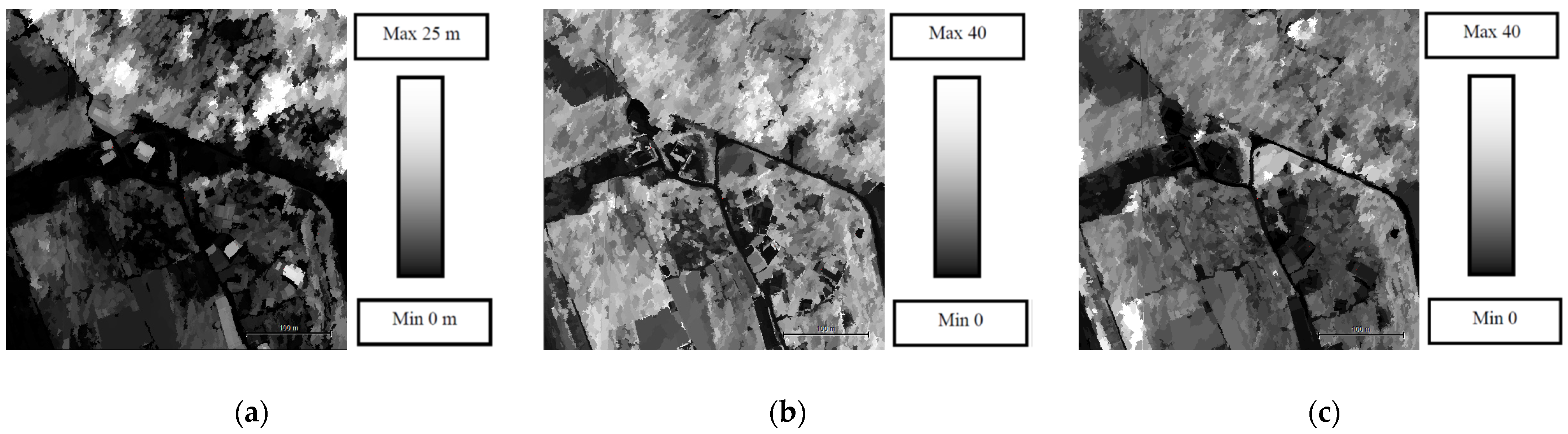
A C# program was written to extract the parameter values from the ASCII file of the LiDAR data, and then it was loaded into the image processing software for calculation. The research parameter LAS file can be obtained and loaded into the eCognition software for operation, and the image results of elevation difference, dispersion, and wave width can be obtained, respectively. As shown in
Figure 2. The closer the parameter image is to the white block image, the higher the value, and vice versa; the closer to the black block image, the lower the value.
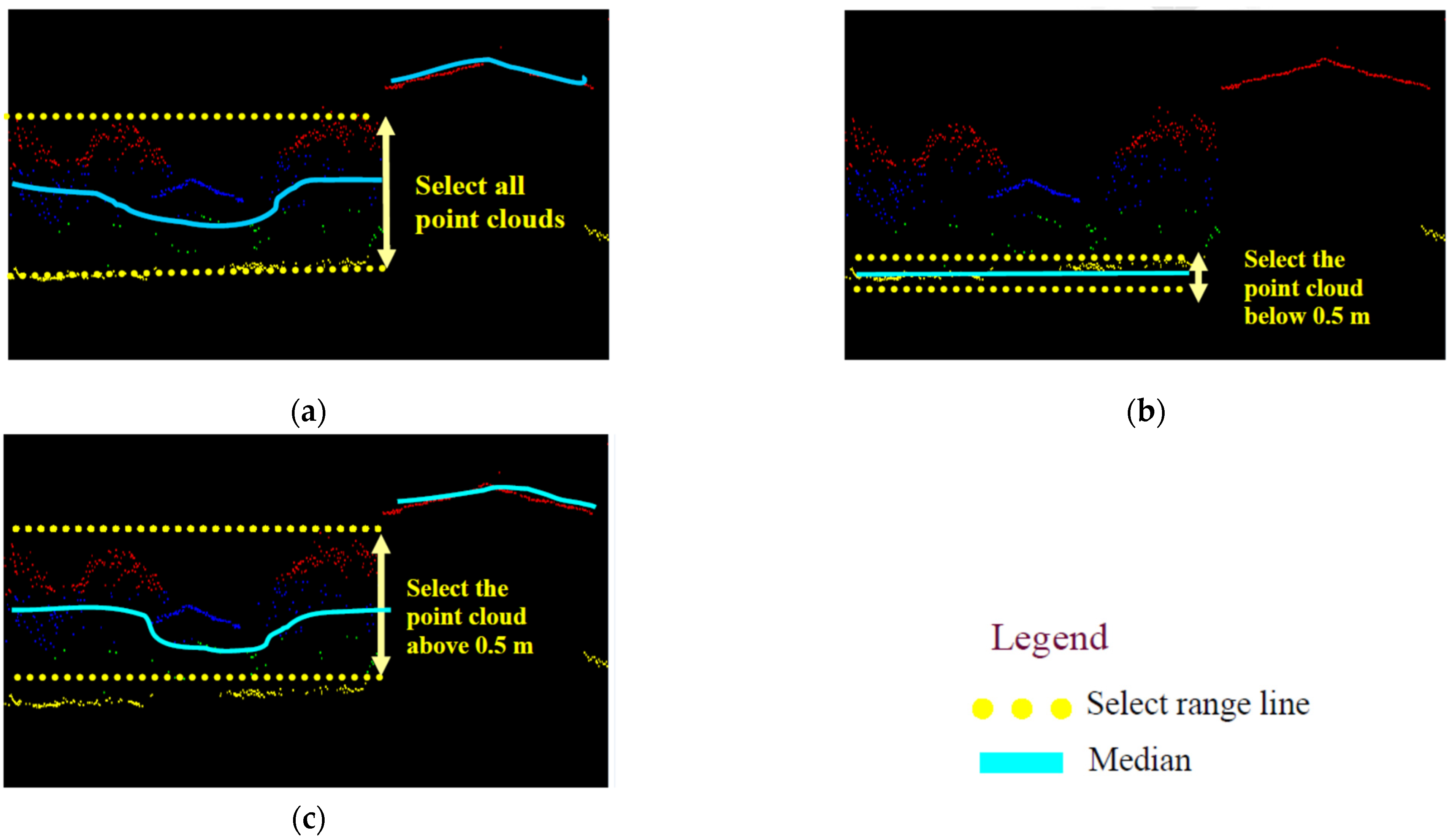
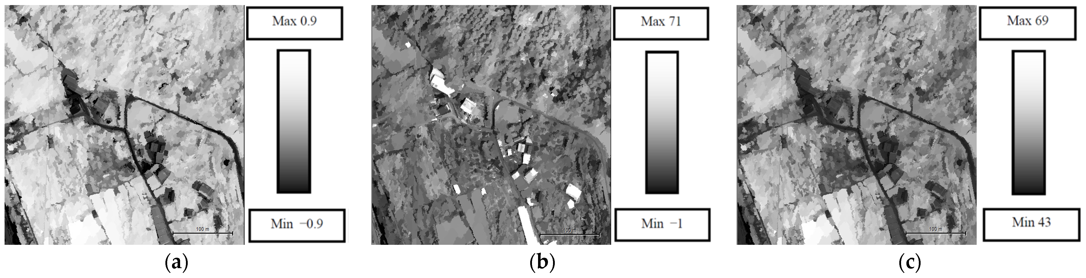
LiDAR data is point data in three-dimensional space. In order to understand the influence of elevation parameters on classification accuracy, this research will use the elevation difference of different objects according to the height characteristics of objects to be used as classification parameters. According to the actual observation of the objects in the study area, those with an elevation below 0.5 m are mainly artificial ground, bare land, and grassland, and those with an elevation above 0.5 m are mainly buildings, trees, and planted shrubs. In order to effectively separate the elevations of various types of objects to achieve the goal of the best classification, this research uses the above-mentioned observation data to customize the height value of the parameter. The self-defined elevation is divided into 3 parts, with 0.5 m as the boundary. The first part selects point cloud data of all elevations, as shown in
Figure 3a. The second part selects the point cloud data whose elevation is between 0–0.5 m and takes the median as the parameter value, and the point cloud data exceeding 0.5 m will not be calculated, as shown in
Figure 3b. In the third part, the point cloud data whose elevation is above 0.5 m is selected, and the median is taken as the parameter value, and the point cloud data below 0.5 m are not calculated, as shown in
Figure 3c. The geometric parameters extracted from the LiDAR data are used as classification parameters to improve the results of land cover classification.
2.2.2. Aerial Photographs
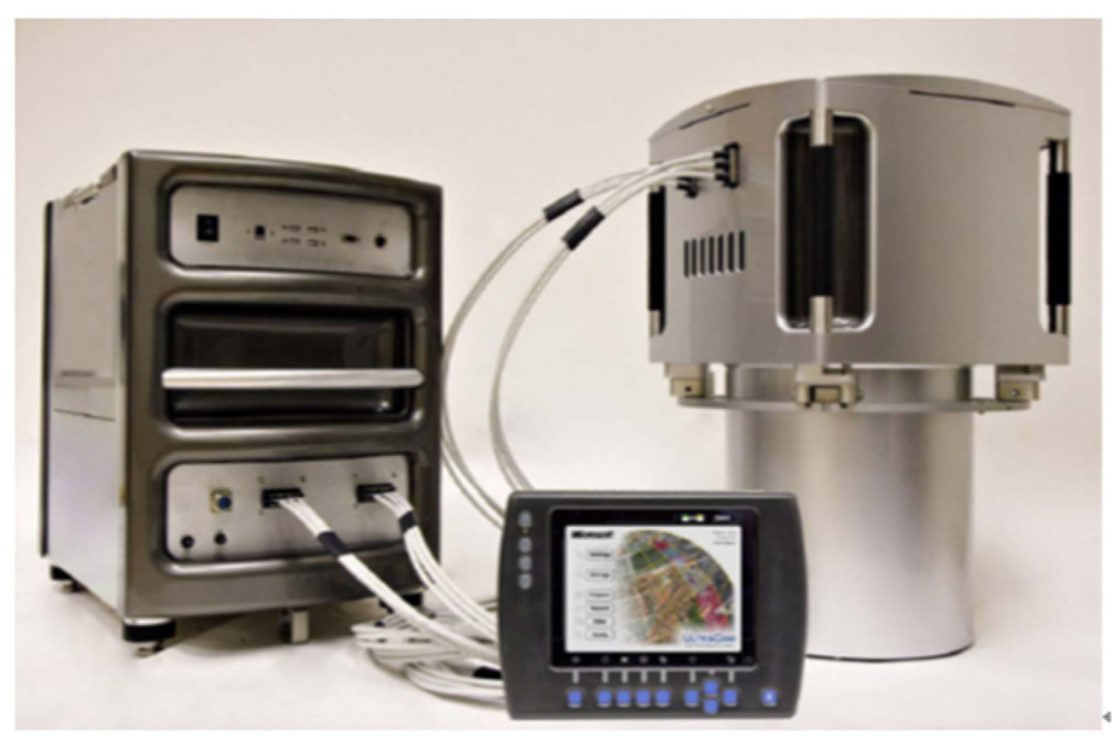
The collected aerial survey data can be divided into two categories: visible light images and near-infrared light images. The camera used is Microsoft Vexcel UltraCam-XP, and aerial photography is carried out in some mountainous areas in Taiping District, Taichung City, with an average altitude of 1700 m.
The camera was developed by Vexcel, as shown in
Figure 4, a subsidiary of Microsoft that specializes in spatial information. The system uses multi-lens in situ time-lapse exposure technology to achieve true central projection, which can solve the problem of image distortion of large format cameras. In terms of color capture capability, UltraCam-XP has the ability to receive R, G, B, and NIR four-band spectrum, and the color depth can reach 14 bits, which can present more saturated image details.
In this study, the NIR and Red bands in aerial photographs were used to calculate NDVI, Albedo, and SR values (collectively referred to as spectral parameters). The calculation equations are (1), (2), and (3), respectively. The principle is to use the characteristics that the more vigorous the growth of green plants, the more red light absorbed by chlorophyll, the stronger the reflection of infrared light, and the ratio of the two bands of near-infrared light and red light are combined into an indicator. The parameters selected in this study can effectively separate vegetation and non-vegetation features, and then the built-in feature definition function of eCognition software is used to calculate the value of feature parameters.
Figure 5 are the images presented by NDVI, Albedo, and SR values, respectively. In the image, the closer to the white block image, the higher the value, and vice versa; the closer to the black block image, the lower the value.
2.2.3. Image Classification Software
eCognition is an image classification software developed by German company Definiens Imaging, which can provide image users with automatic or semi-automatic image information extraction. It has been widely used in natural resources, environmental surveys, agriculture, forestry, and natural disaster monitoring. The advantage of its software is that, unlike traditional pixel-based classification methods, only image spectral values are used for image segmentation. Instead, the concept of object orientation is used, and the spectral characteristics and spatial characteristics of each pixel are referred to for image classification in the process of segmenting the original image into image objects. Adjacent pixels are merged into image objects one by one according to their homogeneity, the salt-and-pepper effect produced by traditional pixel-based classification methods is reduced, and the classification results are made more accurate.
In this study, the software will be used to classify the land cover of the study area, and the parameters obtained from airborne LiDAR and aerial photographs extraction will be imported into the software. In the selection process of the algorithm, factors such as the use of supervised classification methods in the literature on land cover classification using aerial telemetry images and the completion of the collection of land cover types to be classified in the study area were considered. Therefore, the DT classification method and the SVM classification method in its built-in supervised classification method are used as the classifiers of this study, and the classification results are compared with the ground truth data to verify their accuracy.
2.3. Land Cover Category
When applying remote sensing technology to land classification, the items of land categories are often defined according to the types of land cover or land use. According to different application purposes of users, the required land classification items are adopted. The classification systems that are often used to define the target categories of land feature classification include the United States Geological Survey (USGS) land cover classification system [
20], the European Union’s CORINE land cover classification system [
21], and the land resource utilization classification table in Taiwan. Items defined in each classification are not necessarily included in each region.
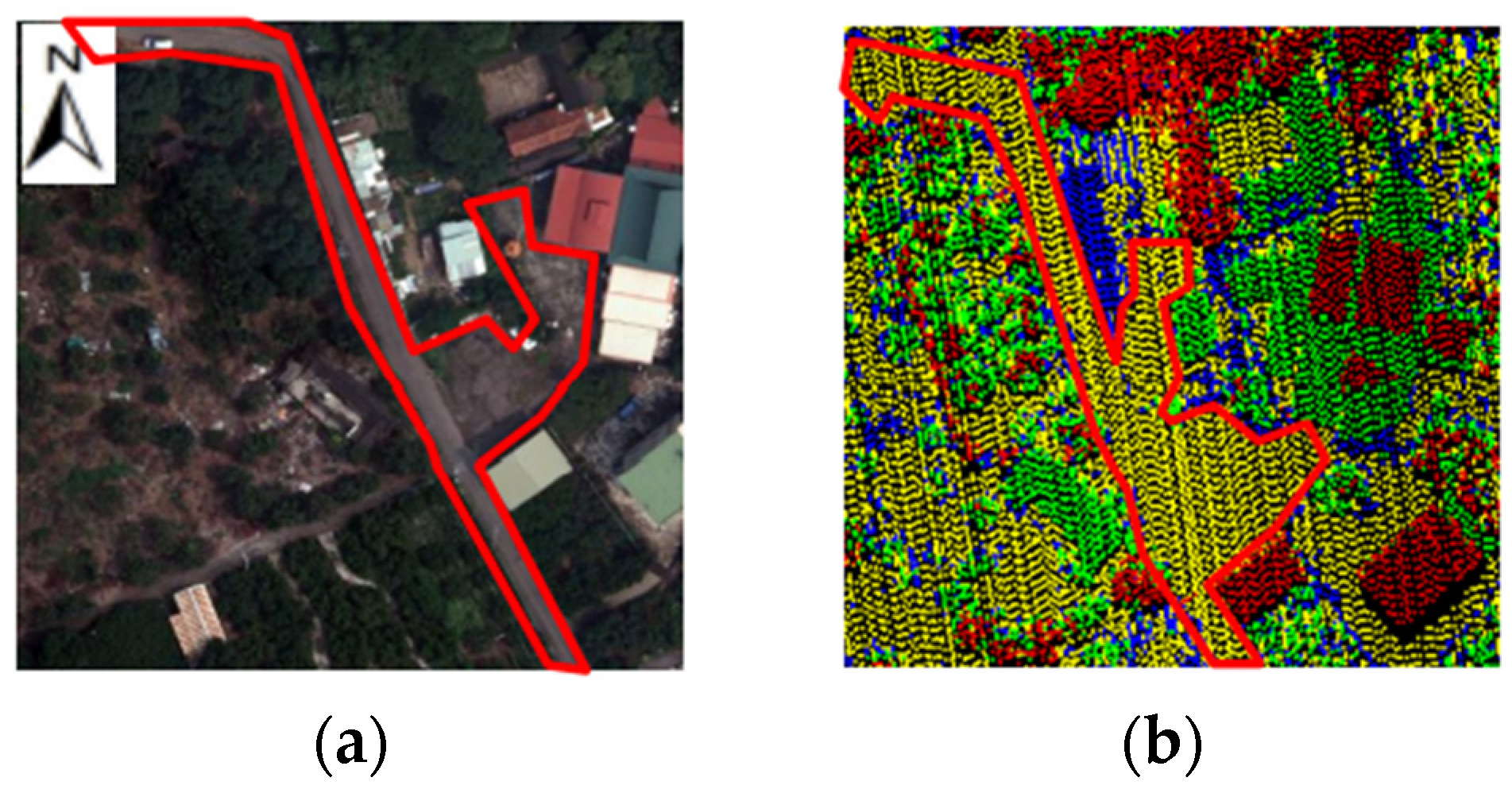
Therefore, this study refers to the above classification table and assigns appropriate classification categories to the land cover within the study area. Additionally, the existing parameters in the study area do not easily distinguish all types of trees. This study only classifies the starfruit trees, which are concentratedly planted by farmers in the study area, as shrubs, and other tree species as trees, and defines six land cover categories, including artificial surfaces, buildings, bare land, grassland, trees, and shrubs, based on the definition principles of the classification table, as shown in
Table 1. For example, artificial ground is defined as roads and concrete voids.
Figure 6 the area marked by the red range. Considering that the vacant land, industrial roads, and rural roads within the research scope have similar characteristics, they are all classified into one category.
2.4. Selection of Training Area and Ground Truth Data
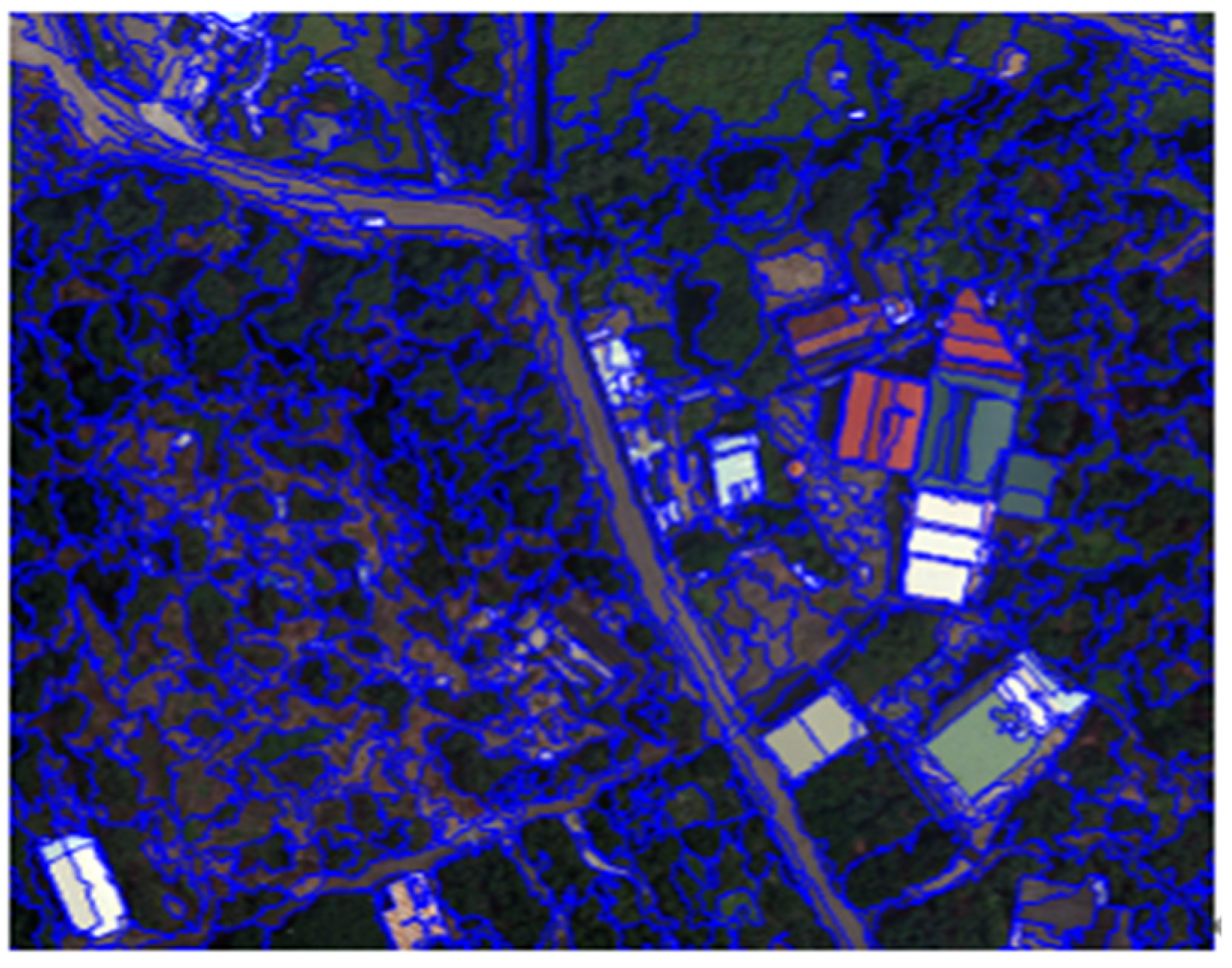
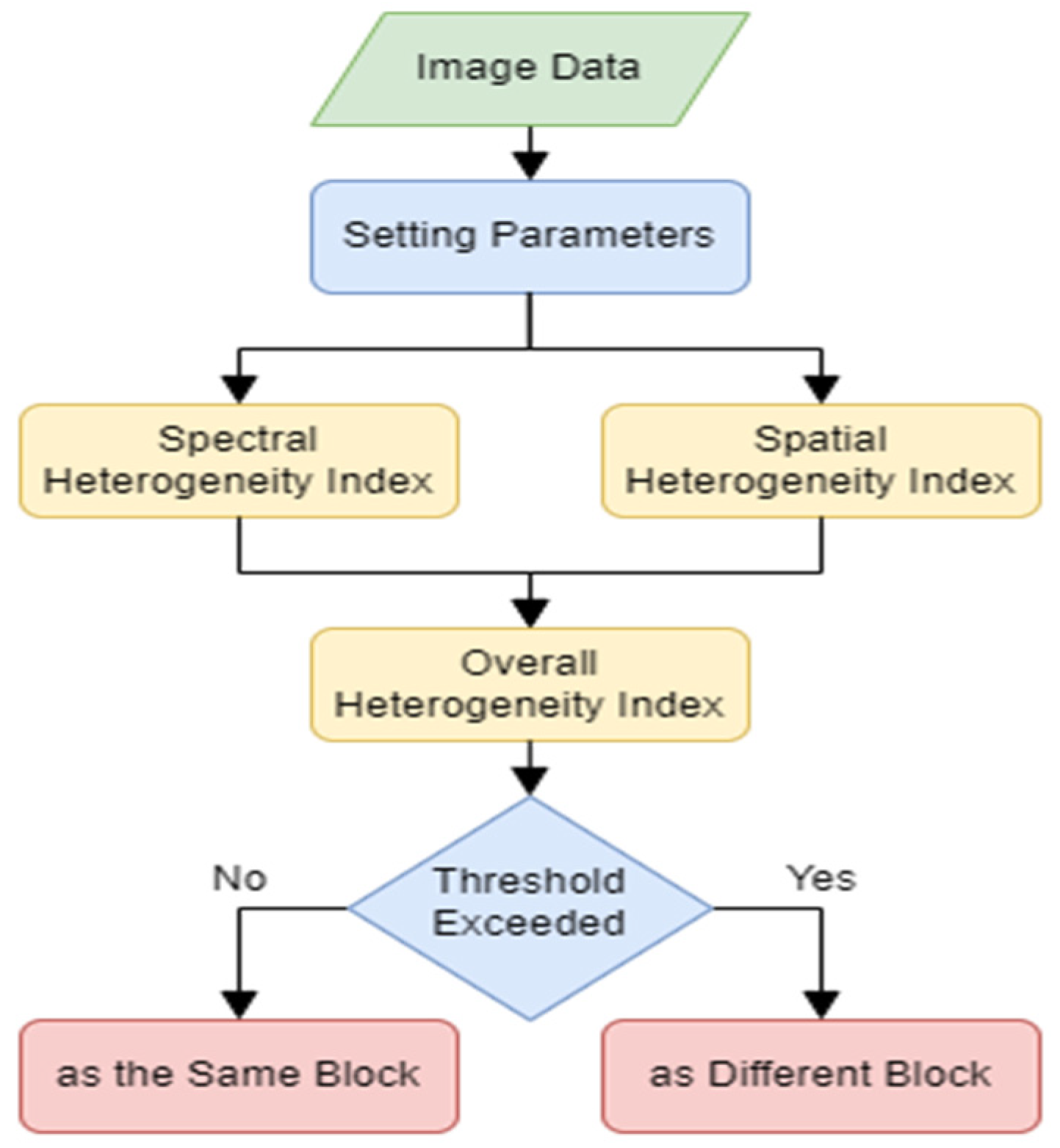
In this study, the multi-scale segmentation method built into the eCognition software was used for image segmentation processing. The heterogeneity index of each object in the image is calculated according to the image characteristics, and the threshold value of the heterogeneity index of the object is given to complete the goal of image segmentation. The concept of software operation is to first treat each pixel as a block on the basis of pixels, and then block merging is performed. Small blocks are aggregated into large blocks, and each time a small block is added, the heterogeneity index of the entire large block is calculated. If it is less than the threshold of heterogeneity, it is regarded as the same block, and if it exceeds the threshold of heterogeneity, it is regarded as a different block, which can effectively reduce the salt and pepper effect caused by the traditional pixel classification method. The image of the research area segmented in this study is shown in
Figure 7.
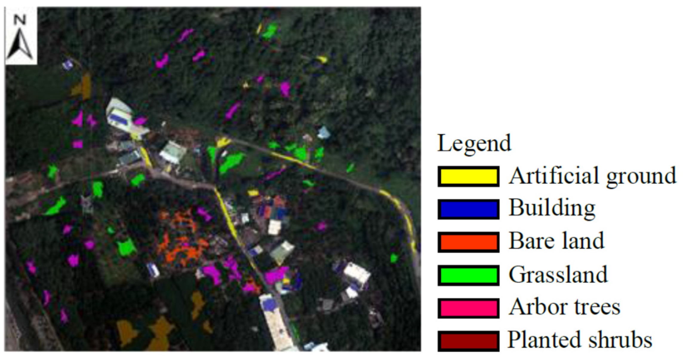
Six types of ground features, including artificial ground, buildings, bare land, grassland, arbor trees, and planted shrubs, were selected for sampling in the training area. Yellow stands for artificial ground, blue stands for buildings, orange stands for bare land, green stands for grassland, pink stands for arbor trees, and brown stands for planted shrubs. The training samples are shown in
Figure 8. Parameter values, such as the properties of different objects in each training area, can be observed through the built-in functions of the software, which can be divided into spectral images and geometric data, as shown in
Table 2 and
Table 3.
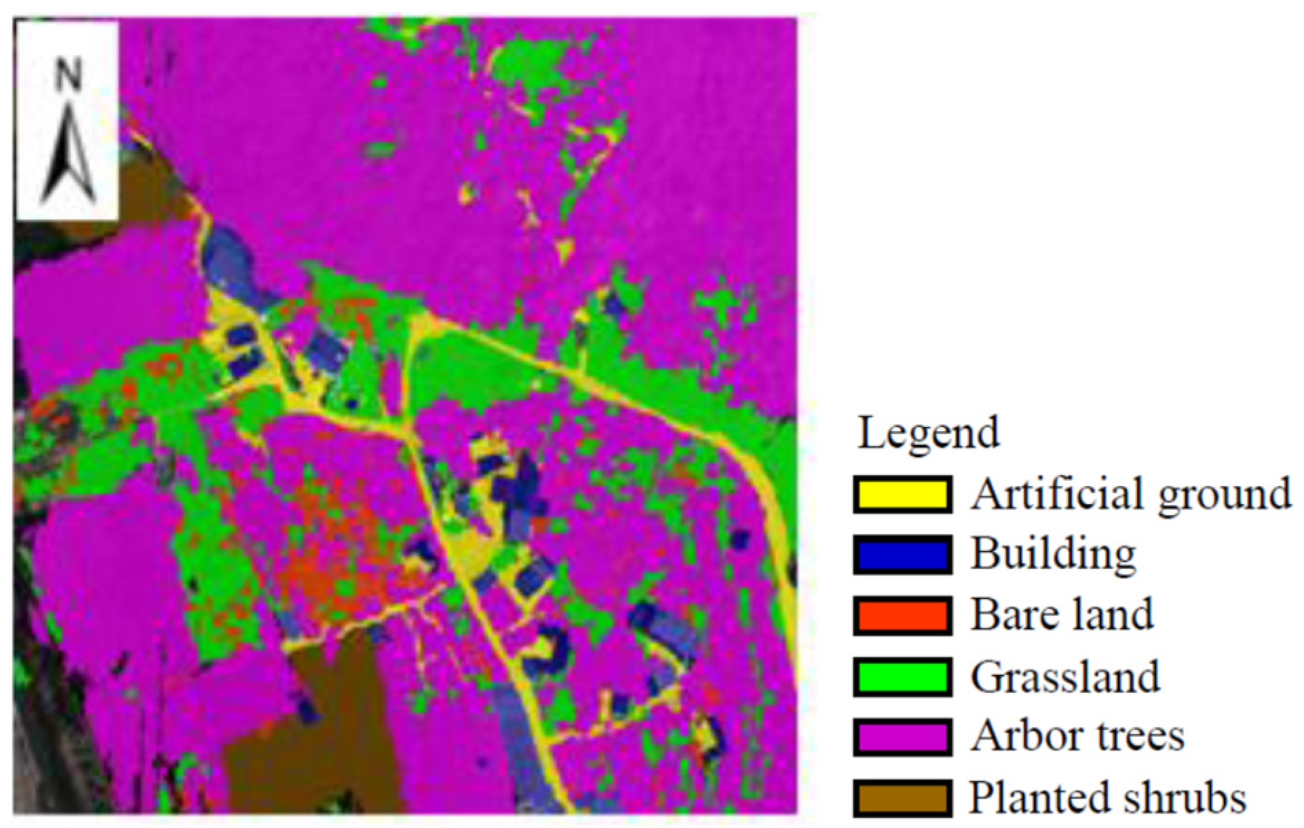
Ground truth data is the result of manual actual exploration and comparison of aerial photographs and LiDAR point cloud data. The land cover area in the study area is divided into six categories: artificial ground, buildings, bare land, grassland, arbor trees, and planted shrubs. Input the classified image as the true value and compile the true value attribute according to the built-in program setting of the image classification software. The image is shown in
Figure 9, and the statistics of the number of pixels are shown in
Table 4. In this study, due to the inconsistency between the LiDAR scanning data and the aerial photographs, the current conditions of some buildings and vegetation have dropped due to the time difference. In addition, because some private land surveys are not easy and there are scaffoldings on the grass that affect the point cloud elevation and image spectral values, there are still errors in the true value data, which affects the accuracy of the verification results.
2.5. Classification Methods
The image classification logic carried out by the object-oriented classification method is mainly to simulate and reconstruct the analysis and interpretation ability of the human eye. First, the image is segmented into reasonable blocks with different characteristics, and then the image objects are classified according to different index features, such as size, shape, organization, adjacency, and position. Compared with the traditional pixel-based classification method, the object-oriented classification method pays more attention to the topological relationship of space. The results are more accurate and representative when used in land cover classification.
The advantage of using the object-oriented classification method is that the spectral characteristics and spatial characteristics of each pixel are referred to in the process of segmenting the original image into image objects. Adjacent pixels are merged into image objects one by one according to their degree of homogeneity, and the image object is the result of quantizing the spatial characteristics into a homogeneous area, which can represent that the area has the same spatial characteristics. In image classification, in addition to spectral features, the homogeneity index in texture features is added to classify image objects, which can make the classification results more accurate.
Multiresolution Segmentation is an image segmentation method using Bottom-up Segmentation. The principle is to divide and process in the way of block growth, which is to merge smaller image objects, such as pixel data, to generate larger image objects. Alternatively, starting from the seed object, nearby candidate objects that meet the set threshold criteria are selected and combined into the same object target. Unlike traditional segmentation methods, shape factors can be added to help image segmentation, and different segmentation mechanisms can be set according to different image characteristics. In addition, by calculating the heterogeneity index of each object in the image and the threshold value of the heterogeneity index of a given object, the goal of image segmentation is achieved. The initial level is based on pixels, and each pixel is regarded as a block, and then the action of block merging is performed. Small blocks are aggregated into large blocks, and each time a small block is added, the heterogeneity index of the entire large block is calculated. If it is less than the threshold of heterogeneity, it will be regarded as the same block, and if it exceeds the threshold of heterogeneity, it will be regarded as different blocks. The operation process is shown in
Figure 10. When the threshold value is the same, images with relatively uniform land cover responses will generate larger blocks after image segmentation, which can effectively reduce the salt and pepper effect problems caused by traditional pixel-based classification methods [
22].
In [
23], IKONOS satellite image data was used to make a large-scale plant community classification map of the metropolitan area with the help of object-oriented classification method. Their results show that an object-oriented taxonomy can be applied to assess the biodiversity of vegetation in cities.
Two classification methods were used in this study: Decision Tree (DT) and Support Vector Machine (SVM), both of which are supervised classification methods. It does this by taking the training data (consisting of labeled samples of known classes) from a classification model and classifying it against the test data of unknown classes [
13].
For example, in [
24], using multiple echoes, full-waveform LiDAR, and multispectral image parameter data, the random forests classification method (RF) is used to classify urban objects.
DT is one of the commonly used classification functions in data mining processing technology. It can effectively handle classification prediction problems of categorical or continuous variables and produce clear multi-level classification decisions. The knowledge structure of this model is easy for users to understand, and the prediction accuracy is not worse than other methods [
25]. There are several advantages in the field of data mining that make it widely used:
The DT model can be represented by graphics or rules, and the intuitive representation makes the result rules of the classification model very efficient and easy to explain, understand, and use. Building a DT does not require the analyst to input any parameters;
When the training data set is sufficient, the correctness of the DT is not worse than other classification modes, and it is fast. When dealing with variables, it can also show the relative importance of model variables;
The algorithm of the DT is scalable. It can build a DT from a huge training database, and it can handle a large amount of data very well. When the amount of data is large, and many variables are input, the DT can still be constructed.
When building a DT, after a piece of data enters from the root node, the training test is used to select the appropriate node to enter the next layer. Although there are different algorithms for the selection of tests, the purpose is the same regardless of the algorithm. The testing process is repeated until the data reaches the leaf nodes. The construction process of DT usually includes the following three steps: select the DT algorithm, construct a DT from the training data set, and prune DT [
25].
SVM classification method originated from the machine learning system constructed using the theory of statistical learning [
26]. The main principle is to seek the hyperplane with the largest boundary in the feature space to distinguish different binary categories. SVM can be divided into linear and nonlinear. If the distribution of training samples in the space is nonlinear, nonlinear SVM is adopted; otherwise, linear SVM is adopted. Linear SVM can be further classified as linearly separable or linearly inseparable.
SVM realizes the consistency of the learning process and the principle of structural risk minimization. By comprehensively considering the empirical risk and the credible interval and taking a compromise according to the principle of structural risk minimization, the decision function with the smallest risk is obtained. Its core idea is to map the samples of the input space to the high-dimensional kernel space with nonlinear changes and obtain the optimal linear decision surface with low complexity in the high-dimensional kernel space. The main purpose of classification is to find a hyperplane for a group of data in the feature space and divide this group of data into two groups (Group A and Group B) via the hyperplane. The data belonging to Group A are located on the same side of the hyperplane, while the data of Group B are located on the other side of the hyper-plane. In order to clearly distinguish Groups A and B, the larger the margin between the two groups, the better the separation. Generally, the functions that can be divided linearly have formulas such as (4). When dealing with non-linear data, the linear function cannot be separated, and the attribute transposition must be carried out to transfer the data to a higher-dimensional space or feature space in order to distinguish them. The formulas are as follows (5). Usually, the conversion function is a complex function that is not easy to obtain, so the inner product of the conversion function is used to obtain a simpler function, which is called a kernel function [
27,
28].
Nonlinear attribute transformation
:
The basic classification principle of SVM is based on binary categories. Therefore, the multi-category classification method can expand from two to multiple categories through one-against-all or one-against-one method. In this study, one-against-all method is used, assuming that there are N categories of samples, and N classifiers will be generated by one-to-many classification; that is, a classifier will be generated between each category and the remaining categories. Finally, the SVM with the largest classification function is used as the category of the sample to be classified. This classification method is also often used in the full-waveform LiDAR land cover classification [
29].
2.6. Accuracy Evaluation
In this study, the error matrix is used to evaluate the accuracy of the classification results [
30]. Through the matrix, the corresponding relationship between the classification results and the inspection data can be displayed. This study first uses the error matrix to display the results of land cover classification and compares and verifies the results of land cover classification with the manually drawn ground truth data to evaluate the accuracy of the classification results.
Using the error matrix method and ground truth data to verify the quality of the classified data, the User’s Accuracy (UA) of the ground truth data, the object-oriented DT classification method, and the Producer’s Accuracy (PA) generated by the object-oriented SVM classification method are, respectively, used; and Overall Accuracy (OA) is used to further verify the research results.
3. Results and Discussion
3.1. Phase 1 Experiment: Classification with LiDAR Data and DT
Phase 1 experiment: We mainly used the elevation difference, dispersion, and wave width extracted from LiDAR data as characteristic parameters and divided the parameter-defined elevation into three categories. The first type of parameter is to select the entire point cloud range as the feature basis. The second type of parameter is to select the point cloud range below 0.5 m as the feature basis. The third type of parameter is to select the point cloud range above 0.5 m as the feature basis. According to the combination of different characteristics, it is divided into five groups, as shown in
Table 5.
3.1.1. Phase 1 Classification Results
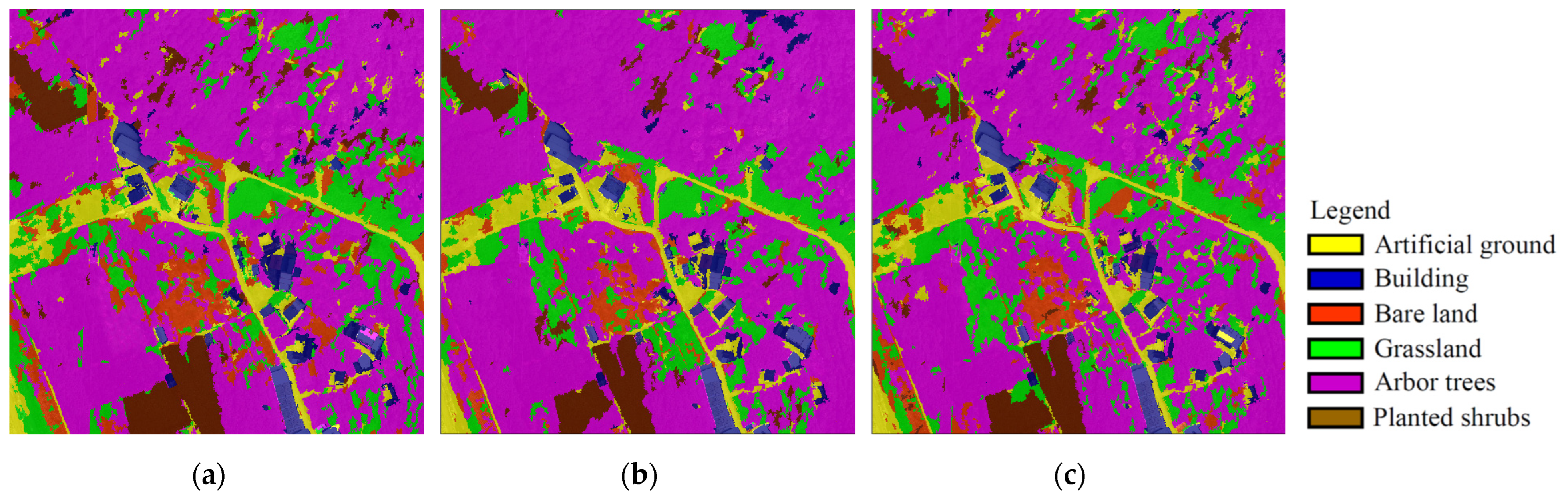
Group 1: The parameters of elevation difference, dispersion, and wave width extracted from the airborne LiDAR data were input into the eCognition image classification software, and the DT method was used to classify the land cover. The classification results are shown in
Figure 11a. The OA is 59%, and the Kappa value is 38%. Comparing the accuracy of each land cover category, the PA is the highest at 89% for the arbor category and the lowest for the bare land category at 22%; the UA is the highest at 96% for the building category and the lowest at 40% for the bare land category.
Group 2: The parameters of elevation difference, dispersion, and wave width were extracted from the airborne LiDAR data, and the parameter elevation was customized with 0.5 m as the dividing line. The eCognition image classification software was input, respectively, and the DT method was used to classify the land cover. The classification results are shown in
Figure 11b. The OA is 59%, and the Kappa value is 32%. Comparing the accuracy of each land cover category, the PA is the highest at 83% for planting shrubs and the lowest at 21% for grasslands. The UA is highest at 82% for buildings and the lowest at 31% for grasslands.
Group 3: The parameters of elevation difference, dispersion, and wave width were extracted from the airborne LiDAR data, the parameters were customized with the elevation of 2.5 m as the dividing line, they were input into the eCognition image classification software, and the DT method was used to classify land cover. The classification results are shown in
Figure 11c. The OA is 65%, and the Kappa value is 45%. Comparing the accuracy of each land cover category, the PA is the highest at 92% for the arbor type and the lowest for the grassland type at 33%; the UA is the highest for the planted shrub type at 81% and the lowest for the bare land type at 30%.
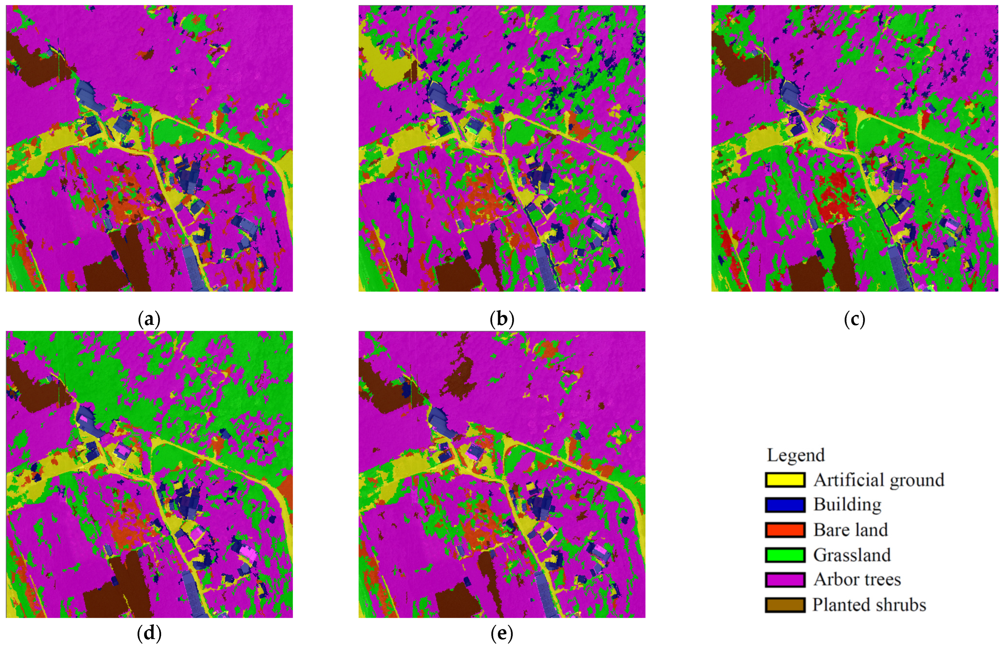
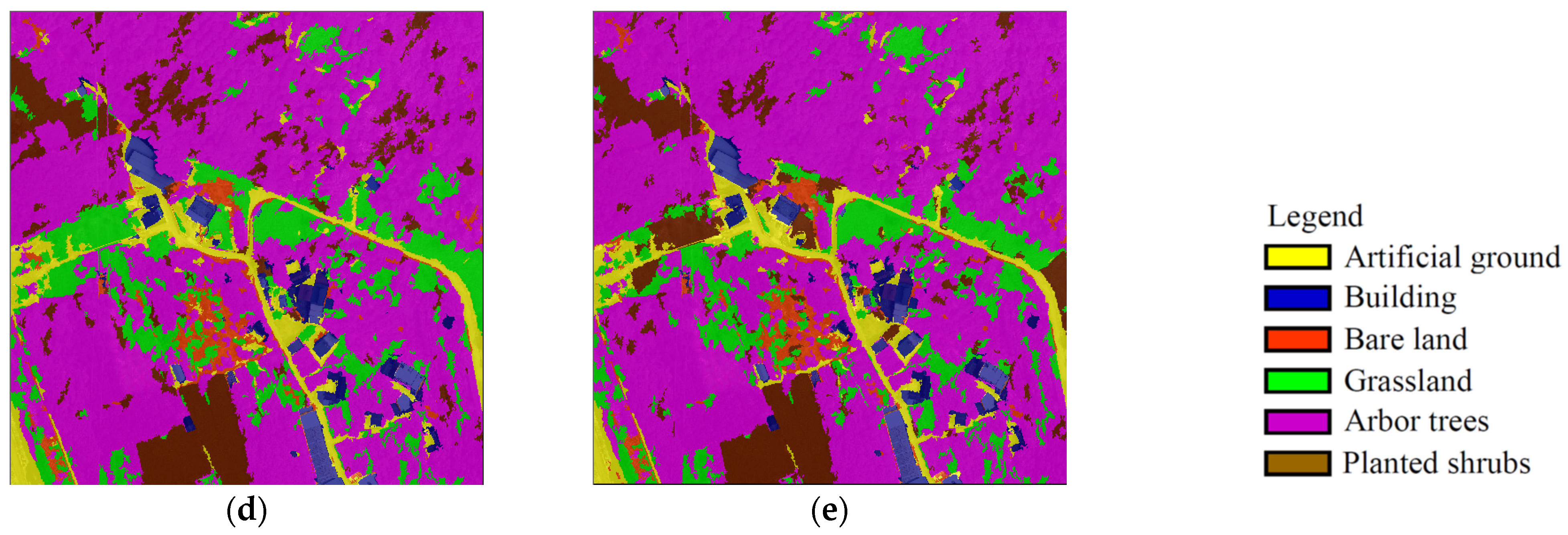
Group 4: The original values of the parameter’s elevation difference, dispersion, and wave width were extracted from the airborne LiDAR data, and the parameters of the self-defined elevation with 0.5 m were customized as the dividing line. The eCognition image classification software was input, respectively, and the DT method was used for land cover classification. The classification results are shown in
Figure 11d. The OA is 63%, and the Kappa value is 43%. Comparing the accuracy of each land cover category, the PA was the highest at 92% for planting shrubs and the lowest at 26% for grassland. The UA is the highest at 97% for planted shrubs and the lowest at 38% for bare land.
Group 5: The original values of the parameter’s elevation difference, dispersion, and wave width were extracted from the airborne LiDAR data, and the parameters of the self-defined elevation with 2.5 m were customized as the dividing line. The eCognition image classification software was input, respectively, and the DT method was used for land cover classification. The classification results are shown in
Figure 11e. The OA is 82%, and the Kappa value is 67%. Comparing the accuracy of each land cover category, the PA was the highest at 92% for planted shrubs and the lowest for bare land at 31%. The UA is highest at 92% for trees and 37% for bare land.
3.1.2. Phase 1 Discussion
The group parameter results of Phase 1 experiment are shown in
Table 6. The classification results of Groups 1 to 3 are compared. The parameters of Group 1 using LiDAR data (all point cloud range) and Group 2 using LiDAR data (point cloud range below 0.5 m) have an OA of 59%, with no significant difference. However, the third group uses the parameters of LiDAR data (point cloud range above 0.5 m), and its OA increased to 65%. Among them, the accuracy of trees and grasslands is more obvious, and the other categories are less obvious. In summary, using the parameters of LiDAR data (point cloud range above 0.5 m) can effectively improve the accuracy of classification results.
Comparing the classification results of Groups 4 and 5, Group 4 also uses the parameters of LiDAR data (the entire point cloud range and the point cloud range below 0.5 m), and the OA is 63%. However, the fifth group used the parameters of LiDAR data (all point cloud range and point cloud range above 0.5 m), and its OA increased to 82%. It can be seen that using the entire point cloud range and the LiDAR data parameters of the point cloud range above 0.5 m can effectively improve the performance of the OA.
The classification results of Groups 1 to 5 are compared. The PA and UA of the 3 types of trees, buildings, and planted shrubs are in the range of 43% to 97%. The PA and UA of artificial ground, grassland, and bare ground are in the range of 20% to 72%. It is judged that the reason is that the characteristics of the three types of trees, such as trees, are quite different in terms of spectrum, elevation difference, dispersion, and wave width. Compared with the artificial ground and the other three types, the difference in characteristics is less obvious, so it is easy to misjudge the classification, resulting in poor classification results.
3.2. Phase 2 Experiment: Classification with LiDAR Data, Aerial Photographs, and DT
Phase 2 Experiment: Spectral parameters extracted from aerial photographs, such as NDVI, Albedo, SR, and geometric parameters with better classification results of LiDAR data in the first stage experiment are mainly used, and they are imported into image classification software for land cover classification research. The land cover is divided into six categories: artificial ground, buildings, bare land, grassland, trees, and shrubs. According to different characteristics, they are combined and divided into five groups, as shown in
Table 7.
3.2.1. Phase 2 Classification Results
Group 6: The parameters of NDVI, Albedo, and SR are extracted from the aerial photographs data and input into the eCognition image classification software, and the DT method is used to classify the land cover. The classification results are shown in
Figure 12a. The OA is 47%, and the Kappa value is 28%. Comparing the accuracy of each land cover category, the PA is the highest at 98% for the building category and 25% for the grassland category. The UA is the highest at 76% for artificial ground and 38% for trees.
Group 7: The parameters of NDVI, Albedo, and SR and the elevation difference parameters of Group 1 are extracted from the aerial photographs data and input into the eCognition image classification software, respectively, and the DT method is used for land cover classification. The classification results are shown in
Figure 12b. The OA is 78%, and the Kappa value is 63%. Comparing the precision of each land cover category, the producer precision was the highest at 92% for the arbor category and the lowest for the grassland category at 49%. The UA is highest at 87% for buildings and 37% for bare land.
Group 8: The parameters of NDVI, Albedo, and SR, as well as the parameters of elevation difference, dispersion, and wave width of Group 1, are extracted from the aerial photographs data and were, respectively, input into the eCognition image classification software, and the DT method is used for land cover classification. The classification results are shown in
Figure 12c. The OA is 79%, and the Kappa value is 65%. Comparing the precision of each land cover category, the producer precision is the highest at 91% for the arbor category and the lowest at 50% for the grassland category. The UA is highest at 96% for buildings and 43% for bare land.
Group 9: The parameters of NDVI, Albedo, and SR, and the elevation difference, dispersion, and wave width of Group 4 are extracted from the aerial photographs data and input into the eCognition image classification software, and the DT method is used for land cover classification. The classification results are shown in
Figure 12d. The OA is 83%, and the Kappa value is 70%. Comparing the accuracy of each land cover category, the PA is the highest at 91% for trees and 47% for planted shrubs. The UA is highest at 97% for buildings and 42% for bare land.
Group 10: The parameters of NDVI, Albedo, and SR, as well as the elevation difference, dispersion, and wave width of Group 5, are extracted from the aerial photographs data and input into the eCognition image classification software, and the DT method is used for land cover classification. The classification results are shown in
Figure 12e. The OA is 84%, and the Kappa value is 72%. Comparing the accuracy of each land cover category, the PA is the highest at 93% for trees and 44% for planted shrubs. The UA is highest at 96% for buildings and 45% for bare land.
3.2.2. Phase 2 Discussion
The group parameter results of Phase 2 experiment are shown in
Table 8. The classification results of Groups 6 and 7 are compared. Group 6 used spectral parameters from aerial photographs, and its OA was 47%. Group 7 used aerial photographs and added the elevation difference parameters of LiDAR data, and its OA increased to 78%. The classification results of each category have improved, among which the accuracy of trees and planted shrubs have been improved more significantly, and the other categories are less obvious. In summary, using the elevation difference parameters of LiDAR data can effectively improve the accuracy of classification results, especially in improving the classification results of trees and planted shrubs.
Compare the classification results of Groups 6 and 8. Group 6 used spectral parameters from aerial photographs, and its OA was 47%. In the eighth group, the elevation difference, dispersion, and wave width parameters of the LiDAR data are added, and the OA is increased to 79%. The classification results of each category have improved, and the same as the results of the seventh group, the accuracy of the improvement of trees and shrubs is more obvious. To sum up, it can be seen that using aerial photographs and LiDAR data as classification parameters can effectively improve OA.
The classification results by Groups 9 and 10 are compared. Group 9 used the parameters of aerial photographs and LiDAR data (all point cloud ranges and point cloud ranges below 0.5 m), and its OA was 83%. Group 10 used the parameters of aerial photographs and LiDAR data (all point cloud ranges and point cloud ranges above 0.5 m), and its OA was 84%. It can be seen from this that when the classification accuracy reaches a certain level, the effect of using self-defined elevation parameters to improve the classification accuracy is also limited.
The classification results of Groups 6 to 10 are compared. The PA and UA of trees, buildings, and planted shrubs are in the range of 44–93%. The PA and UA of artificial ground, grassland, and bare ground are in the range of 37–81%. The results are the same as those of the first stage experiment. It can be seen that the aerial photographs and LiDAR data used in this study have higher classification results for trees, buildings, and planted shrubs than artificial ground, grassland, and bare land.
3.3. Phase 3 Experiment: Classification with LiDAR Data, Aerial Photographs, and SVM
Phase 3 Experiment: The parameters of the better group of classification results in the first and second stage experiments were mainly extracted and divided into three groups according to different feature combinations, as shown in
Table 9. The parameters were reclassified with the SVM method to verify the land cover of the study area. If the algorithm is changed from the DT method to the SVM method, will the accuracy of the classification results be improved.
3.3.1. Phase 3 Classification Results
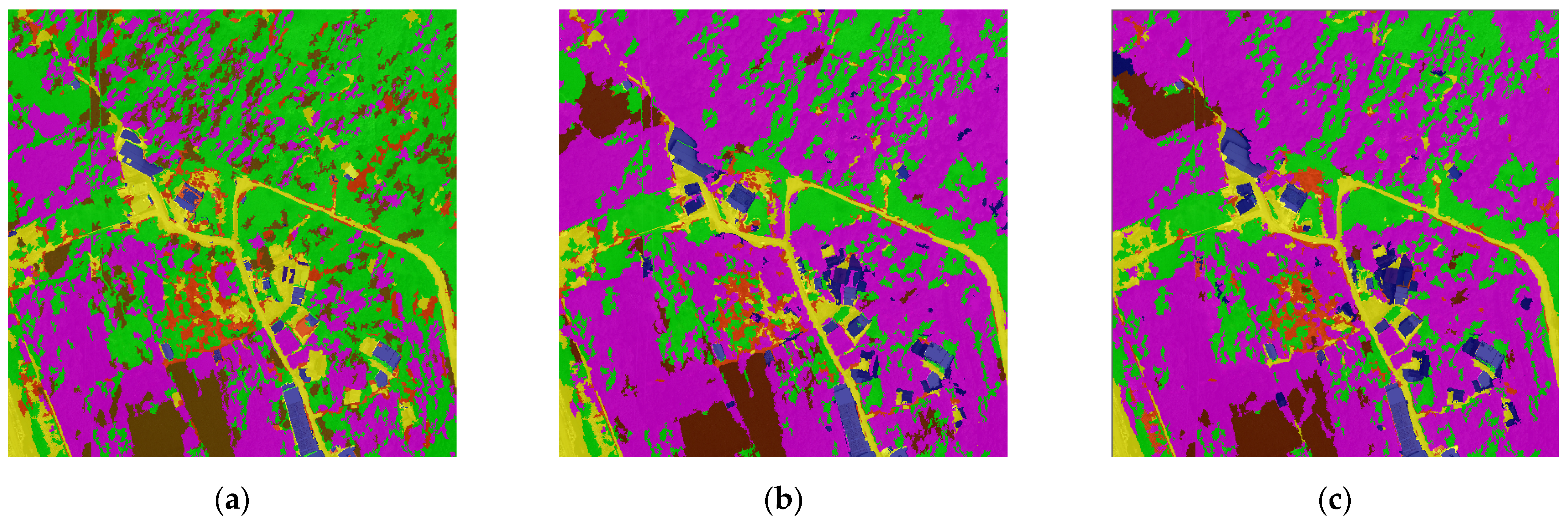
Group 11: The elevation difference, dispersion, wave width, and other self-defined parameters of Group 5 were extracted from the airborne LiDAR data and input into the eCognition image classification software, respectively, and the SVM method was used to classify the land cover. The classification results are shown in
Figure 13a. The OA is 79%, and the Kappa value is 64%. Comparing the precision of each land cover category, the producer precision is the highest at 94% for the arbor category and 26% for the bare land category. The UA is highest at 96% for buildings and 51% for grasslands.
Group 12: From aerial Photographs and airborne LiDAR data, self-defined elevation parameters such as elevation difference, dispersion, and wave width in Group 1 and NDVI, Albedo, and SR parameters in Group 6 are extracted. The eCognition image classification software was input, respectively, and the SVM method was used to classify the land cover. The classification results are shown in
Figure 13b. The OA is 79%, and the Kappa value is 64%. Comparing the precision of each land cover category, the producer precision is the highest at 92% for the arbor category and 57% for the bare land category. The UA is highest at 94% for buildings and 54% for bare land.
Group 13: From aerial photographs and airborne LiDAR data, self-defined elevation parameters such as elevation difference, dispersion, and wave width in Group 5 and NDVI, Albedo, and SR parameters in Group 6 are extracted. The eCognition image classification software are input, respectively, and the SVM method are used to classify the land cover. The classification results are shown in
Figure 13c. The OA is 80%, and the Kappa value is 65%. Comparing the accuracy of each land cover category, the PA is the highest at 92% for the arbor category and the lowest for the grassland category at 35%. The UA is highest at 89% for buildings and 54% for bare land.
3.3.2. Phase 3 Discussion
The group parameter results of Phase 3 experiment are shown in
Table 10. Group 11 used LiDAR data and the SVM method, and its OA was 78%. Compared with the accuracy of the DT method under the same parameters in the first group of experiments was 82%, the OA is about 4% lower.
The results of Groups 5 and 11 are compared. Group 11 used aerial photographs, LiDAR data and SVM method, and its OA was 78%, compared with the 82% accuracy of the DT method in Group 5 under the same parameters. In the comparison of the classification results of various types of land cover, the classification results of Group 5 in trees and grasslands are better. Group 11 has better classification results in planted shrubs, bare ground, and artificial ground. The accuracy of the two results is similar for the building-in-progress category.
The results of Groups 8 and 12 are compared. Group 12 used aerial photographs, LiDAR data, and the SVM method, and its OA was 84%, compared with the 79% accuracy of the DT method in Group 8 under the same parameters. In the comparison of the classification results of various types of land cover, the classification results of Group 8 under construction, planted shrubs, and artificial ground are better. Group 12 has better classification results in trees, grasslands, and bare lands.
The results of Groups 10 and 13 are compared. Group 13 uses aerial photographs, LiDAR data, SVM method, and its OA is 80%, compared with the 84% accuracy of the DT method in Group 10 under the same parameters. In terms of the classification results of various types of land cover, Group 10 has better results in the classification of grassland, buildings, bare land, and artificial ground. Group 13 achieved better results in the classification of planted shrubs. In the arbor category, the accuracy of both results is similar.
Based on the above accuracy, both the DT method and the SVM method have advantages and disadvantages in land cover classification results, and it is impossible to prove which algorithm has obvious advantages. In the follow-up, other parameters should be added, or the user should consider which land cover classification results (such as trees and grassland) are the priority objects to be judged and then select the required algorithm.
4. Conclusions
Based on this research, the following conclusions can be summarized.
(1) In this study, customized elevations extracted from LiDAR data were used as classification parameters. When selecting point cloud ranges below 0.5 m as classification parameters, the classification results were consistent with using the entire point cloud range, with an overall accuracy of 59%. However, when selecting point cloud ranges above 0.5 m, classification parameters resulted in an overall accuracy of 65%, which is a 6% improvement. This indicates that setting appropriate elevation parameters for LiDAR data can improve overall accuracy in land classification.
(2) When only using NDVI, Albedo, and SR from aerial images as classification parameters, the overall accuracy was 47%. However, if the elevation difference parameter from LiDAR data was added, the overall accuracy could be improved to 78%. This demonstrates that using elevation difference as a classification parameter plays an important role in assisting with land interpretation and can effectively improve overall accuracy.
(3) In this study, aerial images and LiDAR data were used, and DT and SVM algorithms were employed for land classification. The highest overall accuracy achieved was 84%. This indicates that the relevant parameters and classification methods selected in this study have achieved good classification results and can be effectively applied to land recognition tasks.
(4) This study found that image classification software is prone to segmentation deviations when dealing with objects of similar colors but different types, leading to errors in land segmentation. This is particularly true when dealing with objects that are connected and have similar elevation values, which can lead to a decrease in accuracy in subsequent land classification and verification operations. Therefore, when conducting land segmentation and verification operations, consideration should be given to whether similar objects should be used as training area samples and included in ground truth data comparisons to avoid affecting classification accuracy.
(5) Comparing the classification results of various experimental groups, the producer and user accuracies for tree, building, and shrub categories ranged from 43% to 97%, while the producer and user accuracies for artificial ground, grass, and bare soil categories ranged from 20% to 72%. It was judged that this is because the differences in spectral, elevation difference, dispersion, and bandwidth characteristics of tree, building, and shrub categories are relatively large, while the differences in characteristics for artificial ground, grass, and bare soil categories are less obvious, making it easier to misclassify these objects and resulting in poor classification results.
Based on this research, we suggest the following.
(1) This study only extracted six different parameter values from aerial imagery and airborne LiDAR data as the basis for land cover classification. It is recommended to add relevant parameter categories such as hyperspectral bands and amplitude in the future to effectively differentiate between various land cover categories, improve classification accuracy, and increase the number of classifiable land cover categories.
(2) Using object-oriented classification software as a tool for land cover classification can indeed provide good classification results. It is recommended to use its built-in classification algorithms (such as DT, SVM, and RF) to compare land cover classifications in different areas (such as urban, coastal, or mountainous areas) in order to find the correlation between applicable classification algorithms and areas.
(3) This study utilized eCognition object-oriented classification software, which not only allowed the incorporation of parameters for land cover classification but also enabled adjustments to the color and shape of objects within the study area that could be merged based on homogeneity indices and other features. It is recommended that future studies further explore the built-in features of software, such as homogeneity indices, to identify suitable indicator values for differentiating various ground objects, thus improving the accuracy of land cover classification.
(4) This study did not verify and compare the results with other study areas. It is recommended to use aerial imagery and airborne LiDAR data from different time periods and flying heights to conduct land cover classification research, compare parameter differences between different flight strips, and analyze and identify universally applicable classification parameter data to improve the practicality of relevant parameters.
Author Contributions
Conceptualization, M.-D.T. and C.-C.L.; Data curation, K.-W.T. and C.-T.W.; Formal analysis, K.-W.T.; Funding acquisition, M.-D.T.; Investigation, C.-C.L.; Methodology, M.-D.T. and C.-C.L.; Project administration, M.-D.T. and C.-T.W.; Resources, M.-D.T.; Software, M.-D.T.; Supervision, M.-D.T. and K.-F.C.; Validation, K.-W.T. and C.-T.W.; Visualization, K.-W.T. and C.-T.W.; Writing—original draft, C.-C.L.; Writing—review and editing, K.-W.T. and C.-T.W. All authors have read and agreed to the published version of the manuscript.
Funding
This research received no external funding.
Data Availability Statement
The data presented in this study are available on request from the corresponding author.
Acknowledgments
The authors thank Strong Engineering Consulting Co., Ltd. for assisting in LiDAR data collection and data preprocessing and other related technical support operations.
Conflicts of Interest
The authors declare no conflict of interest.
References
- Diaz, J.C.F. Lifting the Canopy Veil Airborne LiDAR for Archeology of Forested Areas. Imaging Notes Mag. 2011, 26, 31–34. [Google Scholar]
- Mallet, C.; Bretar, F. Full-waveform topographic LiDAR: State-of-the-art. ISPRS J. Photogramm. Remote Sens. 2009, 64, 1–16. [Google Scholar] [CrossRef]
- Chen, Z.; Gao, B.; Devereux, B. State-of-the-Art: DTM Generation Using Airborne LIDAR Data. Sensors 2017, 17, 150. [Google Scholar] [CrossRef] [PubMed]
- Kong, D.; Xu, L.; Li, X.; Li, S. A real-time method for DSM generation from airborne LiDAR data. In Proceedings of the 2013 IEEE International Instrumentation and Measurement Technology Conference (I2MTC), Minneapolis, MN, USA, 6–9 May 2013; pp. 377–380. [Google Scholar] [CrossRef]
- Doneus, M.; Briese, C.; Fera, M.; Janner, M. Archaeological prospection of forested areas using full-waveform airborne laser scanning. J. Archaeol. Sci. 2008, 35, 882–893. [Google Scholar] [CrossRef]
- Zhu, L.; Hyyppä, J. Fully-Automated Power Line Extraction from Airborne Laser Scanning Point Clouds in Forest Areas. Remote Sens. 2014, 6, 11267–11282. [Google Scholar] [CrossRef]
- Jovanović, D.; Milovanov, S.; Ruskovski, I.; Govedarica, M.; Sladić, D.; Radulović, A.; Pajić, V. Building Virtual 3D City Model for Smart Cities Applications: A Case Study on Campus Area of the University of Novi Sad. ISPRS Int. J. Geo-Inf. 2020, 9, 476. [Google Scholar] [CrossRef]
- Boguszewski, A.; Batorski, D.; Ziemba-Jankowska, N.; Dziedzic, T.; Zambrzycka, A. LandCover.ai: Dataset for Automatic Mapping of Buildings, Woodlands, Water and Roads from Aerial Imagery. In Proceedings of the IEEE/CVF Conference on Computer Vision and Pattern Recognition (CVPR) Workshops, Nashville, TN, USA, 19–25 June 2021; pp. 1102–1110. [Google Scholar]
- Zhang, W.; Gao, F.; Jiang, N.; Zhang, C.; Zhang, Y. High-Temporal-Resolution Forest Growth Monitoring Based on Segmented 3D Canopy Surface from UAV Aerial Photogrammetry. Drones 2022, 6, 158. [Google Scholar] [CrossRef]
- Zhang, Y.; Wu, H.; Yang, W. Forests Growth Monitoring Based on Tree Canopy 3D Reconstruction Using UAV Aerial Photogrammetry. Forests 2019, 10, 1052. [Google Scholar] [CrossRef]
- Bożek, P.; Janus, J.; Mitka, B. Analysis of Changes in Forest Structure using Point Clouds from Historical Aerial Photographs. Remote Sens. 2019, 11, 2259. [Google Scholar] [CrossRef]
- Adade, R.; Aibinu, A.M.; Ekumah, B.; Asaana, J. Unmanned Aerial Vehicle (UAV) applications in coastal zone management—A review. Environ. Monit. Assess. 2021, 193, 154. [Google Scholar] [CrossRef]
- Richards, J.A.; Jia, X. Remote Sensing Digital Image Analysis; Springer: Berlin/Heidelberg, Germany, 2006; pp. 193–247. [Google Scholar]
- Kriegler, F.J.; Malila, W.A.; Nalepka, R.F.; Richardson, W. Preprocessing transformations and their effect on multispectral recognition. Remote Sens. Environ. 1969, VI, 97–132. [Google Scholar]
- Mallet, C.; Bretar, F.; Roux, M.; Soergel, U.; Heipke, C. Relevance assessment of full-waveform lidar data for urban area classification. ISPRS J. Photogramm. Remote Sens. 2011, 66, 71–84. [Google Scholar] [CrossRef]
- ASPRS Las Specification Version 1.2. 2008. Available online: https://www.asprs.org/wp-content/uploads/2010/12/asprs_las_format_v12.pdf (accessed on 12 March 2022).
- Lin, Y.C. Digital Terrain Modelling from Small-Footprint, Full-Waveform Airborne Laser Scanning Data. Ph.D. Thesis, New Castle University, London, UK, 2009. [Google Scholar]
- Chauve, A.; Vega, C.; Durrieu, S.; Bretar, F.; Allouis, T.; Deseilligny, M.P.; Puech, W. Advanced full-waveform LiDAR data echo detection: Assessing quality of derived terrain and tree height models in an alpine coniferous forest. Int. J. Remote Sens. 2009, 30, 1–26. [Google Scholar] [CrossRef]
- Heinzel, J.; Koch, B. Exploring Full-Waveform LiDAR Parameters for Tree Species Classification. Int. J. Appl. Earth Obs. Geoinf. 2011, 13, 152–160. [Google Scholar] [CrossRef]
- Yang, L.; Jin, S.; Danielson, P.; Homer, C.; Gass, L.; Bender, S.M.; Case, A.; Costello, C.; Dewitz, J.; Fry, J.; et al. A new generation of the United States National Land Cover Database: Requirements, research priorities, design, and implementation strategies. ISPRS J. Photogramm. Remote Sens. 2018, 146, 108–123. [Google Scholar] [CrossRef]
- Büttner, G.; Kosztra, B. CLC2018 Technical Guidelines; Service Contract No. 3436/R0-Copernicus/EEA.56665; European Environment Agency: Wien, Austria, 2017; p. 61.
- Happ, P.N.; Ferreira, R.S.; Bentes, C.; Costa, G.A.O.P.; Feitosa, R.Q. Multiresolution segmentation: A parallel approach for high resolution image segmentation in multicore architectures. Int. Arch. Photogramm. Remote Sens. Spat. Inf. Sci. 2010, 38, C7. [Google Scholar]
- Mathieu, R.; Aryal, J.; Chong, A.K. Object-Based Classification of Ikonos Imagery for Mapping Large-Scale Vegetation Communities in Urban Areas. Sensors 2007, 7, 2860–2880. [Google Scholar] [CrossRef]
- Guo, L.; Chehata, N.; Mallet, C.; Boukir, S. Relevance of airborne LiDAR and multispectral image data for urban sceneclassification using Random Forests. ISPRS J. Photogramm. Remote Sens. 2011, 66, 56–66. [Google Scholar] [CrossRef]
- Wei, C.-T.; Tsai, M.-D.; Chang, Y.-L.; Wang, M.-C.J. Enhancing the Accuracy of Land Cover Classification by Airborne LiDAR Data and WorldView-2 Satellite Imagery. ISPRS Int. J. Geo-Inf. 2022, 11, 391. [Google Scholar] [CrossRef]
- Vapnik, V. The Nature of Statistical Learning Theory; Springer Science & Business Media: Berlin/Heidelberg, Germany, 1999. [Google Scholar]
- Bretar, F.; Chauve, A.; Bailly, J.-S.; Mallet, C.; Jacome, A. Terrain surfaces and 3D landcover classification from small footprint full-waveform LiDAR data: Application to badlands. Hydrol. Earth Syst. Sci. 2009, 13, 1531–1544. [Google Scholar] [CrossRef]
- Burges, C.J.C. A Tutorial on Support Vector Machines for Pattern Recognition. Data Min. Knowl. Discov. 1998, 2, 121–167. [Google Scholar] [CrossRef]
- Lai, X.; Yuan, Y.; Li, Y.; Wang, M. Full-Waveform LiDAR Point Clouds Classification Based on Wavelet Support Vector Machine and Ensemble Learning. Sensors 2019, 19, 3191. [Google Scholar] [CrossRef] [PubMed]
- Congalton, R.G.; Green, K. Assessing the Accuracy of Remotely Sensed Data: Principles and Practices; CRC: Boca Raton, FL, USA, 2008. [Google Scholar]
Figure 1.
Research workflow.
Figure 1.
Research workflow.
Figure 2.
(a) Elevation difference image; (b) Dispersion image; (c) Wave width image.
Figure 2.
(a) Elevation difference image; (b) Dispersion image; (c) Wave width image.
Figure 3.
(a) Part 1 LiDAR data (geometric parameters) distinguishes elevation; (b) Part 2 selects the point cloud below 0.5 m as the parameter value; (c) Part 3 selects the point cloud above 0.5 m as the parameter value.
Figure 3.
(a) Part 1 LiDAR data (geometric parameters) distinguishes elevation; (b) Part 2 selects the point cloud below 0.5 m as the parameter value; (c) Part 3 selects the point cloud above 0.5 m as the parameter value.
Figure 5.
(a) NDVI image; (b) Albedo image; (c) SR image.
Figure 5.
(a) NDVI image; (b) Albedo image; (c) SR image.
Figure 6.
Schematic diagram of artificial ground definition. (a) Visible light image; (b) Point cloud image.
Figure 6.
Schematic diagram of artificial ground definition. (a) Visible light image; (b) Point cloud image.
Figure 7.
Image segmentation of the study area.
Figure 7.
Image segmentation of the study area.
Figure 8.
Classification training area selection in the research area.
Figure 8.
Classification training area selection in the research area.
Figure 9.
True value of the land cover classification in the study area.
Figure 9.
True value of the land cover classification in the study area.
Figure 10.
Flow chart of image segmentation heterogeneity index calculation.
Figure 10.
Flow chart of image segmentation heterogeneity index calculation.
Figure 11.
Map of Phase 1 Experiments. (a) Group 1; (b) Group 2; (c) Group 3; (d) Group 4; (e) Group 5.
Figure 11.
Map of Phase 1 Experiments. (a) Group 1; (b) Group 2; (c) Group 3; (d) Group 4; (e) Group 5.
Figure 12.
Map of Phase 2 Experiments. (a) Group 6; (b) Group 7; (c) Group 8; (d) Group 9; (e) Group 10.
Figure 12.
Map of Phase 2 Experiments. (a) Group 6; (b) Group 7; (c) Group 8; (d) Group 9; (e) Group 10.
Figure 13.
Map of Phase 3 Experiments. (a) Group 11; (b) Group 12; (c) Group 13.
Figure 13.
Map of Phase 3 Experiments. (a) Group 11; (b) Group 12; (c) Group 13.
Table 1.
Definition table of land cover classification in the study area.
Table 1.
Definition table of land cover classification in the study area.
| | Land Cover Category | Definition | Example |
|---|
| 1 | Artificial ground | Roads and concrete vacant lots. | Township roads, industrial roads, and concrete vacant land. |
| 2 | Building | Structures or miscellaneous works with roofs, beams, or walls above and below the land. | Residential houses, carports, and farm work dormitories. |
| 3 | Bare land | Lack of vegetation or idle soil, agricultural land, and gravel riverbeds around rivers. | Soil land, idle farmland, and gravel riverbed. |
| 4 | Grassland | Herbaceous plant growth area, and the vegetation coverage rate reaches 90%. | Weedy fields, vegetable gardens, and turf. |
| 5 | Arbor trees | The growth area of arbor plants and bamboo forests. | Banyan tree, litchi tree, and betel nut tree. |
| 6 | Planted shrubs | There are two concentrated carambola trees planted in the study area. | Carambola tree. |
Table 2.
Aerial photographs parameter values for each type of training area.
Table 2.
Aerial photographs parameter values for each type of training area.
| | NDVI Range | NDVI Standard Deviation | SR Range | SR Standard Deviation | Albedo Range | Albedo Standard Deviation |
|---|
| Artificial ground | −0.51 to −0.07 | 0.13 | 0.33 to 0.87 | 0.15 | 62.65 to 120.40 | 12.51 |
| Building | −0.36 to 0.03 | 0.09 | 0.47 to 1.06 | 0.14 | 62.66 to 229.66 | 45.059 |
| Bare land | −0.25 to −0.027 | 0.05 | 0.6 to 0.95 | 0.08 | 74.36 to 100.11 | 6.85 |
| Grassland | 0.13 to 0.44 | 0.09 | 0.94 to 2.52 | 0.42 | 49.39 to 126.65 | 16.91 |
| Arbor trees | 0.05 to 0.44 | 0.08 | 0.67 to 2.55 | 0.54 | 43.15 to 101.67 | 16.78 |
| Planted shrubs | 0.29 to 0.48 | 0.07 | 1.82 to 2.82 | 0.34 | 86.85 to 97.77 | 3.85 |
Table 3.
LiDAR data parameter values for each type of training area.
Table 3.
LiDAR data parameter values for each type of training area.
| | Sigma Range | Sigma Standard Deviation | Dz Range | Dz Standard Deviation | Width Range | Width Standard Deviation |
|---|
| Artificial ground | 0.09 to 1.44 | 0.30 | 0 to 0.39 | 0.07 | 42.92 to 46.08 | 0.85 |
| Building | 0.16 to 3.04 | 0.75 | 0.10 to 9.61 | 2.37 | 42.92 to 46.08 | 0.71 |
| Bare land | 0.41 to 1.60 | 0.31 | 0 to 0.59 | 0.12 | 45.94 to 53.08 | 1.77 |
| Grassland | 0.50 to 2.54 | 0.56 | 0 to 6.37 | 1.37 | 44.98 to 64.06 | 5.32 |
| Arbor trees | 0.94 to 3.70 | 0.64 | 0.20 | 2.41 | 45.94 to 69.00 | 4.31 |
| Planted shrubs | 0.60 to 1.60 | 0.30 | 0.59 to 2.26 | 0.53 | 45.94 to 52.12 | 1.87 |
Table 4.
Statistical table of ground truth data of each land cover category in the study area.
Table 4.
Statistical table of ground truth data of each land cover category in the study area.
| Category | Arbor Trees | Grassland | Building | Planted Shrubs | Bare Land | Artificial Ground | Total |
|---|
| Number of pixels | 1,525,302 | 375,989 | 96,465 | 134,171 | 86,792 | 135,231 | 2,353,950 |
Table 5.
Group parameter combinations for Phase 1 experiments.
Table 5.
Group parameter combinations for Phase 1 experiments.
| Group | Get Source | Classification | Feature Type |
|---|
| 1 | LiDAR data | DT | Elevation difference + dispersion + wave width (full point cloud range) |
| 2 | Elevation difference + dispersion + wave width (point cloud range below 0.5 m) |
| 3 | Elevation difference + dispersion + wave width (point cloud range above 0.5 m) |
| 4 | Elevation difference + dispersion + wave width (all point cloud range) (point cloud range below 0.5 m) |
| 5 | Elevation difference + dispersion + wave width (all point cloud range) (point cloud range above 0.5 m) |
Table 6.
Group parameter results of Phase 1 experiment.
Table 6.
Group parameter results of Phase 1 experiment.
| Group | Arbor Trees | Grassland | Building | Planted Shrubs | Bare Land | Artificial Ground | OA | Kappa |
|---|
| 1 | Elevation difference + dispersion + wave width (full point cloud range) | PA | 89% | 20% | 72% | 78% | 22% | 56% | 59% | 38% |
| UA | 58% | 42% | 96% | 94% | 40% | 60% |
| 2 | Elevation difference + dispersion + wave width (point cloud range below 0.5 m) | PA | 81% | 21% | 52% | 83% | 28% | 37% | 59% | 32% |
| UA | 67% | 31% | 82% | 43% | 38% | 58% |
| 3 | Elevation difference + dispersion + wave width (point cloud range above 0.5 m) | PA | 92% | 33% | 58% | 75% | 34% | 57% | 65% | 45% |
| UA | 63% | 72% | 74% | 81% | 30% | 58% |
| 4 | Elevation difference + dispersion + wave width (all point cloud range) (point cloud range below 0.5 m) | PA | 89% | 26% | 73% | 92% | 43% | 64% | 63% | 43% |
| UA | 61% | 57% | 85% | 97% | 38% | 71% |
| 5 | Elevation difference + dispersion + wave width (all point cloud range) (point cloud range above 0.5 m) | PA | 92% | 68% | 89% | 62% | 31% | 59% | 82% | 67% |
| UA | 92% | 56% | 85% | 72% | 37% | 66% |
Table 7.
Group parameter combinations for Phase 2 experiments.
Table 7.
Group parameter combinations for Phase 2 experiments.
| Group | Get Source | Classification | Feature Type |
|---|
| 6 | Aerial photographs | SVM | NDVI, Albedo, SR |
| 7 | Aerial photographs + LiDAR data | NDVI, Albedo, SR + Elevation difference (full point cloud range) |
| 8 | NDVI, Albedo, SR + Elevation difference, dispersion, wave width (full point cloud range) |
| 9 | Elevation difference, dispersion, wave width (all point cloud range) (point cloud range below 0.5 m) |
| 10 | Elevation difference, dispersion, wave width (all point cloud range) (point cloud range above 0.5 m) |
Table 8.
Group parameter results of Phase 2 experiment.
Table 8.
Group parameter results of Phase 2 experiment.
| Group | Arbor Trees | Grassland | Building | Planted Shrubs | Bare Land | Artificial Ground | OA | Kappa |
|---|
| 6 | NDVI, Albedo, SR | PA | 91% | 25% | 98% | 28% | 26% | 56% | 47% | 28% |
| UA | 38% | 71% | 55% | 57% | 41% | 76% |
| 7 | NDVI, Albedo, SR + Elevation difference (all point cloud range) | PA | 92% | 49% | 83% | 75% | 53% | 74% | 78% | 63% |
| UA | 80% | 76% | 87% | 83% | 37% | 74% |
| 8 | NDVI, Albedo, SR + Elevation difference, dispersion, wave width (all point cloud range) | PA | 91% | 50% | 85% | 83% | 57% | 82% | 79% | 65% |
| UA | 81% | 76% | 96% | 78% | 43% | 80% |
| 9 | NDVI, Albedo, SR+ Elevation difference, dispersion, wave width (all point cloud range) (point cloud range below 0.5 m) | PA | 91% | 78% | 89% | 47% | 57% | 80% | 83% | 70% |
| UA | 88% | 69% | 97% | 87% | 42% | 79% |
| 10 | NDVI, Albedo, SR + Elevation difference, dispersion, wave width (all point cloud range) (point cloud range above 0.5 m) | PA | 93% | 78% | 89% | 44% | 62% | 81% | 84% | 72% |
| UA | 91% | 60% | 96% | 90% | 45% | 81% |
Table 9.
Group parameter combinations for Phase 3 experiments.
Table 9.
Group parameter combinations for Phase 3 experiments.
| Group | Get Source | Classification | Feature Type |
|---|
| 11 | LiDAR data | SVM | Elevation difference + dispersion + wave width (all point cloud range) (point cloud range above 0.5 m) |
| 12 | Aerial photographs + LiDAR data | NDVI, Albedo, SR + Elevation difference, dispersion, wave width (all point cloud range) |
| 13 | NDVI, Albedo, SR + Elevation difference, dispersion, wave width (all point cloud range) (point cloud range above 0.5 m) |
Table 10.
Group parameter results of Phase 3 experiment.
Table 10.
Group parameter results of Phase 3 experiment.
| Group | Arbor Trees | Grassland | Building | Planted Shrubs | Bare Land | Artificial Ground | OA | Kappa |
|---|
| 11 | Elevation difference + dispersion + wave width (all point cloud range) (point cloud range above 0.5 m) | PA | 86% | 51% | 96% | 90% | 53% | 75% | 78% | 62% |
| UA | 94% | 57% | 80% | 76% | 26% | 59% |
| 12 | NDVI, Albedo, SR + elevation difference, dispersion, wave width (all point cloud range) | PA | 92% | 63% | 94% | 77% | 54% | 81% | 84% | 72% |
| UA | 92% | 74% | 79% | 75% | 57% | 64% |
| 13 | NDVI, Albedo, SR+ elevation difference, dispersion, wave width (all point cloud range) (point cloud range above 0.5 m) | PA | 85% | 57% | 89% | 81% | 54% | 78% | 82% | 65% |
| UA | 92% | 57% | 82% | 79% | 35% | 52% |
| Disclaimer/Publisher’s Note: The statements, opinions and data contained in all publications are solely those of the individual author(s) and contributor(s) and not of MDPI and/or the editor(s). MDPI and/or the editor(s) disclaim responsibility for any injury to people or property resulting from any ideas, methods, instructions or products referred to in the content. |
© 2023 by the authors. Licensee MDPI, Basel, Switzerland. This article is an open access article distributed under the terms and conditions of the Creative Commons Attribution (CC BY) license (https://creativecommons.org/licenses/by/4.0/).


