Blind Spots Analysis of Magnetic Tensor Localization Method

Abstract

In order to compare and analyze the positioning efficiency of the magnetic tensor location method, this paper studies the blind spots of the magnetic tensor location method. By constructing two magnetic tensor localization models, the localization principles of the single-point magnetic tensor localization method (STLM) and the two-point magnetic tensor linear localization method (TTLM) are analyzed. Furthermore, the eigenvalue analysis method is studied to analyze the blind spots of STLM, and the spherical analysis method is proposed to analyze the blind spots of TTLM. The results show that when the direction of any measuring point is perpendicular to the direction of the target magnetic moment, blind spots of STLM appear. However, TTLM still has good positioning performance in the blind spot.

1. Introduction

After several years of research, magnetic anomaly detection technology has gradually developed from magnetic scalar detection to magnetic vector detection, from total magnetic field detection, magnetic field component detection, and magnetic field gradient detection to magnetic tensor detection [1]. The magnetic tensor detection method can overcome the interference of the geomagnetic field and has the advantages of less influence by the magnetization direction of the target, strong anti-interference ability, and less data demand [2,3,4]. It is considered to be an important development direction of magnetic detection technology in the future [5,6]. With the development of magnetic sensor technology, data processing technology, and computer technology, magnetic anomaly detection technology has broken through the limitations of detecting large targets to detecting small targets and has gradually developed from rough azimuth detection to precise position calculation. Magnetic tensor positioning technology has been used in many aspects, such as unexploded bomb positioning [7,8,9], underwater magnetic target detection [10], medical and health [11], and geophysical environment detection [12]. The magnetic tensor localization theory mainly focuses on the STLM (single-point magnetic tensor localization method) and the TTLM (two-point magnetic tensor linear localization method). Among them, the single-point magnetic tensor positioning method uses the magnetic field vector of a single point and the inverse matrix of the magnetic tensor to locate the target [13], and the two-point magnetic tensor linear positioning method determines the target position by solving the inverse matrix of the difference between the magnetic tensors of two points. In the process of positioning, both methods involve the inverse of the matrix. If the matrix is irreversible, the positioning method will become invalid and blind spots will appear, which greatly affects the positioning efficiency of the magnetic tensor positioning method. Therefore, the analysis and determination of the blind spots are helpful in optimizing the design of the location scheme, which is of great significance for expanding the application scope of the magnetic tensor location method.

In this paper, the blind spots of the magnetic tensor positioning method are studied. The positioning models of the STLM and the TTLM are constructed. By analyzing the eigenvalue of STLM, the blind spots of this positioning method are determined. Furthermore, the spherical analysis method is proposed to study the TTLM.

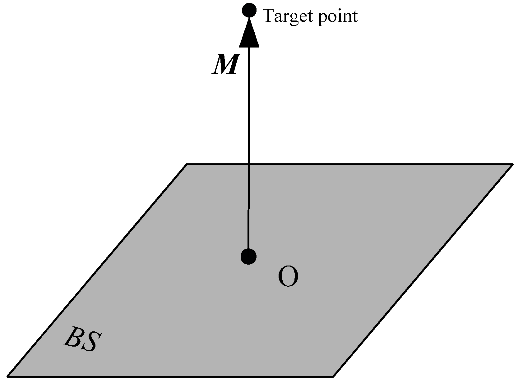
1.1. Model of Magnetic Tensor Localization

Model of STLM

The magnetic field $B$ at any point in the magnetic dipole space can be expressed as the following [14,15]:

$$B=\frac{{\mu }_0}{4\pi r^3}[3(M\cdot r_0)r_0-M]$$

(1)

In Equation (1), ${\mu }_0$ is the magnetic permeability of vacuum, ${\mu }_0\approx 4\pi \times 10^{-7} \mathrm{H}/\mathrm{m}$ is in air, M is the magnetic moment vector of the magnetic target, $r=\left|\mathit{r}\right|$ is the value of the distance vector modulus $r$ between the magnetic target and the detection point, and $r_0=\raisebox{1ex}{$r$}\!\left/ \!\raisebox{-1ex}{$r$}\right.$ is the unit vector of $r$.

The space change rate of the three mutually orthogonal directions of the magnetic vector field is the magnetic tensor [16], which is the vector magnetic gradient, including nine elements in total. The magnetic tensor $G$ of magnetic vector field $B$ can be expressed as the following:

$$G=\left[\begin{array}{ccc}\frac{\partial B_x}{\partial x}& \frac{\partial B_x}{\partial y}& \frac{\partial B_x}{\partial z}\\ \frac{\partial B_y}{\partial x}& \frac{\partial B_y}{\partial y}& \frac{\partial B_y}{\partial z}\\ \frac{\partial B_z}{\partial x}& \frac{\partial B_z}{\partial y}& \frac{\partial B_z}{\partial z}\end{array}\right]=\left[\begin{array}{ccc}{G}_{xx}& G_{xy}& G_{xz}\\ G_{yx}& G_{yy}& G_{yz}\\ G_{zx}& G_{zy}& G_{zz}\end{array}\right]$$

(2)

In Equation (2), $B_x$, $B_y$, and $B_z$ are the three components of the magnetic field at any point $\left(x,y,z\right)$ in space, and $G_{ij}\left(i,j=x,y,z\right)$ are the components of the magnetic tensor.

It can be seen from Maxwell’s equations that, in the passive environmental static magnetic field, the divergence and curl of the magnetic field are both zero. Only five elements, $G_{xx}$, $G_{xy}$, $G_{xz}$, $G_{yy}$, and $G_{yz}$, can be calculated to obtain the magnetic tensor of the magnetic field, namely:

$$G=\left[\begin{array}{ccc}{G}_{xx}& G_{xy}& G_{xz}\\ G_{yx}& G_{yy}& G_{yz}\\ G_{zx}& G_{zy}& G_{zz}\end{array}\right]=\left[\begin{array}{ccc}{G}_{xx}& G_{xy}& G_{xz}\\ G_{xy}& G_{yy}& G_{yz}\\ G_{xz}& G_{yz}& -G_{xx}-G_{yy}\end{array}\right]$$

(3)

The positioning formula of STLM [17]:

$$r=-3G^{-1}B$$

(4)

According to Equation (4), the location of the magnetic target can be calculated when the magnetic tensor and magnetic field vector value of a point is known. The algorithm of STLM is simple in calculation and has high efficiency during positioning. However, it is greatly affected by the geomagnetic field, which greatly limits the application of the method [18,19,20].

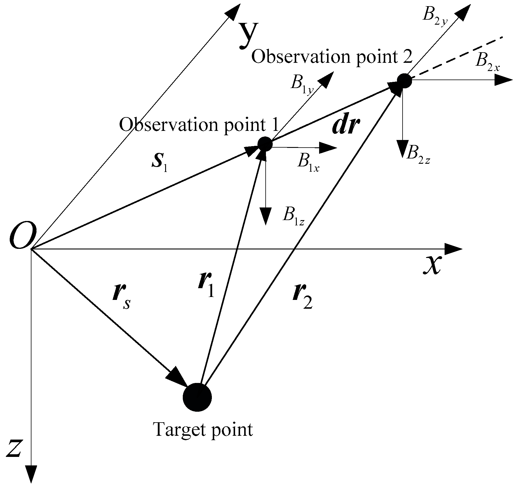
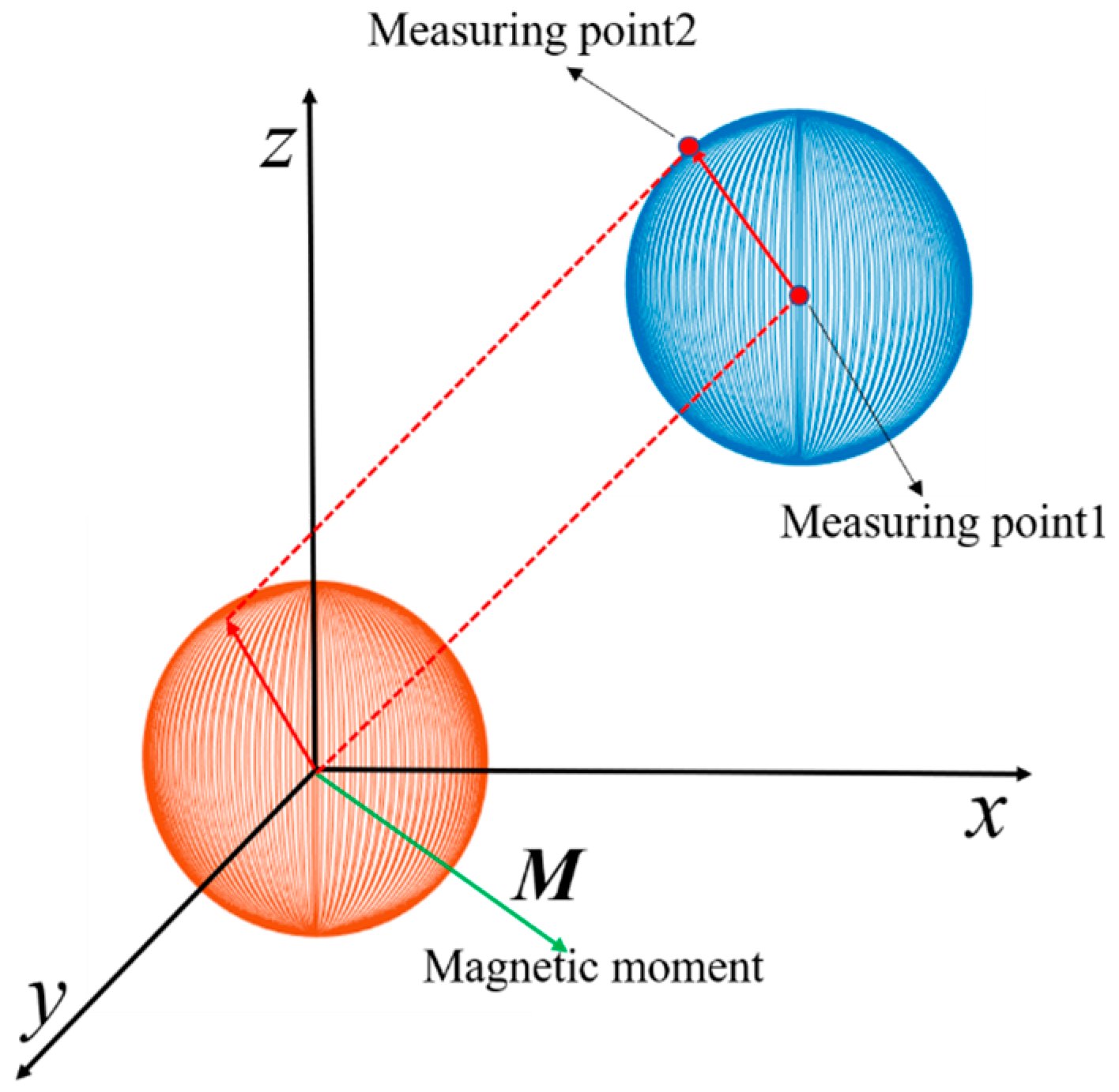
1.2. Model of TTLM

The model of TTLM is shown in Figure 1. A random point in space is set as the origin, the position of the target point is set as $r_s$, the relative position of the observation point 1 and the target point is $r_1$, the relative position of the observation point 2 and the target point is $r_2$, and the relative position vector relationship between the two observation points is as follows [21]:

$$r_2=r_1+dr$$

(5)

The formula of TTLM is

$$r_1=-{(G_2-G_1)}^{-1}(3G_1+G_2)dr$$

(6)

$G_1$ and $G_2$ represent the magnetic tensors of observation point 1 and observation point 2, respectively. Combining the positioning model of Equation (6) and Figure 1, we can obtain the positioning formula of the target point as follows:

$$r_s=S_1-r_1$$

(7)

According to Equations (6) and (7), we can use the two-point magnetic tensor and the relative position of the two points to locate the target point. During this period, we do not need to measure the value of the geomagnetic field, which reduces the positioning error of the geomagnetic field noise. In addition, we use a linear method to complete the solution. The solution process is simple, and we can directly obtain an analytical solution.

2. Blind Spots Analysis of Location

On the one hand, the basis of realizing the STIM, according to Equation (4), is that the magnetic tensor value $G$ at the detection point is reversible; on the other hand, the basis of realizing the TTLM, according to Equations (6) and (7), is that the magnetic tensor difference $(G_2-G_1)$ between two detection points is reversible. When the magnetic tensor matrix or magnetic tensor difference matrix is irreversible, the positioning formula is not valid. The positioning method will be invalid, and location cannot be achieved. Such points that cannot be located by using the magnetic tensor positioning method are called magnetic tensor positioning blind spots.

2.1. Blind Spots Analysis of STLM

Taking the coordinates of each point into Equation (2), the component expression of the magnetic tensor $G_1$ of a single point can be obtained as the following:

$$\left[\begin{array}{c}{G}_{1xx}\\ G_{1xy}\\ G_{1xz}\\ G_{1yy}\\ G_{1yz}\end{array}\right]=\frac{{\mu }_0}{4\pi r_1^7}\left[\begin{array}{ccc}9x_1{r}_1^2-15x_1^3& 3y_1{r}_1^2-15x_1^2{y}_1& 3z_1{r}_1^2-15x_1^2{z}_1\\ 3y_1{r}_1^2-15x_1^2{y}_1& 3x_1{r}_1^2-15x_1{y}_1^2& -15x_1{y}_1{z}_1\\ 3z_1{r}_1^2-15x_1^2{z}_1& -15x_1{y}_1{z}_1& 3x_1{r}_1^2-15x_1{z}_1^2\\ 3x_1{r}_1^2-15x_1{y}_1^2& 9y_1{r}_1^2-15y_1^3& 3z_1{r}_1^2-15y_1^2{z}_1\\ -15x_1{y}_1{z}_1& 3z_1{r}_1^2-15y_1^2{z}_1& 3y_1{r}_1^2-15y_1{z}_1^2\end{array}\right]\left[\begin{array}{c}{m}_x\hfill \\ m_y\hfill \\ m_z\hfill \end{array}\right]$$

(8)

$r_1=(x_1,y_1,z_1)$ is the position of the target and $m=(m_x,m_y,m_z)$ is the moment of the target. According to Equations (3) and (8), the eigenvalue of $G_1$ can be calculated as follows:

$$\left\{\begin{array}{cc}\hfill {\lambda }_{11}=& \frac{-3}{2{\left(x_1^2+y_1^2+z_1^2\right)}^{5/2}}\left(\left(x_1{m}_x+y_1{m}_y+z_1{m}_z\right)+\left(9x_1^2{m}_x^2+4y_1^2{m}_x^2+4z_1^2{m}_x^2\right.\right.\hfill \\ \hfill & +10x_1{y}_1{m}_x{m}_y+4x_1^2{m}_y^2+9y_1^2{m}_y^2+4z_1^2{m}_y^2+10x_1{z}_1{m}_x{m}_z+10y_1{z}_1{m}_y{m}_z+\hfill \\ \hfill & \left.{\left.4x_1^2{m}_z^2+4y_1^2{m}_z^2+9z_1^2{m}_z^2\right)}^{1/2}\right)\hfill \\ \hfill {\lambda }_{12}=& \frac{3\left(x_1{m}_x+y_1{m}_y+z_1{m}_z\right)}{{\left(x_1^2+y_1^2+z_1^2\right)}^{5/2}}\hfill \\ \hfill {\lambda }_{13}=& \frac{-3}{2{\left(x_1^2+y_1^2+z_1^2\right)}^{5/2}}\left(\left(x_1{m}_x+y_1{m}_y+z_1{m}_z\right)-\left(9x_1^2{m}_x^2+4y_1^2{m}_x^2+4z_1^2{m}_x^2\right.\right.\hfill \\ \hfill & +10x_1{y}_1{m}_x{m}_y+4x_1^2{m}_y^2+9y_1^2{m}_y^2+4z_1^2{m}_y^2+10x_1{z}_1{m}_x{m}_z+10y_1{z}_1{m}_y{m}_z+\hfill \\ \hfill & \left.{\left.4x_1^2{m}_z^2+4y_1^2{m}_z^2+9z_1^2{m}_z^2\right)}^{1/2}\right)\hfill \end{array}\right.$$

(9)

${\lambda }_{11}$, ${\lambda }_{12}$, and ${\lambda }_{13}$ represent the three eigenvalues of the outgoing magnetic tensor matrix at a single measuring point. According to the expression of eigenvalues, when the direction of any measuring point is perpendicular to the direction of the target magnetic moment, there is $(x{m}_x+y{m}_y+z{m}_z)=0$, and the value ${\lambda }_{12}$ is zero. This shows that there must be an irreversible magnetic tensor matrix $G_1$, which produces a singular matrix. At this time, Equation (4) becomes an ill-conditioned equation, and the single-point magnetic tensor positioning method is invalid, so the target cannot be located, and blind spots are generated.

Because the magnetic target moment is a vector with a fixed size, the points perpendicular to it can form a plane. The location blind surface is formed by the location blind spots. A location blind surface is a plane passing through the coordinate origin and perpendicular to the target magnetic moment, as shown in Figure 2.

In Figure 2, $O$ is the position of the coordinate origin, $M$ is the magnetic target moment, and $BS$ (blind surface) is the blind surface that cannot be located using the STLM. When the measurement system moves to the blind surface, the position of the target point obtained by using STLM will greatly differ from the actual target point position, and the positioning result will be unreliable.

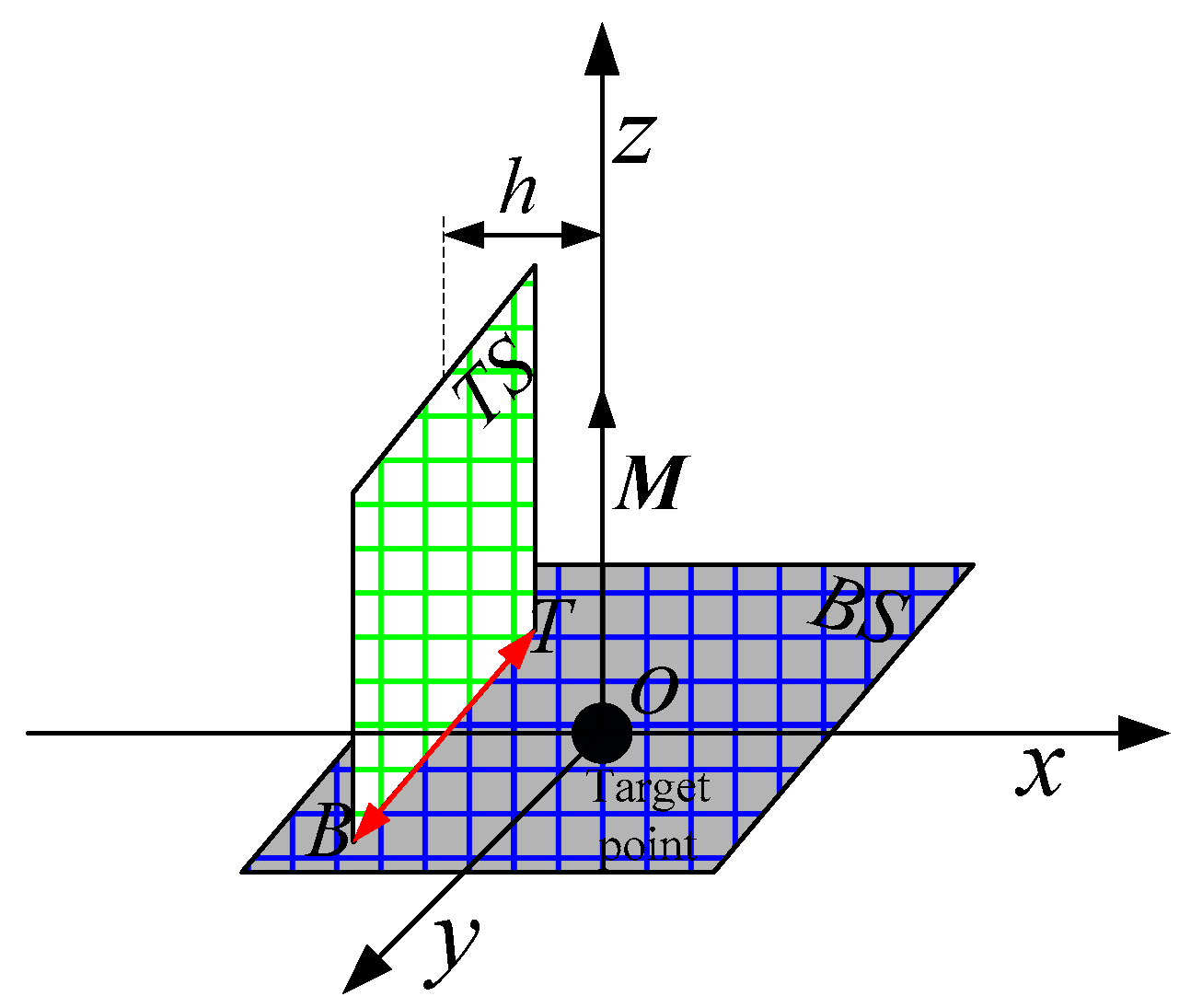
2.2. Blind Spots Analysis of TTLM

For the TTLM, the component expression of $G_2$ is the following:

$$\left[\begin{array}{c}{G}_{2xx}\\ G_{2xy}\\ G_{2xz}\\ G_{2yy}\\ G_{2yz}\end{array}\right]=\frac{{\mu }_0}{4\pi r_2^7}\left[\begin{array}{ccc}9x_2{r}_2^2-15x_2^3& 3y_2{r}_2^2-15x_2^2{y}_2& 3z_2{r}_2^2-15x_2{}^2{z}_2\\ 3y_2{r}_2^2-15x_2^2{y}_2& 3x_2{r}_2^2-15x_2{y}_2^2& -15x_2{y}_2{z}_2\\ 3z_2{r}_2^2-15x_2^2{z}_2& -15x_2{y}_2{z}_2& 3x_2{r}_2^2-15x_2{z}_2{}^2\\ 3x_2{r}_2^2-15x_2{y}_2^2& 9y_2{r}_2^2-15y_2{}^3& 3z_2{r}_2^2-15y_2^2{z}_2\\ -15x_2{y}_2{z}_2& 3z_2{r}_2^2-15y_2{}^2{z}_2& 3y_2{r}_2^2-15y_2{z}_2^2\end{array}\right]\left[\begin{array}{c}{m}_x\hfill \\ m_y\hfill \\ m_z\hfill \end{array}\right]$$

(10)

The subscript number in Equations (8) and (10) represents the position of the detection point. The relationship between the coordinates is as follows:

$$\left\{\begin{array}{l}{r}_1=\sqrt{x_1{}^2+y_1{}^2+z_1{}^2}\\ x_2=x_1+\Delta x\\ y_2=y_1+\Delta y\\ z_2=z_1+\Delta z\\ r_2=\sqrt{x_2{}^2+y_2{}^2+z_2{}^2}\end{array}\right.$$

(11)

$\Delta x,\Delta y,\Delta z$ are the distances of one point and another. It can be obtained using Equations (8) and (10) that the difference between the two magnetic tensor components is the following:

$$\begin{array}{c}\Delta G_c=G_2-G_1=\left[\begin{array}{ccc}{G}_{2xx}-G_{1xx}& G_{2xy}-G_{1xy}& G_{2xz}-G_{1xz}\\ G_{2xy}-G_{1xy}& G_{2yy}-G_{1yy}& G_{2yz}-G_{1yz}\\ G_{2xz}-G_{1xz}& G_{2yz}-G_{1yz}& -G_{2yy}+G_{1yy}-G_{2xx}+G_{1xx}\end{array}\right]\\ =\left[\begin{array}{ccc}\Delta G_{xx}& \Delta G_{xy}& \Delta G_{xz}\\ \Delta G_{xy}& \Delta G_{yy}& \Delta G_{yz}\\ \Delta G_{xz}& \Delta G_{yz}& -\Delta G_{xx}-\Delta G_{yy}\end{array}\right]\end{array}$$

(12)

By analyzing Equations (8), (10) and (12), it is found that it is very difficult to analyze the blind spot of TTLM theoretically, and it is difficult to obtain a fixed parameter relationship using the blind spot analysis process of STLM. Therefore, a spherical analysis method is proposed to analyze the blind spot of STLM.

Because the blind spot position of the TTLM cannot be determined, the blind spot existence condition of the STLM is referred to during the analysis. The condition is that the magnetic moment is perpendicular to the vector formed by the measuring points. At the same time, in order to not be limited to the condition of perpendicularity and take full account of other included angles, we used a spherical model around the first point for ensuring the existence of any included angle, as shown in Figure 3. We took any point on the spherical equation as the second measuring point, then any vector composed of these two points must form any angles with the magnetic moment so that the positioning analysis of any angles can be completed. Then, we used this principle to analyze the blind spot of TTLM, which is called the spherical analysis method.

3. Blind Spots Simulation of Location

3.1. Simulation of STLM

In order to visually see the existence of blind spots and blind surfaces, the magnetic dipole model and STLM model are used for simulation analysis. In the simulation, assuming that the magnetic target is a magnetic dipole and is at the origin of the coordinate system, use Equation (4) to calculate the position coordinates of the measurement system relative to the magnetic target. According to the principle of two-point relativity, the position coordinates of the magnetic target relative to the measurement system can be determined.

As shown in Figure 4, the coordinate system is established with the magnetic dipole as the coordinate origin. The magnetic moment of the magnetic target is $M$, the detection plane $TS$ is parallel to $M$, the distance is $h$, and $BS$ is the theoretical positioning blind surface. The red double arrow line $BT$ is the intersection line between the positioning blind surface and the detection plane. The detection plane $TS$ is discretized into multiple detection points, and the magnetic tensor at each detection point is obtained. The magnetic target position is calculated using the STLM. When the detection point is on $BT$, the positioning error will increase sharply, and the positioning cannot be realized.

During the simulation, some detection points of the measurement system in the process of movement are on the blind surface. The relative errors in three directions are used to evaluate the positioning effect of this simulation. $(x,y,z)$ is the real position coordinates of the magnetic target, and $(x_m,y_m,z_m)$ is the calculated position coordinates. The error formulas are as follows:

$$\left\{\begin{array}{l}Errx=x-x_m\\ Erry=y-y_m\\ Errz=z-z_m\end{array}\right.$$

(13)

Set the target magnetic moments to $m_x=0$, $m_y=0$, $m_z=500$ A·m², and $h=40$ m, and the blind surface to $z=0$. Suppose that the measurement system is located in the detection plane to measure the magnetic tensor, and it moves up and down on the intersection line $BT$. At this time, the coordinates of $x$ are −40 m, the coordinates of axis $y$ are −20~20 m, and the coordinates of axis $z$ are −20~20 m. The data of axis $y$ and axis $z$ are scattered to form an array of measuring points so that the points in the array whose axis $z$ coordinate is zero appear in a circle. The positioning error obtained by simulation is shown in Figure 5.

In Figure 5, axis $y$ and axis $z$ of the horizontal plane represent the coordinates of the detection point, and the vertical axes $Errx$, $Erry$, and $Errz$ of ($a$), ($b$), and ($c$) are the positioning errors of axis $x$, $y$, and $z$, respectively. It can be seen from the figure that, in the detection area of $z\ne 0$, the location errors in three directions fluctuate around zero, and the fluctuation value is very small. However, the location error in the three directions of a point on the area of $z=0$ becomes a blank area, which cannot be located. It shows that when the magnetic measurement system passes through the point on the intersection line between the detection plane and the blind surface, the location error of STLM is large, and the positioning result is unreliable.

The simulation results show that blind spots do exist when using the STLM to determine the magnetic target position. Therefore, when using this positioning method to locate the magnetic target, the points on the blind surface should be reasonably avoided to prevent positioning failure.

3.2. Simulation of TTLM

Firstly, the spherical analysis method is used to verify the existence of blind spots in the STLM. Set the magnetic moment of the magnetic dipole as $M=(167,448,100) \mathrm{A}\cdot {\mathrm{m}}^2$. The magnetic target is located at the coordinate origin, and the measuring point is located on a sphere with a radius of 40 m. The spherical equation is as follows:

$$\left\{\begin{array}{c}x=40\sin \left({\psi }_s\right)\cos \left({\theta }_s\right)\\ y=40\sin \left({\psi }_s\right)\sin \left({\theta }_s\right)\\ z=40\sin \left({\theta }_s\right)\end{array}\right.$$

(14)

In Equation (14), ${\psi }_s$ and ${\theta }_s$ are the parameters that constitute the sphere, and the range of setting them is $0~\pi$ and $0~2\pi$, respectively. The simulation results are shown in Figure 6.

In Figure 6, the vertical axes of ($a$), ($b$), and ($c$) are the positioning relative error in the $x$, $y$, and $z$ directions, respectively, and the horizontal axis is the simulation times. It can be seen from the figure that although the relative error of the $y$-axis is kept at a low level during the positioning process by using the points on the sphere, the relative error of the $x$-axis positioning reaches $3\times {10}^4\%$, and the relative error of the $z$-axis positioning reaches $2.5\times {10}^{19}\%$. There are large errors in coordinate positioning, and there are blind spots, so it is impossible to complete the positioning.

The spherical analysis method shows that the STLM does have blind spots, which is consistent with the simulation results in Section 2.1, indicating that the analysis method can effectively analyze the blind spot characteristics of the positioning method. Therefore, the spherical analysis method is used to analyze the blind spots of the TTLM. Set the magnetic moment of the magnetic dipole as $M=(167,448,100) \mathrm{A}\cdot {\mathrm{m}}^2$; the magnetic target is located at (18, 26, and 30) m, the position of measuring point 1 is (1, 2, and 3) m, and the measuring point 2 is located on the spherical surface with a radius of 0.1 m centered on measuring point 1. The spherical equation is as follows:

$$\left\{\begin{array}{l}x=1+0.1\sin ({\psi }_s)\cos ({\theta }_s)\\ y=2+0.1\sin ({\psi }_s)\sin ({\theta }_s)\\ z=3+0.1\sin ({\theta }_s)\end{array}\right.$$

(15)

The parameter ranges of ${\psi }_s$ and ${\theta }_s$ are $0~\pi$ and $0~2\pi$, respectively. The simulation results are shown in Figure 7. The vertical axis of $(a)$, $(b)$, and $(c)$ in the figure are the relative positioning errors in the $x$, $y$, and $z$ directions, respectively, and the horizontal axis is the simulation times.

It can be seen from Figure 7 that the relative positioning errors in the x-axis, y-axis, and z-axis directions are kept at a low level. The maximum relative positioning error exists in the x-axis direction but is only 5%, which is far less than the relative error caused by the measurement error. The probability that this point is a blind spot is very small; therefore, it is reasonable to think that the magnetic target location can still be accurately determined by using the TTLM if there is a blind spot in a fixed area by STLM.

Of course, in the process of using the magnetic tensor measurement system to actually detect the target (because the carrier can hardly strictly keep moving in a fixed plane perpendicular to the magnetic moment even if a single point exists in the blind surface to cause a positioning failure problem), several adjacent points can be used to calculate the magnetic target position to achieve the positioning purpose.

4. Conclusions

In this paper, by studying the STLM and the TTLM, the blind spots of the two localization methods are analyzed. The eigenvalue analysis method is used to analyze the blind spot of STLM. The results show that when the direction of any measuring point is perpendicular to the direction of the target magnetic moment, the magnetic tensor matrix is irreversible, the STLM is invalid, and blind spots appear. At the same time, the spherical analysis method is proposed to analyze the blind spot of the TTLM. The simulation results show that the STLM has an obvious blind spot while TTLM still has good positioning performance in the blind spot.

References

- Sheinker, A.; Ginzburg, B.; Salomonski, N.; Frumkis, L.; Kaplan, B.Z.; Moldwin, M.B. Method for indoor navigation based on magnetic beacons using smartphones and tablets. Measurement 2016, 81, 197–209. [Google Scholar] [CrossRef]
- Yin, G.; Zhang, Y.; Fan, H. Localization and Classification of Multiple Dipole-Like Magnetic Sources Using Magnetic Gradient Tensor Data. J. Appl. Geophys. 2016, 128, 131–139. [Google Scholar]
- Yu, H.; Li, H.; Feng, S. Underwater Continuous Localization Based on Magnetic Dipole Target Using Magnetic Gradient Tensor and Draft Depth. IEEE Geosci. Remote Sens. Lett. 2014, 11, 178–180. [Google Scholar]
- Clark, D.A. New Methods for Interpretation of Magnetic vector and Gradient Tensor Data I: Eigenvector Analysis and the Normalized Source Strength. Explor. Geo-Phys. 2012, 44, 267–282. [Google Scholar] [CrossRef]
- Liu, H.; Wang, X.; Wang, H.; Bin, J.; Dong, H.; Ge, J.; Liu, Z.; Yuan, Z.; Zhu, J.; Luan, X. Magneto-Inductive Magnetic Gradient Tensor System for Detection of Ferromagnetic Objects. IEEE Magn. Lett. 2020, 11, 8101205. [Google Scholar] [CrossRef]
- Li, J.; Zhang, Y.; Fan, H.; Li, Z. Preprocessed Method and Application of Magnetic Gradient Tensor Data. IEEE Access 2019, 7, 173738–173752. [Google Scholar] [CrossRef]
- Jeffrey, G.T.; William, D.E. Initial design and testing of a full tensor airborne SQUID magnetometer for detection of unexploded ordnance. Seg Tech. Program Expand. Abstr. 2004, 23, 798–804. [Google Scholar]
- Smith, D.V.; Bracken, R.E. Field experiments with the tensor magnetic gradiometer system for UXO surveys A case history. Seg Tech. Program Expand. Abstr. 2004, 23, 806–809. [Google Scholar]
- Brown, P.J. A case study of magnetic gradient tensor invariants applied to the UXO problem. Seg Tech. Program Expand. Abstr. 2004, 23, 794–797. [Google Scholar]
- Chwala, A.; Schmelz, M.; Zakosarenko, V. Underwater operation of a full tensor SQUID gradiometer system. Supercond. Sci. Technol. 2018, 32, 024003. [Google Scholar] [CrossRef]
- McGary, J. Real-Time Tumor Tracking for Four-Dimensional Computed Tomography Using SQUID Magnetometers. IEEE Trans. Magn. 2009, 45, 3351–3361. [Google Scholar] [CrossRef]
- Stolz, R.; Zakosarenko, V.; Schulz, M.; Chwala, A.; Fritzsch, L.; Meyer, H.G.; Köstlin, E.O. Magnetic full-tensor SQUID gradiometer system for geophysical applications. Lead. Edge 2006, 25, 178–180. [Google Scholar] [CrossRef]
- Ge, J.; Wang, S.; Dong, H.; Liu, H.; Zhou, D.; Wu, S.; Luo, W.; Zhu, J.; Yuan, Z.; Zhang, H. Real-Time Detection of Moving Magnetic Target Using Distributed Scalar Sensor Based on Hybrid Algorithm of Particle Swarm Optimization and Gauss-Newton Method. IEEE Sens. J. 2020, 20, 10717–10723. [Google Scholar] [CrossRef]
- Nara, T.; Suzuki, S.; Ando, S. A Closed-Form Formula for Magnetic Dipole Localization by Measurement of Its Magnetic Field and Spatial Gradients. IEEE Trans. Magn. 2006, 42, 3291–3293. [Google Scholar] [CrossRef]
- Oruc, B. Location and depth estimation of point-dipole and line of dipoles using analytic signals of the magnetic gradient tensor and magnitude of vector components. J. Appl. Geophys. 2010, 70, 27–37. [Google Scholar] [CrossRef]
- Schmidt, P.W.; Clark, D.A. The magnetic gradient tensor:its properties and uses in source characterization. Lead. Edge 2006, 25, 75–78. [Google Scholar] [CrossRef]
- Wynn, W.M.; Frahm, C.P.; Clark, R.H. Advanced superconducting gradiometer magnetometer arrays and a novel signal processing technique. IEEE Trans. Magn. 1975, 11, 701–707. [Google Scholar] [CrossRef]
- Yan, Y.; Ma, Y.; Liu, J. Analysis and Correction of the Magnetometer Position Error in a Cross-Shaped Magnetic Tensor Gradiometer. Sensors 2020, 20, 1290. [Google Scholar] [CrossRef]
- Li, J.; Zhang, Y.; Fan, H.; Li, Z.; Liu, M. Estimating the location of magnetic sources using magnetic gradient tensor data. Explor. Geophys. 2019, 50, 600–612. [Google Scholar] [CrossRef]
- Liu, J.; Li, X.; Zeng, X. A Real-Time Magnetic Dipole Localization Method Based on Cube Magnetometer Array. IEEE Trans. Magn. 2019, 55, 4003609. [Google Scholar] [CrossRef]
- Xu, L.; Gu, H.; Fang, L.; Lin, P.; Lin, C. Magnetic Target Linear Location Method Using Two-Point Gradient Full Tensor. IEEE Trans. Instrum. Meas. 2021, 70, 6007808. [Google Scholar] [CrossRef]
Disclaimer/Publisher’s Note: The statements, opinions and data contained in all publications are solely those of the individual author(s) and contributor(s) and not of MDPI and/or the editor(s). MDPI and/or the editor(s) disclaim responsibility for any injury to people or property resulting from any ideas, methods, instructions or products referred to in the content. |
© 2023 by the authors. Licensee MDPI, Basel, Switzerland. This article is an open access article distributed under the terms and conditions of the Creative Commons Attribution (CC BY) license (https://creativecommons.org/licenses/by/4.0/).
Share and Cite
Xu, L.; Huang, X.; Dai, Z.; Yuan, F.; Wang, X.; Fan, J. Blind Spots Analysis of Magnetic Tensor Localization Method. Remote Sens. 2023, 15, 2199. https://doi.org/10.3390/rs15082199
Xu L, Huang X, Dai Z, Yuan F, Wang X, Fan J. Blind Spots Analysis of Magnetic Tensor Localization Method. Remote Sensing. 2023; 15(8):2199. https://doi.org/10.3390/rs15082199
Chicago/Turabian StyleXu, Lei, Xianyuan Huang, Zhonghua Dai, Fuli Yuan, Xu Wang, and Jinyu Fan. 2023. "Blind Spots Analysis of Magnetic Tensor Localization Method" Remote Sensing 15, no. 8: 2199. https://doi.org/10.3390/rs15082199