
Frequency Extraction of Global Constant Frequency Electromagnetic Disturbances from Electric Field VLF Data on CSES
 , ,
, ,
Abstract
:
1. Introduction
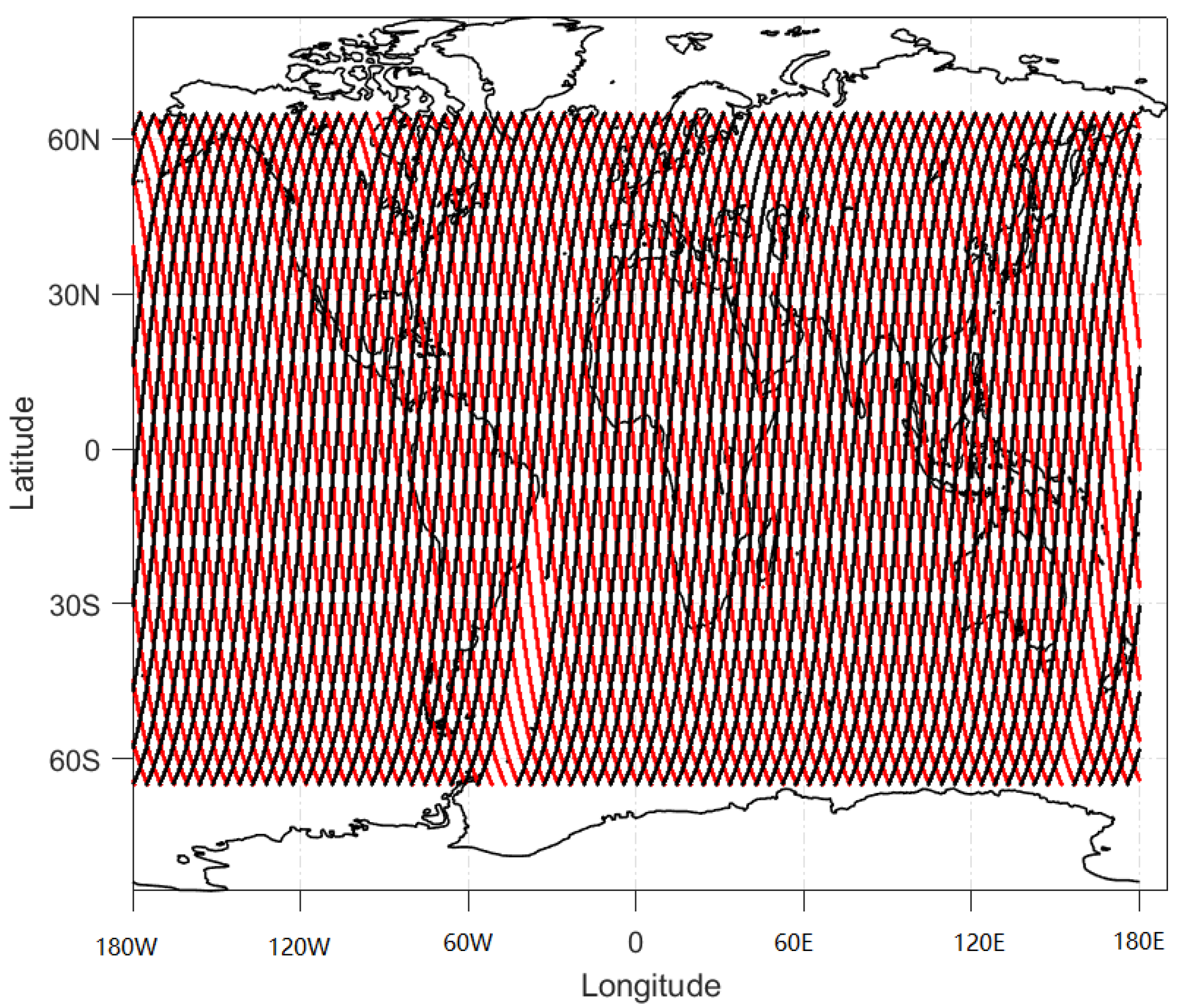
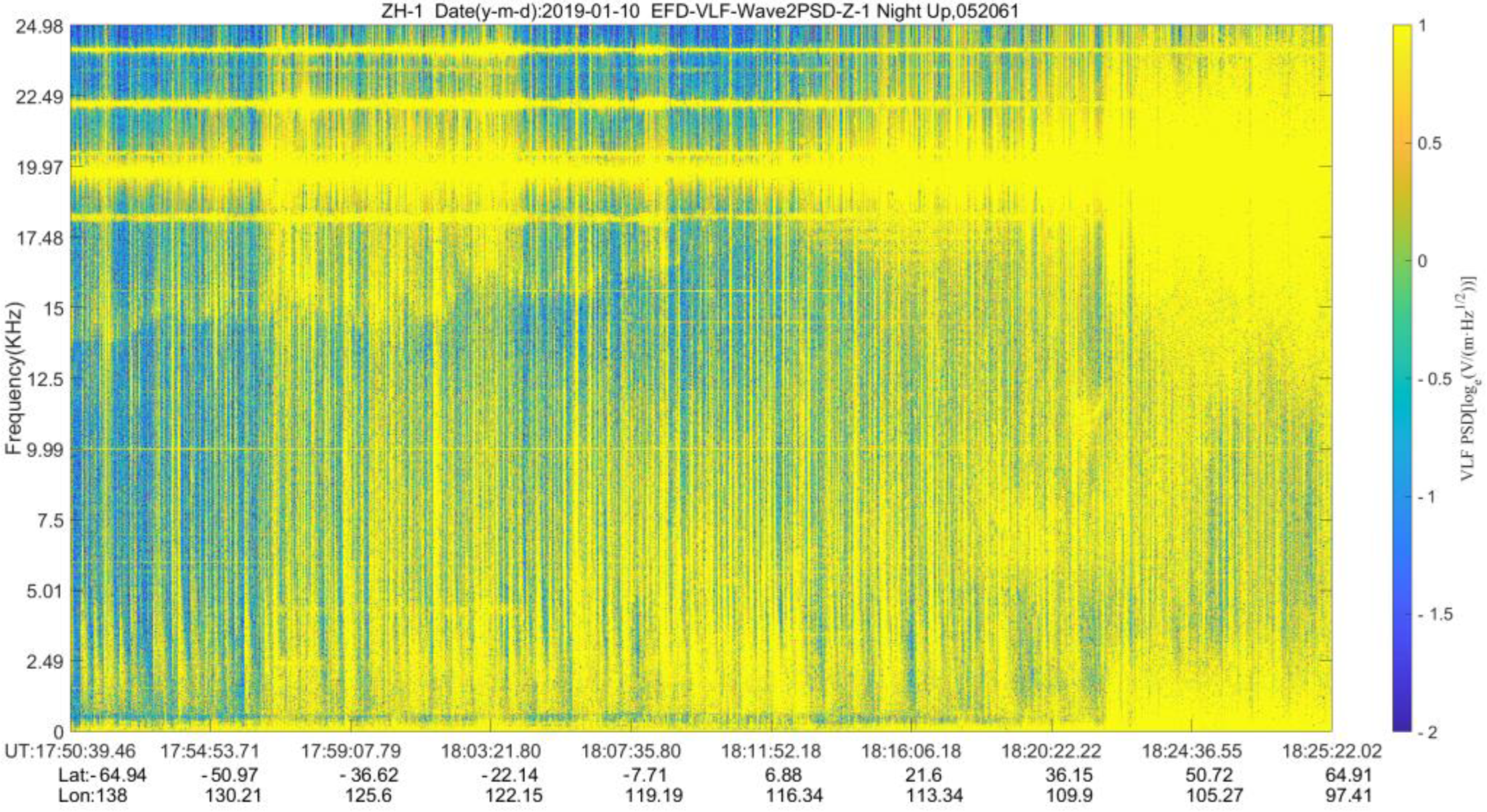
2. Data Collection
3. CFED Recognition Algorithm
3.1. Algorithm Identification Process
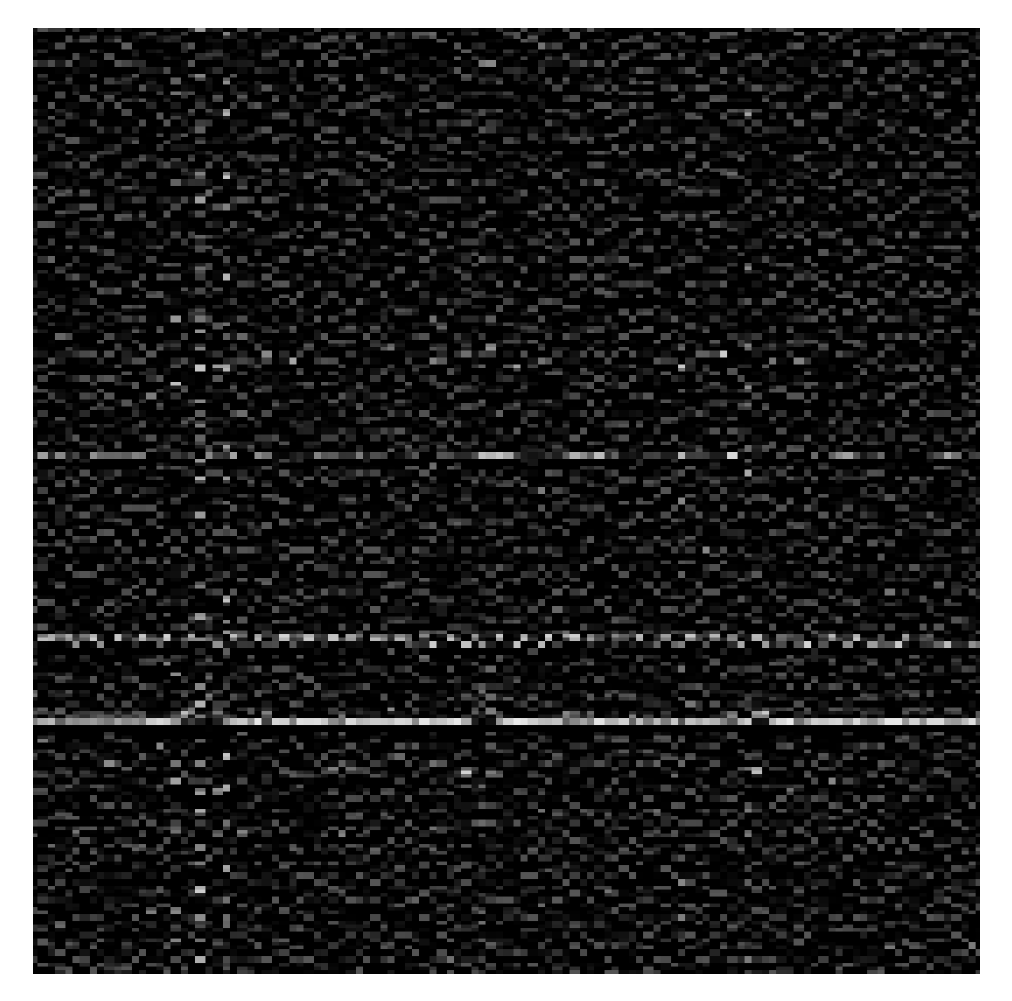
3.1.1. Gray Processing
3.1.2. Convolution Operation
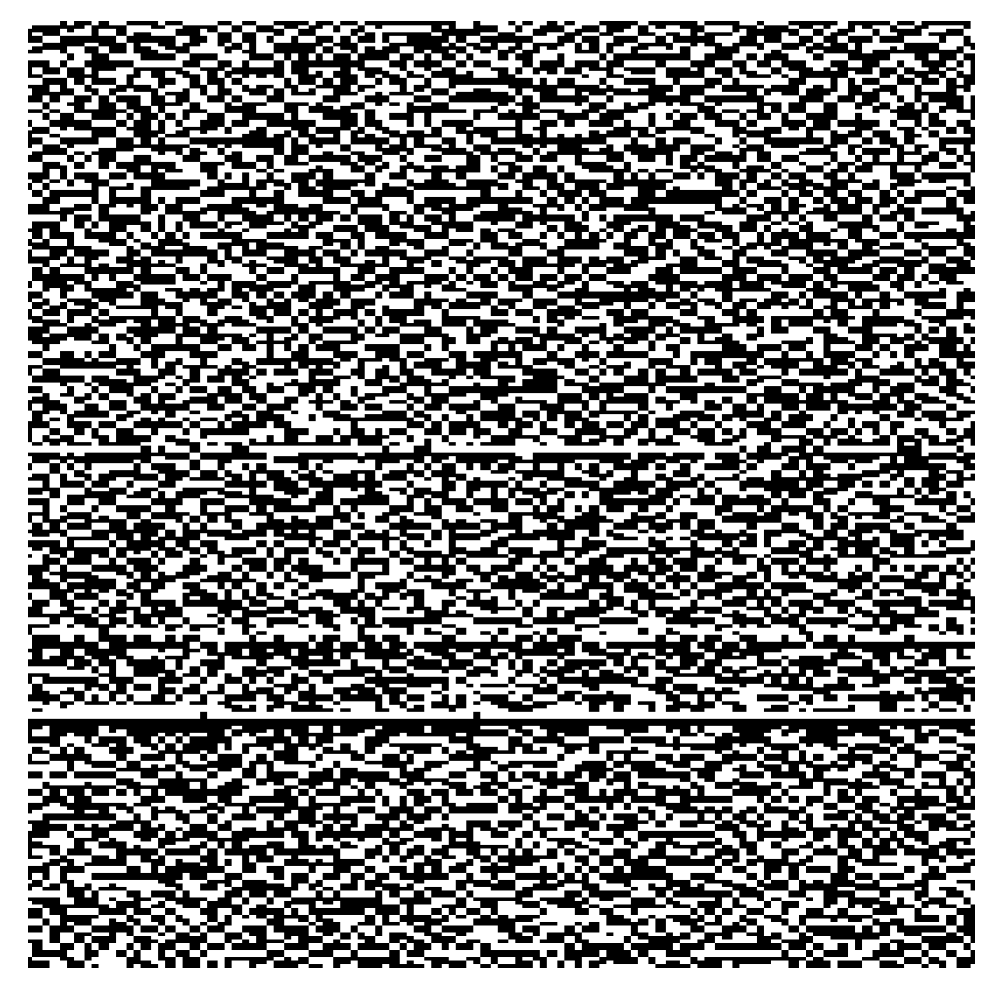
3.1.3. Binary Processing
3.1.4. K-Means Clustering
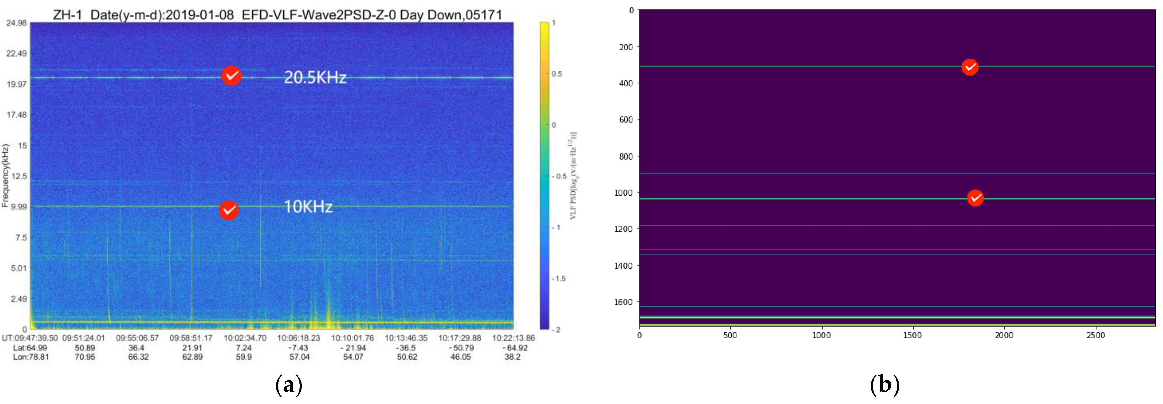
3.2. Extracting CFED Frequency from a Time–Frequency Spectrogram
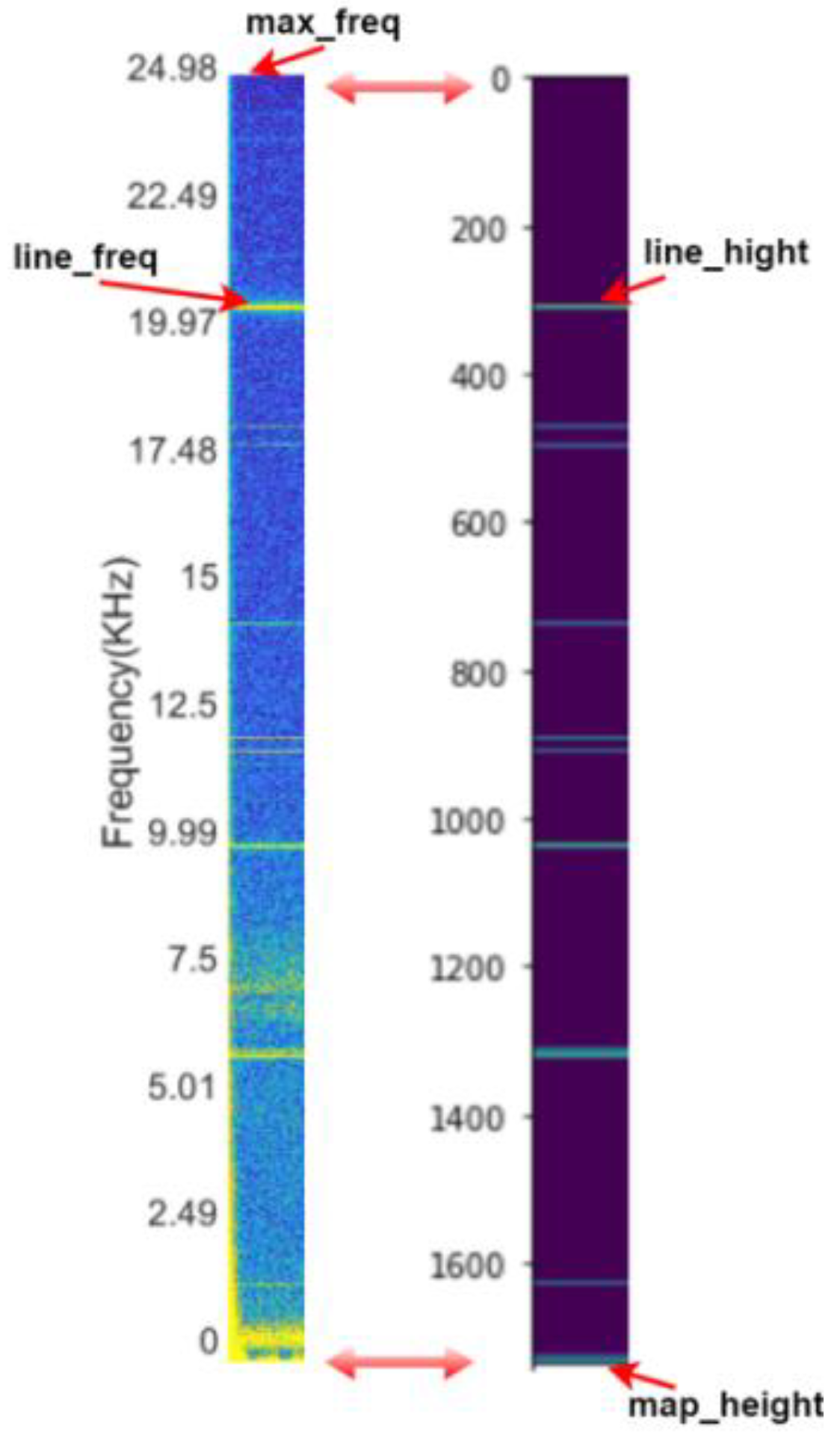
3.2.1. Extract the Frequency of a Pixel Row
3.2.2. Extract the Frequency Range of a Line Containing Continuous Multi-Pixel Rows
3.2.3. Extract all Horizontal Line Frequency Ranges for a Period (5 days)
3.2.4. Extract the Frequency Value by Power Spectrogram
4. Experimental Results and Analysis
4.1. Experimental Environment
4.2. Experimental Data
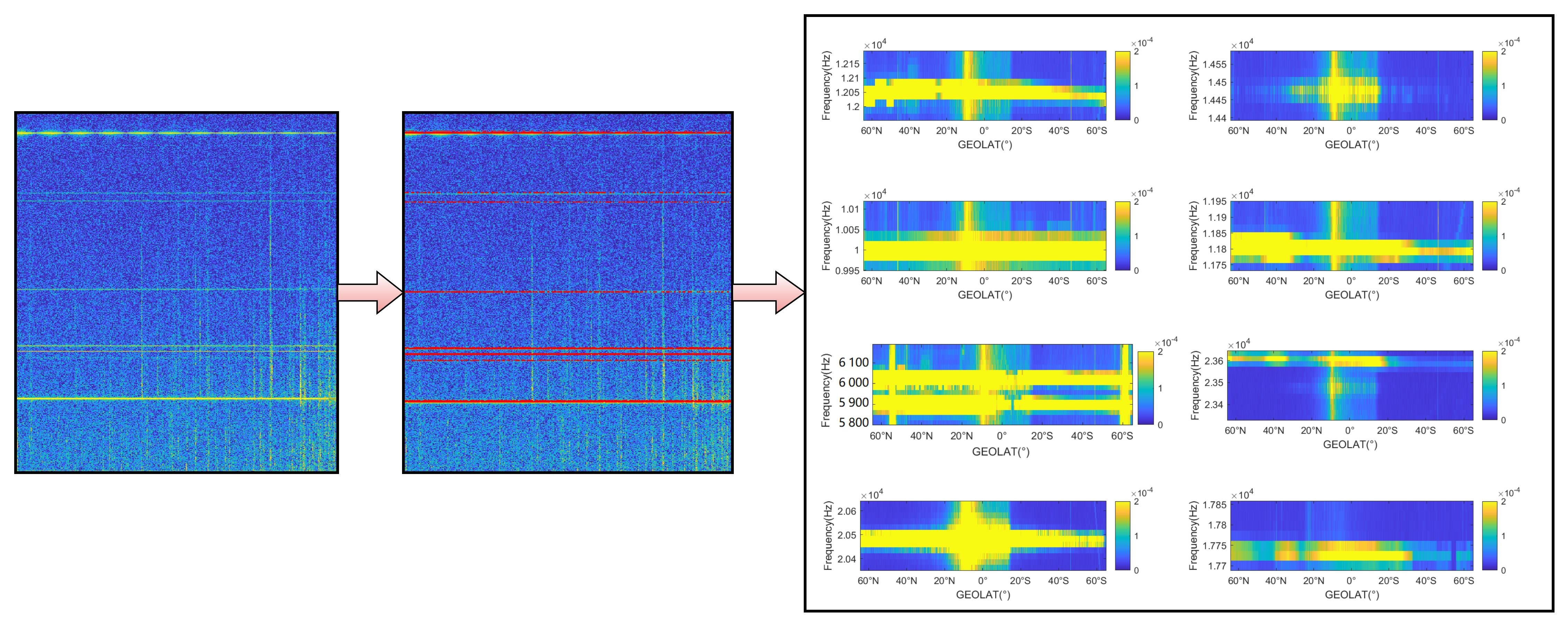
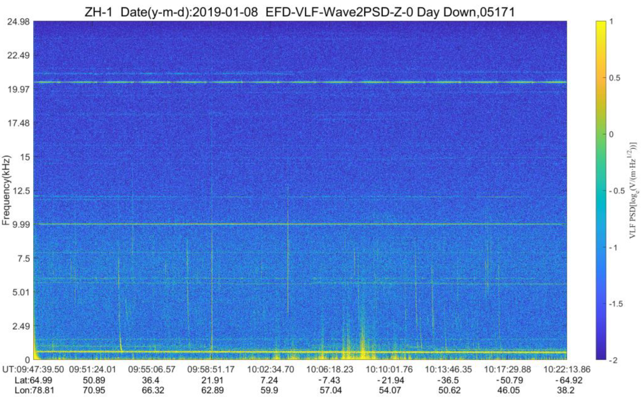
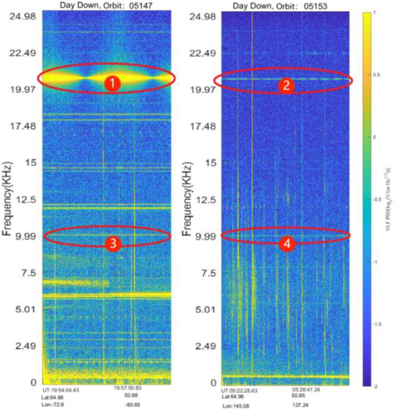
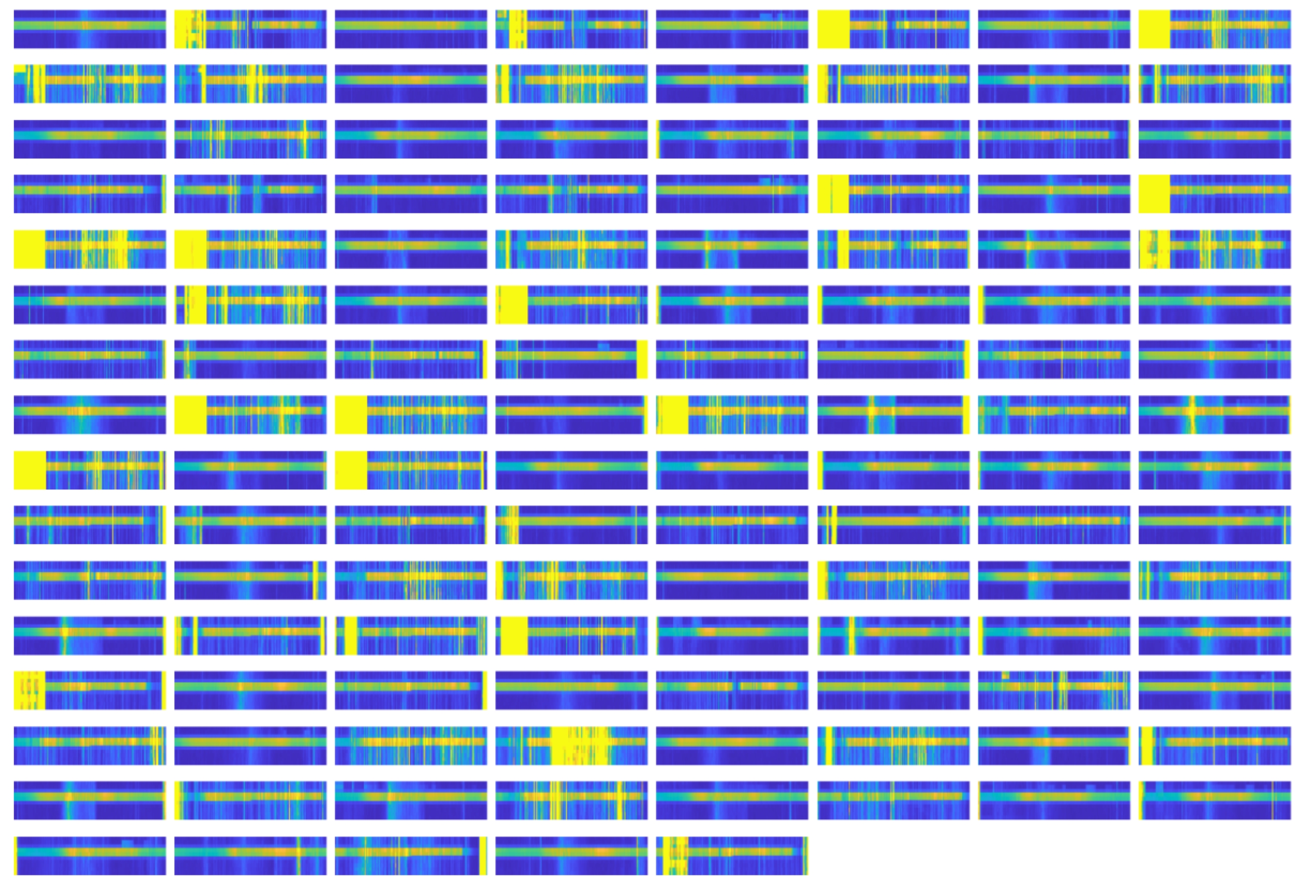
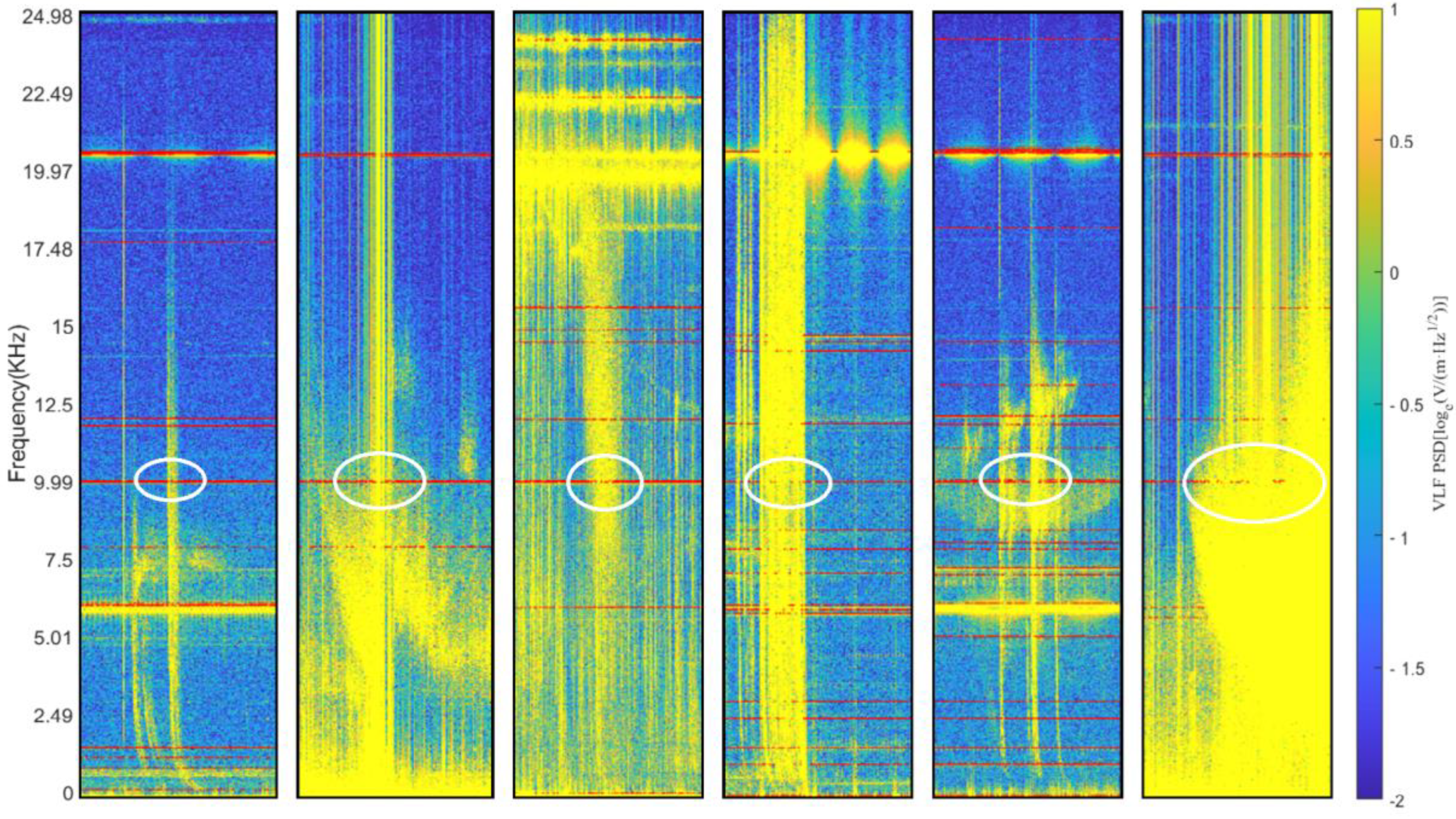
4.3. Recognize the Horizontal Lines
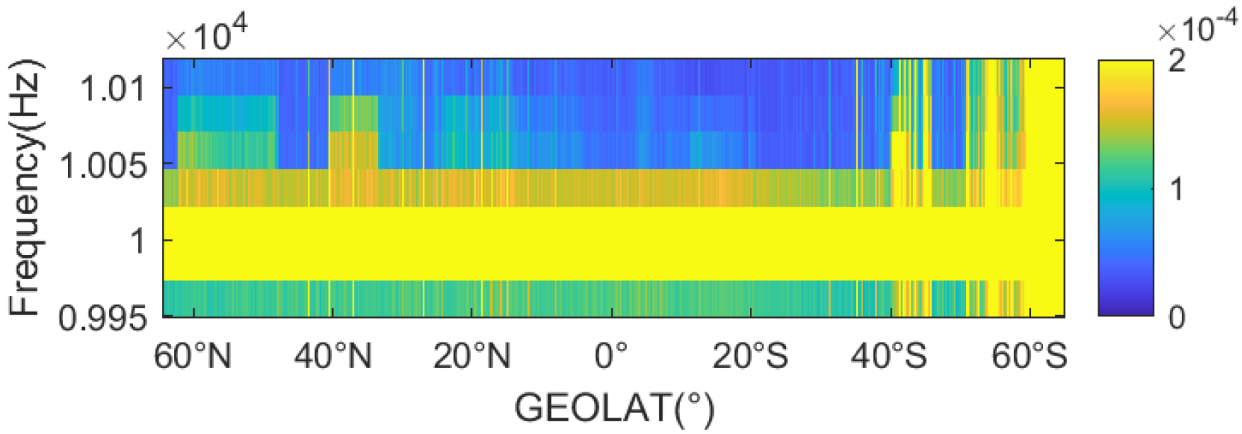
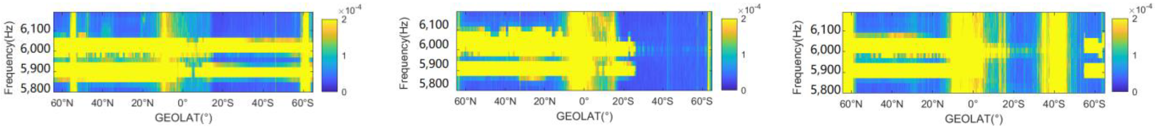
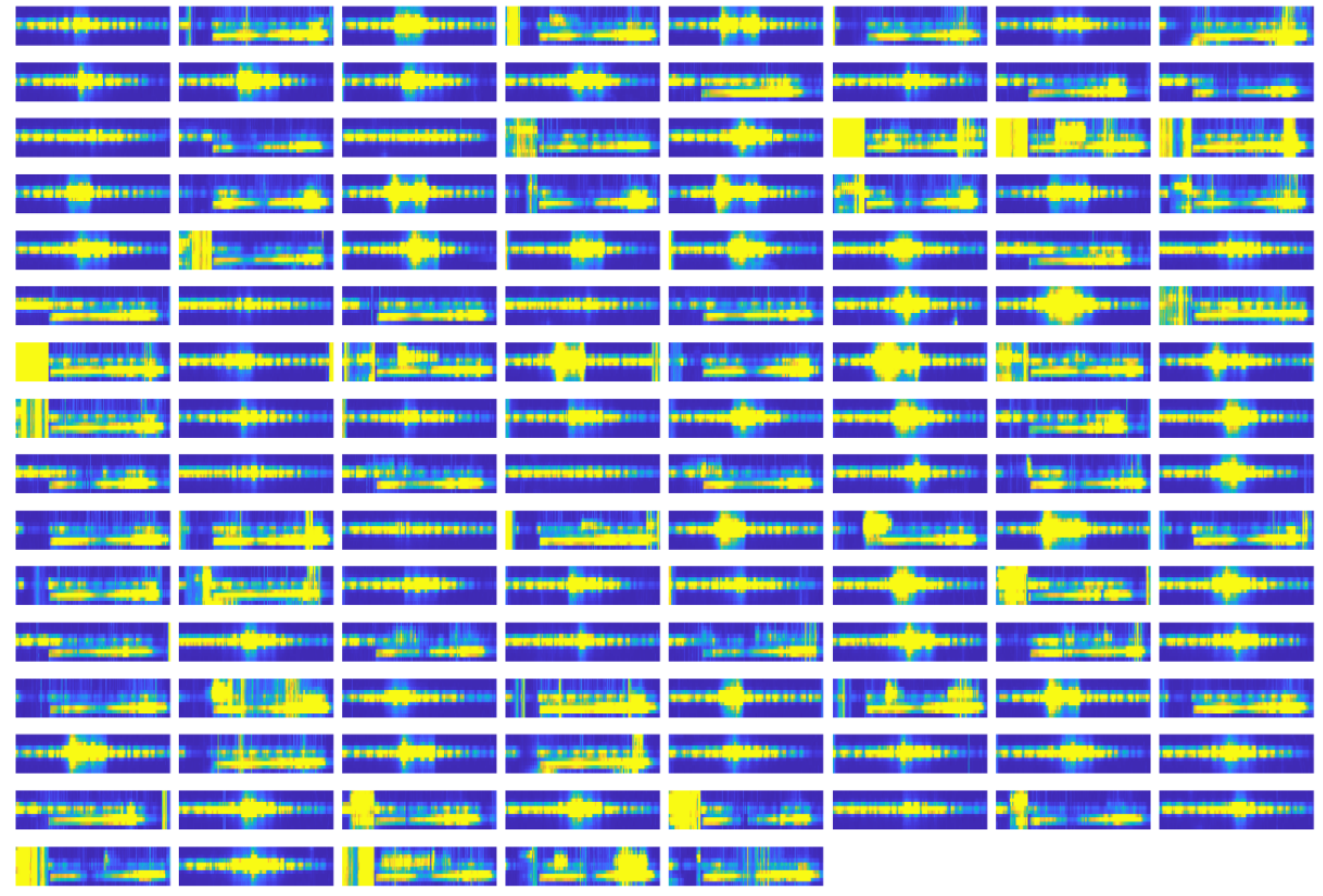
4.4. Extract the Frequency Range and Verify CFED Using a Power Spectrogram
4.5. Results Analysis
4.5.1. Reasons for the Low Occurrence of CFED Statistical Results
4.5.2. A Few Frequency Ranges Are Wide after Merging
4.5.3. CFEDs That Exist throughout the Period
5. Discussion
5.1. Frequency Value and CFED Localization Problem
5.2. Verification of CFED and the Extraction Frequency Method
5.3. Time–Frequency Spectrogram Orbit Data without Line Recognition
5.4. Other Space Electromagnetic Wave Disturbance Anomaly Detection
6. Conclusions
Author Contributions
Funding
Data Availability Statement
Acknowledgments
Conflicts of Interest
References
- Xiong, P.; Long, C.; Zhou, H.; Battiston, R.; Zhang, X.; Shen, X. Identification of Electromagnetic Pre-Earthquake Perturbations from the DEMETER Data by Machine Learning. Remote Sens. 2020, 12, 3643. [Google Scholar] [CrossRef]
- Ni, B.; Bortnik, J.; Thorne, R.M.; Ma, Q.; Chen, L. Resonant scattering and resultant pitch angle evolution of relativistic electrons by plasmaspheric hiss. J. Geophys. Res. Space Phys. 2013, 118, 7740–7751. [Google Scholar] [CrossRef]
- Ni, B.; Huang, H.; Zhang, W.; Gu, X.; Zhao, H.; Li, X.; Cao, X. Parametric sensitivity of the formation of reversed electron energy spectrum caused by plasmaspheric hiss. Geophys. Res. Lett. 2019, 46, 4134–4143. [Google Scholar] [CrossRef]
- Zhang, X.M.; Qian, J.D.; Shen, X.H.; Liu, J.; Wang, Y.L.; Huang, J.P.; Ouyang, X.Y. The seismic application progress in electromagnetic satellite and future development. Earthquake 2020, 40, 18–37. [Google Scholar]
- Otirakis, S.M.; Asano, T.; Hayakawa, M. Criticality analysis of the lower ionosphere perturbations prior to the 2016 Kumamoto (Japan) earthquakes as based on VLF electromagnetic wave propagation data observed at multiple stations. Entropy 2018, 20, 199. [Google Scholar] [CrossRef] [Green Version]
- Singh, V.; Hobara, Y. Simultaneous study of VLF/ULF anomalies associated with earthquakes in Japan. Open J. Earthq. Res. 2020, 9, 201–215. [Google Scholar] [CrossRef] [Green Version]
- Wang, S.; Gu, X.; Luo, F.; Peng, R.; Chen, H.; Li, G.; Yuan, D. Observations and analyses of the sunrise effect for NWC VLF transmitter signals. Chin. J. Geophys. 2020, 63, 4300–4311. [Google Scholar]
- Zhao, G.Z.; Lu, J.X. Monitoring and analysis of earthquake phenomena by artificial SLF Waves. Eng. Sci. 2003, 5, 27–32. [Google Scholar]
- Zhao, S.; Liao, L.; Zhang, X.; Shen, X. Full wave calculation of ground-based VLF radiation penetrating into the ionosphere. Chin. J. Radio Sci. 2016, 31, 825–833. [Google Scholar]
- Loudet, L. SID Monitoring Station[EB/OL]. 2013. Available online: https://sidstation.loudet.org/stations-list-en.xhtml (accessed on 18 June 2021).
- Cohen, M.B.; Inan, U.S.; Paschal, E.W. Sensitive broadband ELF/VLF radio reception with the AWESOME instrument. IEEE Trans. Geosci. Remote Sens. 2010, 48, 3–17. [Google Scholar] [CrossRef]
- Singh, R.; Veenadhari, B.; Cohen, M.B.; Pant, P.; Singh, A.K.; Maurya, A.K.; Vohat, P.; Inan, U.S. Initial results from AWESOME VLF receivers: Set up in low latitude Indian regions under IHY2007/UNBSSI program. Curr. Sci. 2010, 98, 398–405. [Google Scholar]
- Chen, Y.P.; Yang, G.B.; Ni, B.B.; Zhao, Z.Y.; Gu, X.D.; Zhou, C.; Wang, F. Development of ground-based ELF/VLF receiver system in Wuhan and its first results. Adv. Space Res. 2016, 57, 1871–1880. [Google Scholar] [CrossRef]
- Biagi, P.F.; Maggipinto, T.; Righetti, F.; Loiacono, D.; Schiavulli, L.; Ligonzo, T.; Ermini, A.; Moldovan, I.A.; Moldovan, A.S.; Buyuksarac, A.; et al. The European VLF/LF radio network to search for earthquake precursors: Setting up and natural/man-made disturbances. Nat. Hazards Earth Syst. Sci. 2011, 11, 333–341. [Google Scholar] [CrossRef]
- Molchanov, O.; Rozhnoi, A.; Solovieva, M.; Akentieva, O.; Berthelier, J.J.; Parrot, M.; Hayakawa, M. Global diagnostics of the ionospheric perturbations related to the seismic activity using the VLF radio signals collected on the DEMETER satellite. Nat. Hazards Earth Syst. Sci. 2006, 6, 745–753. [Google Scholar] [CrossRef]
- Muto, F.; Yoshida, M.; Horie, T.; Hayakawa, M.; Parrot, M.; Molchanov, O.A. Detection of ionospheric perturbations associated with Japanese earthquakes on the basis of reception of LF transmitter signals on the satellite DEMETER. Nat. Hazards Earth Syst. Sci. 2008, 8, 135–141. [Google Scholar] [CrossRef]
- He, Y.; Yang, D.; Chen, H.; Qian, J.; Zhu, R.; Parrot, M. SNR changes of VLF radio signals detected onboard the DEMETER satellite and their possible relationship to the Wenchuan earthquake. Sci. China Ser. D 2009, 52, 754–763. [Google Scholar] [CrossRef]
- Zhao, S.; Shen, X.; Zhima, Z.; Zhou, C. The very low-frequency transmitter radio wave anomalies related to the 2010 MS7.1 Yushu earthquake observed by the DEMETER satellite and the possible mechanism. Ann. Geophys. 2020, 38, 969–998. [Google Scholar] [CrossRef]
- Zhang, X.; Zhao, S.; Song, R.; Zhai, D. The propagation features of LF radio waves at topside ionosphere and their variations possibly related to Wenchuan earthquake in 2008. Adv. Space Res. 2019, 63, 3536–3544. [Google Scholar] [CrossRef]
- Shen, X.; Zhima, Z.; Zhao, S.; Qian, G.; Ye, Q.; Ruzhin, Y. VLF radio wave anomalies associated with the 2010 MS7.1 Yushu earthquake. Adv. Space Res. 2017, 59, 2636–2644. [Google Scholar] [CrossRef]
- Rozhnoi, A.; Solovieva, M.; Parrot, M.; Hayakawa, M.; Biagi, P.F.; Schwingenschuh, K.; Fedun, V. VLF/LF signal studies of the ionospheric response to strong seismic activity in the Far Eastern region combining the DEMETER and ground-based observations. J. Phys. Chem. Earth A/B/C 2015, 85–86, 141–149. [Google Scholar] [CrossRef]
- Solovieva, M.S.; Rozhnoi, A.A.; Molchanov, O.A. Variations in the parameters of VLF signals on the DEMETER satellite during the periods of seismic activity. Geomag. Aeron. 2009, 49, 532–541. [Google Scholar] [CrossRef]
- Slominska, E.; Blecki, J.; Parrot, M.; Slominski, J. Satellite study of VLF ground-based transmitter signals during seismic activity in Honshu Island. Phys. Chem. Earth A/B/C 2009, 34, 464–473. [Google Scholar] [CrossRef]
- Zhang, X.M. The development in seismic application research of VLF/LF radio waves. Acta Seismol. Sin. 2021, 43, 656–673. [Google Scholar] [CrossRef]
- Yan, R.; Shen, X.; Huang, J.; Wang, Q.; Chu, W.; Liu, D.; Yang, Y.; Lu, H.; Xu, S. Examples of unusual ionospheric observations by the CSES prior to earthquakes. Earth Planet. Phys. 2018, 2, 79–90. [Google Scholar] [CrossRef]
- Larkina, V.I.; Nalivaiko, A.V.; Gershenzon, N.I.; Gokhberg, M.B.; Liperovskii, V.A.; Shalimov, S.L. Intercosmos-19 observations of VLF emissions associated with seismic activity. Geomagn. Aeron. 1983, 23, 842–846. [Google Scholar]
- Chmyrev, V.M.; Isaev, N.V.; Bilichenko, S.V.; Stanev, G. Observation by space-borne detectors of electric fields and hydromagnetic waves in the ionosphere over an earthquake center. Phys. Earth Planet. Inter. 1989, 57, 110–114. [Google Scholar] [CrossRef]
- Parrot, M.; Mogilevsky, M. VLF emissions associated with earthquakes and observed in the ionosphere and magnetosphere. Phys. Earth Planet. Inter. 1989, 57, 86–99. [Google Scholar] [CrossRef]
- Pulinets, S.A.; Legen’ka, A.D. Spatial–Temporal Characteristics of Large Scale Disturbances of Electron Density Observed in the Ionospheric F-Region before Strong earthquakes. Cosm. Res. 2003, 41, 221–230. [Google Scholar] [CrossRef]
- Liu, Y.M.; Wang, J.S.; Xiao, Z.; Suo, Y. A Possible Mechanism of Typhoon Effects on the Ionospheric F2 layer. Chin. J. Space Sci. 2006, 26, 92–97. [Google Scholar] [CrossRef]
- Cai, J.T.; Zhao, G.Z.; Zhan, Y.; Tang, J.; Chen, X.B. The study on ionospheric disturbances during earthquakes. Prog. Geophys. 2007, 22, 695–701. [Google Scholar]
- Leng, X.; Ji, K.; Kuang, G. Radio Frequency Interference Detection and Localization in Sentinel-1 Images. IEEE Trans. Geosci. Remote Sens. 2021, 59, 9270–9281. [Google Scholar] [CrossRef]
- Parrot, M. DEMETE Robservations of manmade waves that propagate in the ionosphere. Comptes. Rendus. Phys. 2018, 19, 26–35. [Google Scholar] [CrossRef]
- Han, Y.; Yuan, J.; Feng, J.; Yang, D.; Huang, J.; Wang, Q.; Shen, X.; Zeren, Z. Automatic detection of “horizontal” electromagnetic wave disturbance in the data of EFD on ZH-1. Prog. Geophys. 2021, 36, 2303–2311. [Google Scholar]
- Han, Y.; Yuan, J.; Feng, J.L.; Yang, D.; Huang, J.; Wang, Q.; Shen, X.; Zeren, Z. Automatic detection of horizontal electromagnetic wave disturbance in EFD data of Zh-1 based on horizontal convolution kernel. Prog. Geophys. 2022, 37, 11–18. [Google Scholar]
- Han, Y.; Yuan, J.; Ouyang, Q.; Huang, J.; Li, Z.; Zhang, Y.; Wang, Y.; Shen, X.; Zeren, Z. Automatic Recognition of Constant-Frequency Electromagnetic Disturbances Observed by the Electric Field Detector on Board the CSES. Atmosphere 2023, 14, 290. [Google Scholar] [CrossRef]
- Cao, J.B.; Yan, C.X.; Lu, L. Non-seismic Induced Electromagnetic Waves in the Near Earth Space. Earthquake 2009, 29, 17–25. [Google Scholar]
- Shen, X.H.; Zong, Q.G.; Zhang, X.M. Introduction to special section on the China Seismo-Electromagnetic Satellite and initial results. Earth Planet. Phys. 2018, 2, 3–7. [Google Scholar] [CrossRef]
- Wang, L.; Hu, Z.; Shen, X. Data processing methods and procedures of CSES satellite. Natl. Remote Sens. Bull. 2018, 22, 39–55. [Google Scholar] [CrossRef]
- Li, Z.; Li, J.; Huang, J.; Yin, H.; Jia, J. Research on Pre-Seismic Feature Recognition of patialElectric Field Data Recorded by CSES. Atmosphere 2022, 13, 179. [Google Scholar] [CrossRef]
- Wang, L.; Shen, X.; Zhang, Y.; Zhang, X.; Hu, Z.; Yan, R.; Yuan, S.; Zhu, X. Developing progress of China Seismo-Electromagnetic Satellite project. Acta Seismol. Sin. 2016, 38, 376–385+509. [Google Scholar]
- Wang, X.; Yang, D.; Zhou, Z.; Cui, J.; Zhou, N.; Shen, X. Features of topside ionospheric background over China and its adjacent areas obtained by the ZH-1 satellite. Chin. J. Geophys. 2021, 64, 391–409. [Google Scholar]
- Shen, X.; Zhang, X.; Cui, J.; Zhou, X.; Jiang, W.; Gong, L.; Li, Y.; Liu, Q. Remote sensing application in earthquake science research and geophysical fields exploration satellite mission in China. Natl. Remote Sens. Bull. 2018, 22, 1–16. [Google Scholar]
- Zhou, B.; Cheng, B. Development and calibration of high-precision magnetometer of the China Seismo-Electromagnetic Satellite. Natl. Remote Sens. Bull. 2018, 22, 64–73. [Google Scholar]
- Diego, P.; Huang, J.; Piersanti, M.; Badoni, D.; Zeren, Z.; Yan, R.; Rebustini, G.; Ammendola, A.; Candidi, M.; Guan, Y.-B.; et al. The Electric Field Detector on Board the China Seismo Electromagnetic Satellite-In-Orbit Results and Validation. Instruments 2020, 5, 1. [Google Scholar] [CrossRef]
- Lu, H.; Shen, X.; Zhao, S.; Liao, L.; Lin, J.; Huang, J.; Zeren, Z.; Sun, F.; Guo, F. Typical event observation of the tri-band beacon onboard the CSES (ZH-1) satellite. Chin. J. Radio Sci. 2021, 37, 426–433. [Google Scholar] [CrossRef]
- Liu, C.; Guan, Y.; Zheng, X.; Zhang, A.; Piero, D.; Sun, Y. The technology of space plasma in-situ measurement on the China Seismo-Electromagnetic Satellite. Sci. China Technol. Sci. 2019, 62, 829–838. [Google Scholar] [CrossRef]
- Shen, X.; Zhang, X.; Yuan, S.; Wang, L.; Cao, J.; Huang, J.; Dai, J. The state-of-the-art of the China Seismo-Electromagnetic Satellite mission. Sci. China Technol. Sci. 2018, 61, 634–642. [Google Scholar] [CrossRef]
- Rui, Y.; Zhe, H.; Lanwei, W.; Yibing, G.; Chao, L. Preliminary data inversion method of Langmuir probe onboard CSES. Acta Seismol. Sin. 2017, 39, 239–247. [Google Scholar]
- Zhou, B.; Yang, Y.; Zhang, Y.; Gou, X.; Cheng, B.; Wang, J.; Li, L. Magnetic field data processing methods of the China SeismoElectromagnetic Satellite. Earth Planet. Phys. 2018, 2, 455–461. [Google Scholar] [CrossRef]
- Ma, M.; Lei, J.; Li, C.; Zong, C.; Li, S.X.; Liu, Z.; Cui, Y. Design Optimization of Zhangheng-1 Space Electric Field Detector. J. Vac. Sci. Technol. 2018, 38, 582–589. [Google Scholar]
- Huang, J.; Lei, J.; Li, S.; Zeren, Z.; Li, C.; Zhu, X.; Yu, W. The Electric Field Detector(EFD) onboard the ZH-1 satellite and first observational results. Earth Planet. Phys. 2018, 2, 469–478. [Google Scholar] [CrossRef]
- Han, Y.; Yuan, J.; Huang, J.; Li, Z.; Shen, X. Automatic Detection of Electric Field VLF Electromagnetic Wave Abnormal Disturbance on Zhangheng-1 Satellite. Atmosphere 2022, 13, 807. [Google Scholar] [CrossRef]


| Name | Content | Type | Size | Attribute | Remark |
|---|---|---|---|---|---|
| VERSE_TIME | Relative time | 64-bit int | N × 1 | Unit:ms | |
| UTC_TIME | Absolute time | 64-bit int | N × 1 | YYYYMMDD HHMMSSms | |
| WORKMODE | Workmode | 16-bit int | N × 1 | 1: Inspection 2: Detailed investigation −1: Invalid | |
| A131_W | X | 64-bit float | N × 2048 | Unit:mV/m | X component of electric field waveform in WGS84 coordinate system |
| A132_W | Y | 64-bit float | N × 2048 | Unit:mV/m | Y component of electric field waveform in WGS84 coordinate system |
| A133_W | Z | 64-bit float | N × 2048 | Unit:mV/m | Z component of electric field waveform in WGS84 coordinate system |
| A131_P | CH1 | 64-bit float | N × 1024 | Unit:mV/m/Hz^0.5 | Probe ab direction power spectrum |
| A132_P | CH2 | 64-bit float | N × 1024 | Unit:mV/m/Hz^0.5 | Probe cd direction power spectrum |
| A133_P | CH3 | 64-bit float | N × 1024 | Unit:mV/m/Hz^0.5 | Probe ad direction power spectrum |
| ALTITUDE | Satellite orbit height | 32-bit float | N × 1 | Unit:km | The value in WGS84 spherical coordinate system |
| MAG_LAT | Geomagnetic latitude | 32-bit float | N × 1 | Unit:degree | |
| MAG_LON | Geomagnetic longitude | 32-bit float | N × 1 | Unit:degree | |
| GEO_LAT | Geographical latitude | 32-bit float | N × 1 | Unit:degree | The value in WGS84 spherical coordinate system |
| GEO_LON | Geographical longitude | 32-bit float | N × 1 | Unit:degree | The value in WGS84 spherical coordinate system |
| FREQ | Power spectrum frequency | 32-bit float | 1024 × 1 | ||
| FLAG | 32-bit int | N × 1 | Data quality label |
| Orbital Period | Start and End Time (YYMMDD-YYMMDD) | Time–Frequency Spectrogram Number |
|---|---|---|
| Period 1 | 20190106-20190110 | 130 |
| Period 2 | 20190720-20190724 | 130 |
| Period 3 | 20190725-20190729 | 122 |
| Period 4 | 20190730-20190804 | 149 |
| Period 5 | 20200601-20200605 | 130 |
| Period 6 | 20200626-20200630 | 130 |
| Period 7 | 20200701-20200705 | 130 |
| Period 8 | 20200722-20200726 | 122 |
| SUM | 1043 | |
| Orbital Period | Start and End Time (YYMMDD-YYMMDD) | Numbers of Lines |
|---|---|---|
| Period 1 | 20190106-20190110 | 1529 |
| Period 2 | 20190720-20190724 | 1436 |
| Period 3 | 20190725-20190729 | 1463 |
| Period 4 | 20190730-20190804 | 1636 |
| Period 5 | 20200601-20200605 | 1761 |
| Period 6 | 20200626-20200630 | 1821 |
| Period 7 | 20200701-20200705 | 1698 |
| Period 8 | 20200722-20200726 | 1385 |
| Orbital Period | Start and End Time (YYMMDD-YYMMDD) | Number of Spectrograms without a Recognized Horizontal Line |
|---|---|---|
| Period 1 | 20190106-20190110 | 7 |
| Period 2 | 20190720-20190724 | 13 |
| Period 3 | 20190725-20190729 | 11 |
| Period 4 | 20190730-20190804 | 11 |
| Period 5 | 20200601-20200605 | 12 |
| Period 6 | 20200626-20200630 | 0 |
| Period 7 | 20200701-20200705 | 7 |
| Period 8 | 20200722-20200726 | 13 |
| Ranking | Appearance Times | Frequency Range | True Frequency(kHz) | Corresponding Frequency Range Power Spectrogram |
|---|---|---|---|---|
| 1 | 947 | 12,005–12,207 | 12.1 |  |
| 2 | 913 | 10,002–10,117 | 10 |  |
| 3 | 913 | 5851–6183 | 5.9 and 6 |  |
| 4 | 722 | 20,407–20,652 | 20.5 |  |
| 5 | 637 | 15,565–15,651 | 15.6 |  |
| 6 | 575 | 14,441–14,585 | 14.5 |  |
| 7 | 478 | 18,098–18,433 | 18.2 |  |
| 8 | 475 | 11,789–11,947 | 11.8 |  |
| 9 | 426 | 2462–2522 | 2.46 |  |
| 10 | 426 | 2998–3055 | 3 |  |
Disclaimer/Publisher’s Note: The statements, opinions and data contained in all publications are solely those of the individual author(s) and contributor(s) and not of MDPI and/or the editor(s). MDPI and/or the editor(s) disclaim responsibility for any injury to people or property resulting from any ideas, methods, instructions or products referred to in the content. |
© 2023 by the authors. Licensee MDPI, Basel, Switzerland. This article is an open access article distributed under the terms and conditions of the Creative Commons Attribution (CC BY) license (https://creativecommons.org/licenses/by/4.0/).
Share and Cite
Han, Y.; Wang, Q.; Huang, J.; Yuan, J.; Li, Z.; Wang, Y.; Liu, H.; Shen, X. Frequency Extraction of Global Constant Frequency Electromagnetic Disturbances from Electric Field VLF Data on CSES. Remote Sens. 2023, 15, 2057. https://doi.org/10.3390/rs15082057
Han Y, Wang Q, Huang J, Yuan J, Li Z, Wang Y, Liu H, Shen X. Frequency Extraction of Global Constant Frequency Electromagnetic Disturbances from Electric Field VLF Data on CSES. Remote Sensing. 2023; 15(8):2057. https://doi.org/10.3390/rs15082057
Chicago/Turabian StyleHan, Ying, Qiao Wang, Jianping Huang, Jing Yuan, Zhong Li, Yali Wang, Haijun Liu, and Xuhui Shen. 2023. "Frequency Extraction of Global Constant Frequency Electromagnetic Disturbances from Electric Field VLF Data on CSES" Remote Sensing 15, no. 8: 2057. https://doi.org/10.3390/rs15082057