
KaRIn Noise Reduction Using a Convolutional Neural Network for the SWOT Ocean Products

 , ,
, ,
Abstract
:1. Introduction
2. Input Data
3. Noise-Reduction Algorithms
3.1. Neural Network Method
3.1.1. Convolutional Neural Network (CNN)
3.1.2. U-Net Architecture for Denoising
3.1.3. Experimental Setup
3.1.4. Data Post-Processing
3.2. Other De-Noising Algorithms
3.3. Diagnostics for Evaluation
- Root Mean Square Error (RMSE): ;
- Mean of SSH residuals: ;
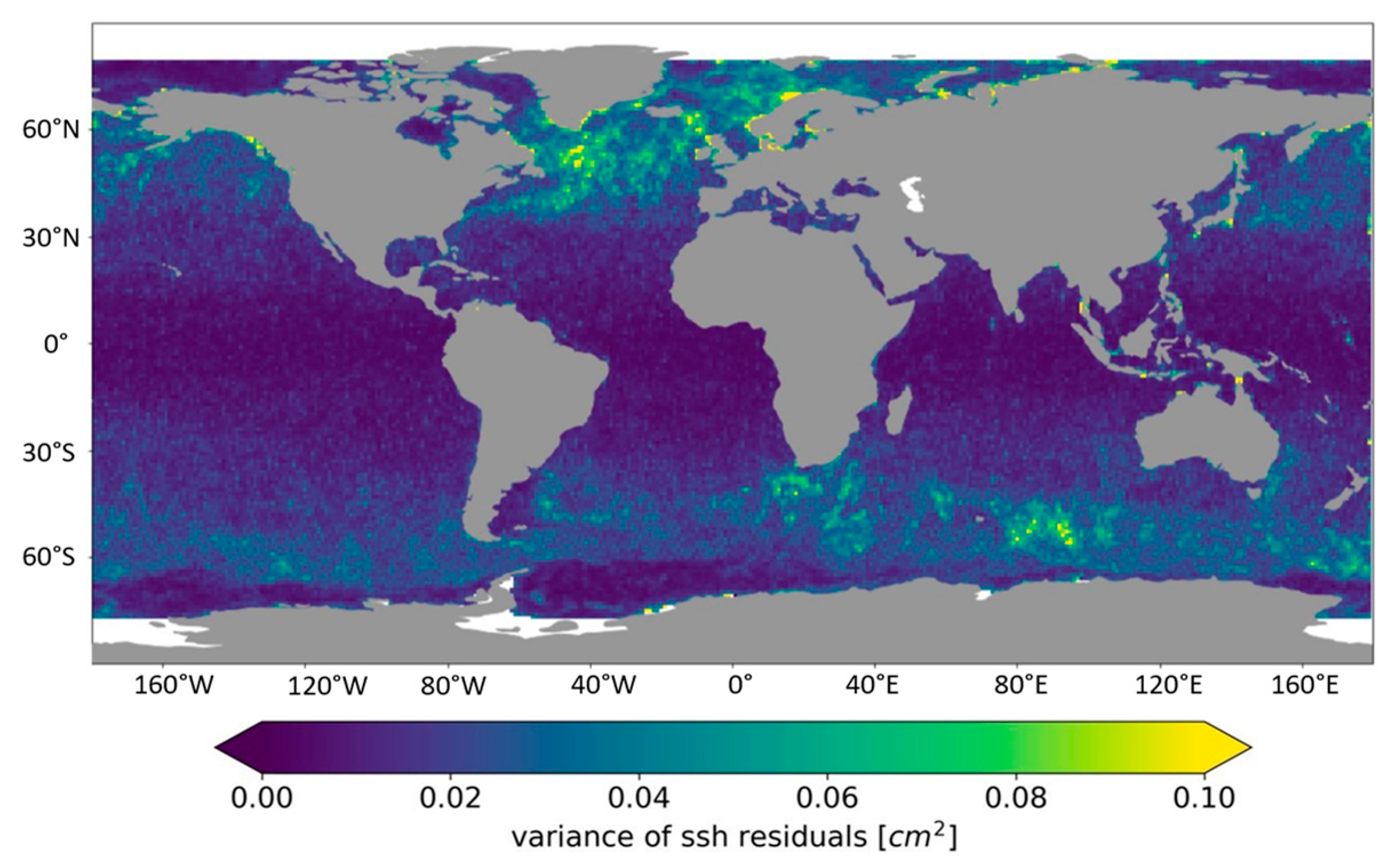
- Variance of SSH residuals: ;
- Resolved scale corresponding to the Signal-to-Noise-Ratio (SNR) equals to i.e., [34];
- KaRIn noise reduction: (in dB).
4. Results
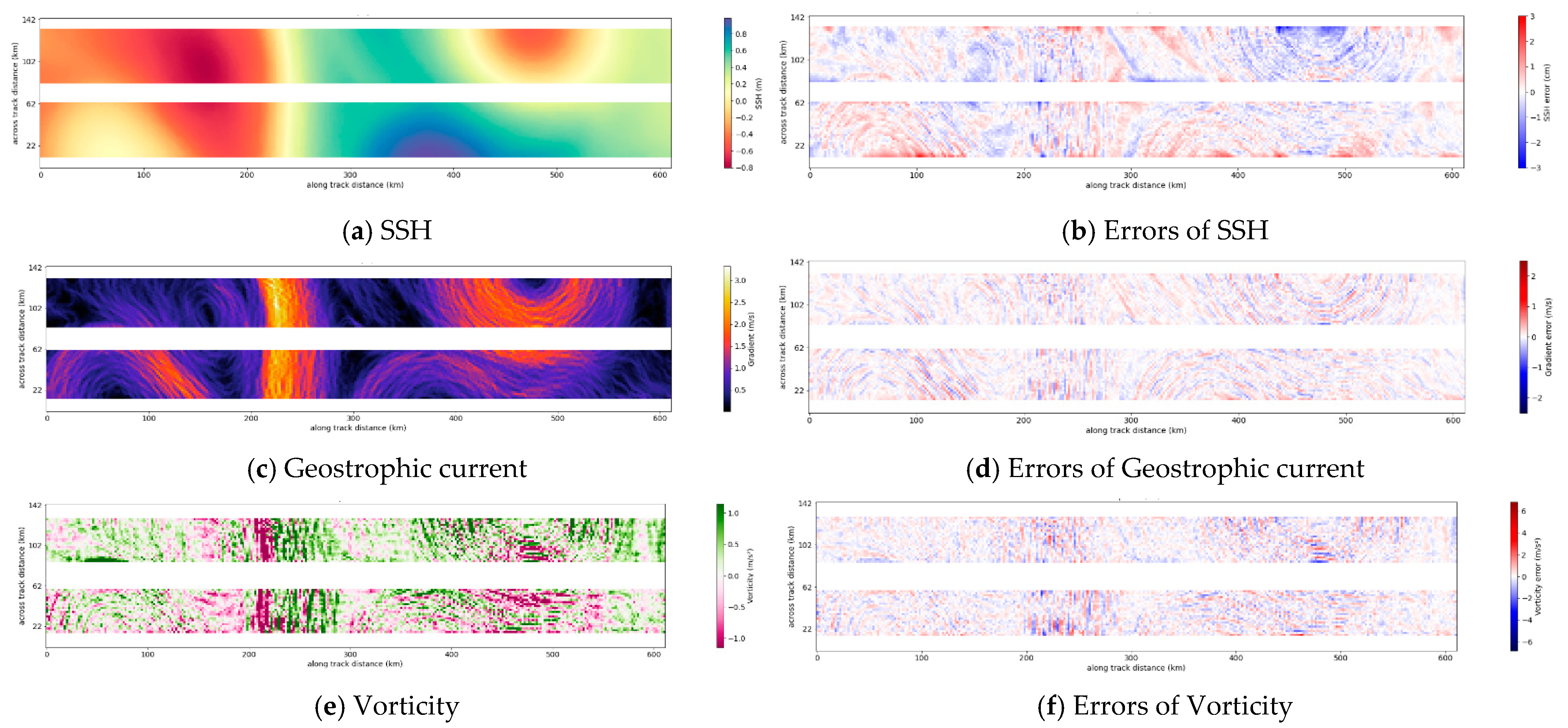
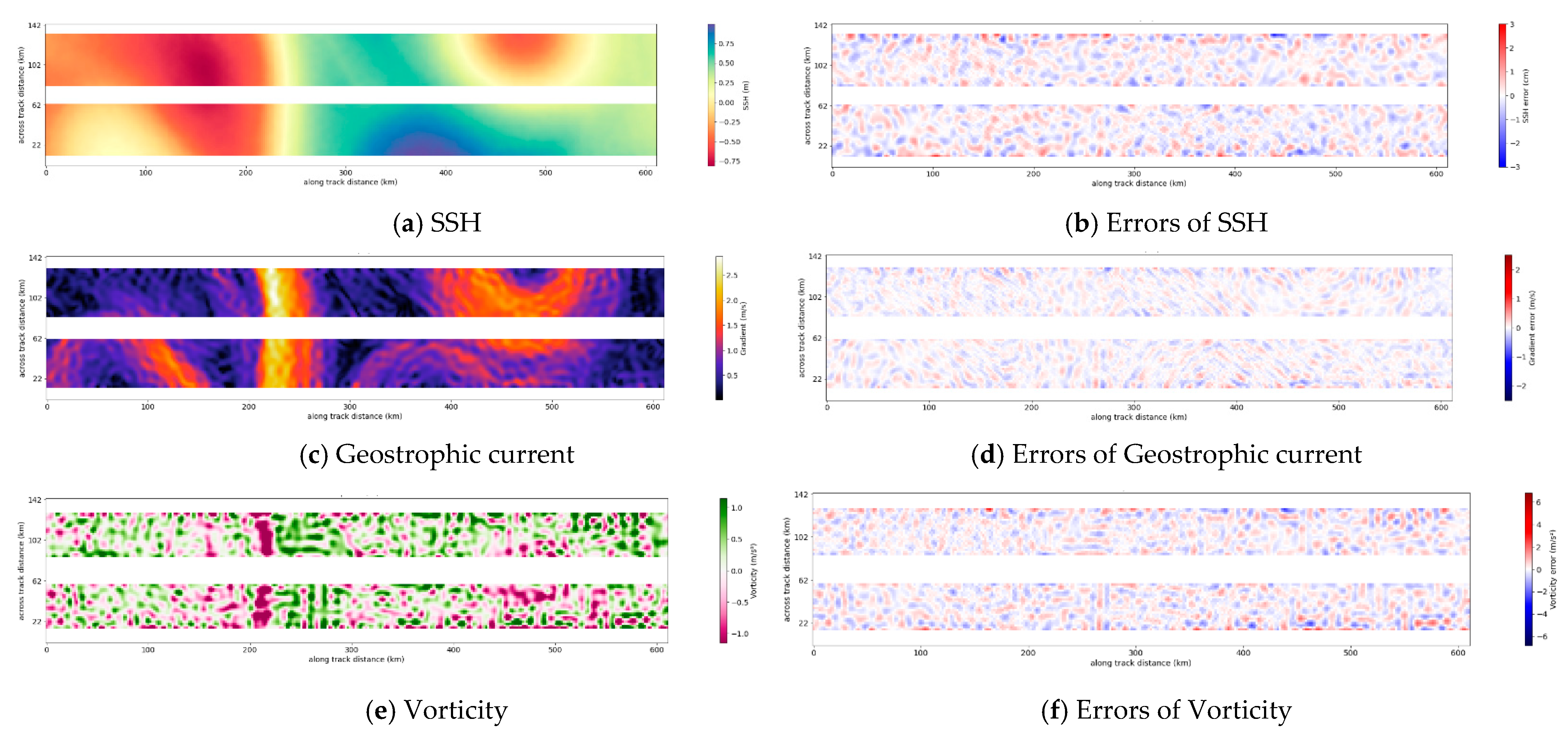
4.1. Examples of Denoised Swaths
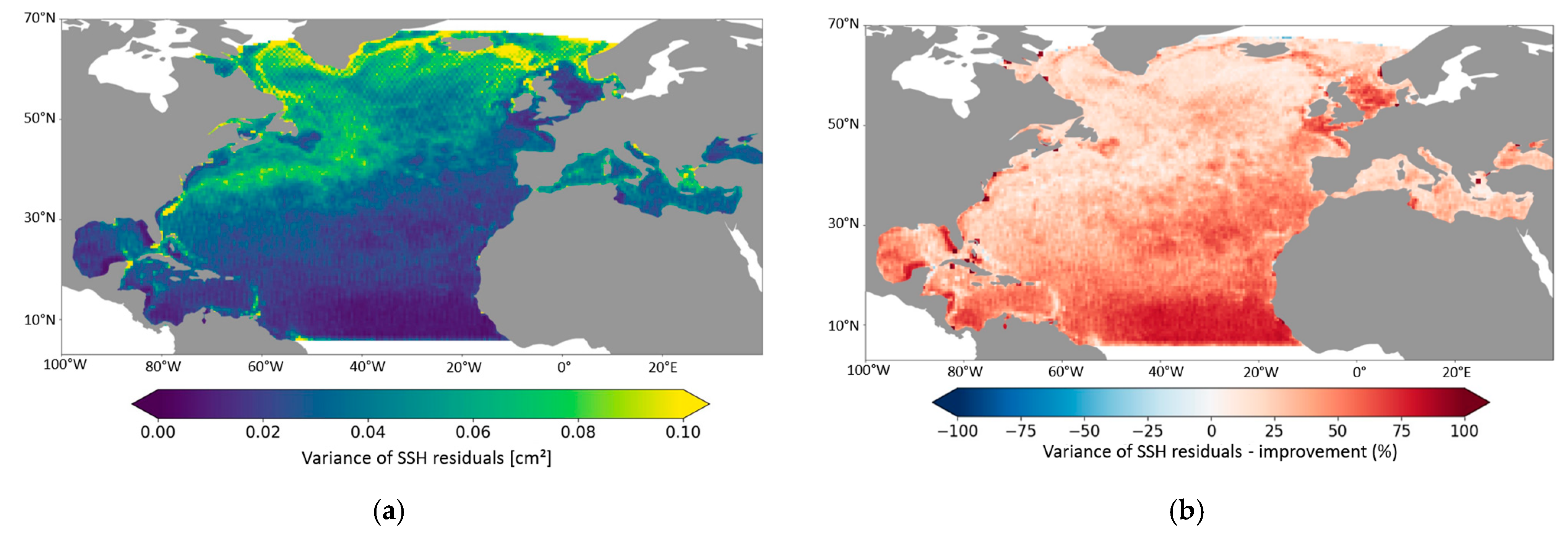
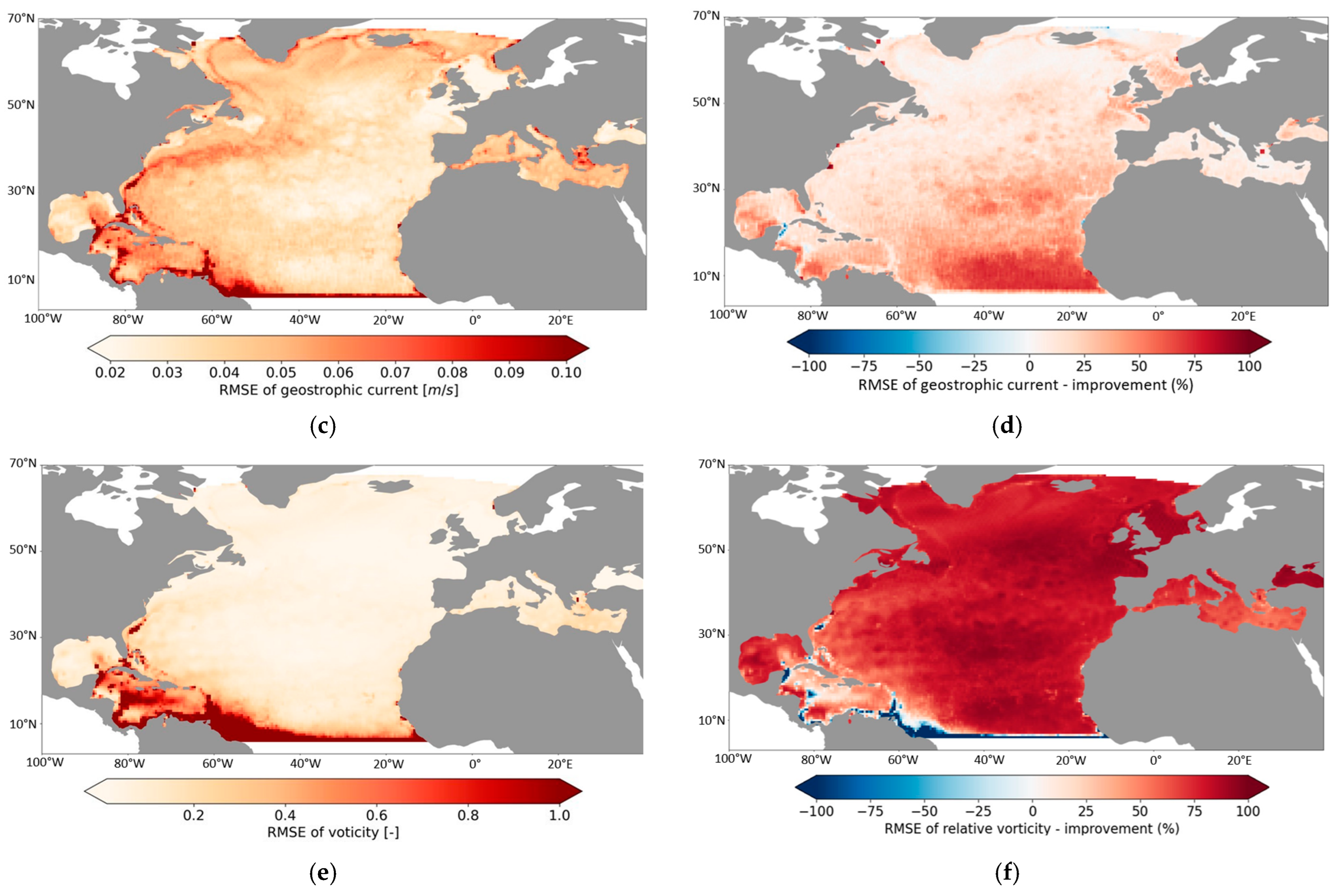
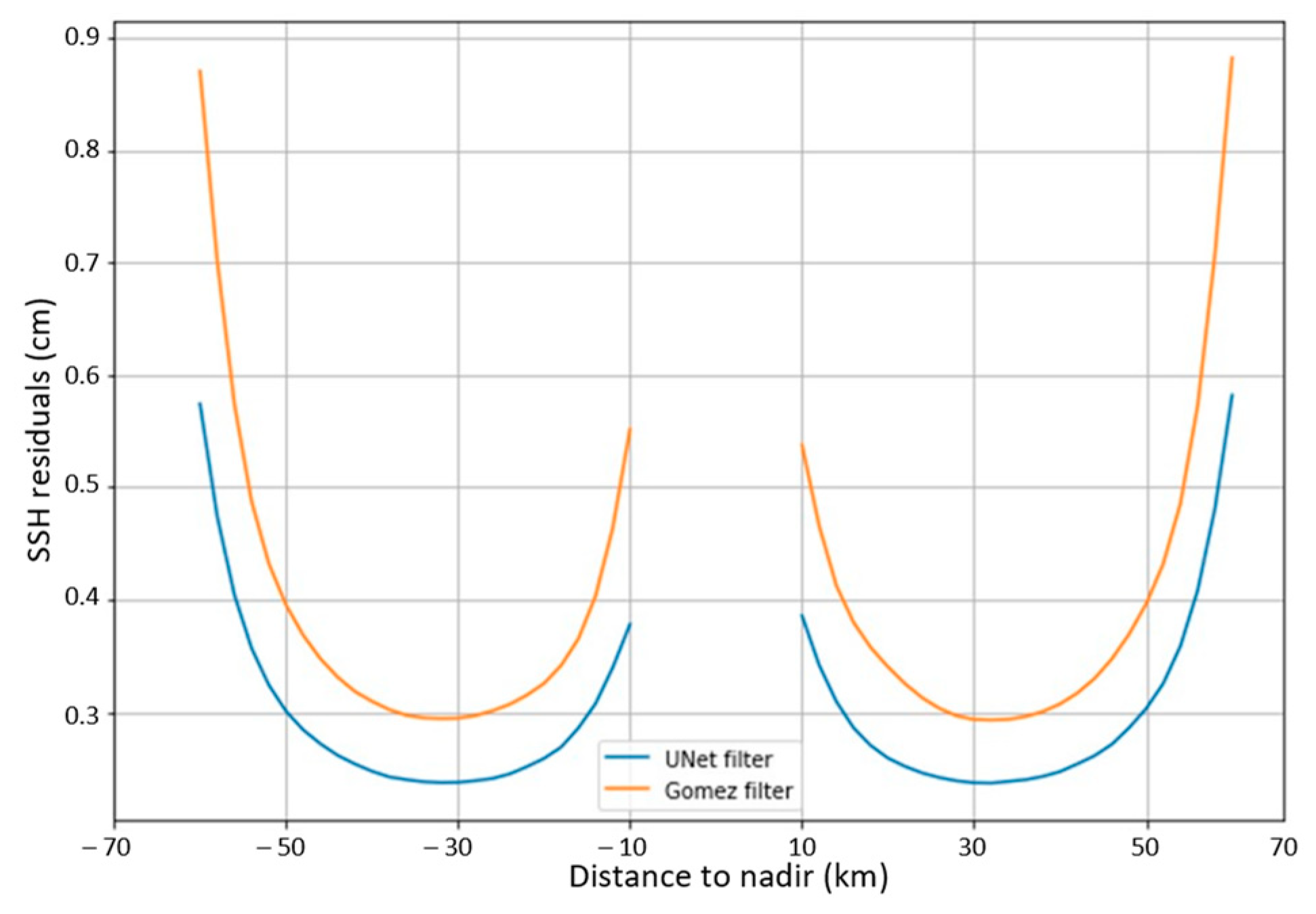
4.2. Statistics and Geographical Variations
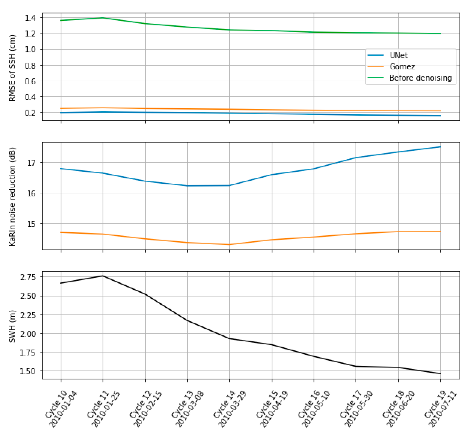
4.3. Temporal Scores
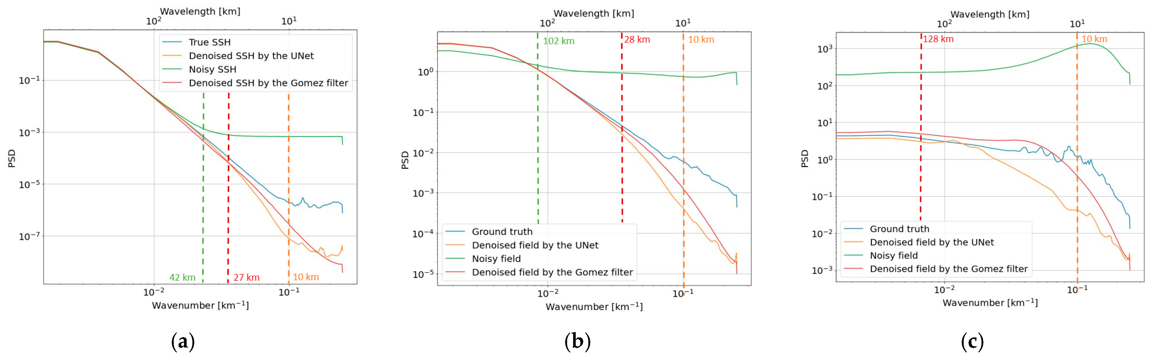
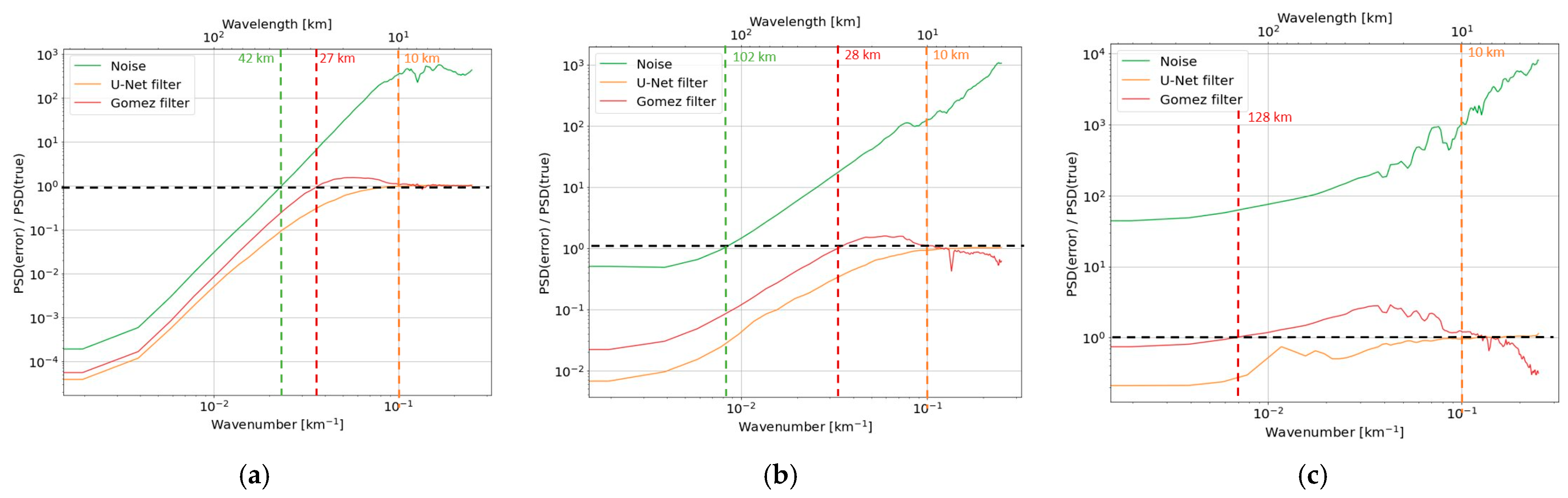
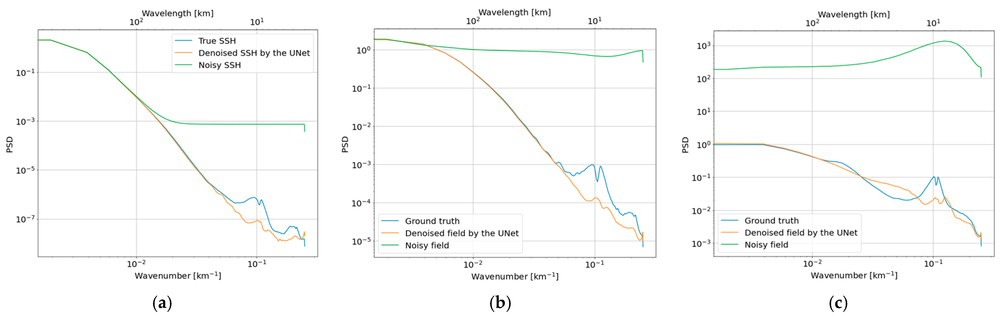
4.4. Spectral Analysis
5. Robustness of the Model
5.1. Method Applied to Test the Robustness
- A new dataset is generated either with the modified KaRIn noise or with another ocean model. As before, the year 2010 is used. The objective of this step is to simulate data which would have different properties from those of the SWOT simulator.
- When the real SWOT data are available, the ground truth will not be accessible. Thus, the U-Net is applied in inference on this new dataset without training.
- The scores are calculated from the output of the model.
5.2. Scenario: 50% More Noise
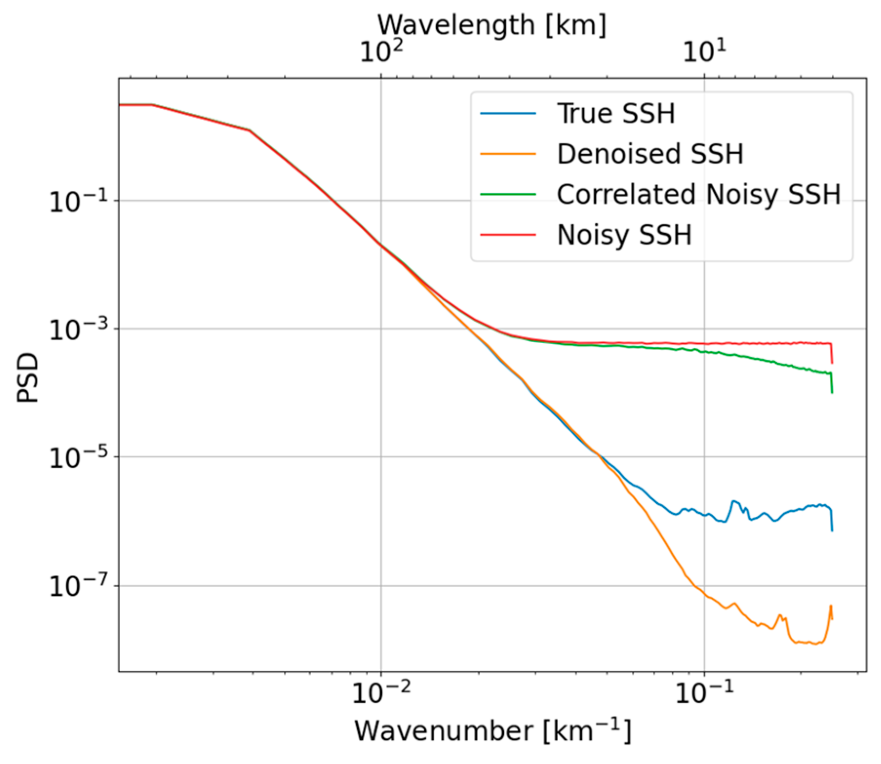
5.3. Scenario: Correlated Noise
5.3.1. Generation of the Correlated Noise
5.3.2. Results
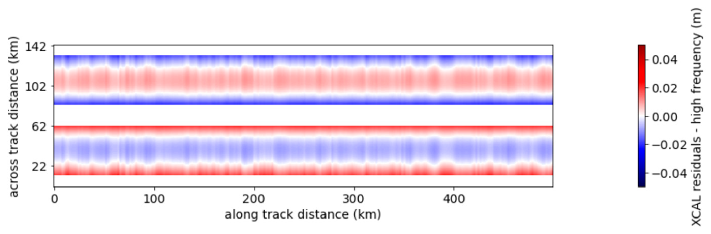
5.4. Scenario: XCal Residuals
5.4.1. XCal Residuals
5.4.2. Results
5.5. Generalization of the Model
5.5.1. Glorys Ocean Model
5.5.2. Results
5.6. Discussion about the Robustness of the U-Net
6. Interpretation of De-Noised Ocean Dynamics
7. Conclusions
Author Contributions
Funding
Acknowledgments
Conflicts of Interest
Appendix A


Appendix B

| No Filter | Without Retraining | With Retraining | |
|---|---|---|---|
| RMSE (cm) | 1.91 | 0.24 | 0.20 |
| Mean of SSH residuals (mm) | <0.1 | <0.1 | <0.1 |
| Variance of SSH residuals (cm2) | 3.67 | 0.06 | 0.04 |
| RMSEV (m/s) | 1.22 | 0.05 | 0.04 |
| RMSEζ (-) | 15.75 | 0.40 | 0.35 |
| Resolved scale of SSH (km) | 56 | 10 | 10 |
| Resolved scale of V (km) | >1000 | 10 | 10 |
| Resolved scale of ζ (km) | >1000 | 10 | 10 |
References
- Gómez-Navarro, L.; Cosme, E.; Le Sommer, J.; Papadakis, N.; Pascual, A. Development of an Image De-Noising Method in Preparation for the Surface Water and Ocean Topography Satellite Mission. Remote Sens. 2020, 12, 734. [Google Scholar] [CrossRef]
- Morrow, R.; Fu, L.-L.; Ardhuin, F.; Benkiran, M.; Chapron, B.; Cosme, E.; D’ovidio, F.; Farrar, J.T.; Gille, S.T.; Lapeyre, G.; et al. Global Observations of Fine-Scale Ocean Surface Topography with the Surface Water and Ocean Topography (SWOT) Mission. Front. Mar. Sci. 2019, 6, 232. [Google Scholar] [CrossRef]
- Fu, L.-L.; Alsdorf, D.; Morrow, R.; Rodriguez, E.; Mognard, N. SWOT: The Surface Water and Ocean Topography Mission; JPL Publication 12-05; JPL: Pasadena, CA, USA, 2012; p. 228.
- Durand, M.; Fu, L.-L.; Lettenmaier, D.P.; Alsdorf, D.E.; Rodriguez, E.; Esteban-Fernandez, D. The Surface Water and Ocean Topography Mission: Observing Terrestrial Surface Water and Oceanic Submesoscale Eddies. Proc. IEEE 2010, 98, 766–779. [Google Scholar] [CrossRef]
- Fu, L.-L.; Ubelmann, C. On the Transition from Profile Altimeter to Swath Altimeter for Observing Global Ocean Surface Topography. J. Atmos. Ocean Technol. 2014, 31, 560–568. [Google Scholar] [CrossRef]
- Fu, L.-L. SWOT Science Requirements Document; JPL Publication D-61923; JPL: Pasadena, CA, USA, 2018; p. 29.
- Esteban-Fernandez, D. SWOT Project Mission Performance and Error Budget 2014. Available online: https://swot.jpl.nasa.gov/system/documents/files/2178_2178_SWOT_D-79084_v10Y_FINAL_REVA__06082017.pdf (accessed on 7 April 2023).
- Gaultier, L.; Ubelmann, C.; Fu, L.-L. The Challenge of Using Future SWOT Data for Oceanic Field Reconstruction. J. Atmos. Ocean. Technol. 2016, 33, 119–126. [Google Scholar] [CrossRef]
- Chelton, D.B.; Samelson, R.M.; Farrar, J.T. The Effects of Uncorrelated Measurement Noise on SWOT Estimates of Sea-Surface Height, Velocity and Vorticity. J. Atmos. Ocean. Technol. 2022, 39, 72. [Google Scholar] [CrossRef]
- Gómez-Navarro, L.; Fablet, R.; Mason, E.; Pascual, A.; Mourre, B.; Cosme, E.; Le Sommer, J. SWOT Spatial Scales in the Western Mediterranean Sea Derived from Pseudo-Observations and an Ad Hoc Filtering. Remote Sens. 2018, 10, 599. [Google Scholar] [CrossRef]
- Fan, L.; Zhang, F.; Fan, H.; Zhang, C. Brief review of image denoising techniques. Vis. Comput. Ind. Biomed. Art 2019, 2, 1–12. [Google Scholar] [CrossRef]
- Ilesanmi, A.E.; Ilesanmi, T.O. Methods for image denoising using convolutional neural network: A review. Complex Intell. Syst. 2021, 7, 2179–2198. [Google Scholar] [CrossRef]
- Tian, C.; Fei, L.; Zheng, W.; Xu, Y.; Zuo, W.; Lin, C.-W. Deep learning on image denoising: An overview. Neural Netw. 2020, 131, 251–275. [Google Scholar] [CrossRef]
- Krizhevsky, A.; Sutskever, I.; Hinton, G.E. Imagenet classification with deep convolutional neural networks. Commun. ACM 2017, 60, 84–90. [Google Scholar] [CrossRef]
- Jifara, W.; Jiang, F.; Rho, S.; Cheng, M.; Liu, S. Medical image denoising using convolutional neural network: A residual learning approach. J. Supercomput. 2017, 75, 704–718. [Google Scholar] [CrossRef]
- Kovacs, A.; Bukki, T.; Legradi, G.; Meszaros, N.J.; Kovacs, G.Z.; Prajczer, P.; Tamaga, I.; Seress, Z.; Kiszler, G.; Forgacs, A.; et al. Robustness analysis of denoising neural networks for bone scintigraphy. Nucl. Instrum. Methods Phys. Res. Sect. A Accel. Spectrometers Detect. Assoc. Equip. 2022, 1039, 167003. [Google Scholar] [CrossRef]
- Wang, P.; Zhang, H.; Patel, V.M. SAR Image Despeckling Using a Convolutional Neural Network. IEEE Signal Process. Lett. 2017, 24, 1763–1767. [Google Scholar] [CrossRef]
- Carrere, L.; Faugère, Y.; Ablain, M. Major improvement of altimetry sea level estimations using pressure-derived corrections based on ERA-Interim atmospheric reanalysis. Ocean Sci. 2016, 12, 825–842. [Google Scholar] [CrossRef]
- Brodeau, L.; Sommer, J.L.; Albert, A. Ocean-Next/eNATL60: Material Describing the Set-Up and the Assessment of NEMO-eNATL60 Simulations; Zenodo: Geneva, Switzerland, 2020. [Google Scholar] [CrossRef]
- Ajayi, A.; Le Sommer, J.; Chassignet, E.; Molines, J.; Xu, X.; Albert, A.; Cosme, E. Spatial and Temporal Variability of the North Atlantic Eddy Field From Two Kilometric-Resolution Ocean Models. J. Geophys. Res. Ocean. 2020, 125, e2019JC015827. [Google Scholar] [CrossRef]
- Li, Z.; Liu, F.; Yang, W.; Peng, S.; Zhou, J. A Survey of Convolutional Neural Networks: Analysis, Applications, and Prospects. IEEE Trans. Neural Netw. Learn. Syst. 2021, 33, 6999–7019. [Google Scholar] [CrossRef]
- Albawi, S.; Mohammed, T.A.; Al-Zawi, S. Understanding of a convolutional neural network. In Proceedings of the 2017 International Conference on Engineering and Technology (ICET), Antalya, Turkey, 21–23 August 2017; pp. 1–6. [Google Scholar] [CrossRef]
- Vincent, P.; Larochelle, H.; Lajoie, I.; Bengio, Y.; Manzagol, P.-A. Stacked Denoising Autoencoders: Learning Useful Representations in a Deep Network with a Local Denoising Criterion. J. Mach. Learn. Res. 2010, 11, 3371–3408. [Google Scholar]
- Guo, X.; Liu, X.; Zhu, E.; Yin, J. Deep Clustering with Convolutional Autoencoders. Neural Inf. Process. 2017, 10635, 373–382. [Google Scholar] [CrossRef]
- Ronneberger, O.; Fischer, P.; Brox, T. U-Net: Convolutional networks for biomedical image segmentation. In Medical Image Computing and Computer-Assisted Intervention 2015; Navab, N., Hornegger, J., Wells, W.M., Frangi, A.F., Eds.; Springer International Publishing: Cham, Switzerland, 2015; pp. 234–241. [Google Scholar]
- Komatsu, R.; Gonsalves, T. Comparing U-Net Based Models for Denoising Color Images. AI 2020, 1, 465–487. [Google Scholar] [CrossRef]
- Dong, H.; Yang, G.; Liu, F.; Mo, Y.; Guo, Y. Automatic Brain Tumor Detection and Segmentation Using U-Net Based Fully Convolutional Networks. arXiv 2017, arXiv:1705.03820. [Google Scholar]
- Agrawal, S.; Barrington, L.; Bromberg, C.; Burge, J.; Gazen, C.; Hickey, J. Machine Learning for Precipitation Nowcasting from Radar Images. arXiv 2019, arXiv:1912.12132. [Google Scholar]
- Zhao, H.; Gallo, O.; Frosio, I.; Kautz, J. Loss Functions for Image Restoration with Neural Networks. IEEE Trans. Comput. Imaging 2017, 3, 47–57. [Google Scholar] [CrossRef]
- Taylor, V.; Nitschke, G. Improving Deep Learning using Generic Data Augmentation. arXiv 2017, arXiv:1708.06020. [Google Scholar]
- Paszke, A.; Gross, S.; Massa, F.; Lerer, A.; Bradbury, J.; Chanan, G.; Killeen, T.; Lin, Z.; Gimelshein, N.; Antiga, L.; et al. PyTorch: An Imperative Style, High-Performance Deep Learning Library. arXiv 2019, arXiv:1912.01703. [Google Scholar]
- Kingma, D.P.; Ba, J. Adam: A Method for Stochastic Optimization. arXiv 2017, arXiv:1412.6980. [Google Scholar]
- Akiba, T.; Sano, S.; Yanase, T.; Ohta, T.; Koyama, M. Optuna. A Next-generation Hyperparameter Optimization Framework. In Proceedings of the 25th ACM SIGKDD International Conference on Knowledge Discovery & Data Mining, Anchorage, AK, USA, 25 July 2019; pp. 2623–2631. [Google Scholar] [CrossRef]
- Wang, J.; Fu, L.-L.; Torres, H.S.; Chen, S.; Qiu, B.; Menemenlis, D. On the Spatial Scales to be Resolved by the Surface Water and Ocean Topography Ka-Band Radar Interferometer. J. Atmos. Ocean Technol. 2019, 36, 87–99. [Google Scholar] [CrossRef]
- Dufau, C.; Orsztynowicz, M.; Dibarboure, G.; Morrow, R.; Le Traon, P.-Y. Mesoscale resolution capability of altimetry: Present and future. J. Geophys. Res. Ocean. 2016, 121, 4910–4927. [Google Scholar] [CrossRef]
- Stiles, B.; Dubois. Algorithm Theoretical Basis Document for the Level 2 LR Sea Surface Height Science Algorithm. Technical Note Ref JPL-D56407 Press. 2022. Available online: https://podaac-tools.jpl.nasa.gov/drive/files/misc/web/misc/swot_mission_docs/pdd/D-56407_SWOT_Product_Description_L2_LR_SSH_20220902_RevA.pdf (accessed on 7 April 2023).
- Molero, B.; Bohe, A.; Dubois, P. From 250 m to 2 km Posting: Implications of the L2B Averaging Step (Presented in the SWOT Meeting). 2022. Available online: https://swotst.aviso.altimetry.fr/programs/2022-swot-st-program (accessed on 7 April 2023).
- Dibarboure, G.; Ubelmann, C.; Flamant, B.; Briol, F.; Peral, E.; Bracher, G.; Vergara, O.; Faugère, Y.; Soulat, F.; Picot, N. Data-Driven Calibration Algorithm and Pre-Launch Performance Simulations for the SWOT Mission. Remote Sens. 2022, 14, 6070. [Google Scholar] [CrossRef]
- Jean-Michel, L.; Eric, G.; Romain, B.-B.; Gilles, G.; Angélique, M.; Marie, D.; Clément, B.; Mathieu, H.; Olivier, L.G.; Charly, R.; et al. The Copernicus Global 1/12° Oceanic and Sea Ice GLORYS12 Reanalysis. Front. Earth Sci. 2021, 9. [Google Scholar] [CrossRef]
- Callies, J.; Ferrari, R.; Klymak, J.M.; Gula, J. Seasonality in submesoscale turbulence. Nat. Commun. 2015, 6, 6862. [Google Scholar] [CrossRef] [PubMed]
- Richman, J.G.; Arbic, B.K.; Shriver, J.F.; Metzger, E.J.; Wallcraft, A.J. Inferring dynamics from the wavenumber spectra of an eddying global ocean model with embedded tides. J. Geophys. Res. Atmos. 2012, 117, C12012. [Google Scholar] [CrossRef]
- Sasaki, H.; Klein, P.; Qiu, B.; Sasai, Y. Impact of oceanic-scale interactions on the seasonal modulation of ocean dynamics by the atmosphere. Nat. Commun. 2014, 5, 5636. [Google Scholar] [CrossRef] [PubMed]
- Su, Z.; Wang, J.; Klein, P.; Thompson, A.F.; Menemenlis, D. Ocean submesoscales as a key component of the global heat budget. Nat. Commun. 2018, 9, 1–8. [Google Scholar] [CrossRef] [PubMed]
- Ferrari, R.; Wunsch, C. Ocean Circulation Kinetic Energy: Reservoirs, Sources, and Sinks. Annu. Rev. Fluid Mech. 2009, 41, 253–282. [Google Scholar] [CrossRef]
- Renault, L.; Marchesiello, P.; Masson, S.; McWilliams, J.C. Remarkable Control of Western Boundary Currents by Eddy Killing a Mechanical Air-Sea Coupling Process. Geophys. Res. Lett. 2019, 46, 2743–2751. [Google Scholar] [CrossRef]
- Qiu, B.; Chen, S.; Klein, P.; Torres, H.; Wang, J.; Fu, L.-L.; Menemenlis, D. Reconstructing Upper-Ocean Vertical Velocity Field from Sea Surface Height in the Presence of Unbalanced Motion. J. Phys. Oceanogr. 2020, 50, 55–79. [Google Scholar] [CrossRef]
- Siegelman, L.; Klein, P.; Rivière, P.; Thompson, A.F.; Torres, H.S.; Flexas, M.; Menemenlis, D. Enhanced upward heat transport at deep submesoscale ocean fronts. Nat. Geosci. 2019, 13, 50–55. [Google Scholar] [CrossRef]
- Zhang, K.; Zuo, W.; Chen, Y.; Meng, D.; Zhang, L. Beyond a Gaussian Denoiser: Residual Learning of Deep CNN for Image Denoising. IEEE Trans. Image Process. 2017, 26, 3142–3155. [Google Scholar] [CrossRef]


| U-Net | Gomez Filter | Median Filter | Lanczos Smoother | No Filter | |
|---|---|---|---|---|---|
| RMSESSH (cm) | 0.19 | 0.24 | 0.31 | 0.44 | 1.27 |
| KaRIn noise reduction | 45 (16 dB) | 28 (14 dB) | 17 (12 dB) | 8 (9 dB) | - |
| Mean of SSH residuals (mm) | <0.1 | <0.1 | <0.1 | <0.1 | 0. |
| Variance of SSH residuals (cm2) | 0.04 | 0.07 | 0.10 | 0.20 | 1.63 |
| RMSEV (m/s) | 0.04 | 0.06 | 0.10 | 0.17 | 0.78 |
| RMSEζ (-) | 0.37 | 0.53 | 1.11 | 2.07 | 10.50 |
| U-Net | Gomez Filter | Median Filter | Lanczos Smoother | No Filter | |
|---|---|---|---|---|---|
| RMSESSH (cm) | 0.32 | 0.84 | 0.87 | 0.81 | 1.21 |
| KaRIn noise reduction | 14 (11 dB) | 2 (3 dB) | 2 (3 dB) | 2 (3 dB) | - |
| Mean of SSH residuals (cm) | 0.01 | 0.04 | 0.03 | 0.01 | <0.01 |
| RMSEV (m/s) | 0.09 | 0.14 | 0.14 | 0.21 | 0.69 |
| RMSEζ (-) | 0.67 | 0.80 | 1.10 | 1.88 | 7.92 |
| 50% More Noise | Correlated Noise | XCal Residuals | Glorys Data | |||||
|---|---|---|---|---|---|---|---|---|
| No Filter | U-Net | No Filter | U-Net | No Filter | U-Net | No Filter | U-Net | |
| RMSE (cm) | 1.91 | 0.24 | 0.97 | 0.20 | 1.65 | 0.91 | 1.33 | 0.13 |
| Mean of SSH residuals (mm) | <0.1 | <0.1 | <0.1 | <0.1 | <0.1 | <0.1 | <0.1 | <0.1 |
| Variance of SSH residuals (cm2) | 3.67 | 0.06 | 0.94 | 0.04 | 2.78 | 0.81 | 1.83 | 0.02 |
| RMSEV (m/s) | 1.22 | 0.05 | 0.60 | 0.04 | 0.85 | 0.13 | 0.84 * | 0.02 * |
| RMSEζ (-) | 15.75 | 0.40 | 8.35 | 0.39 | 10.82 | 0.58 | 11.72 * | 0.12 * |
| Resolved scale of SSH (km) | 56 | 10 | 42 | 22 | 46 | 10 | 57 | 22 |
| Resolved scale of V (km) | >1000 | 10 | 102 | 20 | 171 | 10 | >1000 * | 21 * |
| Resolved scale of ζ (km) | >1000 | 10 | >1000 | 85 | >1000 | >1000 | >1000 * | 46 * |
Disclaimer/Publisher’s Note: The statements, opinions and data contained in all publications are solely those of the individual author(s) and contributor(s) and not of MDPI and/or the editor(s). MDPI and/or the editor(s) disclaim responsibility for any injury to people or property resulting from any ideas, methods, instructions or products referred to in the content. |
© 2023 by the authors. Licensee MDPI, Basel, Switzerland. This article is an open access article distributed under the terms and conditions of the Creative Commons Attribution (CC BY) license (https://creativecommons.org/licenses/by/4.0/).
Share and Cite
Tréboutte, A.; Carli, E.; Ballarotta, M.; Carpentier, B.; Faugère, Y.; Dibarboure, G. KaRIn Noise Reduction Using a Convolutional Neural Network for the SWOT Ocean Products. Remote Sens. 2023, 15, 2183. https://doi.org/10.3390/rs15082183
Tréboutte A, Carli E, Ballarotta M, Carpentier B, Faugère Y, Dibarboure G. KaRIn Noise Reduction Using a Convolutional Neural Network for the SWOT Ocean Products. Remote Sensing. 2023; 15(8):2183. https://doi.org/10.3390/rs15082183
Chicago/Turabian StyleTréboutte, Anaëlle, Elisa Carli, Maxime Ballarotta, Benjamin Carpentier, Yannice Faugère, and Gérald Dibarboure. 2023. "KaRIn Noise Reduction Using a Convolutional Neural Network for the SWOT Ocean Products" Remote Sensing 15, no. 8: 2183. https://doi.org/10.3390/rs15082183