1. Introduction
The global navigation satellite system reflectometry (GNSS-R) field has been an active focus of many investigations for around 24 years, ever since the concept was demonstrated for the first time in 1998 through an airborne experiment [
1]. The field exploded around 2014 with the first of such satellites being launched, allowing for the development of global applications of this technology. The increased resources and interest available to this research, and the formation of teams to support recent satellite missions, led to a growth in knowledge and expertise in the field. Many have since contributed to the expansion of knowledge in this field, including those based in academia, research laboratories and industry.
The following two figures provide an overview of the time evolution of the number of GNSS-R publications. Firstly, in
Figure 1, we show the increase in publications per year and the relationship to the total amount of publications in the general remote sensing field. General remote sensing includes radiometry, radar, synthetic aperture radar, optical sensors, spectral sensors, and all sciences from areas of atmospheric and land monitoring, as illustrated in
Figure 1. GNSS-R publications have seen a steep increase in the recent years as compared to the overall increase in all remote sensing publications. GNSS-R publications are beginning to account for nearly 1% of all remote sensing publications.
GNSS-R publications are distributed as follows: 260 publications in IEEE journals, 160 publications in MDPI, out of which 43 were published in the MDPI Special Issue series “Applications of GNSS Reflectometry for Earth Observation I, II and III” (e.g., 27% of all MDPI publications), 43 publications by Elsevier, 30 publications by Springer Nature, and 28 publications by American Geophysical Union Publications. The data were collected from the Clarivate Web of Science Core Collection using the keywords “remote sensing and (reflectometry GNSS or GNSS-R or GNSS-IR)”.
Figure 2 shows the distribution of GNSS-R-related publications per major region or continent, applying the Clarivate Web of Science Core Collection “core country/region metric”. The large majority of publications for GNSS-R have been written by researchers based in Europe, Asia and North America, with 49.71%, 27.61% and 19.88% of all publications, respectively. Fewer publications have been produced by those based in South America, Africa and Oceania which account for the remaining 2.8%.
GNSS-R is a bistatic radar technique based on signals of opportunity. The transmitted signal is sent by a GNSS satellite; then, the signal scatters off the Earth’s surface and is received by a GNSS receiver. The GNSS receiver can be placed on a ground-based instrument, on an aircraft, on a satellite or on a constellation of satellites. Each platform provides different capabilities in terms of spatial and temporal resolution. Generally speaking, a ground-based platform can offer high-resolution data, but its coverage is limited to a very small area within the static antenna beam. An airborne platform provides a medium spatial resolution in the order of 300 m to 1 km, depending on the flight height, and potentially provides regional spatial coverage in the order of 100′s of kilometers. A satellite platform provide global coverage, which depends on the selected orbit, and the spatial resolution ranges from 1 km to hundreds of kilometers, being set primarily by the scattering properties of the surface under observation. For example, sea ice will be observed at 1 km spatial resolutions, while ocean surface will be observed at > 25 km spatial resolutions.
Figure 3 provides an illustration of the remote sensing platforms used for GNSS-R instruments.
As the GNSS signal is scattered from the Earth’s surface, it is affected by its characteristics. For example, over the ocean, the contribution of an area of scattering increases or decreases as the ocean is rougher or calmer. Over the land, there are many geophysical parameters that can affect signals. The reflected GNSS signal is affected by the surface roughness of the scene as well as the water content of the soil since the moisture content of the soil changes the dielectric properties of the surface. Although the GNSS-L-band signal can penetrate vegetation, the water content of the plants, as well as the density and height, impacts the signal due to volume scattering. GNSS signals are sensitive to standing water, such as lakes, rivers, or wetlands, and also to water in a frozen state, such as frozen soil (during winter) or sea ice. Reflections on calm water and ice produce coherent reflections as compared to reflections from bare soil or vegetated soil. The ability to detect inland water is valuable for mapping inundation in wetlands or other floods. GNSS reflections can also be used for frozen soil detection, which allows for studies of the freeze/thaw characteristics of land surfaces.
Thanks to its sensitivity to different surfaces, GNSS-R signals can be used in many different applications.
Figure 4 shows an image relating the GNSS-R applications to the essential climate variables (ECV) described by the global climate observing system (GCOS), providing a clear idea as to the relevance of the GNSS-R field to improving our knowledge of Earth and its processes.
The power collected by a GNSS receiver after the GNSS signal scatters over the Earth’s surface is known as a delay–Doppler map (DDM). The mathematical equation was defined in [
2,
3] and can easily be found in the literature. We provide the equations for the general understanding of the different studies that are explained here and for the completeness of this review article. Equation (1) describes the reflected GNSS signal that would be received from a surface dominated by incoherent scattering.
where:
identifies the various surface pixels in the scattering area;
represents the coherent integration time;
stands for GPS transmitted power;
and denote the transmitter and receiver antenna gain, respectively;
is the wavelength of the GPS signal (which is 24.42 cm at GPS-L2C);
and represent the distance from the transmitter to the particular surface pixel , and the distance between the receiver and the particular surface pixel , respectively;
The sinc() function characterizes the signal spread in Doppler;
The delta function characterizes the spread of the signal in time;
The bistatic radar cross section of a rough surface is given by the following equation: , where is the Fresnel reflection coefficient, is the probability density function of the surface slopes, and and are the tangential and perpendicular components of the bisector vector or scattering vector .
Comparatively, Equation (2) describes the reflected GNSS signal that would be received from a surface dominated by coherent scattering.
where:
corresponds to the surface specular point;
is the averaged reflection coefficient at . This is computed from evaluating the scattering surface average reflection coefficient at the specular direction by performing .
To illustrate the different types of scattering we provide in
Figure 5 the different types of scattering and the corresponding DDMs that are characteristic of different types of surfaces.
The following sections review the different aspects of the GNSS-R field.
Section 2 reviews the technology advancements in the field, providing first a review of the evolution since it was first proposed in 1988.
Section 3 covers the advancements specific to ocean applications.
Section 4 covers the advancements specific to land applications.
Section 5 is dedicated to describing the applications on the Earth’s cryosphere;
Section 6 provides insight into novel applications derived from GNSS-R, but which are not specifically part of the ocean, land, or cryosphere.
Section 7 provides a discussion on where the GNSS-R field seems to be heading in the near future. Finally, conclusions are presented in
Section 8.
2. Technology Advancements
GNSS-R was proposed in the late 1980s as a multi-static scatterometer [
4], and a few years later, in 1993, the interferometric GNSS-R technique (iGNSS-R) [
5] was proposed for use in sea altimetry. This technique was based on the cross correlation of the direct and reflected signals and makes use of the large-bandwidth military codes for a high-precision opportunistic altimeter. Three years after that, the most broadly used technique, known as conventional GNSS-R (cGNSS-R), was proposed by Katzberg and Garrison [
6]. It was not until 1998 that the GNSS-R concept was demonstrated [
1] from an airborne platform. The technology used at that time consisted of a commercial GPS receiver from GEC Plessey semiconductors, which was modified to include an open-loop correlator at different delay lags from the peak point position. In this case, the antenna used was a single left-hand circularly polarized (LHCP) down-looking antenna. Besides iGNSS-R and cGNSS-R, which tend to be used for airborne and spaceborne platforms, a ground-based monitoring technique was also conceived of for remote sensing applications. This is called GNSS interferometric reflectometry (GNSS-IR) [
7]. This technique is based on a geodetic GNSS receiver that receives a combination of both the direct and reflected signal, causing an interference pattern in the observed signal which can be used to estimate land-related properties. In this section, the latest technology advances in the last 10 years in the GNSS-R and GNSS-IR field will be covered, including the use of spaceborne and airborne receivers for GNSS-R cases and ground-based receivers for GNSS-IR cases.
2.1. Ground-Based Receivers
This category of technological advancements is devoted to ground-based sensors. Early in the 2010s, the GNSS-IR technique was conceived independently in [
7,
8]. Since then, geodetic GNSS receivers have been used to estimate soil moisture or vegetation properties. However, since commercial geodetic receivers are used for GNSS-IR, most advances have come from new algorithms [
9] and not from new receivers or technologies. Despite that, it is worth mentioning that new applications have been derived using the GNSS-IR concept. Sea level was monitored using the GNSS-IR concept [
10], lake ice thickness was retrieved for the first time in [
11], and sea ice and snow thicknesses were also retrieved using multi-frequency observations and using a four-layer scattering model [
12].
The second technique covered in this section is a new technological approach that makes use of the scattered GNSS-R signals in order to generate a synthetic aperture radar (SAR)-like image [
13]. The technology is based on ground-based GNSS-R receivers that accurately compute and compensate the delay and Doppler of the reflected signal of a satellite while it crosses the sky. A SAR-like processing operation can be performed, producing a 2D image of a wide area in front of the receiver [
14].
2.2. Airborne Receivers
Airborne GNSS-R receivers have been used as technology demonstrators for novel techniques and technologies. As previously stated, the first GNSS-R signal acquired by Katzberg and Garrison was retrieved from an airborne platform [
4]. The number of GNSS-R instruments that have flown in airborne campaigns is large, which was especially true before the deployment of the CYGNSS constellation. In this section, we will cover those instruments that, in recent years, have provided large technological development with respect to previous versions or actual satellite-based versions.
In chronological order, the GOLD-R instrument (2010–2014), developed by the Institut de Ciències de l’Espai/Institut Estudis Espaials de Catalunya (ICE-CSIC/IEEC) with the collaboration of UPC and ESA, was a pioneer instrument capable of working at the GPS L1 band at multiple polarizations [
15]. The basic design works by sampling up to 20 MHz of bandwidth at the GPS L1 band using a single-LHCP patch antenna. The instrument is able to work in different modes thanks to the collection of the IF samples (e.g., I/Q down-sampled data) of both the direct and the reflected signals. It was developed to show the differences between iGNSS-R and cGNSS-R processing modes [
16].
The second airborne instrument covered in this review is the global navigation satellite system reflectometry instrument (GLORI) [
17]. Designed in 2015, this airborne instrument was a novel approach and was used to perform polarimetric studies overland. It includes a dual polarization RHCP/LHCP antenna system with 7 dBic of peak gain, capable of receiving GPS L1 and L2 signals. The receiver is based on an SDR working at 4 MHz, thus providing a delay resolution of 1/4 chips at GPS L1CA. The instrument has demonstrated the differences in RHCP and LHCP signals overland in previous work [
18], being of interest for future spaceborne missions, such as HydroGNSS [
16].
The third airborne instrument with notable technological advancements is the UPC microwave interferometric reflectometer (MIR) [
19]. Designed in 2015–2018, it conducted its maiden flight in 2018. This instrument is the first GNSS-R instrument capable of providing collocated GNSS (GPS and Galileo) L1 and L5 measurements using a 21/18 dB (L1/L5) directive antenna with beamforming. The instrument had different modes of operation, including cGNSS-R and iGNSS-R, and it aimed at proving the capabilities of high-directive antennas to remove iGNSS-R cross-talk [
20]. Additionally, the instrument demonstrated, in cGNSS-R mode, the enhanced capabilities of the GPS/Galileo L5/E5 waveforms for sea state, soil moisture, vegetation, and monitoring sea altimetry [
21,
22,
23,
24].
The last airborne instrument covered in this review is the next-generation GNSS-R instrument proposed by Ruf et al. [
25]. The instrument was conceived after CYGNSS success from a set of scientists directly involved in the CYGNSS mission. The proposed instrument was designed for operation in airborne platforms. It is able to work in L1/L5 bands in both GPS and Galileo constellations. Moreover, its down-looking antenna was designed to receive both RHCP and LCHP signals. Thus, it combined characteristics from the previously presented instruments, GLORI and MIR. The instrument was deployed in mid-2021 for continuous operation in domestic aircrafts by Air New Zealand [
26].
Thanks to electronics miniaturization, low-cost GNSS-R receivers are becoming popular among the community. Studies have shown the Earth observation potential of incorporating GNSS-R receivers into commercial aircrafts [
27]. Furthermore, UAV-based GNSS-R receivers are being developed by different research centers for low-cost and high-resolution Earth monitoring [
28,
29,
30].
2.3. Spaceborne Receivers
The first GNSS-R signal received from space was captured during a calibration routine of the Space Shuttle radar imager in 2002 [
31]. Later in 2003, the first GNSS-R receiver was launched into space as part of the UK Disaster Monitoring Constellation-1 (UK-DMC-1) mission from Surrey Satellite Technology Limited (SSTL), Guildford, UK. The mission included the first GNSS-R receiver built for that purpose as a technology demonstrator. The receiver had several configurable correlators implemented in a field-programmable gate array (FPGA) that were used to correlate the different GPS satellites in view. The antenna used was a four-element patch nadir-looking antenna array, working under left-hand circular polarization (LHCP) conditions with a directivity of ~11 dB. The mission aimed to collect small portions of data to prove the feasibility of using GNSS-R to study the ocean. Following UK-DMC-1, in 2013, the UK-TDS-1 mission was conceived with an upgraded version of the SSTL GNSS-R receiver, called SGR-ReSi [
32,
33], and with the same type of antennas as in UK-DMC-1. Both instruments were using a correlation approach called zoom transform correlator, detailed in [
34], which has been the technique adopted for most GNSS-R receivers. SGR receivers were able to provide a 1/4 chip resolution for the GPS L1CA signal, with a 500 Hz spectral resolution and a moderate power consumption below 100 W. The mission was designed with a polar orbit, and it collected data all around ocean, land, and ice.
Three years later, in 2016, the National Aeronautics and Space Administration (NASA) Cyclone GNSS (CYGNSS) mission was launched, using a similar receiver configuration as the one used in the UK-TDS-1. A GNSS-R receiver, called a delay–Doppler map imager (DDMI), was conceived for the mission. It followed the same approach as SGR-ReSi in terms of correlation approach, but the mission was designed with two sets of 28°-looking LHCP antennas arrays placed on the sides of the satellite, thus ensuring a larger coverage. The DDMI provides the same resolution as the SGR-ReSi platform of 1/4 chip for the GPS L1CA signal, with a 500 Hz spectral resolution and a moderate power consumption below 60 W. Moreover, the instrument is able to provide with an IF data mode, where the raw IQ counts can also be retrieved and downloaded down to Earth using the satellite’s link. CYGNSS consists of eight microsatellites that cover mid-latitudes of ±38°, and it has demonstrated the capabilities of using moderate-cost micro-satellite constellations to perform Earth observation at better time resolutions and similar spatial and radiometric resolutions as compared with conventional satellite missions [
35,
36].
The China Aerospace Science and Technology Corporation (CASC) has also deployed the first Chinese spaceborne GNSS-R instrument: the BuFeng-1 A/B constellation [
37]. This was successfully launched into a polar orbit in 2019. The instrument for the BuFeng-1 constellation follows the same design as the SSTL SGR-ReSi and the CYGNSS DDMI and uses the same antenna configuration as the NASA CYGNSS mission, with two antennas tilted off the sides of the spacecraft. In this case, the looking angle with respect to the nadir in the BuFeng-1 case is 26°, and it was also capable of receiving L1 BeiDou signals. The power consumption of the instrument is similar to the ones previously reported of ~55 W.
More recently, the China Meteorological Administration (CMA) in 2021 launched the FY-3E mission [
38]. The receiver included in the mission is capable of providing a larger time resolution from 1/4 of a GPS L1 chip to 1/8 of a chip. The missions’ receiver has similar characteristics to the CYGNSS DDMI or the BuFeng-1 receiver, with a similar power consumption, being only able to fit into a micro-/mini-satellite. The FY-3E mission provides near real-time data with a latency of 3 h with a polar orbit.
The Universitat Politècnica de Catalunya (UPC) NanoSat-Lab has been also contributing to the technological advances of spaceborne GNSS-R instruments. Its first CubeSats mission,
3Cat-2 [
39], launched in 2016, inaugurated the first ever spaceborne dual-band polarimetric GNSS-R instrument, which had previously been tested in a balloon experiment campaign [
40]. The instrument inherited previous ground-based GNSS-R instruments developed by the university, and it comprised an open-loop and a closed-loop receiver to work in cGNSS-R, iGNSS-R, and reconstructed GNSS-R (r-GNSS-R) modes [
41]. In this case, the antenna used was different than the ones used in UK-TDS-1 or CYGNSS, and it was specifically designed for a 6U CubeSat structure. It consisted of a 6-element patch array, providing gains of up to 13 dB at L1, and up to 11.5 dB at the GPS L2 band. Moreover, as strategically designed for CubeSats, its volume, mass, and power consumption were of ~3U of a CubeSat (30 × 30 × 10 cm
3) and less than 5 kg mass, with a power consumption below 15 W. However, spaceborne data could not be retrieved from the instrument due to a satellite bus malfunction. As an evolved version of
3Cat-2, the UPC NanoSat-Lab leads the European Space Agency (ESA) FSSCat mission [
42]. The mission was launched in September 2020, and included a combined GNSS-R receiver and an L-band radiometer using software-defined radio technology (SDR) [
43], inheriting the road paved by the UPC passive advance units (PAU) concept [
44]. The instrument called flexible microwave payload-2 (FMPL-2) includes both as GNSS-R and L-band radiometer in a single unit of a CubeSat (10 × 10 × 10 cm
3), with a mass of ~1.3 kg and power consumption ~10 W. The system antenna arrangement is similar to that 3Cat-2 of a 6U patch array, but for dual frequency (GPS L1 and the radiometry L-band at 1413.5 MHz).
Another successful GNSS-R mission example, this time from a private entity source, is the Spire Global Inc. case. The company, known for its massive CubeSat GNSS radio occultation (GNSS-RO) constellation for ionospheric measurements, has recently launched several CubeSats to provide global GNSS-R measurements [
45]. In 2019 and 2020, the company launched two batches of two 3U CubeSats with GNSS-R capabilities (two in 2019, two in 2020), providing up to 20 simultaneous correlation channels [
46]. The miniaturized receiver, produced by Spire, is the outcome of years working with GNSS-RO receivers, and it provides a multi-constellation (GPS, QZSS, Galileo) capability. The antenna system is of 3 × 1 patch antennas working at LHCP with beamforming capabilities. The instrument is able to work continuously with deployable solar panels, weighing less than 5 kg [
46]. Spire Global Inc. is currently retrieving LHCP measurements at near-nadir and RHCP measurements at grazing angles, combining their GNSS-R and GNSS-RO satellites.
The next GNSS-R mission in the pipeline is the HydroGNSS mission [
47]. The mission includes the SSTL newest version of the SGR-ReSi, the SGR-ReSi-Z. This new receiver is capable of providing multi-constellation (GPS/Galileo), multi-polarization (LHCP/RHCP), and multiband (L1 and L5) GNSS-R measurements. The receiver computes real-time L0b observations (e.g., delay–Doppler maps) at L1/E1, and the L5 data are downloaded and processed following the recommendations of [
48]. In preparation for the launch of HydroGNSS, SSTL launched the DoT-1 mission in 2019 [
47] as a tech demo with which to evaluate its new satellite bus.
Last but not least, it is worth mentioning the contribution of the soil moisture active passive (SMAP) radar receiver tuned at the GPS L2C band, whose data have been termed SMAP-reflectometry [
49]. The SMAP radar receiver collects IQ data in an open-loop mode. Data are downloaded and post-processed on Earth [
49]. Despite not being specifically designed for GNSS-R, the high directive and dual linearly polarized SMAP antenna comprises a unique platform from which to study polarimetric applications of GNSS-R over land [
50,
51,
52,
53,
54,
55].
Other space mission proposals have been also developed in the recent years including iGNSS-R receivers [
56,
57], but neither mission has ever been implemented or launched.
2.4. Technology Advancement Summary
GNSS-R has been rapidly growing since 2013 UK-TDS-1 and 2016 CYGNSS launches. The contributions made by both missions have positioned GNSS-R as a novel and low-cost approach suitable for use in the Earth observation of massive constellations. Current airborne campaigns are integrating multi-constellation, dual-polarization, and multi-band GNSS-R receivers. Future spaceborne GNSS-R missions, such as HydroGNSS, with a tentative launch in Q4 2024/Q1 2025 [
58], will also follow the same approach. Since the first implementations of the GNSS-IR ground-based receivers, multiple configurations and applications have been developed, allowing for localized assessments of soil moisture, vegetation, water-level, sea ice and snow information. Those local measurements enable applications at small scale, such as monitoring the water level of a lake or assessing soil moisture deficiencies of agricultural fields for farmers, but also enable the refinement of models.
3. Ocean Applications
Remote sensing of the ocean surface has traditionally been an application of active (e.g., scatterometers, altimeters) or passive instruments (e.g., radiometers) [
59]. GNSS-R operates somewhere in between active and passive modes as the transmitted GNSS signals are used opportunistically for remote sensing, in addition to their intended use in navigation. In GNSS-R, signals that reflect off the Earth’s surface are processed to gain insight on the roughness or height of the surface. Depending on the science application intended and signal processing applied, GNSS-R receivers are operated as bistatic scatterometers or altimeters [
60]. This section discusses the oceanic applications of GNSS-R remote sensing.
3.1. Wind Speed
Near-surface wind speed is one of the geophysical variables that can be estimated from GNSS-R observations made over the ocean. With an increase in wind speed, the ocean surface will appear rougher, and the reflected signal will scatter more diffusely. As the reflected signals interact with the ocean surface, the roughness of the surface is measured, from which we can infer near-surface wind speed. Signatures within the DDM are then used to infer various geophysical quantities like ocean surface wind speed [
58].
Several algorithms have been developed across the various GNSS-R missions for the purpose of estimating wind speed from the data. As the CYGNSS mission was proposed and implemented as the first dedicated GNSS-R ocean surface wind speed NASA mission, much of the recent research on this remote sensing theory has been performed specifically for CYGNSS. For example, ref. [
60] describes development of wind speed geophysical model functions for the CYGNSS mission. Ref. [
61] relates two features of the DDM to wind speed: the normalized bistatic radar cross section and the slope of the leading edge of the radar return pulse scattered from the ocean surface.
The performance of the wind speed estimate depends on quality control and calibration of the data [
62]. The calibration of the data is especially important in high wind speed regimes, where the sensitivity of the scattered signal patterns to changes in wind speed is lower [
63,
64]. For the CYGNSS method, dynamic calibration has improved the performance of the wind speed algorithms [
62]. However, ref. [
65] developed a method for wind speed estimation irrespective of the calibration status. The authors of ref. [
65] found they were able to provide quality estimates of wind speed using uncalibrated data by incorporating a physical forward model with a background numerical weather prediction dataset, a process which calibrates the raw data for the retrieval process. This variational retrieval method is computationally intensive, but offers another promising retrieval method.
The characteristics of GNSS-R-derived wind speed data—strengths, weaknesses, coverage—are dissimilar to the data obtained from other methods. An in-depth description of the current state of the art of remotely sensed winds is outlined by [
59]. Unlike other traditional systems, the spatial and temporal properties of data coverage and sampling depend on the observation geometry of the GNSS satellites and receiver pairs. The pseudorandom nature of CYGNSS data collections is explored by [
66]. Additionally, the sensitivity of GNSS-R to wind speed differs from that of other techniques for a variety of factors. For example, while both scatterometers and GNSS-R receivers effectively measure surface roughness, albeit at different frequencies, the forward (GNSS-R) vs. backward (scatterometry) means that the relationship of the GNSS-R signal with respect to wind speed behaves in an opposite to that of monostatic scatterometry. Scatterometers are designed to be sensitive to capillary waves, which are dependent on local wind speed; however, GNSS-R is sensitive to a larger range of surface waves. The sensitivity of GNSS-R observations to wind speed changes decreases with wind speed [
63]. There are many strengths and weaknesses for each remote sensing technique; ultimately, by using all available data, a greater understanding of the Earth system can be achieved.
While GNSS-R data are unique, many studies have documented that CYGNSS data can be assimilated alongside traditional sensor data to improve weather forecasting [
67,
68,
69,
70]. Data assimilation experiments are ongoing for the CYGNSS mission as the understanding of the data quality and properties change with every new version of wind speed data. Each data assimilation experiment uses slightly different methods and metrics for evaluation, but most experiments showed that CYGNSS data have a neutral or positive impact on the weather forecasts of tropical cyclones.
CYGNSS wind speed data have supported a variety of atmospheric science analyses. CYGNSS data are useful in studies of tropical precipitation processes because the L-band GNSS signals penetrate precipitation [
71]. For example, ref. [
72] compared winds from CYGNSS and ASCAT around maritime thunderstorms with and without lightning to try and determine if near-surface winds are stronger in thunderstorms. Surprisingly, Lang found that the conclusion depended on the sensor used in the analysis, and so this result will be reexamined with future CYGNSS data versions.
Additionally, GNSS-R wind speed data have supported other derived datasets. For example, CYGNSS winds can be used as input into the calculations of ocean surface heat fluxes [
73,
74]. The CYGNSS ocean heat flux data are available, alongside all other CYGNSS datasets. [
23,
75] used the CYGNSS-based flux product to investigate the climatological mean of the surface fluxes across low-latitude (±40 degrees) extratropical cyclones. Ref. [
76] took the analysis presented in [
73] further and examined the distribution of fluxes within low-latitude extratropical cyclones during different development phases. For a more tropics-centered investigation, ref. [
77] were able to use the CYGNSS flux dataset to investigate the coupling between surface heat flux and enhanced convection and precipitation in the Madden–Julian oscillation (MJO). The CYGNSS-based ocean surface flux product will enable researchers to perform other studies of air–sea interaction in the future.
GNSS-R has been used for tropical cyclone applications since the initial aircraft-based studies were performed [
78,
79]. These initial airborne experiments showed that the technique is useful for observing the ocean surface, regardless of precipitation, for estimates of near-surface wind speed. Given the technique’s strengths in observing through the use of precipitation, CYGNSS was developed with the motivation to better understand TCs with a spaceborne GNSS-R platform. Prior to launch, methods were developed to estimate TC intensity, size, and structure from the CYGNSS level-2 wind speed data over TCs [
79,
80].
While the CYGNSS mission was motivated to observe TCs, the creation of robust estimates of wind speed has been challenging. First, calibration of the level-1 data is key for accurate estimation of wind speed, especially for high winds [
61]. Calibration of CYGNSS data was initially challenging because of unexpected and unobservable fluctuations in the properties of the GPS transmitter signal power. Now, with a dynamic calibration technique, these challenges have been overcome. Additionally, GNSS-R observations have a non-unique mapping between observations and wind speed. The scattered signal also depends on the state of the sea surface. Significant wave height has been incorporated into the latest CYGNSS wind speed estimation algorithms, and work is ongoing to figure out a robust solution that incorporates sea state into estimates of wind speed [
81,
82]. Ref. [
35] shows the current performance of wind speed data products developed for TC analysis [
83].
GNSS-R is a relatively new source of near-surface wind speed data, and these data are useful for supporting weather analysis. CYGNSS observations have been developed for the analysis of TCs and related phenomena. For TC-analysis, many researchers rely on idealized models of TC wind fields, together with GNSS-R observations, in order to characterize various aspects of the storm [
80,
84]. For example, ref. [
85] developed a method to estimate the center location of the TC circulation from the collection of level-2 wind speed observations over a storm. Ref. [
86] detailed a new storm-centric TC wind data product that grids wind speed data into a storm-relative grid for TC analysis. Ref. [
87] focused on the estimation of the maximum wind speed of a storm, which is valuable for determining one aspect of the destructive potential of TCs. These applications are examples of where GNSS-R data are complimentary to traditional techniques, which may have limitations where GNSS-R excels, and vice versa.
3.2. Wind Direction
Although they were initially studied experimentally using aircraft-based instrumentation, Refs. [
88,
89] demonstrated that GNSS-R measurements were sensitive to not only wind speed, but wind direction as well. Although this initial and subsequent airborne analysis (e.g., [
41,
90]) showed promise, spaceborne wind direction applications have not developed at the same pace as wind speed applications. Wind direction is a more challenging retrieval problem than spaceborne platforms because of signal-to-noise requirements and solution ambiguities. Recently, several studies have demonstrated the Doppler difference in the DDM to be sensitive to wind direction [
91,
92].
3.3. Swell and Swell Height
Ocean winds produce an increase in ocean roughness; this attenuates the signal, thus decreasing the NBRCS. When wind blows steadily in a certain direction, it produces long-wavelength swell waves. In [
93] it was demonstrated that the surface scattering coefficient was affected by the presence of swell waves. This study, performed with empirical satellite-collected data, showed that the “tails” of the DDM were sensitive to swell presence. Airborne GNSS-R data also showed sensitivity to swell [
94]. It was found that swell could be retrieved using higher bandwidth GNSS codes (e.g., L5/E5). For such cases where the first Fresnel zone was smaller than the crest-to-crest distance produced by the swell, two specular peaks could be identified at two or three consecutive waves crests, being able to retrieve swell period information from its distance. Several studies have also analyzed the impact of swell, among other parameters, on the measured GNSS-R signals. In [
95], the authors performed a complete modeling of the bistatic radar cross-sectional magnitude variation due to swell. In [
96], the authors studied the effects of swell, among other parameters, for the CYGNSS mission and its effects on wind speed retrievals. The study in [
96] performed a thorough analysis and modeling of the specific effects of swell on the GNSS-R signature. Finally, ref. [
97] presented estimations of swell from space, using CYGNSS data, showing that DDM parameters as the normalized integrated delay waveform (NIDW) correlated well with swell height, with correlation coefficients larger than 0.87 and RMSE between 0.51 m and 0.39 m, these depending on the variable used for the retrieval.
3.4. Altimetry
GNSS-R altimetry using interferometry processing was proposed by Neira in 1993 as the first application of GNSS-R [
5]. Several studies have demonstrated the capabilities of cGNSS-R and iGNSS-R in producing altimetry products. The first GNSS-R altimeter concept was conceived of in [
98] and used the interferometric technique to achieve a better accuracy. The proof of concept was extended into a satellite instrument [
56], but it was never launched into space. The GNSS-R altimetry theoretical precision using the interferometric mode depends on the signal/band used. For GPS L1 this can be ~13 cm, and for Galileo E5 this can go down to 6.3 cm [
99]. The measured error of other space-borne altimeters, such as CryoSat-2 or Envisat over lakes, was between 5–68 cm and 17–54 cm [
100], respectively, and the surface wave height altimetric product of other altimeters as Jason-3 and Sentinel-3 was 23–27 cm as compared to buoy data [
101]. Results showing similar RMSE to CryoSat-2 or Envisat have been reported in actual GNSS-R experiments [
102], where the RMSE was found to be ~1 m using long integration times of 2–5 s.
Due to the lack of GNSS-R instruments capable of performing altimetry (e.g., capturing direct and reflected waveform simultaneously), other techniques were developed using propagation models that relied on only the reflected GNSS signal. However, results presented large errors and biases with respect to iGNSS-R techniques, with RMSEs on the order of 10 m [
103].
Recently, a thorough study on GNSS-R altimetry was published using the microwave interferometric reflectometer (MIR) technique to assess the GNSS-R precision bounds using experimental data, and using different bands and processing techniques [
24]. The study presented results similar to those obtained [
101], albeit using different combinations of bands and peak tracking techniques. It was found that the best achievable accuracy, compared to CryoSat-2, using the GPS L5 band, and tracking the first peak of the waveforms’ derivative, was one of 85 cm.
GNSS-R has been proposed as a low-cost altimeter, with a performance usually one to two orders of magnitude worse than that of radar altimeters. For GNSS-R methods, large integration times are required to lower the error, even using iGNSS-R or high-bandwidth signals, such as GPS L5. An alternate approach was presented in [
104], where the authors proposed to use the coherent scattering as this allowed them to track the phase of the carrier signal to provide precise ranging measurements. As per study [
104], a grazing angle geometry maximized the ideal conditions for coherent scattering over the ocean. Authors used CYGNSS measurements of grazing angles to implement the first grazing angle carrier phase system for sea surface salinity, obtaining a precision of 3–4.1 cm in mean at 50 ms integration, i.e., cm at 1 Hz, comparable to radar altimeters.
4. Land Applications
Since the first GNSS-R ground-based and aircraft experiments started to appear, the sensitivity of the GNSS-R signals to several ECV and other geophysical parameters have been explored by many researchers. GNSS-R satellite missions provided a new view of the world, and it favored global assessments of soil moisture, vegetation, wetlands, and floods. Next, we summarize some of the advances in the field.
4.1. Land Reflection Point
Unlike ocean applications, topography complicates the geolocation of the scattered GPS signal over land. Accurate geolocation of the specular point is an essential step for geophysical parameter retrievals over land, which has brought different studies in the field. In [
105], the authors presented a methodology for geolocating and calibrating CYGNSS level 1 products over land. In addition, the authors provided an analysis of the spatial resolution link to coherent returns. The precise geolocation was achieved by employing a smooth ellipsoid model from the Earth combined with the information of the transmitting GNSS satellite and the precise location of the receiver, together with the terrain topography from the digital elevation map (DEM) derived from the shuttle radar topography mission (SRTM). The DEM was used to create a grid of points in the surroundings of the specular point location. Each grid pixel was then associated with a delay and Doppler value that were computed from the delay and Doppler value of the signal peak. Finally, the DEM was combined with the incident and reflection angle estimations to determine the suitability of the specular reflection. In [
106], the authors developed an on-board reflection point prediction algorithm for GNSS-R satellites using a topographically accurate map. The algorithm allows researchers to predict the reflection point location over land. This is also useful for compression and calibration, making it ideal for small satellites or CubeSats.
The study in [
107] focused on understanding the Earth’s topographic effects in order to obtain calibrated datasets. As in [
99,
106], the authors in [
108] employed topographical parameters derived from a DEM. The study considered the impact on grazing angles and nadir angles on a global scale. Some of the GNSS-R observables commonly used by the science community, such as the trailing edge slope and reflectivity, were evaluated in the manuscript. Flat surfaces with low topographic heterogeneity showed small trailing edge slopes and high reflectivity values, as expected, because of the increased coherency of the GPS signals. Interestingly, the findings in [
108] showed that topographic features of rough surface contained information for a parametric analysis. The sensitivity of trailing edge slope and reflectivity to soil moisture was almost negligible, while the sensitivity of those metrics showed a stronger correlation with topographic wetness index. The authors in [
109] investigated altimetry using spaceborne GNSS-R data which use different topographic models to consider the effects of large-scale slope for geometry computation. The methodology of [
109] presented a novel geometry computation strategy based on inverse calculations of path geometries on an ellipsoid. The work was implemented using the DEM product from TanDEM-X 90 m, and the results showed that a surface slope of 0.6% at an elevation angle of 54 degrees resulted in a geolocation error of 10 km and a 50 m error determining the specular point height. The results of this study showed a large reduction on the standard deviation of specular point location errors from 4758 m to 367 m, and also a decrease in height error from 28 m to 5.8 m.
4.2. Coherency of the GNSS-R Signal
The first model of GNSS-R signals developed in 2000 [
2] only included the incoherent scattering because of the Kirchhoff approximation method that only assumes strong diffuse (non-coherent) scattering of very rough surfaces. Later, in 2018, the same authors improved the model by adding a coherent scattered component of the GNSS signals [
3] generalizing the bistatic radar equation based on the assumption that the roughness distribution is spatially homogeneous, and that this leads to a more natural transition from partially coherent scattering to incoherent and diffuse scattering. Other studies, such as [
21], have developed methodologies to untangle the incoherent and coherent components of a GNSS-R signal, leading to novel applications. This is contrast to traditional monostatic radars, where the return is dominated by incoherent back-scattering, bistatic radars (e.g., GNSS-R) with forward-scattered signals present both coherent and incoherent components. The methodology presented in [
21] was used to separate the direct signal leakage in the reflected signal channel in an airborne dual-band (L1/E1 and L5/E5a) experiment and successfully applied to different GNSS constellations (GPS and Galileo). The authors in [
108] were capable of untangling the coherent and incoherent components, providing a better signal calibration accuracy and a higher resolution. In addition, the use of the coherent component allowed authors to establish a more precise location of the specular reflection point by determining the maximum peak of this coherent component rather than the point of maximum derivative of the incoherent one. The authors in [
109] conducted an analysis of the development of the response of a GNSS reflected signal to a step function because of surface transition. The authors computed the spatial resolution of GNSS-R signals and then validated their assessments at two GPS bands, L1 and L5, from airborne measurements. The study proved that when a land-to-calm ocean or lake transition occurs, the reflectivity shows “ripples” during transition, which is the same as in the response of a step function in a common electrical circuit.
4.3. Soil Moisture
Soil moisture applications have been the focus of many studies. Soil moisture can be obtained from inversing models of the dielectric constant, derived from the measurements, or by directly using GNSS-R observables and soil moisture assessments from other satellites or ground stations and building a geophysical model function, a neural network or some mathematical link that relates them. The authors in [
110] developed a method to estimate the dielectric constant using GNSS-R observations. The authors linked the reflectivity computed from the GNSS-R data to the dielectric constant equation used in SMAP algorithms for the SMAP radiometer data. The authors estimated the dielectric constant with an RMSE of approximately 5.73, which was on the order of the SMAP mission’s acceptable error.
A team from the University Corporation for Atmospheric Research/Colorado University (UCAR/CU) developed a soil moisture product [
111] for the CYGNSS mission and made it available in NASA repositories. The dataset contained soil moisture retrievals for the upper 5 cm of the soil surface for the range of latitudes covered by CYGNSS (i.e., ±38 degrees latitude). The retrieval used a linear fit between the CYGNSS reflectivity observations and soil moisture retrievals from SMAP mission to later perform downscaling using CYGNSS-only data. The product was validated against 171 in situ soil moisture cal-val sites, with a median ubRMSE of 0.049 cm
3/cm
3 (std of 0.026 cm
3/cm
3) and median correlation coefficient of 0.4 (std of 0.27). The same analysis was performed using SMAP soil moisture for validation, obtaining an ubRMSE of 0.045 cm
3/cm
3 (std = 0.025 cm
3/cm
3) and a median correlation coefficient of 0.69 (std = 0.27). The UCAR/CU soil moisture product was considered as a complementary set of measurements to SMAP product that could provide information at faster revisit times than 3 days.
The authors in [
112] followed a different approach by employing a machine learning-based algorithm. The algorithm was designed to derive a soil moisture product by simply using CYGNSS’s observations. The work employs in situ soil moisture data from the International Soil Moisture Network (ISMN) and other space-borne ancillary data to train the neural network, producing a daily product at 3 km and 9 km. The method accomplished an unbiased RMSE of 0.044 cm
3/cm
3 with a correlation coefficient of 0.66 as compared to the SMAP soil moisture product obtained at a 9 km resolution. The authors also observed that the performance degraded for regions of dense forest, high topography, and coastlines. Similar to the approach used in [
112], the same authors conducted a deeper analysis of various neural networks schemes over the CONUS [
113]. The authors in [
23] developed a soil moisture retrieval algorithm using only data from a single pass (e.g., not using multiple passes) at two GNSS frequency bands, L1 and L5, using data from an airborne instrument. The validation of the retrieval was assessed using data from the OzNet soil moisture monitoring network in southern Australia. The study methodology made use of an artificial neural network to retrieve soil moisture, combining reflectivity values and the standard deviation of the reflectivity as a proxy for surface roughness. In addition, the impact of surface roughness and vegetation attenuation on GNSS-R reflectivity measurements was assessed. The work performed in [
23] is an example of a methodology that includes multi-satellite data. The GNSS-R retrieval algorithm was trained and compared to a downscaled soil moisture product (20 m resolution); this latter product was derived by combining the SMOS soil moisture with the Sentinel-2 normalized difference vegetation index (NDVI) measurements, and the European Centre of Medium-Range Weather Forecast (ECMWF) Land Surface Temperature. As a continuation of the work in [
23], the follow-up investigation in [
114] developed an algorithm to retrieve surface soil moisture from GNSS-R observations, focusing in particular on addressing the challenges presented by surface roughness and vegetation effects. The authors attempted to correct for two main factors: the existing vegetation opacity products, which seemed to overestimate the contribution, and the lack of real representation of surface roughness estimations, resulting in retrieval inaccuracies. The authors in [
114] proposed a method to correct the surface roughness, together with incident angle dependence and the actual reflectivity value. With this correction, reasonable surface soil moisture values were proven to exist below a 30° incidence angle.
The synergistic use of GNSS-R and L-band microwave radiometry was also explored by authors in [
115], who developed the instruments and sent them to space on a CubeSat platform with the intention of providing soil moisture estimations. Four neural network algorithms were tested. The first algorithm used the skin temperature product from ECMWF together with the 16-day averaged NDVI from the moderate resolution imaging spectroradiometer (MODIS) to estimate soil moisture. Their second approach used all inputs from the first model plus L-band radiometry measurements, showing an increased performance with respect to the first model. The authors compared their retrieval with the soil moisture and ocean salinity (SMOS) soil moisture product gridded at 36 km obtaining a 0.074 cm
3/cm
3 RMSE. The third approach used the GNSS-R data instead, with an error of 0.087 cm
3/cm
3, as compared in this case to the SMOS 9 km product. Finally, a fourth model combined both radiometer and reflectometer. This outperformed the previous approaches, with an RMSE of 0.063 cm
3/cm
3, and demonstrated once more the benefits of combining radiometry and GNSS-R data.
Several studies have also used reflectometry data from the SMAP radar receiver. This started collecting data in 2015 and currently represents the most extensive space-borne GNSS-R dataset available which is, in addition, spatially and temporally collocated with the SMAP radiometer. Because of the unavailability of a processed calibrated dataset, the data have only been explored in a small set of studies. Initial studies investigated the potential of SMAP reflectometry (SMAP-R) data to identify freeze/thaw state [
51] and polarimetric signatures over cryosphere and land [
53]. The first assessments in [
51,
53] did not include direct signal or SMAP antenna filtering corrections. Later on, a complete calibration methodology for the SMAP-R signals was presented [
49]. The latest research in SMAP-R was recently published in [
52], which presented the formal mathematical description of SMAP-R as the first full polarimetric GNSS-R instrument. The work in [
52,
54,
55] represented the path towards the standardized use of SMAP-R by the scientific community and contributed to the ongoing efforts towards employing GNSS-R for soil moisture estimation. Additionally, the same authors provided a study in [
116] of the detection probability of polarimetric GNSS-R signals. This showed the criticality of the selection of the antenna polarizations in future GNSS-R polarimetric mission design.
4.4. Vegetation
Following [
49], the same authors performed an analysis in [
50] to understand the polarimetric sensitivity of SMAP-R data to crop growth and soil moisture. The investigation considered crop type and height, vegetation water content (VWC), and vegetation optical depth (VOD). It was strategically conducted over the U.S. Corn Belt, where an extensive area is used for agricultural purposes. The standard linear V-to-H polarimetric ratio was used instead of previous definitions [
53], showing the potential of SMAP-R to detect these agricultural changes. The authors in [
50] showed the difference between the bare soil conditions and peak growth and the maturation conditions of the study area, investigating the role of soil moisture in such assessments. The study concluded that polarimetry GNSS-R, combined with radiometry, is key to solving the uncertainties derived from vegetation and roughness components. This works to improve therefore the final soil moisture estimates and obtaining a vegetation water content or vegetation opacity product. With the work in [
52], which provided the full a wide variety of polarimetric assessments can be obtained as it provides the full polarimetric representation of the signals through the Stokes parameters. The first studies using the mathematical formulation in [
52] have shown the sensitivity of the SMAP-R signals to land geophysical parameters [
54] and the capability to combine SMAP-R with SMAP radiometer to obtain improved soil moisture estimates of densely vegetated areas [
55].
Following the initial study in [
117] on VWC estimation using GNSS transmissivity observations, the authors in [
118] continued to prove the value of the technique. The study used a GPS receiver to compare the power received in open sky and vegetation conditions. The authors found an increased attenuation due to the vegetation, which was linked to the VWC. The new study in [
118] analyzed the attenuation and depolarization produced by the vegetation layer to the GPS signals. The observations were compared to different ground-truth datasets (greenness, blueness, and redness indices, sky cover index, rain data, leaf area index or LAI, and NDVI). The highest correlation observed resulted from an interaction between GNSS signal strength and NDVI data, providing a correlation coefficient over 0.85 independently from the elevation angle. Large depolarization effects were also significant at elevation angles above ~50°. Authors in [
118] also fitted the data to a zero-order τ-ω model to estimate the single scattering albedo (ω), assuming a fixed VOD (τ), to compensate the vegetation scattering effects. The authors concluded that at elevation angles lower than 67°, the ω model was not related to optical observations (e.g., NDVI), but to other scattering effects, thereby limiting the range of elevation angles that can be used for soil moisture retrievals. Following studies in [
117,
118], a team implemented the same approach [
119] by installing the instrument in a robotic dog-shaped platform to assist SMAP mission in calibration and validation activities [
119].
4.5. Wetlands
The monitoring of wetlands has also attracted the attention of many researchers. The main reason for this is because there is a gap in characterizing, understanding, and projecting changes in atmospheric methane and terrestrial water storage linked to wetlands dynamics. The authors in [
120] employed GNSS-R signatures from aircraft and satellite measurements to demonstrate that, even under dense vegetation conditions, inundated wetlands can be identified thanks to the coherent scattering of the GPS signal on water, which cannot be measured by optical sensors and monostatic radars. The authors in [
121] assessed the synergies of GNSS-R and L-band imaging radar to detect sub-canopy inundation dynamics in tropical wetlands in the Peruvian Amazon. The ALOS2 PALSAR-2 L-band synthetic aperture radar (SAR) and CYGNSS data were merged together with other ground measurements. The study showed that GNSS-R observations were able to detect inundated regions that were undetected by the airborne L-band SAR, suggesting that GNSS-R had a greater sensitivity to inundation state beneath dense forest canopies relative to SAR. Following that work, the authors in [
122] then developed an inundation classification algorithm in Tropical wetland complexes by employing GNSS-R data. The study assumed that the GNSS-R signal scattering was coherent in the presence of surface water, producing a strong forward-scattering signature. A multiple decision-tree randomized (MDTR) algorithm was used for wetland and inundation mapping, using ALOS PALSAR-2 as the reference dataset for training and validation. The results obtained in [
122] demonstrated the ability of GNSS-R signals to detect inundation under dense vegetation, using a tropical wetland complex located in the Peruvian Amazon. The classification accuracy was at 69% for inundated vegetation regions, 87% for open water regions, and 99% for non-inundated areas. Another approach for wetland monitoring was developed in [
123], where authors used CYGNSS data over the Everglades in South Florida to add to previous demonstrations of the CYGNSS capability to obtain a moderate resolution and short revisit time of wetland dynamics in the tropics. In this case, authors used estimates of water depth from the Everglades depth estimation network (EDEN) for inundation mapping. The authors concluded that the strengths of GNSS-R can be used with other techniques to enable high-resolution and high-accuracy studies of wetlands on short timescales. An additional aircraft experiment was conducted in [
124] over Caddo Lake in Texas to continue to demonstrate the ability to prove the capability of GNSS-R to detect waterbodies underneath the vegetation canopy. In [
124], the airborne-collected GNSS-R data were compared to Sentinel-1 data that had been collected within a week timespan. The authors discussed that the low-altitude measurement allowed for an improved assessment of the GNSS-R detection of the coherent scattering. The results in [
124] showed different signal attenuations between open water and canopy-covered water. For example, inundated vegetation, such as the giant Salvinia, resulted in a 2.15 dB difference, and inundated cypress forests showed a 9.4 dB difference, which was 4.25 dB above that observed over dry land. Sentinel-1 data showed a 6 dB difference between the inundated giant Salvinia, and open water, and data were insensitive to standing water beneath the cypress forests. The authors concluded that, at aircraft altitudes, GNSS-R enabled the mapping of inundated regions, even in the presence of dense overlying vegetation.
4.6. Floods
Another immediate application of this technology over land is the detection of floods. CYGNSS data have been widely used for flood detection applications covering for the urgent need to quickly map which areas are inundated. This occurs particular due to the short revisit time of CYGNSS satellites and the sensitivity of GNSS-R signals to inundated surfaces, even beneath the vegetation cover. In [
125], authors provided the very first analysis for this application through the analysis of the floods occurred from the 2017 Atlantic hurricane season, which led to significant flooding in many parts of the U.S. and the Caribbean. The authors demonstrated that the CYGNSS data provided clear signatures of surface saturation and inundation over land at higher spatio-temporal resolutions and shorter revisit times as compared to radiometers. In [
125], the authors employed a simple threshold-based algorithm to estimate the area of land flooded by Hurricane Harvey in Texas, and by Hurricane Irma in Cuba. Following the first flood demonstration, the authors in [
126] used CYGNSS data to monitor another flood event, this one being a typhoon event in China. The authors were able to confirm that the observed surface reflectivity and the flooded area were qualitatively consistent with the Global Precipitation Measurement (GPM)-derived precipitation and the SMAP/SMOS-generated brightness temperatures at circular polarization. Following those studies, the authors in [
127] developed a flood inundation mapping algorithm that combined GNSS-R signals with topographical information. The authors pointed out that, because of the pseudo-random geographical distribution of GNSS-R specular points, it was not possible to obtain continuous high-resolution flood inundation maps. By combining topological indicators that indicate the probability of a certain area being flooded with GNSS-R, the authors derived a large-scale, high-resolution flood inundation map. The validation was conducted using available Sentinel-1A SAR data during floods in Kerala (August 2018), and North India (August 2017). The results of the study indicated that the model developed exhibited a flooding accuracy from 60% to 80%. The study in [
128] provided a humanitarian and disaster management perspective to flood assessments based on GNSS-R data. The manuscript highlighted the need to tailor flood assessment products to decision makers. Authors discussed the decision maker barriers to understanding and using flood inundation maps, either such as being outside of their expertise or because products do not provide the proper variables. Besides humanitarian considerations, the authors in [
128] included in their methodology an artificial intelligence classification algorithm, based on k-means, to monitor flooding events and to characterize land changes due to flooding events. The methodology was evaluated towards the needs of the humanitarian sector by the use fa cognizant link (a translator) between the two worlds, i.e., technologist or scientist and decision-makers.
5. Cryosphere Applications
A significant collection of spaceborne GNSS-R data for analyzing cryosphere applications, such as sea ice, snow, ice sheets, and freeze/thaw investigations, is available through TDS-1’s and SMAP’s frequent measurements across the polar regions.
5.1. Sea Ice and Snow over Sea Ice
Using TDS-1 data, a number of studies [
129,
130] successfully matched the incoherent returns from the ocean and the coherent returns from sea ice cover, based on different algorithms and theoretical models, to obtain ice–ocean returns. These results were compared to ice concentration maps derived from passive microwave sensors. Two studies showed advancements when using a neural network (NN) approach [
131] and a convolutional neural network (CNN) approach [
132] in TDS-1 measurements for sea ice detection and concentration prediction. The CNN approach improved the accuracy of estimations and simplified the network training. The three studies had success rates of over 95% in identifying sea ice from the ocean. Due to increased interest in bistatic radar reflections for polar regions and successful results from these studies, a mission concept was developed to derive thin ice thickness using phase information from collected raw data, which are complementary to thickness derivations from the L-band SMOS mission [
57,
133].
A study conducted over the Arctic Sea [
134] used GNSS-R data from the TDS-1 mission to classify sea ice types during the sea ice formation period. This study, which focused on the fall period of October 2015 in the Beaufort and Chukchi seas region, examined considerable expanses of young ice, first-year ice (FYI), and multi-year ice (MYI). The authors implemented a sea ice multi-step classification, and the results were validated against SAR-derived sea ice-type maps produced at the US National Ice Center. The sea ice type classification results showed that the L-band GNSS bistatic radar signals were highly sensitive to the different surface scattering properties of primary ice types, and identified FYI, MYI, and young ice with success rates of 70%, 82%, and 81%, respectively. The research described in [
12] utilized ground-based GNSS-R data to retrieve thickness measurements of snow and ice during the FSSCat mission calibration and validation efforts and the Multidisciplinary drifting Observatory for the Study of Arctic Climate (MOSAiC) polar expedition. The study employed a four-layer model to simulate the interference pattern created by combining the GNSS direct and reflected signals over the sea ice. The findings indicated that multi-angular and multifrequency data could effectively retrieve measurements of sea ice and snow thickness and resolve thickness ambiguities. In [
135], a study demonstrated the use of GNSS interferometric reflections to observe long-term snow height variations in Antarctica. The authors utilized eight antennas from the Polar Earth Observing Network (POLENET) and the ROB1 antenna, which was deployed by the Royal Observatory of Belgium in the eastern part of Antarctica. The study reports a decrease of more than 4 m in snow height on the Flask Glacier in the Antarctic Peninsula between 2012 and 2014, with an uncertainty of 2.5 m. On the Lower Thwaites Glacier, the authors observed a snow surface drop of 10 m, with a conservative uncertainty of 1 m, between 2010 and 2020. Lastly, on the West Antarctic Ice Sheet (WAIS) divide, the authors noted an upward motion of 1.2 m with an uncertainty of 0.4 m from 2005 to 2019. In [
136], researchers utilized neural networks to create an algorithm for sea ice concentration and extent by combining L-band microwave data and GNSS-R data from the FSSCat mission in both the Arctic and Antarctic oceans. The accuracy of the algorithm was compared to that of the OSI SAF products, and the sea ice extent map’s overall accuracy was found to be over 97% using L-band microwave data, and up to 99% when using both GNSS-R and L-band microwave data. For sea ice concentration, the absolute errors were below 5% when using L-band microwave data and below 3% after combining it with GNSS-R data. The total extent computed area using this methodology was similar, with a difference of 2.5%, to those calculated using well-established algorithms such as OSI SAF or NSIDC.
5.2. Freeze and Thaw State
The SMAP-reflectometer’s radar receiver measurements of GPS were examined in [
51] to assess this method’s ability to detect the freeze/thaw state of land surfaces. While the study lacked formal calibration, it analyzed the signal-to-noise ratio (SNR) of the SMAP-reflectometer signals and showed that boreal wetlands had a ~10 dB seasonal difference in the SNR, which was consistent with simulations from a basic reflectivity model.
6. New Science Investigations
Over the past few years, researchers have expanded the scope of GNSS-R beyond its traditional applications and started to explore its sensitivity to and capacity in assessing underlying phenomena and signatures, including mesoscale ocean eddies, targets above Earth’s surface, ionospheric plasma depletions, river flow, ocean phytoplankton blooms, presence of ocean microplastics, and studies of deserts.
6.1. Mesoscale Ocean Eddies
In [
137], researchers explored the feasibility of using GNSS-R data from CYGNSS to detect mesoscale ocean eddies, reporting on their findings for the first time. The study revealed evidence of normalized bistatic radar cross-sectional responses over the center or edges of the eddies. Analysis of GNSS-R observations along with ancillary data from the ECMWF Reanalysis-5 (ERA-5) revealed strong inverse correlations of the normalized bistatic radar cross section with sensible heat flux and surface stress under certain conditions.
6.2. Above Earth’s Surface Target Detection
The capability to detect targets above the Earth’s surface using GNSS-R data from TDS-1 was introduced in [
138], with a proof of concept using UK TDS-1 data. Following that work, an investigation conducted by authors in [
139] studied unusually bright reflected signals occurring at delays shorter than the specular reflection point over the Earth’s surface. The authors examined seven possible causes of these anomalies and concluded that they were likely occurring due to signals being reflected from objects located above the Earth’s surface. The positions of these objects were determined using delay and Doppler information and appropriate geometry assumptions. The satellite database from the Union of Concerned Scientists (UCS) was then used to search for satellite objects matching the delay and Doppler conditions, resulting in the discovery of three matching objects. Simulation studies have covered the required calibrations for large bandwidth GNSS signals to detect maritime targets, such as ships [
140]. These capabilities have also been studied for the detection of aerial vehicles crossing the GNSS field of view. The study in [
141] presents the experimental results on the use of forward-scattered GPS signals to detect air targets.
6.3. Ionospheric Plasma Depletions
The first evidence of ionospheric plasma depletions using CYGNSS GNSS-R data was found by authors in [
142]. Their theory suggests that electromagnetic waves experience signal delay, polarization change, direction of arrival, and fluctuations in signal intensity and phase due to temporal and spatial variations in the total electron content (TEC) and the ionosphere dynamics. The authors proposed the use of the CYGNSS constellation to explore ionospheric activity and travelling equatorial plasma depletions (EPBs). Using GNSS-R data, the authors were able to detect ionospheric bubbles in ocean regions where ground stations are unavailable. The results showed that the bubbles’ dimensions and duration could be measured, and the increased intensity scintillation (S4) occurring in the bubbles could be estimated. The study found that the bubbles detected had S4 values of around 0.3–0.4, lasting from a period of time ranging from a few seconds to a few minutes.
6.4. River Flow
In [
143], the authors explored the potential of using GNSS-R data obtained from the Chinese BeiDou constellation, known as BeiDou Navigation Satellite System reflectometry technology (BDS-R), in river flow applications. Specifically, they developed a shore-based river flow velocity inversion model using carrier phase observations, where the interference phase was obtained by integrating the Doppler frequency. The raw intermediate frequency (IF) datasets were processed through an open-loop method to extract the Doppler frequency observation generated by river flow and then a velocity inversion was performed. The experiment was conducted on the south bank of Dashengguan Yangtze River in Nanjing city, Jiangsu Province, for nearly two hours on 22 April 2021.
6.5. Phytoplankton
In [
144] GNSS-R was demonstrated to be an effective method for detecting and monitoring phytoplankton levels on the ocean surface for the first time. The authors connected a massive dust storm which formed over the Sahara Desert in June 2020 to a phytoplankton bloom event near the coast of Florida. The presence of phytoplankton on the ocean surface forms a film that affects the surface tension of the ocean, causing a local decrease in ocean surface roughness. CYGNSS, designed to detect changes in ocean surface roughness over tropical areas, provided valuable coverage in space and time for this application. An increase in ocean surface tension was reflected in CYGNSS data as an increase in reflectivity as the surface became smoother. In [
144], the authors demonstrated the ability of GNSS-R measurements to provide an effective means of mapping areas covered with phytoplankton for the first time. Although ocean color products can detect algal blooms by mapping the levels of chlorophyll, their effectiveness is limited by cloud cover, which covers roughly 70% of the Earth’s surface on any given day. The authors established GNSS-R as a highly reliable remote sensing tool for detecting and monitoring the presence of phytoplankton blooms across the ocean surface. In subsequent studies, independent teams investigated the detection of red tide [
145] and green algae [
146] on the ocean surface. The authors in [
145] developed a method to estimate the density of red tide using TDS-1 data. The method involved associating GNSS-R observations with the density of red tide on the sea surface (i.e., the area covered by algae within a TDS-1 pixel). Landsat-8 near-infrared data and TDS-1 GNSS-R data were used to build and test the proposed method for a red tide outbreak in the sea off the Tsingtao coast of China. The retrieved red tide density had a root mean square error of 2.84%, and the correlation coefficient was 0.73. The same authors published a companion study in [
146] where they modeled green algal blooms using GEO-R, a process which involved analyzing the reflected signals of the geostationary Earth orbit satellites collected by shipborne receivers. The developed model was verified using experimental data collected in Qingdao, Jiaozhou bay, and the inversion accuracy of the green algae density model was found to be better than 4%.
6.6. Microplastics
The authors in [
147] demonstrated the effectiveness of GNSS-R in detecting and imaging ocean microplastics using CYGNSS data. Microplastic concentrations in the ocean vary significantly across different locations, with particularly high levels found in the North Atlantic and North Pacific gyres. This new application met the need for the global measurement of microplastic distribution and its temporal variability. The method relied on CYGNSS GNSS-R measurements of ocean surface roughness and assumed that surfactants, which acted as tracers for microplastics near the surface, reduced responsiveness to wind-driven roughening. The study found that the annual mean microplastic distributions estimated by CYGNSS were generally consistent with model predictions, and that the spaceborne observations were able to detect temporal changes that the models could not resolve. The authors observed seasonal dependencies in mid-latitudes in both the Northern and Southern Hemispheres, with lower concentrations in the winter months. In addition, time-lapse images at finer spatial and temporal scales revealed episodic bursts of microplastic tracers in the outflow from major river discharges into the sea. In [
148], authors conducted an experimental study to investigate the feasibility of using GNSS-R observations to detect marine plastic litter in a water flume. The experiment included different wave conditions, wave heights, and types of plastics and marine litter collected from the Dutch coast. The results showed that detecting marine plastic litter based on a change in reflected power is challenging. However, the authors noted that it might be possible to detect large accumulations of certain types of marine litter, such as nets, bottles in a net, food wraps, and bags, through the statistical analysis of the GNSS-R estimated reflectivity at very short integration times (coherent integration time Tcoh = 1 ms). These types of litter have the ability to reduce waves and, in turn, reduce ocean surface roughness. In a subsequent study published in [
149], the researchers investigated the underlying flow physics of the remote sensing method for detecting oceanic microplastics that was developed in [
147]. The focus of the study was to determine whether the reduction in surface roughness observed in the data was caused by the microplastics themselves or by surfactants that travel along similar paths as microplastics. The authors found that the damping effect of surfactants on both mechanically generated waves and wind waves was much more significant than that of microplastics.
6.7. Desert Studies
In [
150], the authors investigated the potential of using CYGNSS GNSS-R data to retrieve information about desert roughness. The study focused on the Sahara Desert and involved analyzing changes in reflectivity over time to identify variations in different types of land surface such as reliefs and dunes. The authors observed that the reflectivity of each type of land surface was highly stable over time, which allowed for data to be gridded at a 0.03° × 0.03° resolution and averaged for a 2.5-year time period. The study demonstrated the potential of CYGNSS data to characterize different desert land surfaces. The authors found a strong correlation between roughness parameters and reflectivity and compared the behavior of GNSS-R reflectivity with that of the ALOS-2 SAR back-scattering coefficient, finding a strong correlation between the two.
7. Discussion
GNSS-R was demonstrated from an airborne platform more than 20 years ago, and since then, several spaceborne missions have proven GNSS-R capabilities for Earth observation using small satellite platforms. GNSS-R is a key technology developed to perform forward-scattered radar measurements, a form of bistatic radar in which the transmitter and the receiver are aligned in the same incident plane. This method has several advantages as compared to a traditional radar. First, GNSS-R instruments do not require transmitters, as they collect the signal emitted by the GNSS constellation, available worldwide, reducing instrument complexity and power consumption, which consequently reduces their mass and volume. Second, the physics of forward-scattered signals are complementary to back-scattered signals. Over water, the radar back-scattered signal presents a very small amplitude, as most of the energy is reflected. This allows GNSS-R to perform ocean wind studies, or inland waterbody detection in forested areas, as in the Amazonian rainforest. Additionally, forward-scatter configurations limit the amount of double-bounce reflection received from the canopy, as double bounces are not possible in forward-scatter geometries.
Current ground-based instruments are focused on the execution of the well-known GNSS-IR or interference pattern method, in which the interference between the direct and the reflected signal is used to estimate the moisture content of the soil, or the waves over the ocean. This technique is mature and ready for industry-wide deployment based on user needs. However, even though this technique is well known, there is a lack of studies of reflectivity data using low-altitude platforms, such as drones. Potential future research lines may include the evaluation of the bistatic radar cross section over different types of vegetation using very low-altitude platforms (<20 m) for its suitability in commercial drones.
Current airborne studies are focusing on the exploration of new signals, such as GPS L5 or Galileo E5a, with a higher bandwidth, allowing for finer-range resolutions and increased signal-to-noise ratios. Present studies are also exploring the possibility of including RHCP and LHCP antennas with coherent receivers to detect the polarimetry signature of the surface. In this sense, there is a lack of polarimetric studies using airborne platforms. Multi-band, multi-constellation, and polarimetric instruments are the logical step to maximize the science return on the GNSS-R field. Several studies are pointing out the usability of two polarization antennas to directly estimate soil moisture without the need for vegetation attenuation or surface roughness correction.
Current spaceborne missions are integrating GNSS-R as part of their primary payloads. This is a tremendous achievement for the entire GNSS-R community, providing more data with which to perform valuable science. Thanks to the electronics miniaturization, integrating GNSS-R receivers is now easier than ever. Current approaches to real-time DDM generation in orbit help to drastically decrease mission data budget, relaxing mission requirements. Future missions may require the integration of multi-channel correlators for different polarizations, as well as cross-correlation channels to generate the full-Stokes parameters of the reflected wave.
In terms of applications, the future of GNSS-R is to combine the very valuable forward-scattered reflection with other remotely sensed sources, such as radar or radiometry, to provide an enhanced estimate of the Earth’s surface. Polarimetric applications of GNSS-R are yet to be employed over the cryosphere and densely vegetated areas. The integration of all types of GNSS constellations with new polarimetric schemes and higher bandwidth signals would allow for better retrievals with which to estimate several geophysical parameters of very high relevance, such as inland waterbodies, soil moisture, vegetation, ocean winds, sea ice extension and type, etc.
8. Conclusions
This review article has covered the latest advances in GNSS-R up to Q4-2022. A total of 43 out of 147 of the articles referenced here have been extracted from the Special Issue “Applications of GNSS Reflectometry for Earth Observation I, II and III”, strengthening the highly relevant contributions of these two Special Issues from MDPI’s Remote Sensing to the GNSS-R community. Moreover, out of the 176 articles published in MDPI with the topic “GNSS-R”, “Reflectometry”, or “GNSS-IR”, 42 of them (23.8%) originate from the Special Issue “Applications of GNSS Reflectometry for Earth Observation I and II”. This review article focuses on all the key areas of interest of GNSS-R. We presented the technological chronology of GNSS-R, from the first concept and reflection captured, to the latest advances in ground-based, airborne, and space-borne GNSS-R instruments. Summaries of the technological features and achievements by different instruments are presented, with a focus on power consumption and mass/volume, and included in this analysis are capabilities, such as multi-band or polarimetry uses.
Thereupon, the most relevant O=ocean applications of GNSS-R are presented. We have covered several novel studies on retrievals of wind speed over the ocean, wind direction, swell estimation, and ocean altimetry.
In terms of land applications, this review article has covered all key applications of GNSS-R over land developed up to date. First, the specular reflection point location based on different DEM models is covered. Achieving a highly accurate specular point location is crucial for applications that require very high spatial resolutions, which might be the case for higher bandwidth signals. Second, several articles are presented where the amount of coherent and incoherent components of the reflected signal over land are analyzed. Third, different soil moisture applications are presented from ground-based, airborne, and space-borne datasets. Fourth, the ability of GNSS-R to detect inland water bodies is also presented as a key application that can enable flood monitoring and other crucial applications.
Cryosphere applications are also reviewed in this manuscript. The potential of GNSS-R to estimate open water (diffuse reflection) or ice (specular reflection) can be key to enhancing already existing radar and microwave radiometry products that contour the sea-ice. Additionally, polarimetric studies are also presented as being key to the extraction of more information about the ice shelf, such as young ice, multi-year ice, or snow on top the sea-ice.
Other selected applications are also briefed. Those most relevant are mesoscale ocean eddies, target detection over the ocean surface, ionospheric scintillation, river flow, phytoplankton bloom monitoring, microplastics, and desert roughness.
GNSS-R is able to cover three crucial hydrological variables in order to model the Earth’s climate in the following areas: water in soil, ocean winds, and ice. However, GNSS-R applications are not limited to these three uses, but extend to other applications as well. Future technological developments point towards the use of higher bandwidth signals and polarimetric retrievals, potentially providing enhanced accuracy and resolution to already existing retrievals.


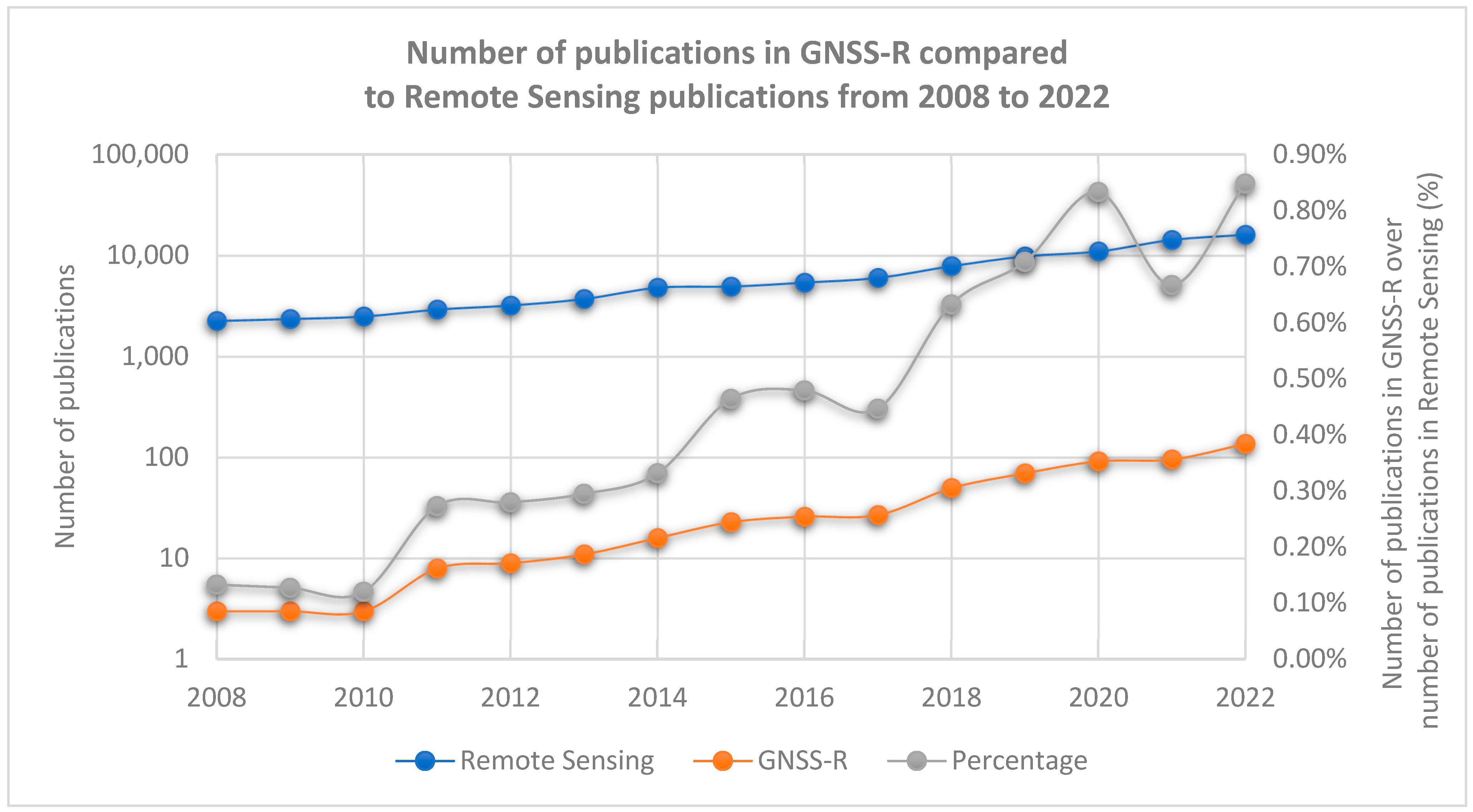
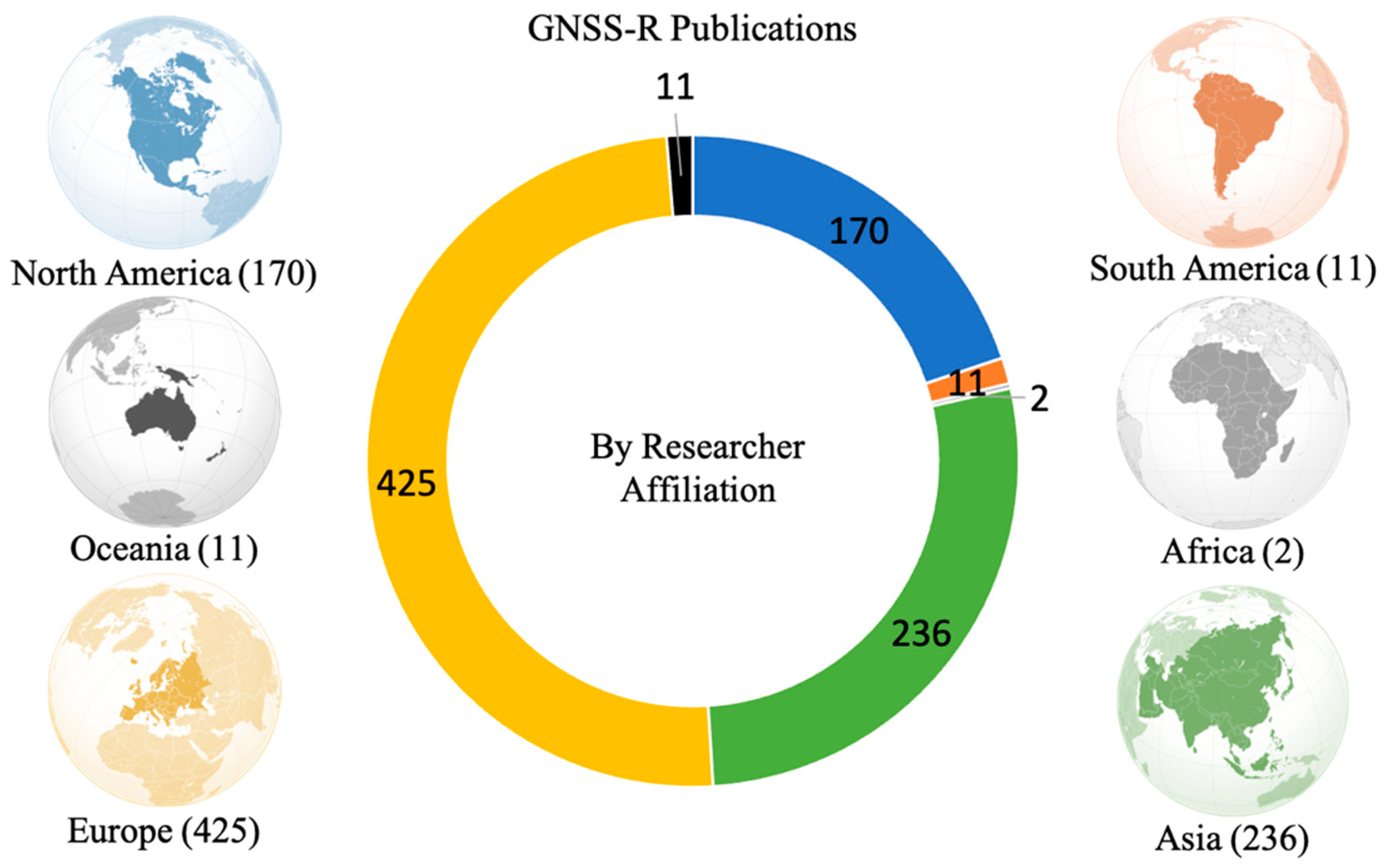
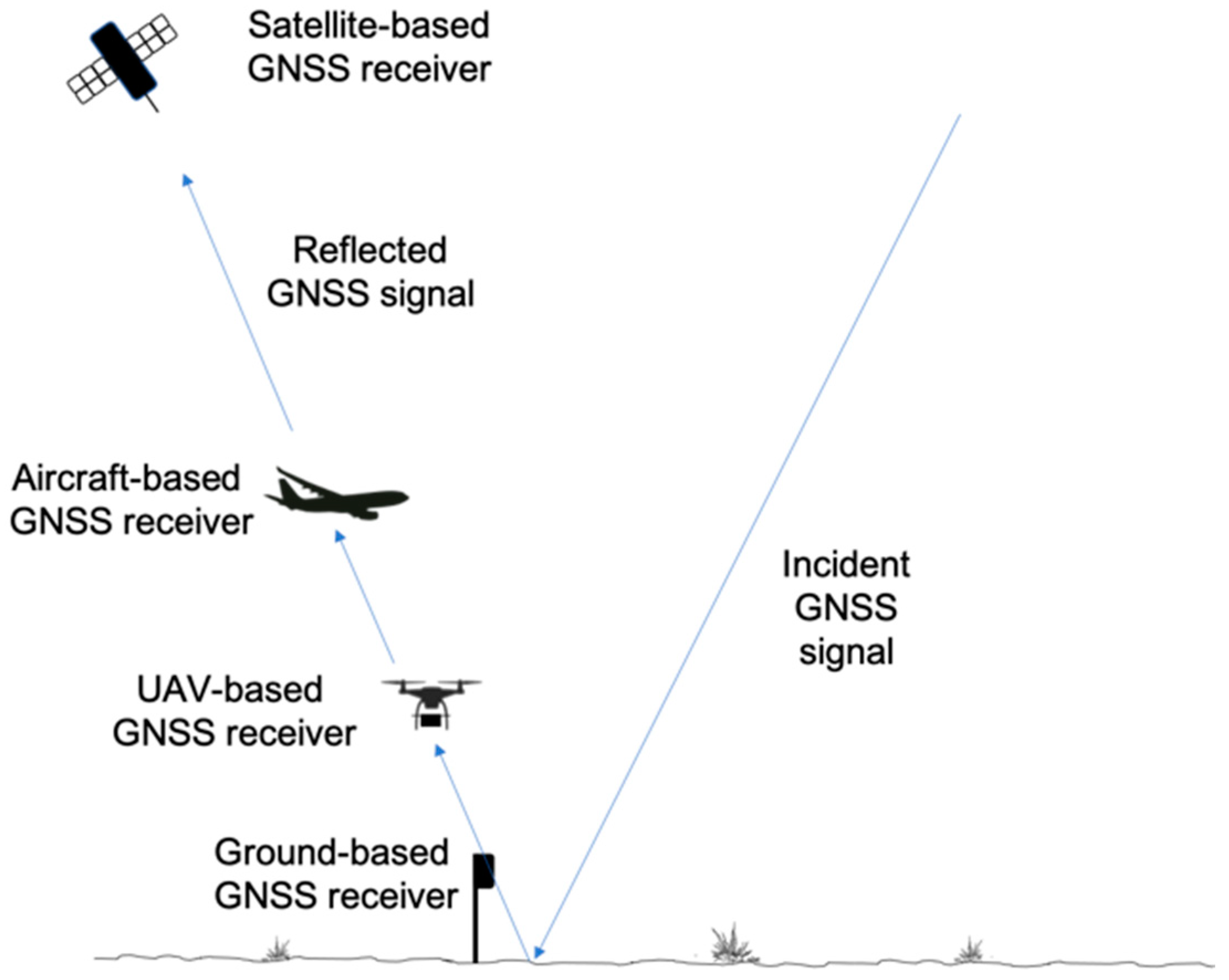
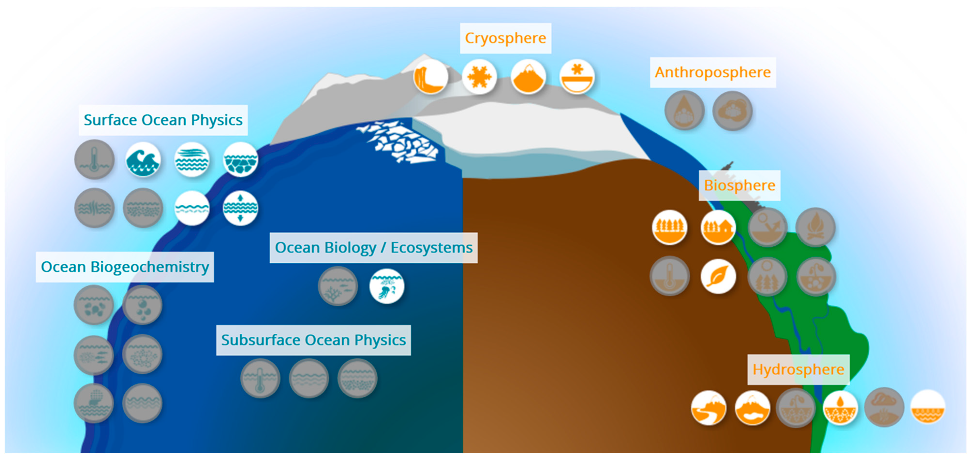
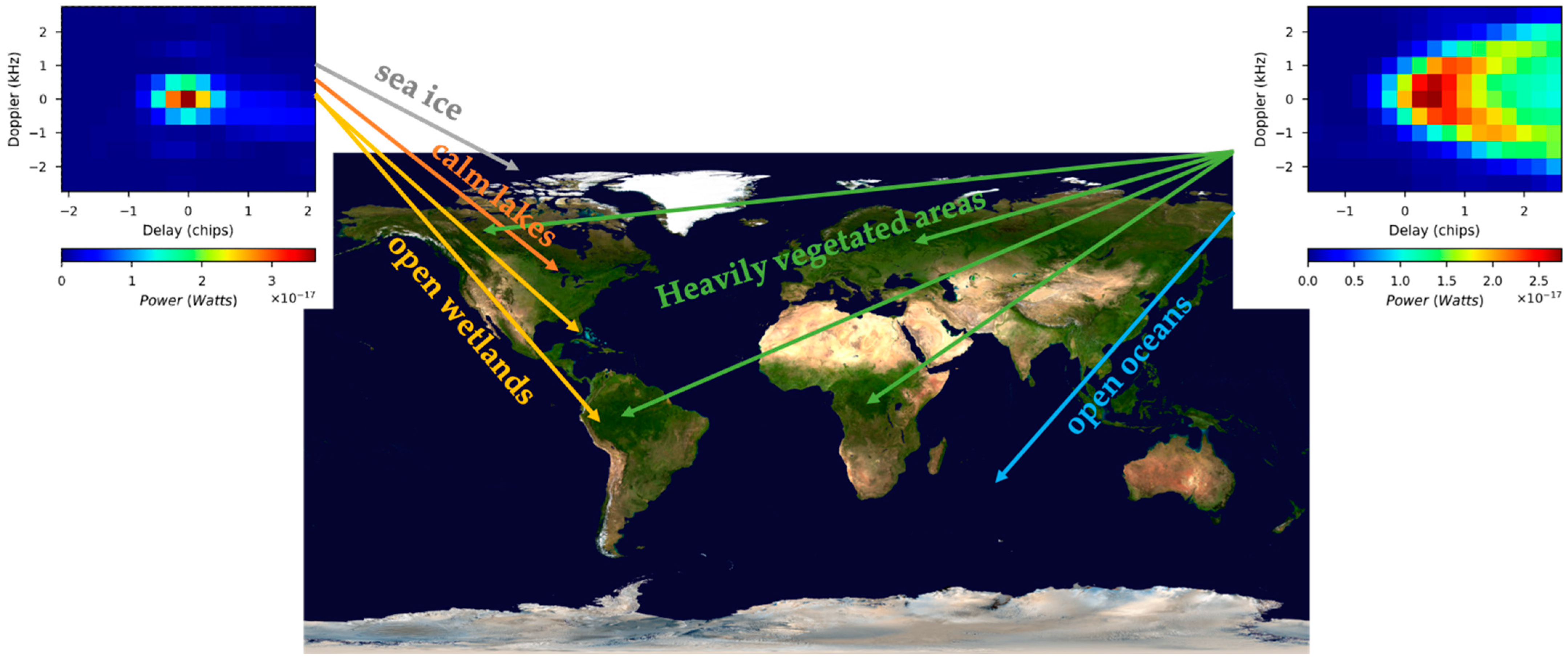


