Satellite-Based Estimation of Soil Moisture Content in Croplands: A Case Study in Golestan Province, North of Iran

Abstract

Soil moisture content (SMC) plays a critical role in soil science via its influences on agriculture, water resources management, and climate conditions. There is broad interest in finding relationships between groundwater recharge, soil characteristics, and plant properties for the quantification of SMC. The objective of this study was to assess the potential of optical satellite imagery for estimating the SMC over cropland areas. For this purpose, we collected 394 soil samples as targets in Gonbad-e Kavus in the Golestan province in the north of Iran, where a variety of crop types are cultivated. As input data, we first computed several spectral indices from Sentinel 2 (S2) and Landsat 8 (L8) images, such as the Normalized Difference Water Index (NDWI), Modified Normalized Difference Water Index (MNDWI), and Normalized Difference Salinity Index (NDSI), and then analyzed their relationships with surveyed SMC using four machine learning regression algorithms: random forests (RFs), XGBoost, extra tree decision (EDT), and support vector machine (SVM). Results revealed a high and rather similar correlation between the spectral indices and measured SMC values for both S2 and L8 data. The EDT regression algorithm yielded the highest accuracy, with an R² = 0.82, MAE = 3.74, and RMSE = 1.08 for S2 and R² = 0.88, RMSE = 2.42, and MAE = 1.08 for L8 images. Results also revealed that MNDWI, NDWI, and NDSI responded most sensitively to SMC estimation.

1. Introduction

The total amount of water on the surface of the land and in the subsurface is known as terrestrial water storage. In addition to groundwater, snow, ice, water trapped in the plants, river, and lake water, it also comprises surface soil moisture and in the root zone [1]. Surface soil moisture is the water that is in the upper 10 cm of soil, whereas root zone soil moisture is the water that is available to plants—generally considered to be in the upper 200 cm of soil. Soil moisture content (SMC) refers to both the surface and root zone, although the surface is more commonly targeted. SMC plays an essential role in agricultural operations, hydrological processes, and the complex cycles of water, energy, and carbon [2,3]. SMC is one of the main factors influencing plant growth and climate conditions by governing temperature and water budgets between the surface and atmosphere [4,5]. SMC is a significant environmental stressor in areas with low soil water contents, poor soil drainage, or high water table fluctuations [6]. SMC also serves as a key indicator of water stress, making it essential for assessing agricultural drought, planting dates, and harvest times [7,8].

Although, SMC is not only a vital component of the Earth’s ecosystem, it also provides a critical relationship between the land surface and the atmosphere [9]. Accurate SMC estimation is essential in hydrological and agricultural applications, since the hydric state of the soil is a primary parameter in the rainfall–runoff process [10]. Soil surface moisture changes rapidly under the influence of environmental conditions such as sunlight, rainfall, and evapotranspiration. Changes in topography also cause the Earth’s surface to alter the SMC [9]. While the estimation of the SMC can be achieved in multiple ways, they can be generalized into two groups: direct and indirect methods [11,12]. In direct methods, the mass of water divided by the mass of the soil is calculated. In indirect methods, the SMC is estimated by sensors and other variables closely related to the SMC [13]. Traditionally, direct methods such as weighting methods, neutron meter radiological methods, and soil–water dielectrics tend to be more reliable and provide more accurate SMC determinations than indirect methods such as tensiometers, gypsum blocks, neutron probes, pressure plates, and the pressure membrane apparatus [14]. The drawback of conventional direct methods is that, despite their simplicity, they are not applicable at large spatial and temporal scales [15]. Instead, indirect measurements of the SMC became common practice in the recent decade.

SMC is one of the fundamental factors of environmental biology that has a range of direct effects on plants, animal life, and microorganisms. Therefore, spatiotemporal awareness is essential in hydrological studies, soil sciences, environment, meteorology, irrigation, and drainage to improve water consumption efficiency [16]. While a range of on-site and laboratory methods can be applied for spatially explicit SMC measurement, each of them has disadvantages and advantages. For instance, laboratory methods are time-consuming, and soil sampling disturbs soil structure and can cover only a limited size of area. Moreover, in situ measurements of the SMC go along with pedoturbation [17]. Optical RS data became an attractive source of information to estimate different soil properties, such as the SMC [18,19]. Alternatively, satellite data can supply near real-time spatial–temporal observations over a vast area, which is hard to achieve using common field measurements [20]. Among the powerful RS techniques for precise estimation of this variable are data-driven models.

Nowadays, machine learning techniques offer flexible regression models for quantifying surface cover properties. They became mainstream algorithms in image processing and have also been successfully applied for estimating the SMC [21]. For instance, a recent study demonstrated that the XGBoost algorithm is significantly more effective than random forest (RF) using Landsat 8 (L8) to estimate the SMC [22]. Machine learning techniques are increasingly widely used for predicting soil moisture using remote sensing data [23,24]. For instance, in a semiarid region of Iran, the SMC was estimated using machine learning algorithms [25]. The results revealed that the RF model outperformed the other models in the validation of soil moisture estimation. Other machine learning algorithms were also evaluated in the context of SMC estimation [26].

According to several studies, RF models predict soil properties much more accurately than other regression techniques [27,28]. However, a systematic evaluation based on the most commonly used satellite images, i.e., Sentinel-2 and Landsat, and four powerful machine learning algorithms in the context of SMC estimation is still missing. Given all this, the objectives of this study were to: (i) investigate the effectiveness of different machine learning models for predicting the SMC in the crop fields in the north of Iran and (ii) identify the key predictor variables affecting SMC prediction using machine learning approaches.

2. Materials and Methods

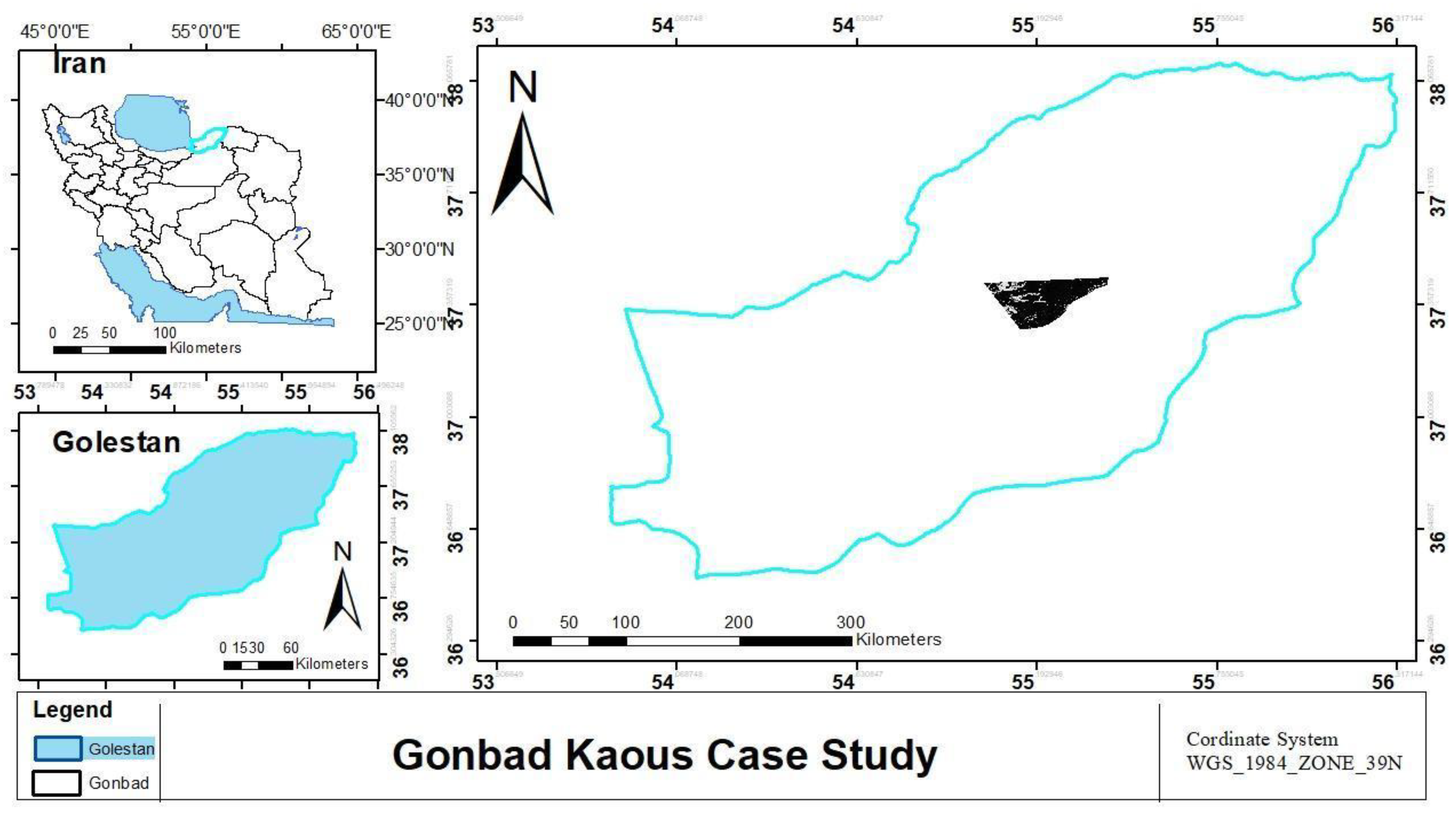
2.1. Study Area

The study area covers approximately 34,330 ha of Gonbad-e Kavus in the Golestan Province in northern Iran and is located between 55°10′ and 55°22′E longitudes and 37°15′ and 37°25′N latitudes (Figure 1). This vast region is divided into two physiographic units: alluvial plains and plains over Gorgan River traces, all with sediments of loess origin covering some Caspian Sea formations after the retreat. According to the Ombrothermic Diagram, the climate of this region is hot, semiarid, or moderate. Most rainfall occurs in the cold season; the summer is hot and dry. The hottest month of the year is August, and the coldest one is February; the average annual rainfall is 461 mm, and the total evapotranspiration potential is 1270 mm per year according to the Penman–Monteith method. Soil types were classified as typical Mollisols based on the USDA Soil Classification System.

Wheat and barley are cultivated in November and harvested in June in this area. Cotton, tomato, or watermelon are planted afterward and harvested before planting wheat and barley. These summer crops need irrigation, but wheat and barley are usually grown rain-fed. Some farmers may irrigate them once or twice in March and April. The pipe drainage system is used in this area for salinity control.

2.2. Field Sampling

In May 2020, 394 surface soil samples (0–10 cm depth) were collected. The following criteria are considered for in-field sampling:

• Predetermined points were identified on the ground by a hand-held GPS receiver. Eight random 10 cm deep core soil samples were obtained from 10 m diameter circles that were centered at the above-mentioned points. Eight samples from each point were mixed and combined into one sample.
• Soil samples were collected near the dates of the S2 and L8 acquisitions
• Fields had sparse crop cover at the time of sampling.

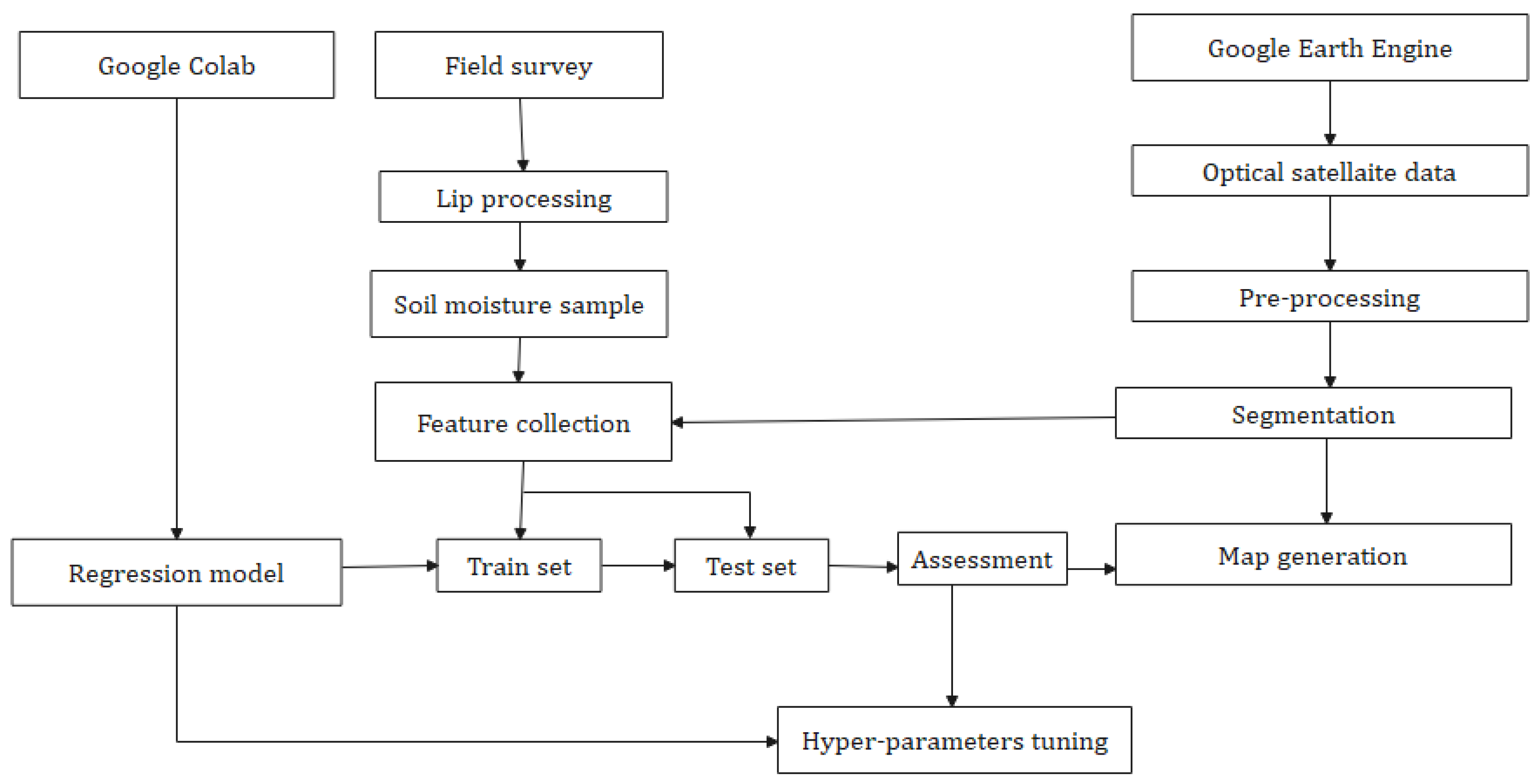
We deployed a direct method for SMC sampling, which is a volumetric SMC determination procedure. The soil samples were collected using the soil sampling ring from a depth of 10 cm, and these soil samples were packed in bags. Soil samples were transported to the laboratory, and soil weight was measured using a digital scale. Subsequently, samples were oven-dried at 105 °C for 24 h [29]. After complete drying of the samples, the difference in weight between the wet and dried samples was calculated, and according to Equations (1)–(3), the volumetric SMC was calculated:

$${\theta }_m=\frac{M_w}{M_s}\times 100$$

(1)

where θ_m is the gravimetric soil moisture, M_w is the weight of wet soil, and M_s is the weight of dry soil. So, the bulk density of the soil, P_b, is defined as:

$$P_b=\frac{M_s}{V_t}$$

(2)

where V_t is the volume of the soil sample ring. Therefore, the volumetric water content, θ_v, is defined as Equation (3):

$${\theta }_v=P_b\times {\theta }_m\times 100$$

(3)

2.3. Methods

One of the prominent aspects of this study is that the SMC mapping is entirely based on free, open-source cloud computing platform resources provided by Google, including the Google Earth Engine (GEE) and Google Collaboratory (COLAB), ensuring full transparency and applicability to other regions. The COLAB programming environment is establishing itself as one of the most popular platforms for scientific computing. Furthermore, preprocessing steps such as simple noniterative clustering (SNIC) segmentation [30] are carried out within the GEE platform. A flowchart illustrating the steps for SMC prediction using satellite data is given in Figure 2. Other processing steps, including the regression analysis, hyperparameter tuning, etc., were realized within COLAB. Regarding the used satellite imagery, the multispectral bands recorded by each of the sensors L8 and S2 are given in

Table 1. Corresponding Landsat 8 (L8) and Sentinel 2 (S2) bands and spatial resolution.

Satellite	Sensor	Bands	Wavelength	Spatial Resolution (m)
L8	Operational Land Imager (OLI)	Band1-Coastal aerosol	0.43–0.45 µm	30
		Band2-Blue	0.45–0.51 µm	30
		Band3-Green	0.53–0.59 µm	30
		Band4-Red	0.64–0.67 µm	30
		Band5-NIR	0.85–0.88 µm	30
		Band6-SWIR 1	1.57–1.65 µm	30
		Band7-SWIR 2	2.11–2.29 µm	30
		Band8-Panchromatic	0.5–0.68 µm	15
		Band9-Cirrus	1.36–1.38 µm	30
		Band10-TIRS1	10.60–11.19 µm	100
		Band11-TIRS2	11.50–12.51 µm	100
S2	Multispectral Imager (MSI)	Band1-Coastal aerosol	443 nm	60
		Band2-Blue	490 nm	10
		Band3-Green	560 nm	10
		Band4-Red	665 nm	10
		Band5-VNIR	705 nm	20
		Band6-VNIR	740 nm	20
		Band7-VNIR	783 nm	20
		Band8-VNIR	842 nm	20
		Band8Aa-VNIR	865 nm	10
		Band9-SWIR	940 nm	20
		Band10-SWIR	1375 nm	60
		Band11-SWIR	1610 nm	20
		Band12-SWIR	2190 nm	20

.

2.4. Preprocessing

Imagery data from the L8 and S2 are used as provided by GEE. The data do not require preprocessing or initial correction (geometric, radiometric, etc.) and are readily available for processing. In GEE, L8 and S2 can be called with any processing level. Atmospheric correction images of the L8 OLI Surface Reflectance Tier 1 and S2-A MSI (L2A) are used. S2 and L8 satellite images were imported over the study site and were clipped with a study area shapefile. Both the images were filtered by date from April to July 2020 and were used as input for SMC estimation through the running of the trained regression models. The imported images were then filtered to mask cloud images. These data have been atmospherically corrected using GEE. Masking clouds and cloud shadows in S2 surface reflectance data using COLAB. The S2 image was filtered for clouds with the metadata CLOUD_PIXEL_PERCENTAGE for a cloud pixel percentage of less than 10%. In the case of L8, the metadata CLOUD_COVER of 5% was applied to mask the clouds. The following satellite bands were selected for the regression analysis: eleven S2 bands (2,3,4,5,6,7,8,8a,9,10,11) and six L8 bands (2,4,3,5,6,7). Widely used indices, such as water-based, vegetation-based, and salinity-based, were derived for analysis in the regression algorithms, as shown in

Table 2. Indices used to L8 and S2 data.

Indices	Formula	References
Salinity index—S1	SI1 = sqrt ($Gree{n}^2$ + $Re{d}^2$)	[31]
Salinity index—S2	SI2 = sqrt (Green × Red)	[32]
Salinity index—S3	SI3 = (Blue × Red)	[33]
Salinity index—S4	SI4 = (Red × NIR)/Green	[34]
Salinity index—S5	SI5 = Blue/Red	[34]
NDSI	NDSI = (Red − NIR)/(Red + NIR)	[33]
NDVI	NDVI = (NIR − Red)/(Red + NIR)	[35]
SAVI (L = 0.5)	SAVI = (1 + L) × (NIR − Red)/(L + NIR + Red)	[36]
Vegetation soil salinity index (VSSI)	VSSI = 2 × Green − 5 × (Red + NIR)	[37]
NDWI	NDWI = (SWIR − NIR)/(SWIR + NIR)	[38]
Extended EVI	2.5 × (NIR + SWIR1-Red)/[NIR + 2.5 × (SWIR1 + 6 × NIR + Red 7.5 × SWIR1 − Red) × Blue + 1	[39]
MNDWI	MNDWI = (−SWIR)/(Green + SWIR)	[40]

.

2.5. Feature Collection: Spectral Indices

The feature extraction was carried out in COLAB based on the data measurements. Then, independent and dependent (i.e., SMC) variables were selected. For the independent variables, 11 spectral indices were selected. In our regression analysis, we evaluated the correlation coefficient between SMC measurements, vegetation indices, and salinity indices. Moreover, the accuracy of the model for SMC estimation was improved using feature-selected methods, which reduce feature set redundancy [17].

2.5.1. Vegetation Index

The normalized difference vegetation index (NDVI) is the most common index used to assess crop greenness directly and crop–water relationships indirectly. The NDVI is calculated by standardizing the difference between the near-infrared (NIR) band and red band (RED) reflectance bands [41]. The normalization results in NDVI ranges between 1 and −1, where negative values indicate a lack of vegetation and positive values a presence of vegetation. The equation is given below:

$$NDVI=\frac{NIR-RED}{RED+NIR}$$

(4)

2.5.2. Soil Indices

Huete [42] introduced the soil-adjusted vegetation index (SAVI) to compensate for bare soil damage. These vegetation indices are used specifically for various applications. This index can minimize the soil brightness correction factor in regions where vegetative cover is low. NIR and Red refer to the bands related to those wavelengths, and an L value equal to 0.5 is recommended in previous reports [42]. SAVI is defined below:

$$\mathrm{SAVI}=\frac{\left(1+ \mathrm{L}\right)\times \left(\mathrm{NIR} - \mathrm{Red}\right)}{\left(\mathrm{L} + \mathrm{NIR} + \mathrm{Red}\right)}$$

(5)

2.5.3. Water Indices

The normalized difference water index delineates open water properties in a satellite image, allowing a water body to stand out against the soil and vegetation. It makes use of the NIR and short-wave infrared (SWIR) reflectance to increase the presence of such features while removing the presence of soil and vegetation properties. Equations are given below:

$$NDWI=\frac{NIR-SWIR}{RED+SWIR}$$

(6)

The modified normalized difference water index (MNDWI) uses green and SWIR bands to enhance open water features. The MNDWI is not only more suitable for enhancing and extracting water, but it also has an advantage in reducing noise over the NDWI. The MNDWI can enhance open water features while effectively repressing and even eliminating land noise as well as vegetation and soil noise [38].

$$MNDWI=\frac{Green-SWIR}{Green+SWIR}$$

(7)

2.5.4. Salinity Indices

NDSI is a measure of the relative magnitude of the reflectance differentiation within visible (green) and SWIR [43]. The salinity index indicates the salt content of soils. One of the most frequent causes of land degradation is soil salinity, particularly in areas where precipitation exceeds evaporation. Low values denote lower salinity, whereas high values denote higher salinity. Several soil salinity indices have been developed [32], and their different types have been described in Table 2.

2.6. Segmentation

Object-oriented segmentation is a beneficial process for high-resolution image processing. The advantage is that the pixels cannot be interpreted alone, and in addition, in the case of high-resolution images, the classification of the pixels leads to decreased noise. Segmentation means a group of neighboring pixels within an area where similarities such as numerical value and texture are the most important standard features. The segmentation of an image can be used to enhance the performance and be less noisy in optical data, object-based analysis, and ground surface investigation. A multiresolution segmentation method was used for extracting a map to show the nature of variations. To achieve a balance between segment indices, spectral and structural specifications of landscapes are considered, because proper indices for segmentation by the multiresolution method are selected by trial and error and segmentation is required to be repeated with different indices and combinations of their different weights. Accuracy in segmentation from the viewpoint of spatial conformations with landscape positions affects final accuracy in imagery classification and identification.

The optimal levels of segmentation were identified given the current data based on the available spectral and spatial resolution, using trial and error at different levels. For this purpose, multiple segmentations were achieved by using S2 and L8 images and also numerical contour maps, slope maps, geological maps, and soil base maps as main layers, their geocoding processing with trial and error, and then producing a combination of effective parameters of different weights on segmentation such as scale, shape, and compactness.

In GEE and in interaction with COLAB, training soil samples were first identified on the segmented images, and different indices with respect to each object (relevant to the training samples) were analyzed for the selection of the best indices. Then, classification was processed using selected indices and predetermined thresholds for each index. Finally, experimental samples were used for the evaluation of the accuracy of each index for classification and the introduction of semiautonomous modeling for evaluating SMC. The parameters and characteristics of mean and standard deviation for S2 bands B3, B8, B12, and L8 bands B3, B5, B7, perimeter, area, NDWI, and NDVI indices, etc., are used to improve the results of the algorithm’s nearest neighbor object-oriented method.

SNIC was used for segmentation. As opposed to other superpixel algorithms, SNIC has the advantages of not only easy calculation, low memory consumption, and high speed, but also without subsequent area connection operations, no multiple iterations, lower pixel accesses, and distance calculations [44]. SNIC is calculated as follows (Equation (8)). Assuming the spatial position is a and the color value is b, the distance formula from the j-th candidate pixel to the k-th superpixel centroid [30]:

$$a_{j,k}=\sqrt{{\left(\frac{d_a}{S}\right)}^2+{\left(\frac{d_b}{m}\right)}^2}$$

(8)

where $d_a$ and $d_b$ are the spatial and color distances between the candidate point and the cluster center, and sequentially the calculation formula is as follows:

$$d_a=\parallel a_j-a_k\parallel$$

(9)

$$d_b=\Vert b_j-b_k\Vert$$

(10)

where a_i and a_k represent the positions of candidate points and cluster centers, b_i and b_k represent their colors, and s and m represent the normalization factors for spatial and color distances. For an image of N pixels and K superpixels, the value of s is p (N/K). The value of m, commonly known as the density factor, is set by the user [30].

2.7. Machine Learning Regression Algorithms

Random forest (RF) [45], XGBoost [46,47], extra tree decision (ETD) [48], and support vector machine (SVR) [49] are among the popular shallow machine learning methods in RS applications. These algorithms are briefly outlined below.

SVR is one of the most prevalent supervised machine learning algorithms. Although SRV is mainly used in classification tasks, it is also appropriate for regression tasks. SVR involves the optimization of two essential parameters of support vector machines, which are C and gamma [49].

RF is a machine learning algorithm with usability and is more accessible than other algorithms that often deliver excellent results even without adjusting their hyperparameters. Due to its simplicity and usability, this algorithm is the most commonly used machine learning algorithm for both classification and regression [45,50]. RF is flexible and easy to use because only a few parameters need to be set by the user.

The XGBoost is a supervised learning algorithm that aims to accurately predict a target variable by compounding an ensemble of estimates from a set of more superficial and weaker models, and has become a powerful algorithm [51]. The influence of the system has been extensively documented in a number of machine learning and data mining challenges [46].

ETD and RF are related regression tree algorithms. RF makes use of bootstrap replicas and subsamples the input data with substitution, while ETD uses samples without replacement of the entire main sample. RF chooses the optimum split versus ETD, which chooses it randomly [48].

2.8. Train and Test Dataset Partitioning

This study splits the dataset into 70% training data and 30% testing data. Then, models are trained and tested on the volumetric SM data. We collected 394 soil samples for model building and validation. In these, 269 samples (70%) were used as calibration data and 125 samples (30%) as validation data.

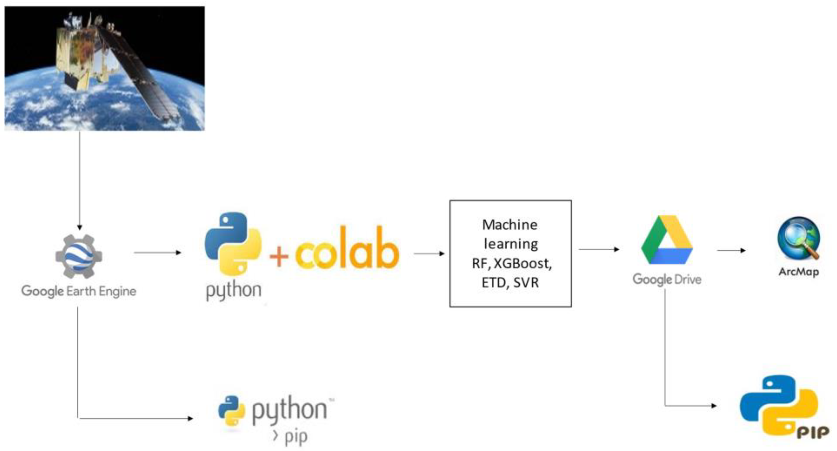
2.9. Implementation Platform

Google Earth Engine (GEE) is a planetary-scale web portal offered by Google. GEE uses Google’s cloud-based computing and approachable, open-access remote sensing datasets. GEE has the ability to provide and process big geodata that eases the scientific discovery process by giving users free access to large remotely sensed datasets [52]. The outstanding feature of this GEE is that it is free. It provides access to the databases of European and American space agencies, as well as other databases. For instance, regarding optical data, both raw radiance products and atmospherically corrected surface reflectance products are provided. At the same time, the Google Colaboratory (Colab) is a free cloud notebook environment that has free access and is automatically saved to Google Drive on graphics processing units (GPUs). The benefit is that COLAB can easily access GEE and supports a diversity of machine learning libraries, which can be quickly loaded into a notebook (Figure 3). Codes for the machine learning algorithms utilized in this paper are accessible at scikit-learn.org.

2.10. Hyperparameters Tuning

Hyperparameter tuning is the process of determining the appropriate set of hyperparameters that optimize the machine learning parameters. Setting the suitable mix of hyperparameters enables to extract the maximum performance models. Hyperparameters are essential in building robust and precise models. Hyperparameter tuning helps find the equilibrium between bias and variance. Therefore, it prevents the model from overfitting or underfitting. Concerning the tuning of the hyperparameters in estimating SMC, it is necessary to understand their role in achieving accurate and robust models. Machine learning has a different adjustment of hyperparameters that govern the learning model [53].

One of the well-known methods for optimizing hyperparameters is grid search. By identifying the best combination of hyperparameter values, it can improve model performance and hence significantly decrease the parameter optimization time [54]. The data was split into 70% training and 30% testing. Grid search and 10-fold or 5-fold cross-validation on the training dataset were used to discover the most suitable regression parameters. The test dataset was used to make an estimate of the performance of the chosen model.

The RF algorithm has a few hyperparameters to tune [55]. The 10-fold cross-validation method was used in conjunction with a grid search to improve model performance.

Table 3. Grid search hyperparameters for RF.

Parameters	Range	Optimum Value
n_estimators	70 to 150	100
Max feature	(Auto, SQRT, Log2)	log2
Max depth	1 to 10	3
min_samples_spli	(2, 4, 8)	2
bootstrap	(True, False)	False

shows the RF hyperparameter ranges and the optimized values identified by the grid search.

To determine the suitable kernel function and the C parameter for the SVR algorithm, grid search was used, and the gamma parameter was set to its default value. Hyperparameters, with the great results acquired with regression c = 15, gamma = scaler, and kernel = RBF, have been tested (

Table 4. SVR grid search parameters.

Parameters	Range	Optimum Value
C	(1, 5, 10, 15, 20, 25, 35, 40)	15
Gamma	(scale, auto)	scaler
Kernel	(linear, poly, rbf, sigmoid)	rbf

).

Regarding XGBoost, similar to RF, the algorithm is tuned using multiple hyperparameters. A grid search on hyperparameters with 10-fold cross-validation was implemented to discover the great model according to R² metrics (

Table 5. The grid search XGBoost regression modeling hyperparameters.

Parameters	Range	Optimum Value
n_estimators	70 to 500	200
Max depth	1 to 10	8
gamma	0.1–1	0.1
min_child_weight	3 to 10	5

).

The grid search from ETD regression modeling hyperparameters is shown in

Table 6. ETD regression modeling hyperparameters from the grid search.

Parameters	Range	Optimum Value
n_estimators	150	300
Max feature	(Auto, Sqrt, Log2)	auto
Max depth	1 to 10	5
min_samples_split	(2, 4, 8)	2
bootstrap	(True, False)	False

. Hyperparameters, with the best optimum value obtained with regression max feature = auto, n_estimator = 300, max depth = 5, min_samples_split = 2, and without bootstrap, have been tested (Table 6).

The parameters used for segmentation in this research are size = 3, compactness = 5, connectivity = 8, neighborhood = 25. [56] reported that object-oriented classification of image parameters, such as image type, segmentation scale, accuracy assessment type, selected algorithms in classification, educational places, input data, and target classes, are important (

Table 7. Determination of optimum segmentation parameter values for study area.

Argument	Type	Details
Image	Image	The input image for clustering.
Size	Integer, default: 3	The distance between superpixel seeds, measured in pixels. No grid is created if a ‘seeds’ image is provided.
Compactness	Float, default: 5	Compactness factor. Clusters get increasingly compact as values increase (square). Spatial distance weighting is disabled when this is set to 0.
Connectivity	Integer, default: 8	Connectivity. Either 4 or 8.
Neighborhood size	Integer, default: 25	Size of the tile neighborhood (to avoid tile boundary artifacts). Defaults to 2× size.
Seeds	Image, default: null	Any nonzero-valued pixels are used as seed locations if they are present. As determined by “connectivity,” pixels that touch are regarded as belonging to the same cluster.

).

2.11. Accuracy Assessments

Evaluation of the efficiency machine learning models goodness-of-fit metrics, including the coefficient of determination (R²), mean absolute error (MAE), root mean square error (RMSE), and Nash–Sutcliffe model efficiency coefficient (NSE), Akaike information criterion (AIC), and Bayesian information criterion (BIC), were used and calculated according to the following equations:

$$R^2=1-\frac{{\displaystyle {{\displaystyle \sum }}_{i=1}^n}{\left(Q_i-p_i\right)}^2}{{\displaystyle {{\displaystyle \sum }}_{i=1}^n}{\left(Q-\stackrel{-}{Q}\right)}^2}$$

(11)

$$\mathrm{RMSE}=\sqrt{\frac{1}{n}{\displaystyle {{\displaystyle \sum }}_{i=1}^n}{\left(Q_i-p_i\right)}^2}$$

(12)

$$\mathrm{MAE}=\frac{1}{n}{\displaystyle {{\displaystyle \sum }}_{i=1}^n}|Q_i-p_i|$$

(13)

AIC = 2 k − 2 ln(L)

(14)

$$\mathrm{BIC}=\mathrm{kln}\left(n\right)-2\ln \left(\mathrm{L}\right)$$

(15)

$$NS=1-\frac{{\displaystyle {{\displaystyle \sum }}_{i=1}^n}{\left(Q_i-P_i\right)}^2}{{\displaystyle {{\displaystyle \sum }}_{i=1}^n}{\left(Q_i-P_i\right)}^2}$$

(16)

where Q_i is the measured value, P_i is that evaluated by the spatial estimation method, and O and M are the averages of the measured and evaluated SMC. Here, n indicates the number of data points.

The RMSE and MAE values should be closer to zero for optimal prediction, and the R² and NASH-Sutcliffe efficiency values should approach one. The NSE in theory differs in the range −∞ to 1, and higher values of the NSE illustrate well the agreement between predicted values and observations.

2.12. Uncertainty

In this study, k-fold cross-validation was employed to reduce the degree of uncertainty in the modeling outputs. In the k-fold cross-validation, in our case k = 5, the training data were randomly divided into five equal-sized subsets, of which all but one were used for training the predictive model. The procedure is repeated five times and the evaluation criteria are averaged to obtain the final performance.

3. Results

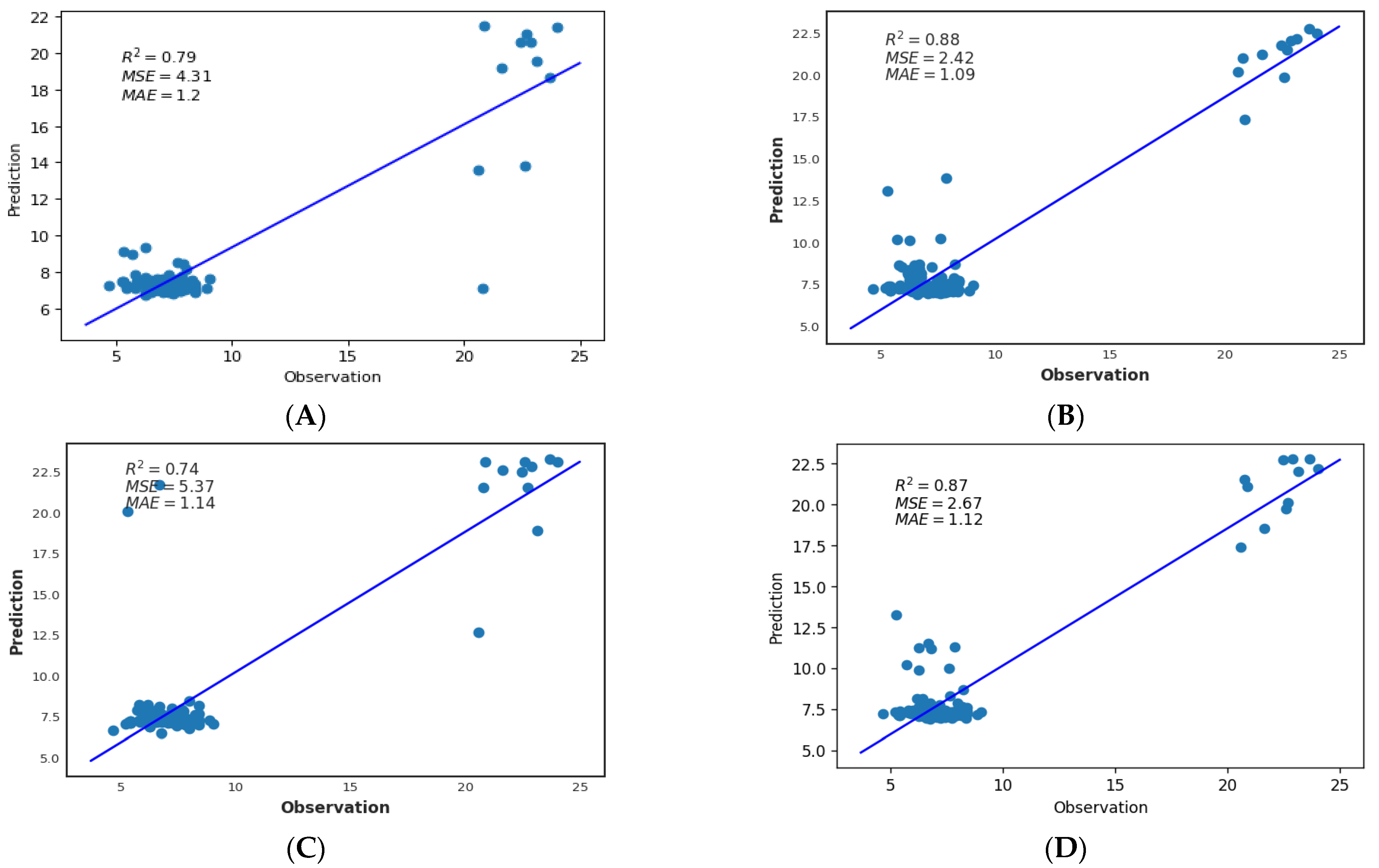
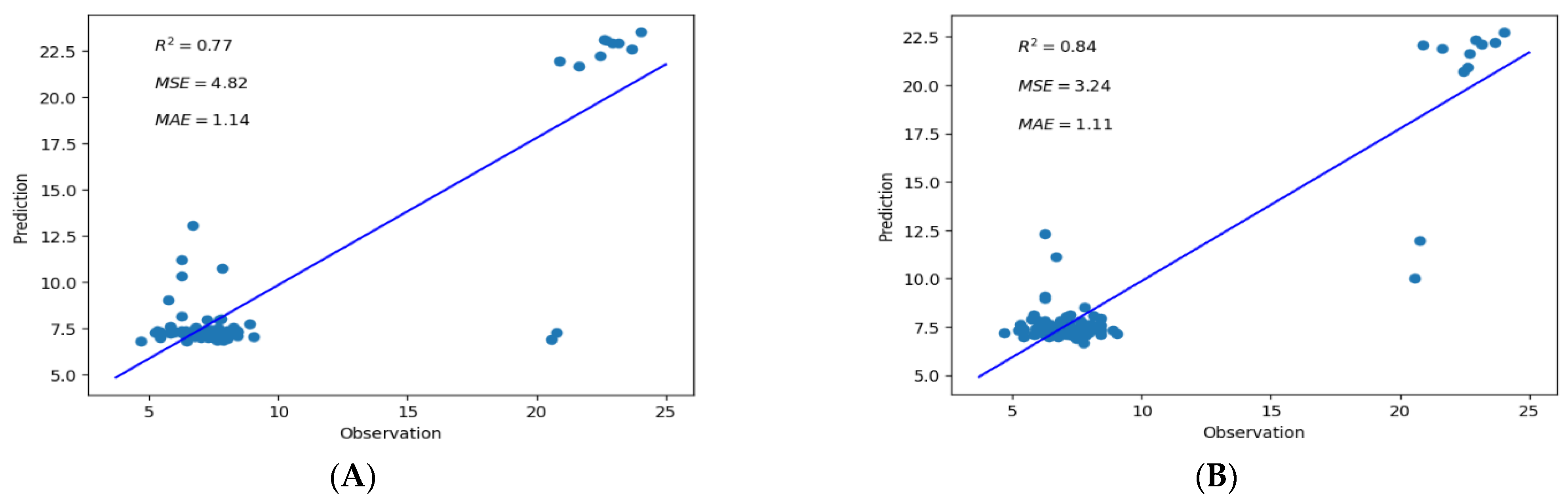
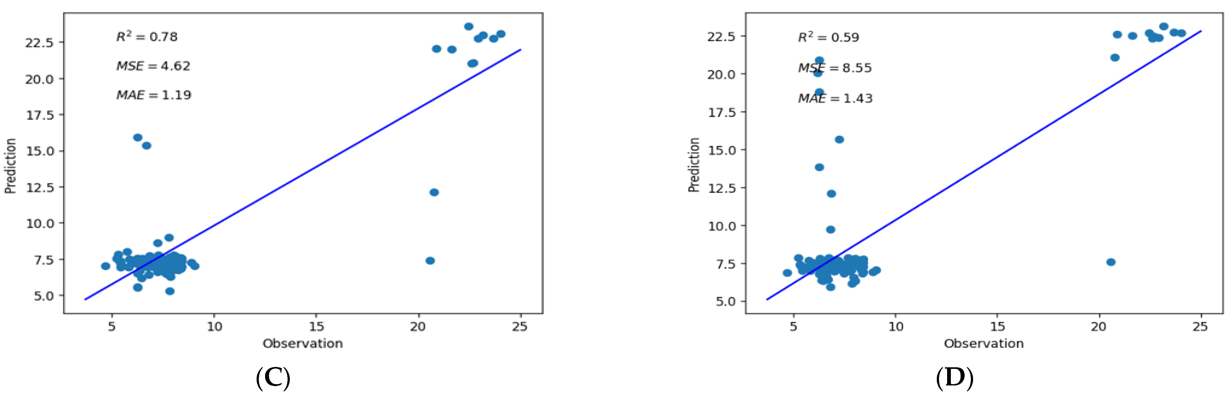
3.1. Model Performance with L8 and S2

As shown in

Table 8. Four machine learning methods (RF, XGBoost, ETD, and SVM) used without segmentation to predict SMC. Best validation results are bolded.

Machine Learning Methods	Landsat 8
	Dataset	R2	RMSE	MEA	AIC	BIC	NSH
	Calibration	0.88	1.58	0.85	136	154	0.88
RF	Validation	0.67	6.64	1.28	233	247	0.67
XGBoost	calibration	0.78	3.13	1.25	323	341	0.78
	Validation	0.64	7.38	1.61	255	283	0.64
ETD	calibration	0.75	5.17	1.22	478	506	0.63
	Validation	0.63	5.57	1.41	222	252	0.75
SVR	calibration	0.59	5.82	1.16	494	516	0.59
	Validation	0.74	5.35	1.42	209	226	0.74
	Sentinel 2
RF	calibration	0.86	1.90	0.86	186	204	0.86
	Validation	0.76	4.76	1.14	194	208	0.76
XGBoost	Calibration	0.93	0.89	0.73	−3	43	0.93
	Validation	0.79	4.24	1.08	196	232	0.80
ETD	calibration	0.90	1.40	0.68	120	166	0.90
	Validation	0.84	3.24	1.11	164	200	0.84
SVR	calibration	0.64	5.11	1.12	457	475	0.64
	Validation	0.83	3.40	1.19	154	168	0.83

, four machine learning models for predicting the SMC without segmentation perform well in terms of evaluation metrics. In these statistical results, we presented the results of the RF, XGBoost, ETD, and SVR models for four input combinations in two datasets, L8 and S2. These results are briefly addressed below.

L8: SMC estimation using L8 data with and without segmentation revealed a slight difference. SVR with an R² of 0.74, MAE of 1.42, and RMSE of 5.35 and ETD with an R² of 0.75, MAE of 1.41, and RMSE of 5.57 have the best model performances, whereas SMC was poorly estimated by the XGBoost model. The EDT outperformed all other models and was therefore selected as the best predictor of the SMC.

S2: In the absence of segmentation, all the machine learning algorithms were tested and found to be capable of predicting the SMC from the S2 data with high accuracy. The ETD and SVM algorithms, although they had a bit better R² with an MAE of lower than 5% SMC performance, have also been the most common algorithms to predict the SMC volumetric cause to solve the nonlinear relation between input and output with a good degree of precision. In this method, XGBoost yielded competitive results (RMSE = 4.24, RME = 1.08, R² = 0.93–0.79). RF models had better performance with these values (RMSE = 4.76, RME = 1.14, R² = 0.76–0.86).

Subsequently, we address the L8 and S2 goodness-of-fit results of four machine learning models for predicting SMC with segmentation in

Table 9. Four machine learning methods (RF, XGBoost, extra tree decision, and SVM) used for segmentation to predict SMC. Best validation results are bolded.

Machine Learning Methods	Regression	Landsat8
		R2	RMSE	MEA	AIC	BIC	NSH
RF	Calibration	0.91	1.27	0.80	82.18	111.09	0.91
	Validation	0.87	2.66	1.11	131.67	153.84	0.87
XGBoost	calibration	0.90	1.41	0.77	105.15	123.21	0.90
	Validation	0.74	5.36	1.13	208.32	222.17	0.74
ETD	Calibration	0.97	0.42	0.50	−224.23	−206.16	0.97
	Validation	0.88	2.42	1.08	114.52	128.37	0.88
SVR	Calibration	0.68	4.53	1.06	435	475	0.68
	Validation	0.78	4.39	1.37	196	227	0.78
	Regression	Sentinel 2
RF	Calibration	0.91	1.28	0.78	87	120	0.91
	Validation	0.79	4.30	1.19	190	215	0.79
XGBoost	Calibration	0.92	1.01	0.71	21	50	0.71
	Validation	0.59	8.55	1.43	294	316	0.59
ETD	Calibration	0.97	0.34	0.45	−245	−274	0.97
	Validation	0.84	3.24	1.11	171	194	0.84
SVR	Calibration	0.83	2.41	0.69	261	297	0.83
	Validation	0.78	4.60	1.32	200	227	0.77

.

L8: The tested machine learning algorithms were capable of predicting the SMC with high precision. The highest R² and NS throughout the training phase were for RF and ETD, whereas XGBoost and SVR performed alike. The good performance had RMAE values of fewer than 5% for all algorithms. The ETD model outperformed the other models based on its lowest RMSE value of 2.42 and higher R² value of 0.97. So, the ETD was evaluated as the best method to predict volumetric SMC. After the ETD model, RF, SVR, and XGBoost performed well based on the RMSE (2.66, 4.39, and 5.36), MAE (1.11, 1.78, and 1.13), and R² (0.87, 0.78, and 0.74) values, respectively. Both ETD and RF models, however, yielded good performances for predicting volumetric SMC.

S2: Based on the evaluation of the results shown in Table 9, it can be observed that the ETD consistently outperformed all other models in estimating SMC, not only for L8 (RMSE = 2.42, RME = 1.08, R² = 0.97–0.88), but also for S2 (RMSE = 3.24, RME = 1.11, R² = 0.97–0.84). The RF (RMSE = 4.62, MAE 1.19, R² = 0.78–0.91) ended up the second-best model for estimating SMC. The XGBoost model (RMSE = 8.55, MAE =1.43, R² = 0.92–0.59) estimated that the SMC had a lower R² than during the validation. In contrast, model SVR (RMSE = 4.82, MAE =1.14, R² = 0.77–0.83) was more than the XGBoost model for estimated SMC in S2. The numerical value shows that the performed ETD regression can control the SMC data by estimating a valuable fitness standard. Based on the results, SMC was predicted with medium accuracy for the ETD (R² = 0.88), whereas the XGBoost led to the poorest estimation accuracy. The SVR had a significant amount of R², while the L8 had a smaller value.

Altogether, Table 8 and Table 9 reveal that the predicted SMC values differed significantly between the model type and the input combinations. As shown in Table 8, XGBoost had a higher R² in L8, whereas it had a smaller R² in S2. Models are contrasted according to the AIC and BIC measures. The Akaike information criterion (AIC) is a measure of the comparative quality of statistical models for a given collection of data. The AIC evaluates the well-being of each model relative to each of the other models. Thus, the AIC provides a means for model choice. BIC is a criterion for model choice among a limited number of models, and the model with the lowest BIC is selected. It is based on the probability function, which is similarly associated with the AIC. The EDT model indicates the most negligible compounds of the AIC and BIC. Therefore, it is evaluated as the most suitable model for L8 and S2.

The 1:1 scatterplots of the actual vs. predicted SMC using the four ML algorithms with two satellite are shown in Figure 4 and Figure 5. It could be seen that each four models (RF, ETD, XGBoost-SVR) had satisfactory goodness-of-fit to the training set. The highest fit was found for the ETD model followed by the RF model. The XGBoost model had a low fit to the test set.

3.2. Uncertainty Analysis of Prediction Soil Moisture Based on Machine Learning

In predicting soil properties, uncertainty is an important concern. There are two primary types of uncertainty in this study: the first is the uncertainty of the model parameters and the second is the uncertainty of the technology used to acquire the satellite data.

In

Table 10. Uncertainty with k-fold cross-validation.

Machine Learning Methods	Regression	Landsat 8
		${\mathbf{R}}^2 (\mathbf{mean} \mathbf{\pm } \mathit{s}\mathit{t}\mathit{d})$	RMSE	MEA
RF	Calibration	0.79 ± 0.09	1.67 ± 0.24	2.84 ± 0.79
	Validation	0.64 ± 0.24	1.87 ± 1.13	2.27 ± 1.28
XGBoost	calibration	0.69 ± 0.45	1.98 ± 0.20	3.24 ± 0.1
	Validation	0.58 ± 22	2.91 ± 1.16	2.41 ± 3.04
ETD	Calibration	0.77 ± 0.49	1.98 ± 1.26	0.50 ± 1.54
	Validation	0.62 ± 0.87	2.42 ± 1.12	1.08 ± 2.86
SVR	Calibration	0.68 ± 1.02	2.64 ± 0.69	2.63 ± 1.37
	Validation	0.56 ± 1.64	3.39 ± 1.39	3.16 ± 1.96
Sentinel 2
RF	Calibration	0.82 ± 0.10	3.18 ± 0.53	1.77 ± 0.15
	Validation	0.76 ± 0.89	2.26 ± 1.02	2.79 ± 1.42
XGBoost	Calibration	0.74 ± 0.14	3.11 ± 0.55	1.75 ± 0.18
	Validation	0.60 ± $0.91$	2.65 ± 1.16	2.68 ± 1.31
ETD	Calibration	0.77 ± $0.15$	1.68 ± 0.16	2.78 ± 0.58
	Validation	0.60 ± $0.29$	2.75 ± 0.91	3.06 ± 2.32
SVR	Calibration	0.73 ± 1.26	3.05 ± 1.62	2.86 ± $1.15$
	Validation	0.58 ± 1.34	4.26 ± 1.54	3.98 ± 1.86

, the uncertainty results for four models are presented, and the results of both Landsat 8 and Sentinel 2 random forest satellites, compared to support vector machine regression, XGBoost, and EDT, have better efficiency in determining uncertainty. Soil moisture nose in the study area. The better performance of RF can be attributed to its ability to model large databases and scale many inputs without change. After the random forest model, the EDT had a better performance for soil moisture, and the support vector machine also had a good performance for uncertainty, while the XGBoost had the lowest performance with mutual evaluation uncertainty of all the algorithms, with a value R² closer to 1, indicating that it has less uncertainty. Although Landsat 8 and Sentinel 2 satellite data are geometrically and atmospherically corrected, they are affected by ground and shadow conditions.

We did not use land attributes in our investigation, which may also lead to potential uncertainties. It is recommended that land attributes be used in future studies to diminish the uncertainty in soil moisture estimation.

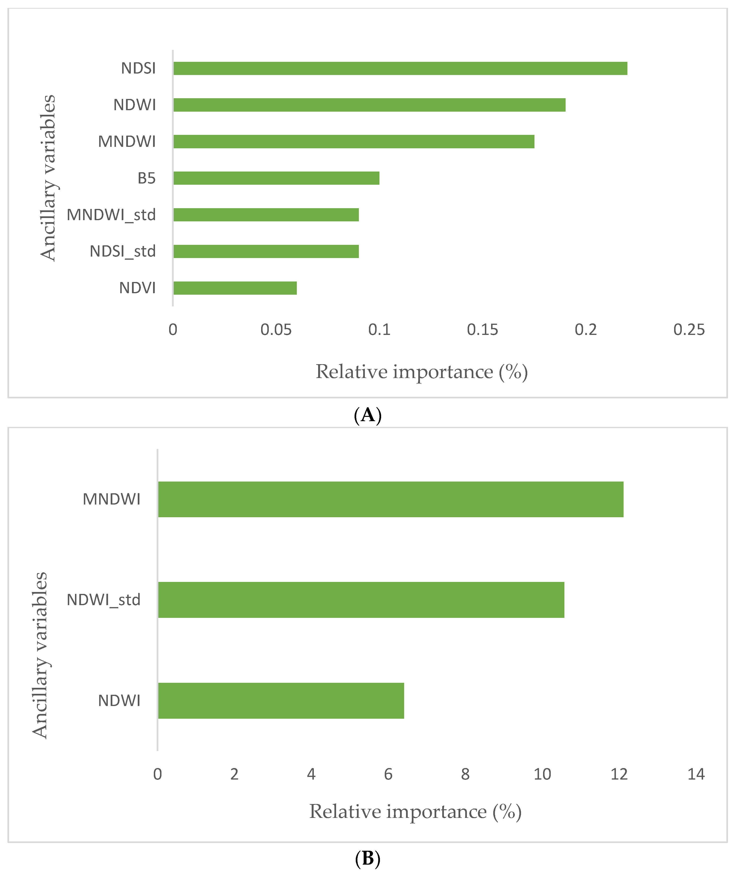
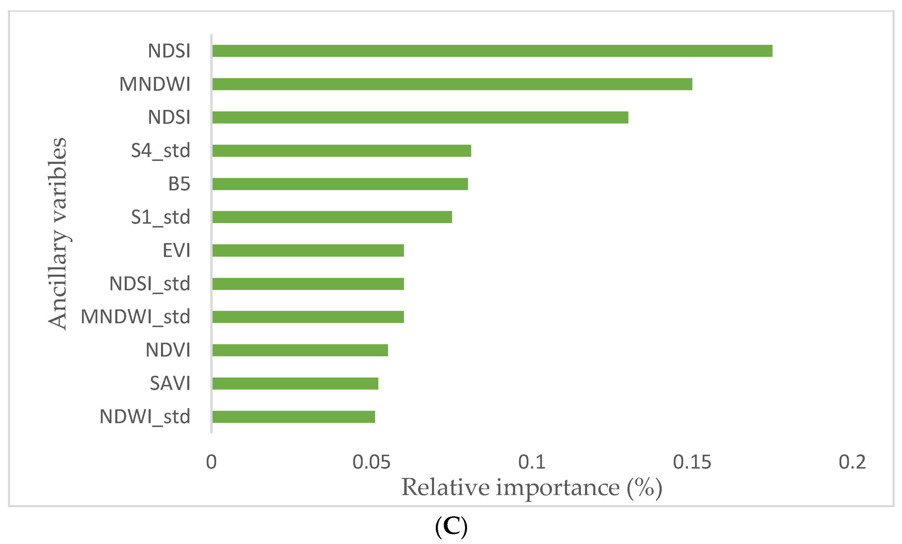
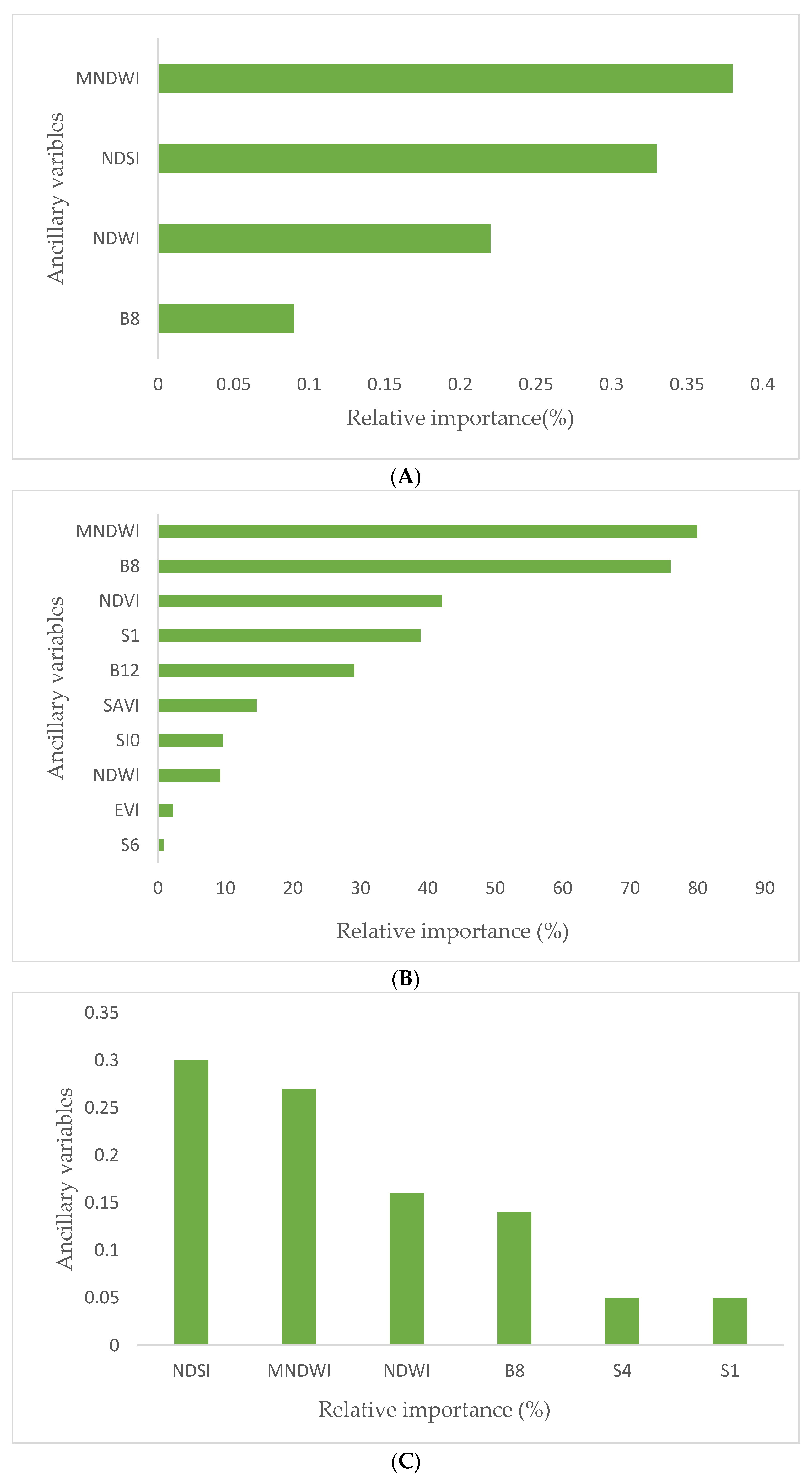
3.3. Feature Importance with L8 and S2

We evaluated the performance of 12 indices and 6 bands as auxiliary features in the models. These selected features not only contribute to the modeling, but also expand the complexity of the model. The ETD, RF, and XGBoost possess the benefit of being capable of grading a predictor variable’s relative significance. As such, we implemented a feature importance evaluation to identify and remove useless features. The feature importance bar graph plot according to these algorithms is displayed in Figure 6A–C. The features are sorted based on their importance. The models measure variable importance based on the percent increase in RMSE and decrease in the p-value.

According to Figure 6A, the NDSI with RF had the highest importance score (0.20), followed by NDWI (0.17), MNDWI (0.16), B5 (0.12), NDWI-STD (0.8), NDSI-STD (0.10), and MNDWI-STD (0.10). In the XGBoost regression, the most important feature was related to the MNDWI index (Figure 6B). According to Figure 6C, with the ETD, the NDSI (0.17) index had the highest importance score. The relative importance of the other indices was as follows: MNDWI (0.16), NDWI (0.11), MNDWI_std (0.07), NDSI_std (0.06), B5 (0.08), S4-std (0.08), S1-std (0.08), NDVI (0.06), SAVI (0.06), EVI (0.06), and NDWI_std (0.04). The L8 dataset was the most important.

In Figure 6, the independent variables with higher RMSE values are illustrated as being more important in predicting the SMC. It was found that soil moisture volumetric prediction relies heavily on water indices in three models (RF, XGBoost, and ETD). Our study also revealed that variables for salinity (S1, S2, S3, S4, S5) expressed lower importance to predict the SMC with machine learning algorithms. The coefficient only works for a linear kernel, while for the RBF, the data space is no longer limited (or, at least, it changes). The NIR and SWIR bands were found to be the most essential of all reflectance bands.

The feature importance score for the S2 data is shown in Figure 7. The several spectral indices we tested were found to be necessary. The low importance of red contrast to the NIR band in evaluating SMC is surprising given the higher sensitivity of the NIR band.

According to Figure 7A, The RF model for prediction of SMC identified the most important covariates as: MNDWI (38%), NDSI (32%), NDWI (22%), B8 (10%).

Results in Figure 7B show that the feature importance, with the XGBoost being most important, was most related to the MNDWI indices B8 and NDVI.

The NDSI (0.30) indices had the highest importance score, and MNDWI was more important with a score of 0.26; there was no difference between B8 and NDVI with similar scores, and S1 and S4 were significant (Figure 7C). Reflectance in the NIR band was the most essential of all the reflectance bands in S2. It can be observed that MNDWI, NDSI, and NDWI indices impact the prediction of the SMC by both the S2 and L8 datasets.

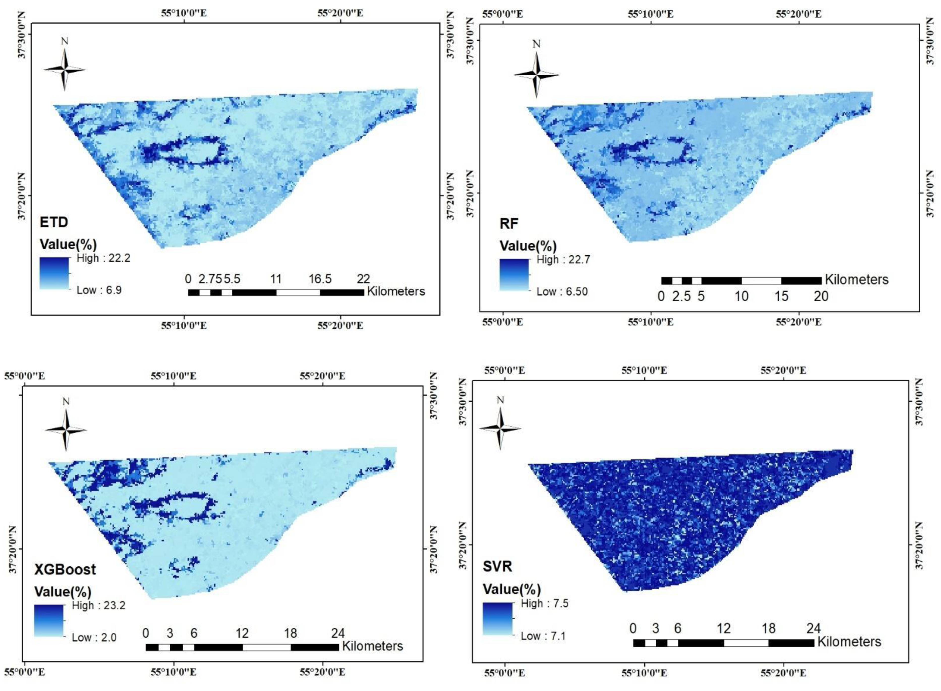
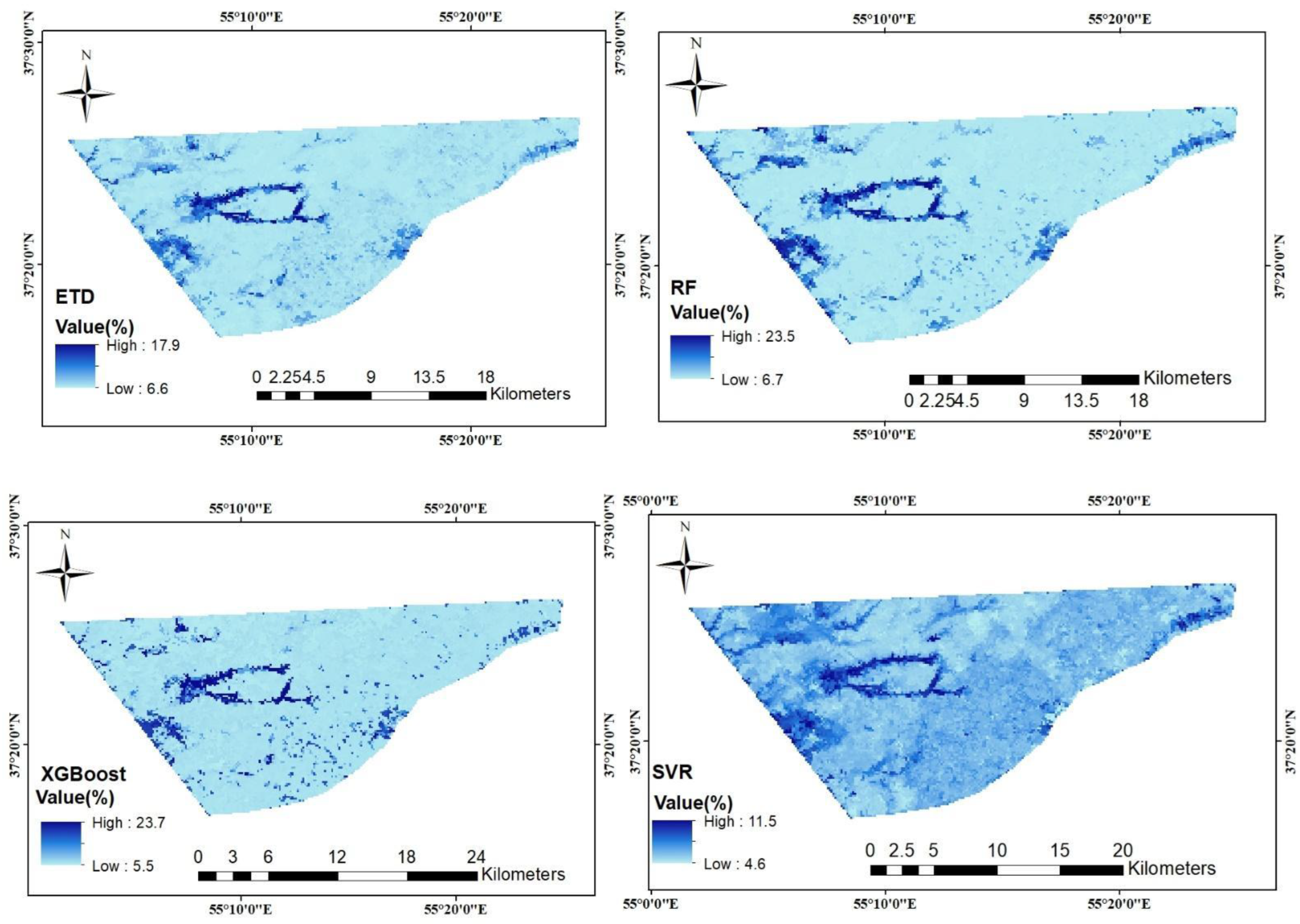
3.4. Generating SMC Map from L8 and S2 Images

The mandatory processing steps of satellite images and field and laboratory work were employed to obtain the SMC. Based on the obtained results, among the sixteen predictor variables of the first and second groups, bands L8 and S2 (B3, B5, B8, B7, and B12) involved in the validation, nine variables, NDWI, MNDWI, NDVI, NDSI, EVI, SI, SAVI, Band 8, and Band 3 changes in humidity variables, are responsive. After confirming the absence of outliers, the normality and correlation of the data were determined, and then the most appropriate effective variables were determined. In the next stage, moisture indices (NDWI and MNDWI), the vegetation index, salinity index, and B3, B8, and B12 were selected to create the final SMC maps. This index has the strongest correlation with the SMC. In Google COLAB, we pip install packages needed for making maps. After the calling and segmentation of images in the COLAB environment, the SMC map was estimated with four machine learning algorithms and applied to L8 and S2 imagery (Figure 8 and Figure 9).

In the region, the parts that were drained had more moisture than the areas that were not drained; moreover, the highest SMC was observed in the drainage outlet areas, which may be due to the relatively low water level while the agricultural lands had a low SMC. In each figure, the four SMC maps are based on the four machine learning algorithms. The RF algorithm is the best algorithm for the surface SMC map. The RF algorithm appeared to be the most suitable algorithm for the surface soil moisture map. Additionally, the decision tree also estimated the better accuracy of the SMC map, which is supported by the SVR model for partial moisture changes. There was a lot of soil moisture at the outlet drainage, which is shown in light blue. It should be kept in mind that the SMC not only increases the amount of absorption by water molecules but also darkens the color of the soil and reduces the reflection from the soil when it gets wet, and usually wet soil is darker than dry soil (in the visible spectrum) because its spectral reflectance decreases. The cause of this darkness is considered to be the water film around the soil particles and its effects. In the drained areas, the soil moisture range was between 10 and 12%; in the nondrained areas, it was between 6 and 10%; in the downstream part, which is near the forest area, the soil moisture was between 10 and 12%. In general, the SMC is variable parameter, and weather conditions, soil texture, and type of crop have an effect on the estimation.

Additionally, the decision tree also estimated the better accuracy of the moisture map, which is supported by the vector machine algorithm for partial moisture changes. There was greater SMC at the outlet drainage, which is shown in light blue. It should be kept in mind that soil moisture not only increases the amount of absorption by water molecules but also darkens the color of the soil and reduces the reflection from the soil when it gets wet, and usually wet soil is darker than dry soil (in the range of the visible spectrum) because its spectral reflectance decreases and the cause of this darkness is considered to be the water film around the soil particles and its effects. In the drained areas, the SMC range was between 10 and 12%; in the nondrained areas, it was between 6 and 10%; in the downstream part, which is near the forest area, the soil moisture was between 10 and 12%. In general, the SMC is a variable parameter, and weather conditions, soil texture, and type of crop have an effect on the estimation.

3.5. Discussion

This research used the machine learning algorithms RF, SVR, ETD, and XGBoost to determine the importance of predictors and predict SMC content and reached the best performance in terms of model accuracy and spatial patterns. Our results revealed a close agreement between the RF and ETD models in estimating SMC. Earlier studies showed that RF models were acceptable compared to those from other models for testing datasets. So, RF was selected as a promising method to predict SMC [25]. The relatively good performance of EDT and RF models is in agreement with earlier studies that found decision-tree-based regression models outperformed other machine learning algorithms, particularly in terrain and soil spatial predictions [21,57]. A previous study demonstrated that due to the hydraulic behavior of water in unsaturated sand, a decrease in spectral reflectance occurs [58]. Soil reflectance correlates nonlinearly with SMC, which correlates well with a curved exponential model between 1100 and 2500 nm [16]. Even though green and red wavelengths have a nonlinear relationship with SMC, the Pearson correlation coefficient represents a fairly weak negative relationship between visible wavelengths and SMC. Several authors earlier studied relationship between optical remote sensing data and SMC with statistical analysis [25,31,59]. The studies reported that the RF process supplied the highest Nash–Sutcliffe efficiency value (0.73) for SMC retrieval covered by the various land-use types. Therefore, RF has been chosen as an excellent method to predict soil moisture [25]. Ref. [50] stated that RF is flexible and easy to use because only a few parameters need to be set by the user. The amount of surface soil moisture was evaluated using remote sensing data. Similarly, the results as reported in [60] showed that machine learning models such as RF, extended trees and SVR perform superior than neural network models, multiple linear regression and classification and regression trees. (CART). This issue is probably due to the optimization algorithms for the selected parameters having different accuracy for training the models. The superiority of RF and SVR over other models has also been reported in various studies [61,62]. In the results presented by [20], two developed tree algorithms and a RFt with a MAE value less than 4% of soil moisture had better performance, which is consistent with other studies, and underlines that regression models based on decision trees work better than other machine learning algorithms. Encouraging results were obtained for the possibility of estimating soil moisture with the research method. Indices (MNDWI, NDWI, NDVI, BT, and LST) were calculated with the help of a combination of two series of telemetry data, including SMOS microwave data and short infrared and near infrared data from the MODIS sensor, to estimate soil surface moisture in the region. The result of this study led to an acceptable relationship between SMC and remote sensing data [63]. The results of that research also indicate the effect of NDWI on the estimation of humidity from satellite data, which is comparable with the results of the research [63]. The results of this research confirm the possibility of using the reflection and thermal data of the L8 satellite as an indirect method with acceptable accuracy to estimate soil surface moisture and regular 16-day monitoring of this important hydrological parameter. The results agree with the findings of [64,65,66]. Higher values of the NDVI index indicate higher vegetation density [67,68]. The model XGBoost MNDWI is a more sensitive index than NDWI for estimating SMC, similar to results achieved in other studies [69]. Previous studies have shown that SMC has a positive and significant relationship with the NDVI index [70,71,72]. Ref. [73] stated that auxiliary data and optical data have a high impact on SMC estimation. optical remote sensing can only capture canopy reflectance and has limited ability to penetrate crops, which means that it obtains information on crops rather than soil in croplands. However, it is possible to estimate soil moisture from optical satellite imagery through the physical mechanism of vegetation response to soil moisture. Vegetation responds to changes in soil moisture by altering its biophysical properties, such as leaf area index, canopy cover, and vegetation water content. This leads to changes in the reflectance of different spectral bands captured by optical sensors. For instance, in the near-infrared (NIR) spectral region, vegetation reflectance decreases as soil moisture increases due to increased canopy cover and water absorption. Conversely, in the shortwave infrared (SWIR) spectral region, vegetation reflectance increases as soil moisture increases due to increased water content in the leaves. By using machine learning algorithms that take into account the relationships between vegetation biophysical properties and soil moisture, it is possible to estimate soil moisture from optical satellite imagery. However, it is important to note that the accuracy of these estimates may be affected by factors such as scan time, atmospheric conditions, and the type of vegetation and soil present in the study area. It is also worth mentioning the high impact of vegetation index from feature importance analysis. As mentioned in the paper, Section 2.2, the fields had sparse crop cover at the time of sampling, which might have lessened the impact of active evapotranspiration on the soil moisture retrievals. However, it is still important to note that acquisition time can affect the thermal equilibrium and therefore impact the accuracy of soil moisture retrievals, especially in areas with denser vegetation cover.

It has several limitations, including:

a.

The study only focuses on a specific region, i.e., Golestan province, north of Iran, which may limit the generalizability of the findings to other regions with different soil and vegetation characteristics.

b.

The study used only optical satellite imagery, which may not be optimal for estimating soil moisture content, especially in areas with dense vegetation cover or cloud cover. Other types of satellite imagery, such as microwave or thermal infrared, could provide complementary information and improve the accuracy of soil moisture estimates.

c.

The study used a limited number of machine learning algorithms and feature selection techniques, which may not capture the full complexity of the soil moisture estimation problem.

d.

The study did not consider the irrigation practices, or other factors that could affect soil moisture dynamics in the region.

e.

To minimize the impact of active evapotranspiration on the soil moisture retrievals, this study conducted sampling in cropland areas when fields had sparse crop cover, and utilized the relevant satellite data. While this approach was suitable for the goal of studying the impact of drainage, it may not be recommended for temporal studies, particularly when the crop cover is dense.

Overall, while the study provides useful insights into the potential of satellite-based soil moisture estimation in croplands, it is important to consider the limitations and uncertainties associated with the findings. Further research is needed to validate the results and explore the potential of other satellite imagery and machine learning techniques in improving the accuracy and generalizability of soil moisture estimates.

4. Conclusions

SMC varies spatially and temporally and plays an important role in the climatic, agricultural, and hydrological sectors. This study sought to find a relationship between the L8 and S2 satellite reflectance data and the SMC. To estimate the SMC from space, the correlation between satellite data and the SMC obtained by field sampling in July was investigated. Based on the obtained results, among the sixteen predictor variables of the first and second groups, B3, B5, B8, B7, and B12 involved in the validation, nine variables (NDWI, MNDWI, NDVI, NDSI, EVI, SI, SAVI, B8, B3 changes in humidity variables) are most responsive. Our results demonstrate a high and rather similar correlation between the spectral indices and the measured SMC values for both S2 and L8 data. The EDT regression algorithm yielded the highest accuracy with an R² = 0.82, MAE = 3.74, and RMSE = 1.08 for S2, and an R² = 0.88, RMSE = 2.42, and MAE = 1.08 for L8, respectively. The results also revealed that the moisture indices MNDWI and NDWI are the most sensitive predictor variables for predicting the SMC. Moisture indices led to the highest correlation in the four investigated regression algorithms (RF, SVR, XGBoost, and ETD). Finally, this degree of correlation between surface SMC data and satellite images reveals sufficient accuracy and confirms the utility of using such indicators for SMC mapping applications with extensive spatial coverage. After the development of the final regression model, it is possible to process satellite imagery and obtain SMC maps over larger areas.

References

1. Kinouchi, T.; Sayama, T. A comprehensive assessment of water storage dynamics and hydroclimatic extremes in the Chao Phraya River Basin during 2002–2020. J. Hydrol. 2021, 603, 126868. [Google Scholar] [CrossRef]
2. Kim, S.; Liu, Y.; Johnson, F.; Sharma, A. A temporal correlation based approach for spatial disaggregation of remotely sensed soil moisture. AGU Fall Meet. Abstr. 2016, 2016, H51H-1606. [Google Scholar]
3. Wei, X.; Huang, C.; Wei, N.; Zhao, H.; He, Y.; Wu, X. The impact of freeze–thaw cycles and soil moisture content at freezing on runoff and soil loss. Land Degrad. Dev. 2019, 30, 515–523. [Google Scholar] [CrossRef]
4. Jiang, Y.; Weng, Q. Estimation of hourly and daily evapotranspiration and soil moisture using downscaled LST over various urban surfaces. GIScience Remote Sens. 2017, 54, 95–117. [Google Scholar] [CrossRef]
5. Lee, C.S.; Park, J.D.; Shin, J.; Jang, J.-D. Improvement of AMSR2 Soil Moisture Products over South Korea. IEEE J. Sel. Top. Appl. Earth Obs. Remote Sens. 2017, 10, 3839–3849. [Google Scholar] [CrossRef]
6. El-Zeiny, A.; El-Kafrawy, S. Assessment of water pollution induced by human activities in Burullus Lake using Landsat 8 operational land imager and GIS. Egypt. J. Remote Sens. Space Sci. 2017, 20, S49–S56. [Google Scholar] [CrossRef]
7. Zeri, M.; Williams, K.; Cunha, A.P.M.A.; Cunha-Zeri, G.; Vianna, M.S.; Blyth, E.M.; Marthews, T.R.; Hayman, G.D.; Costa, J.M.; Marengo, J.A.; et al. Importance of including soil moisture in drought monitoring over the Brazilian semiarid region: An evaluation using the JULES model, in situ observations, and remote sensing. Clim. Resil. Sustain. 2022, 1, e7. [Google Scholar] [CrossRef]
8. Martínez-Fernández, J.; González-Zamora, A.; Sánchez, N.; Gumuzzio, A.; Herrero-Jiménez, C. Satellite soil moisture for agricultural drought monitoring: Assessment of the SMOS derived Soil Water Deficit Index. Remote Sens. Environ. 2016, 177, 277–286. [Google Scholar] [CrossRef]
9. Brocca, L.; Morbidelli, R.; Melone, F.; Moramarco, T. Soil moisture spatial variability in experimental areas of central Italy. J. Hydrol. 2007, 333, 356–373. [Google Scholar] [CrossRef]
10. Aubert, D.; Loumagne, C.; Oudin, L. Sequential assimilation of soil moisture and streamflow data in a conceptual rainfall–runoff model. J. Hydrol. 2003, 280, 145–161. [Google Scholar] [CrossRef]
11. Huete, A.R.; Liu, H.Q.; Batchily, K.V.; van Leeuwen, W. A comparison of vegetation indices over a global set of TM images for EOS-MODIS. Remote Sens. Environ. 1997, 59, 440–451. [Google Scholar] [CrossRef]
12. Li, Z.-L.; Leng, P.; Zhou, C.; Chen, K.-S.; Zhou, F.-C.; Shang, G.-F. Soil moisture retrieval from remote sensing measurements: Current knowledge and directions for the future. Earth-Sci. Rev. 2021, 218, 103673. [Google Scholar] [CrossRef]
13. Prakash, R.; Singh, D.; Pathak, N.P. A Fusion Approach to Retrieve Soil Moisture with SAR and Optical Data. IEEE J. Sel. Top. Appl. Earth Obs. Remote Sens. 2011, 5, 196–206. [Google Scholar] [CrossRef]
14. Johnson, A. Methods of Measuring Soil Moisture in the Field; US Department of the Interior, US Geological Survey: Washington, DC, USA, 1962. [Google Scholar] [CrossRef]
15. Mekonnen, D.F. Satellite Remote Sensing for Soil Moisture Estimation: Gumara Catchment, Ethiopia; University of Twente: Schede, The Netherlands, 2009; Available online: https://purl.utwente.nl/essays/93086 (accessed on 20 March 2009).
16. Lobell, D.B.; Asner, G.P. Moisture Effects on Soil Reflectance. Soil Sci. Soc. Am. J. 2002, 66, 722–727. [Google Scholar] [CrossRef]
17. Taghadosi, M.M.; Hasanlou, M.; Eftekhari, K. Soil salinity mapping using dual-polarized SAR Sentinel-1 imagery. Int. J. Remote Sens. 2019, 40, 237–252. [Google Scholar] [CrossRef]
18. Ågren, A.M.; Larson, J.; Paul, S.S.; Laudon, H.; Lidberg, W. Use of multiple LIDAR-derived digital terrain indices and machine learning for high-resolution national-scale soil moisture mapping of the Swedish forest landscape. Geoderma 2021, 404, 115280. [Google Scholar] [CrossRef]
19. Fathololoumi, S.; Vaezi, A.R.; Alavipanah, S.K.; Ghorbani, A.; Saurette, D.; Biswas, A. Effect of multi-temporal satellite images on soil moisture prediction using a digital soil mapping approach. Geoderma 2021, 385, 114901. [Google Scholar] [CrossRef]
20. Araya, S.N.; Fryjoff-Hung, A.; Anderson, A.; Viers, J.H.; Ghezzehei, T.A. Advances in soil moisture retrieval from multispectral remote sensing using unoccupied aircraft systems and machine learning techniques. Hydrol. Earth Syst. Sci. 2021, 25, 2739–2758. [Google Scholar] [CrossRef]
21. Szabó, B.; Szatmári, G.; Takács, K.; Laborczi, A.; Makó, A.; Rajkai, K.; Pásztor, L. Mapping soil hydraulic properties using random-forest-based pedotransfer functions and geostatistics. Hydrol. Earth Syst. Sci. 2019, 23, 2615–2635. [Google Scholar] [CrossRef]
22. Zhang, Y.; Liang, S.; Zhu, Z.; Ma, H.; He, T. Soil moisture content retrieval from Landsat 8 data using ensemble learning. ISPRS J. Photogramm. Remote Sens. 2022, 185, 32–47. [Google Scholar] [CrossRef]
23. Hssaine, B.A.; Chehbouni, A.; Er-Raki, S.; Khabba, S.; Ezzahar, J.; Ouaadi, N.; Ojha, N.; Rivalland, V.; Merlin, O. On the Utility of High-Resolution Soil Moisture Data for Better Constraining Thermal-Based Energy Balance over Three Semi-Arid Agricultural Areas. Remote Sens. 2021, 13, 727. [Google Scholar] [CrossRef]
24. Nketia, K.; Asabere, S.; Ramcharan, A.; Herbold, S.; Erasmi, S.; Sauer, D. Spatio-temporal mapping of soil water storage in a semi-arid landscape of northern Ghana—A multi-tasked ensemble machine-learning approach. Geoderma 2022, 410, 115691. [Google Scholar] [CrossRef]
25. Adab, H.; Morbidelli, R.; Saltalippi, C.; Moradian, M.; Ghalhari, G.A.F. Machine Learning to Estimate Surface Soil Moisture from Remote Sensing Data. Water 2020, 12, 3223. [Google Scholar] [CrossRef]
26. Jia, Y.; Jin, S.; Savi, P.; Yan, Q.; Li, W. Modeling and Theoretical Analysis of GNSS-R Soil Moisture Retrieval Based on the Random Forest and Support Vector Machine Learning Approach. Remote Sens. 2020, 12, 3679. [Google Scholar] [CrossRef]
27. Wang, B.; Waters, C.; Orgill, S.; Cowie, A.; Clark, A.; Liu, D.L.; Simpson, M.; McGowen, I.; Sides, T. Estimating soil organic carbon stocks using different modelling techniques in the semi-arid rangelands of eastern Australia. Ecol. Indic. 2018, 88, 425–438. [Google Scholar] [CrossRef]
28. Zhang, Y.; Sui, B.; Shen, H.; Ouyang, L. Mapping stocks of soil total nitrogen using remote sensing data: A comparison of random forest models with different predictors. Comput. Electron. Agric. 2019, 160, 23–30. [Google Scholar] [CrossRef]
29. Bandak, S.; Naeini, S.A.R.M.; Zeinali, E.; Bandak, I. Effects of superabsorbent polymer A200 on soil characteristics and rainfed winter wheat growth (Triticum aestivum L.). Arab. J. Geosci. 2021, 14, 1–10. [Google Scholar] [CrossRef]
30. Achanta, R.; Susstrunk, S. Superpixels and polygons using simple non-iterative clustering. In Proceedings of the 2017 IEEE Conference on Computer Vision and Pattern Recognition (CVPR), Honolulu, HI, USA, 21–26 July 2017; pp. 4651–4660. [Google Scholar] [CrossRef]
31. Domiri, D.D. Development of land moisture estimation model using modis infrared, thermal, and evi to detect drought at paddy field. Int. J. Remote Sens. Earth Sci. (IJReSES) 2013, 10, 47–54. [Google Scholar] [CrossRef]
32. Douaoui, A.; Gascuel-Odoux, C.; Walter, C. Infiltrabilité et érodibilité de sols salinisés de la plaine du Bas Chéliff (Algérie). Mesures au laboratoire sous simulation de pluie. EGS 2004, 11, 379–392. [Google Scholar]
33. Khan, N.M.; Rastoskuev, V.V.; Sato, Y.; Shiozawa, S. Assessment of hydrosaline land degradation by using a simple approach of remote sensing indicators. Agric. Water Manag. 2005, 77, 96–109. [Google Scholar] [CrossRef]
34. Abbas, A.; Khan, S.; Hussain, N.; Hanjra, M.A.; Akbar, S. Characterizing soil salinity in irrigated agriculture using a remote sensing approach. Phys. Chem. Earth, Parts A/B/C 2013, 55–57, 43–52. [Google Scholar] [CrossRef]
35. Rouse, J.W.; Haas, R.H.; Schell, J.A.; Deering, D.W. Monitoring vegetation systems in the Great Plains with ERTS. NASA Spec. Publ 1974, 351, 309. [Google Scholar]
36. Alhammadi, M.; Glenn, E. Detecting date palm trees health and vegetation greenness change on the eastern coast of the United Arab Emirates using SAVI. Int. J. Remote Sens. 2008, 29, 1745–1765. [Google Scholar] [CrossRef]
37. Dehni, A.; Lounis, M. Remote Sensing Techniques for Salt Affected Soil Mapping: Application to the Oran Region of Algeria. Procedia Eng. 2012, 33, 188–198. [Google Scholar] [CrossRef]
38. Xu, H. Modification of normalised difference water index (NDWI) to enhance open water features in remotely sensed imagery. Int. J. Remote Sens. 2006, 27, 3025–3033. [Google Scholar] [CrossRef]
39. Chen, X.; Yang, D.; Chen, J.; Cao, X. An improved automated land cover updating approach by integrating with downscaled NDVI time series data. Remote Sens. Lett. 2015, 6, 29–38. [Google Scholar] [CrossRef]
40. Walker, J.P.; Willgoose, G.R.; Kalma, J.D. In situ measurement of soil moisture: A comparison of techniques. J. Hydrol. 2004, 293, 85–99. [Google Scholar] [CrossRef]
41. Li, Q.; Wang, Z.; Shangguan, W.; Li, L.; Yao, Y.; Yu, F. Improved daily SMAP satellite soil moisture prediction over China using deep learning model with transfer learning. J. Hydrol. 2021, 600, 126698. [Google Scholar] [CrossRef]
42. Huete, A.; Justice, C.; van Leeuwen, W. MODIS Vegetation Index (MOD13) Algorithm Theoretical Basis Document, Version. 3.; 1999. Available online: https://modis.gsfc.nasa.gov/data/atbd/atbd_mod13.pdf (accessed on 5 March 2023).
43. Tagesson, T.; Fensholt, R.; Huber, S.; Horion, S.; Guiro, I.; Ehammer, A.; Ardö, J. Deriving seasonal dynamics in ecosystem properties of semi-arid savannas using in situ based hyperspectral reflectance. Biogeosciences Discuss. 2015, 12, 4621–4635. [Google Scholar] [CrossRef]
44. Li, B.; Wu, S.; Zhang, S.; Liu, X.; Li, G. Fast Segmentation of Vertebrae CT Image Based on the SNIC Algorithm. Tomography 2022, 8, 59–76. [Google Scholar] [CrossRef]
45. Carranza, C.; Nolet, C.; Pezij, M.; van der Ploeg, M. Root zone soil moisture estimation with Random Forest. J. Hydrol. 2021, 593, 125840. [Google Scholar] [CrossRef]
46. Chen, T.; Guestrin, C. XGBoost: A Scalable Tree Boosting System. In Proceedings of the 22nd Acm Sigkdd International Conference on Knowledge Discovery and Data Mining, San Francisco, CA, USA, 13–17 August 2016; pp. 785–794. [Google Scholar] [CrossRef]
47. Zheng, H.; Yuan, J.; Chen, L. Short-Term Load Forecasting Using EMD-LSTM Neural Networks with a Xgboost Algorithm for Feature Importance Evaluation. Energies 2017, 10, 1168. [Google Scholar] [CrossRef]
48. Wei, Z.; Meng, Y.; Zhang, W.; Peng, J.; Meng, L. Downscaling SMAP soil moisture estimation with gradient boosting decision tree regression over the Tibetan Plateau. Remote Sens. Environ. 2019, 225, 30–44. [Google Scholar] [CrossRef]
49. He, B.; Jia, B.; Zhao, Y.; Wang, X.; Wei, M.; Dietzel, R. Estimate soil moisture of maize by combining support vector machine and chaotic whale optimization algorithm. Agric. Water Manag. 2022, 267, 107618. [Google Scholar] [CrossRef]
50. Yuan, H.; Yang, G.; Li, C.; Wang, Y.; Liu, J.; Yu, H.; Feng, H.; Xu, B.; Zhao, X.; Yang, X. Retrieving Soybean Leaf Area Index from Unmanned Aerial Vehicle Hyperspectral Remote Sensing: Analysis of RF, ANN, and SVM Regression Models. Remote Sens. 2017, 9, 309. [Google Scholar] [CrossRef]
51. Ge, X.; Ding, J.; Jin, X.; Wang, J.; Chen, X.; Li, X.; Liu, J.; Xie, B. Estimating Agricultural Soil Moisture Content through UAV-Based Hyperspectral Images in the Arid Region. Remote Sens. 2021, 13, 1562. [Google Scholar] [CrossRef]
52. Amani, M.; Mahdavi, S.; Afshar, M.; Brisco, B.; Huang, W.; Mohammad Javad Mirzadeh, S.; White, L.; Banks, S.; Montgomery, J.; Hopkinson, C. Canadian Wetland Inventory using Google Earth Engine: The First Map and Preliminary Results. Remote Sens. 2019, 11, 842. [Google Scholar] [CrossRef]
53. Sun, Z.; Guo, H.; Li, X.; Lu, L.; Du, X. Estimating urban impervious surfaces from Landsat-5 TM imagery using multilayer perceptron neural network and support vector machine. J. Appl. Remote Sens. 2011, 5, 053501. [Google Scholar] [CrossRef]
54. Elgeldawi, E.; Sayed, A.; Galal, A.R.; Zaki, A.M. Hyperparameter Tuning for Machine Learning Algorithms Used for Arabic Sentiment Analysis. Informatics 2021, 8, 79. [Google Scholar] [CrossRef]
55. Probst, P.; Wright, M.N.; Boulesteix, A. Hyperparameters and tuning strategies for random forest. WIREs Data Min. Knowl. Discov. 2019, 9, e1301. [Google Scholar] [CrossRef]
56. Duro, D.C.; Franklin, S.E.; Dubé, M.G. A comparison of pixel-based and object-based image analysis with selected machine learning algorithms for the classification of agricultural landscapes using SPOT-5 HRG imagery. Remote Sens. Environ. 2012, 118, 259–272. [Google Scholar] [CrossRef]
57. Keskin, H.; Grunwald, S.; Harris, W.G. Digital mapping of soil carbon fractions with machine learning. Geoderma 2019, 339, 40–58. [Google Scholar] [CrossRef]
58. Nolet, C.; Poortinga, A.; Roosjen, P.; Bartholomeus, H.; Ruessink, G. Measuring and Modeling the Effect of Surface Moisture on the Spectral Reflectance of Coastal Beach Sand. PLoS ONE 2014, 9, e112151. [Google Scholar] [CrossRef] [PubMed]
59. Gao, Z.; Xu, X.; Wang, J.; Yang, H.; Huang, W.; Feng, H. A method of estimating soil moisture based on the linear decomposition of mixture pixels. Math. Comput. Model. 2013, 58, 606–613. [Google Scholar] [CrossRef]
60. Acharya, U.; Daigh, A.L.M.; Oduor, P.G. Factors affecting the use of weather station data in predicting surface soil moisture for agricultural applications. Can. J. Soil Sci. 2021, 1–13. [Google Scholar] [CrossRef]
61. Kalra, A.; Ahmad, S. Using oceanic-atmospheric oscillations for long lead time streamflow forecasting. Water Resour. Res. 2009, 45, 1–18. [Google Scholar] [CrossRef]
62. Achieng, K.O. Modelling of soil moisture retention curve using machine learning techniques: Artificial and deep neural networks vs support vector regression models. Comput. Geosci. 2019, 133, 104320. [Google Scholar] [CrossRef]
63. Sánchez-Ruiz, S.; Piles, M.; Sánchez, N.; Martínez-Fernández, J.; Vall-Llossera, M.; Camps, A. Combining SMOS with visible and near/shortwave/thermal infrared satellite data for high resolution soil moisture estimates. J. Hydrol. 2014, 516, 273–283. [Google Scholar] [CrossRef]
64. Nadeem, A.A.; Zha, Y.; Shi, L.; Ali, S.; Wang, X.; Zafar, Z.; Afzal, Z.; Tariq, M.A.U.R. Spatial Downscaling and Gap-Filling of SMAP Soil Moisture to High Resolution Using MODIS Surface Variables and Machine Learning Approaches over ShanDian River Basin, China. Remote Sens. 2023, 15, 812. [Google Scholar] [CrossRef]
65. Romano, E.; Bergonzoli, S.; Bisaglia, C.; Picchio, R.; Scarfone, A. The Correlation between Proximal and Remote Sensing Methods for Monitoring Soil Water Content in Agricultural Applications. Electronics 2023, 12, 127. [Google Scholar] [CrossRef]
66. Fang, B.; Lakshmi, V. Soil moisture at watershed scale: Remote sensing techniques. J. Hydrol. 2014, 516, 258–272. [Google Scholar] [CrossRef]
67. Zaitunah, A.; Samsuri; Ahmad, A.G.; A Safitri, R. Normalized difference vegetation index (ndvi) analysis for land cover types using landsat 8 oli in besitang watershed, Indonesia. IOP Conf. Series Earth Environ. Sci. 2018, 126, 012112. [Google Scholar] [CrossRef]
68. Gitelson, A.A. Wide Dynamic Range Vegetation Index for Remote Quantification of Biophysical Characteristics of Vegetation. J. Plant Physiol. 2004, 161, 165–173. [Google Scholar] [CrossRef] [PubMed]
69. Singh, K.V.; Setia, R.; Sahoo, S.; Prasad, A.; Pateriya, B. Evaluation of NDWI and MNDWI for assessment of waterlogging by integrating digital elevation model and groundwater level. Geocarto Int. 2015, 30, 650–661. [Google Scholar] [CrossRef]
70. Nicholson, S.; Farrar, T. The influence of soil type on the relationships between NDVI, rainfall, and soil moisture in semiarid Botswana. I. NDVI response to rainfall. Remote Sens. Environ. 1994, 50, 107–120. [Google Scholar] [CrossRef]
71. Han, Y.; Wang, Y.; Zhao, Y. Estimating Soil Moisture Conditions of the Greater Changbai Mountains by Land Surface Temperature and NDVI. IEEE Trans. Geosci. Remote Sens. 2010, 48, 2509–2515. [Google Scholar] [CrossRef]
72. Chen, T.; de Jeu, R.; Liu, Y.; van der Werf, G.; Dolman, A. Using satellite based soil moisture to quantify the water driven variability in NDVI: A case study over mainland Australia. Remote Sens. Environ. 2014, 140, 330–338. [Google Scholar] [CrossRef]
73. Pasolli, L.; Notarnicola, C.; Bertoldi, G.; Bruzzone, L.; Remelgado, R.; Greifeneder, F.; Niedrist, G.; Della Chiesa, S.; Tappeiner, U.; Zebisch, M. Estimation of Soil Moisture in Mountain Areas Using SVR Technique Applied to Multiscale Active Radar Images at C-Band. IEEE J. Sel. Top. Appl. Earth Obs. Remote Sens. 2015, 8, 262–283. [Google Scholar] [CrossRef]
Figure 1. Map of the study area in Golestan, Gonbad-e Kavus.
Remotesensing 15 02155 g001
Figure 2. Flowchart illustrating the steps for SMC prediction using satellite data.
Remotesensing 15 02155 g002
Figure 3. Research process flowchart.
Remotesensing 15 02155 g003
Figure 4. Scatter plots of the measured and estimated SMC derived from four ETD, RF, SVR, and XGBoost regression models using the Landsat 8 MSI data. (A) SVR model, (B) ETD, (C) XGBoost, (D) RF.
Remotesensing 15 02155 g004
Figure 5. Scatter plots of the measured and estimated SMC derived from four ETD, SVM, RF, and XGBoost regression models using the Sentinel 2 MSI data. (A) SVR model, (B) ETD, (C) RF, (D) XGBoost.
Remotesensing 15 02155 g005aRemotesensing 15 02155 g005b
Figure 6. L8 (A) feature importance with RF; (B) feature importance with XGBoost; (C) feature importance with ETD.
Remotesensing 15 02155 g006aRemotesensing 15 02155 g006b
Figure 7. S2 (A) feature importance with RF; (B) feature importance with XGBoost; (C) feature importance with ETD.
Remotesensing 15 02155 g007
Figure 8. SMC map using Landsat with RF, XGBoost, SVR, and ETD.
Remotesensing 15 02155 g008
Figure 9. SMC map using Sentinel 2 with RF, XGBoost, SVR, and ETD.
Remotesensing 15 02155 g009