Article

An Improved Multi-Source Data-Driven Landslide Prediction Method Based on Spatio-Temporal Knowledge Graph

1
Aerospace Information Research Institute, Chinese Academy of Sciences, Beijing 100049, China
2
College of Resources and Environment (CRE), University of Chinese Academy of Sciences, Beijing 100049, China
*
Author to whom correspondence should be addressed.
Remote Sens. 2023, 15(8), 2126; https://doi.org/10.3390/rs15082126
Submission received: 31 December 2022 / Revised: 12 April 2023 / Accepted: 14 April 2023 / Published: 17 April 2023
(This article belongs to the Special Issue Mapping and Monitoring of Geohazards with Remote Sensing Technologies)

Abstract

:
Landslides pose a significant threat to human lives and property, making the development of accurate and reliable landslide prediction methods essential. With the rapid advancement of multi-source remote sensing techniques and machine learning, remote sensing data-driven landslide prediction methods have attracted increasing attention. However, the lack of an effective and efficient paradigm for organizing multi-source remote sensing data and a unified prediction workflow often results in the weak generalization ability of existing prediction models. In this paper, we propose an improved multi-source data-driven landslide prediction method based on a spatio-temporal knowledge graph and machine learning models. By combining a spatio-temporal knowledge graph and machine learning models, we establish a framework that can effectively organize multi-source remote sensing data and generate unified prediction workflows. Our approach considers the environmental similarity between different areas, enabling the selection of the most adaptive machine learning model for predicting landslides in areas with scarce samples. Experimental results show that our method outperforms machine learning methods, achieving an increase in F1 score by 29% and an improvement in processing efficiency by 93%. Furthermore, by comparing the susceptibility maps generated in real scenarios, we found that our workflow can alleviate the problem of poor prediction performance caused by limited data availability in county-level predictions. This method provides new insights into the development of data-driven landslide evaluation methods, particularly in addressing the challenges posed by limited data availability.

1. Introduction

A landslide is a process in which the soil or rock on a slope falls, dumps, slides, spreads or flows due to the influence of various causative factors [1]. In recent years, landslide hazards have caused serious losses of human life and property, severely constraining economic and social development on a worldwide scale. The scientific and accurate prediction of landslides is thus of primary importance.
The common methods of landslide prediction can be divided into knowledge-driven methods and data-driven methods. Knowledge-driven methods are based on an understanding of the mechanisms of landslide formation for susceptibility prediction. One of the most dominant approaches is to predict landslides by comprehending the physical mechanisms of landslide formation using physical equations and numerical simulation methods. Liu et al. [2] utilize physical modeling and various instruments to study the evolution and instability of a locked segment landslide under rainfall conditions and identify tilting deformation as a standard for landslide instability. Capparelli et al. [3] use a physical model, SUSHI, to simulate the role of subsurface hydrology in rain-induced landslides in Campania, Italy. The model enables a better understanding of rainfall infiltration and suction changes in the triggering mechanism of the phenomena. Additionally, some studies have predicted landslide susceptibility based on empirical or statistical methods that assign weights to each causative factor. Mandal et al. [4] applied the analytical hierarchy process (AHP) using geospatial tools to develop a landslide susceptibility map for the Lish River basin in the eastern Darjiling Himalaya. Akgun et al. [5] also produced landslide susceptibility maps for a landslide-prone area in Findikli District using likelihood frequency ratio (LRM) and weighted linear combination (WLC) models. The results showed that the WLC model performed better. However, knowledge-driven methods heavily rely on professional knowledge, and the results are greatly influenced by human expertise.
To overcome this shortcoming, remote sensing data-driven methods have been proposed for landslide prediction. Supervised machine learning methods are by far the most widely used data-driven approach applied to landslide prediction. Typically, machine learning models use remotely sensed images as the data source to generate landslide inventories [6], and then construct relationships between input and output variables based on these inventories [7]. The most commonly used machine learning methods include Support Vector Machine (SVM), Decision Tree (DT), Random Forest (RF), and Artificial Neural Net (ANN). For example, Chen et al. [8] compared kernel logistic regression and naive-Bayes tree and alternating decision tree models in landslide prediction in Taibai County (China). Tian et al. [9] adopted an artificial neural network (ANN) model to predict landslides in Minxian, China. Marjanović et al. [10] tested different kernel functions of the support vector machine (SVM), selected the most accurate kernel function as model parameters, and carried out landslide susceptibility mapping for Chittagong, Bangladesh. In addition, ensemble methods have been gradually applied to produce landslide susceptibility maps [11]. Pham et al. [12] combined a rotation forest and different machine learning classifiers to produce landslide susceptibility maps of India. Dou et al. [13] used SVM as the base learner to generate four classes of ensemble learning models to predict catastrophic rainfall-induced landslides. Hong et al. [14] used J48 decision tree to construct adaptive boosting (Adaboost), bootstrap aggregating (Bagging) and rotation forest models to conduct a comparative study of landslide susceptibility in Guangchang County, Fuzhou City, and the results showed that the rotation forest model has better spatial prediction. Although machine learning methods can predict landslides and achieve high accuracy, the prediction effectiveness of the model is closely related to the quantity of the dataset in the study area. For example, the study area may have problems such as the low spatial resolution of remote sensing data and noisy historical landslide data, which can result in a scarcity of available data and make it difficult to fit the model.
To date, some methods have addressed the problem of sample scarcity by introducing Adversarial Neural Networks (GANs). For example, Al-Najjar et al. [15] proposed a novel approach using GANs to correct imbalanced landslide datasets. Their research showed that integrating GANs with machine learning models can improve the effectiveness of landslide prediction. However, GANs’ complex training procedures and lack of interpretability may limit their practicality and reliability for landslide prediction in real-world scenarios. Furthermore, some methods have addressed the problem of scarce environmental data by considering the environmental information of multiple regions. For instance, Zhu et al. [16] added an unsupervised representation learning module to form the underlying representations embedded in thematic maps, which improved the model’s accuracy. Ai et al. [17] transferred features from a large dataset region, utilized a pre-trained model, and established a transfer-learning-based susceptibility assessment model to enhance landslide prediction in regions with limited samples. These methods involve multi-source remote sensing data, and as the number of research areas increases, the data scale sharply increases. Therefore, these remote sensing data need to be scientifically integrated and organized in practical applications to meet the requirements of effectiveness and efficiency. Based on well-organized data, it is necessary to establish a unified prediction process to ensure an accurate and fast landslide prediction analysis of the regions of interest according to a standardized procedure. However, existing methods seldom consider the difficulties of organizing environmental big data from multiple sources, which reduces the efficiency of data reuse. Additionally, the lack of a systematic workflow for transfer-learning-based methods leads to the need to establish different models in different fields, reducing the prediction efficiency of machine learning methods.
Knowledge graph is a modeling approach that uses symbols to describe entities, concepts, and relationships in the real world [18,19,20]. It has received increasing attention in recent years. In the domain of geoscience, knowledge graphs are used to obtain spatio-temporal knowledge and geographic knowledge from multi-source remote sensing data and textual data, also known as a spatio-temporal knowledge graph [21,22] or geographic knowledge graph [23,24]. The spatio-temporal knowledge graph is based on the graph structure for unified spatio-temporal data management, intelligent retrieval and inference analysis, which is an effective means to fuse, organize and compute the multi-source data involved in landslide prediction. In this paper, we propose a workflow for landslide prediction based on spatio-temporal knowledge graph, which not only alleviates the problem of landslide sample scarcity but also improves the efficiency of data usage and landslide prediction. On the one hand, the spatio-temporal knowledge graph is used to fuse remote sensing environmental data, models, and datasets that are closely related to landslide prediction, which makes multi-area environmental data under different conditions rapidly available. On the other hand, the applicability of the machine learning model is enhanced by designing semantic reasoning rules in the knowledge graph. The method extends the traditional machine-learning-based landslide prediction method by adding the process of extracting, storing, and analyzing environmental knowledge, which improves the landslide prediction under the condition of sample scarcity.
This paper has the following main contributions: (1) We propose a workflow for landslide susceptibility evaluation combining spatio-temporal knowledge graphs and machine learning model. (2) We propose a method for organizing remote sensing environmental data based on semantic structure, and improve the efficiency of remote sensing data usage by constructing schema. (3) We define inference rules for candidate model selection and environmental similarity analyses to reduce the impact of sample scarcity on landslide prediction results. (4) We incorporate the knowledge of environmental features in the remote sensing data-driven machine learning method to enhance the applicability of the model, and demonstrate the benefits of this method through experiments. In the following, we first explain our proposed workflow and introduce the construction method of spatio-temporal knowledge graph, and the details of predicting landslides using our method in Section 2. Then, the advantages of our method are demonstrated by experiments in Section 3 and the experimental results are analyzed in Section 4. Finally, our study is concluded in Section 5.

2. Materials and Methods

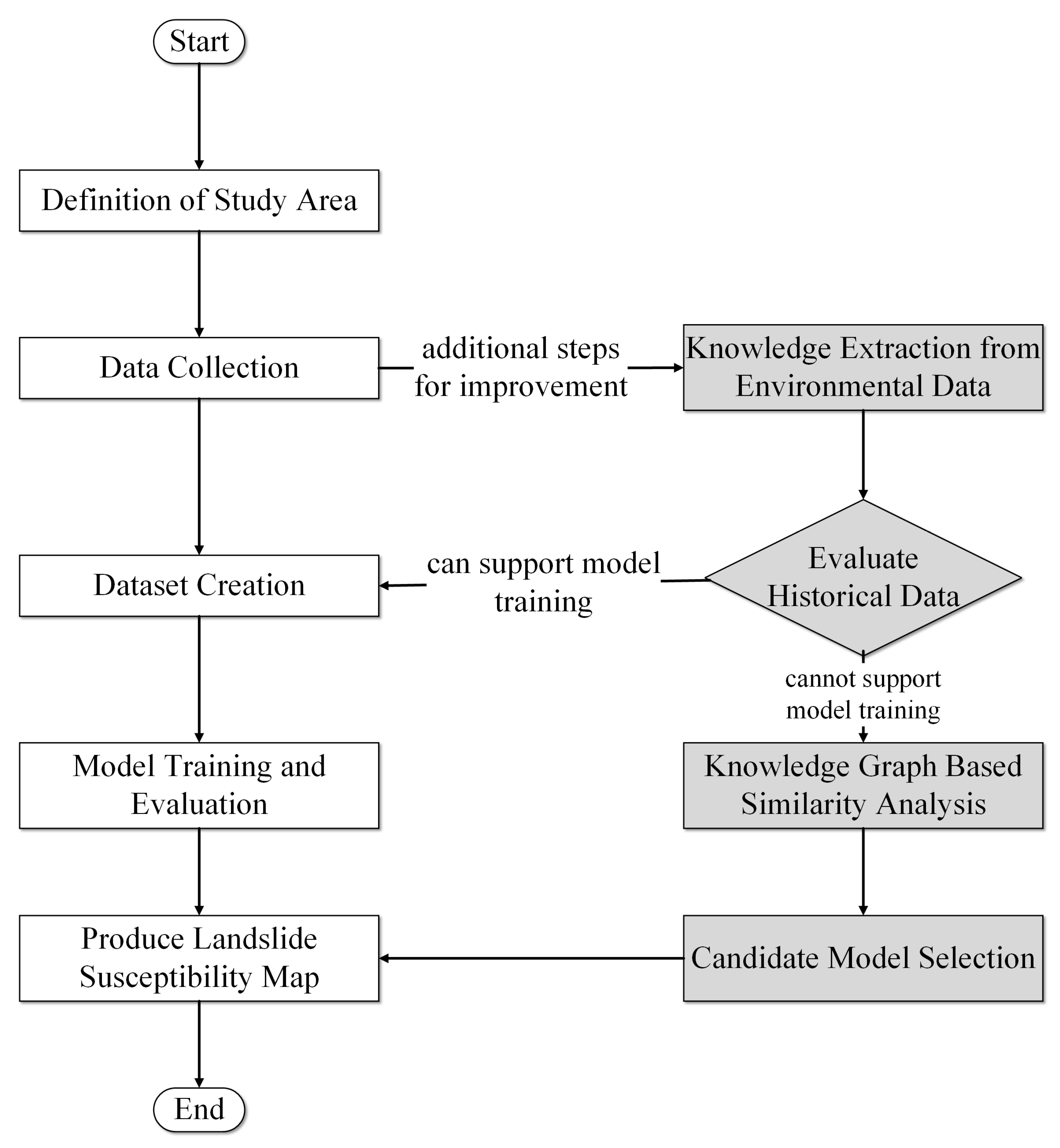
2.1. Workflow for Landslide Prediction

Generally, when using machine learning models for landslide prediction, it is necessary to first define the boundary of the area for landslide prediction. Secondly, data related to landslides, including historical landslide data and environmental data in the area, are collected by means of remote sensing techniques or fieldwork. Based on these data, datasets are created. The dataset contains the environmental features, i.e., causative factors, that need to be input to the model, and the landslide prediction results, i.e., labels, that are output from the model. Then, the parameters of the model are trained based on the dataset. After training, the optimal model is obtained, and the prediction performance is evaluated based on the model. Eventually, the landslide is predicted based on the model.
To improve the effectiveness of landslide prediction in areas with scarce samples, we introduce knowledge graph into the workflow of machine-learning-based landslide prediction. Firstly, as in the general workflow, we define the boundary of the area to be evaluated and collect historical landslide data and environmental data from the area. Secondly, environmental data are structured knowledge and imported into a knowledge graph, i.e., extracting knowledge from environmental data. Then, we evaluate whether the quantity of historical landslide data can support the training of the model. If it can, the subsequent steps are performed following general machine learning methods, including producing the dataset of the area, training the model, and predicting landslides. If the quantity of the historical landslide data cannot support the training of the model, the environmental similarity within the area is analyzed based on the knowledge graph. Finally, the model with the highest similarity to the study area is selected among the candidate models for landslide prediction. Figure 1 shows the difference between the general workflow and the workflow using the knowledge graph.

2.2. Design of Spatio-Temporal Knowledge Graph for Landslide Prediction
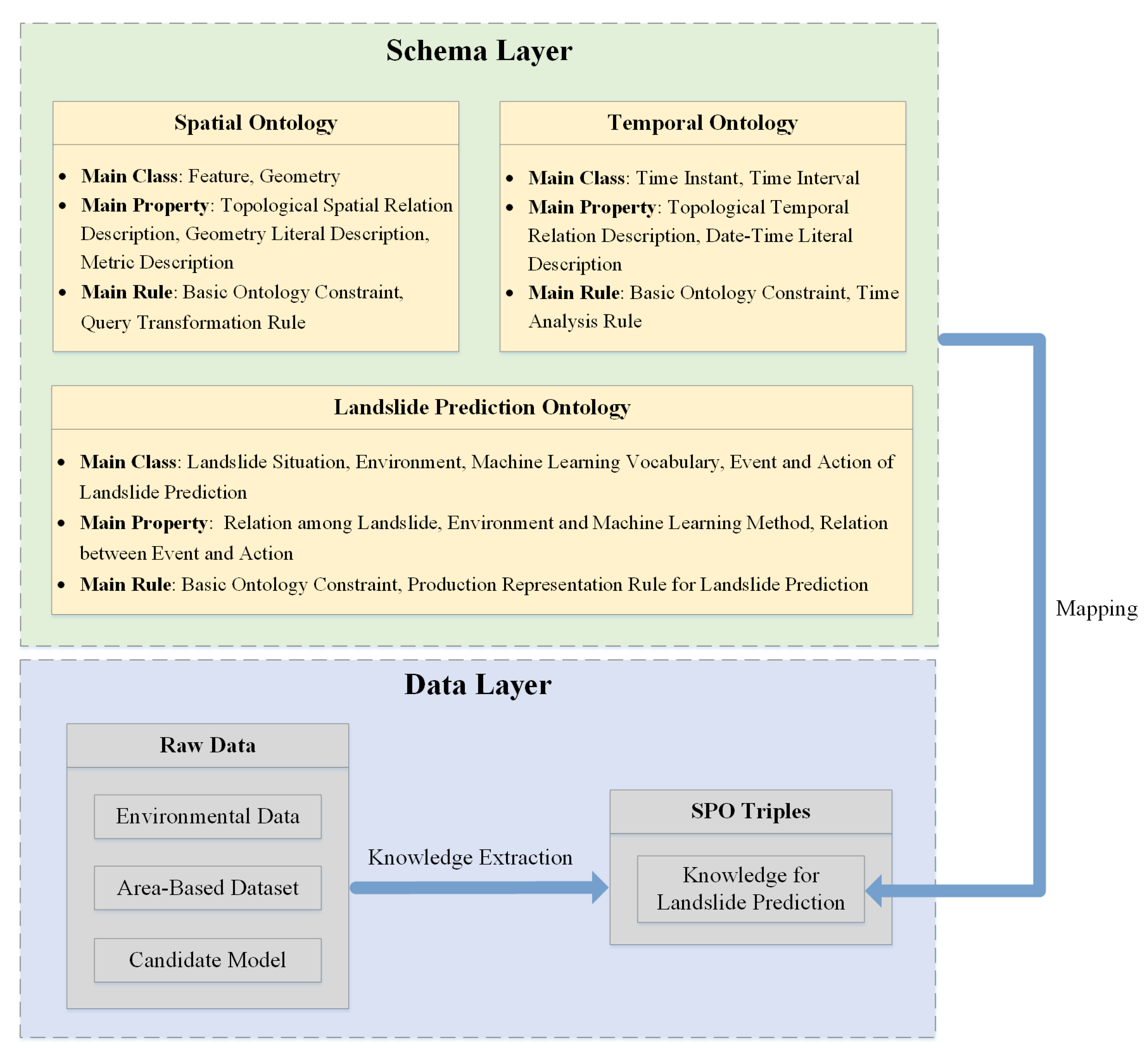
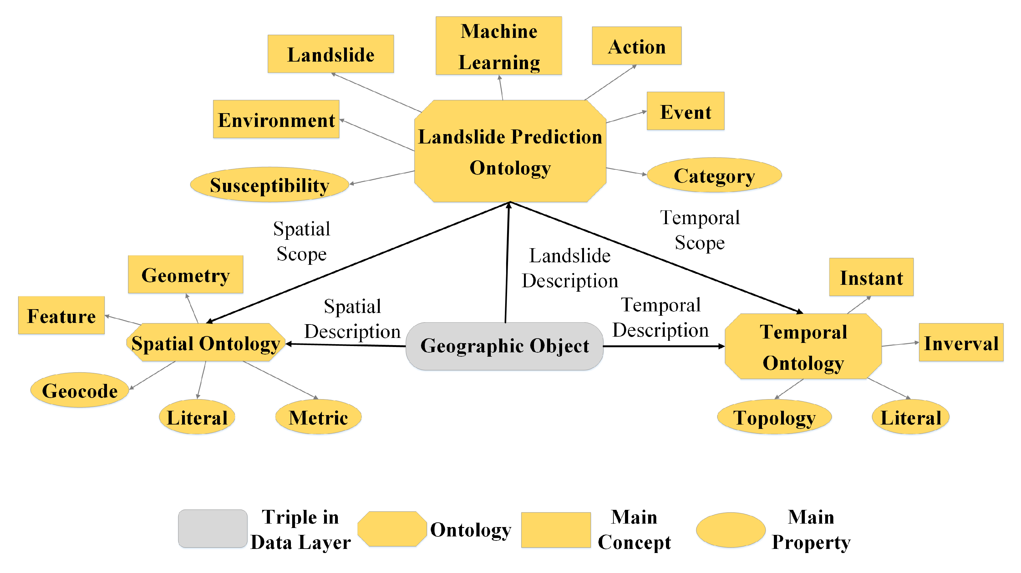
In this paper, we use the spatio-temporal knowledge graph to organize remote sensing environmental data, machine learning models and datasets of the study area. The spatio-temporal knowledge graph includes the schema layer and the data layer, as shown in Figure 2.

2.2.1. Schema Layer

The schema of the knowledge graph is used to describe and organize the spatio-temporal data related to landslides and to define the rules for landslide prediction. We implement the schema using ontologies, which include a spatial ontology, a temporal ontology, and a landslide prediction ontology. Each ontology defines classes, properties, and rules. The classes and properties describe the concepts and their relations involved in landslide prediction, while the rules use classes and properties as symbols to describe the process of spatio-temporal analysis and landslide prediction. The structure of the schema, as well as the main ontologies, concepts, and attributes used, are shown in Figure 3.
  • Spatial ontology
The spatial ontology is used to describe the spatial information of geographic objects and is constructed based on the GeoSPARQL ontology [25]. Geocoding rules are designed in the spatial ontology to serve as the location index of the geographic object.
The classes of the spatial ontology mainly introduce two subclasses of geographic objects in the GeoSPQRQL ontology: the feature class and the geometry class. The spatial terms defined based on the feature and geometry classes can be helpful in modeling geospatial data.
The properties of the spatial ontology mainly define the topological spatial relations between geographic objects, as well as the geometry literal [26], which is the serialization standard used when generating geometry descriptions and the supported geometry types. In addition, the properties of the spatial ontology also include Metric [26], which are scalar spatial properties that describe the geographic object. The main rule of the spatial ontology includes basic ontology constraints for class and property, such as constraints on hierarchical relationships between classes and constraints on property values. The core rule includes rules defined in the GeoSPARQL ontology, such as the query transformation rule for computing spatial relations between geographic objects based on their geometries [25].
In addition, indexable location information helps to improve the efficiency of spatial analysis. However, remote sensing data describe spatial information with latitude and longitude coordinates, which cannot be objectified and indexed. To solve this problem, we designed a geographic tile-based spatial indexing rule, i.e., geocode. Figure 4 illustrates an example of geocoding.
Geocode converts the coordinate properties of geographic objects into tile-coded entities according to the Web Mercator rules [27], i.e., the tile number of the Web Mercator coordinate system is used, instead of the latitude and longitude coordinate system, as the unit to describe the location of the geographic entity. Each tile number consists of the horizontal coordinates, vertical coordinates and zoom level of the tile. The conversion rules are as follows:
x = l o n + 180 360 · 2 z
y = ( 1 ln ( tan ( l a t · π 180 ) + 1 cos ( l a t · π 180 ) ) π ) · 2 z 1
where l o n and l a t denote the entered longitude coordinate and the entered latitude coordinate, x denotes the tile horizontal coordinate after conversion, y denotes the vertical coordinate after conversion, z denotes the zoom level of the tile. Each tile in the geocode represents a set of latitude and longitude coordinates, and tiles with different zoom levels contain different amounts of latitude and longitude coordinates. The higher the zoom level, the fewer the number of latitude and longitude coordinates in a tile, and the more accurate the spatial description of the geographic object.
  • Temporal ontology
The temporal ontology is used to describe the temporal information of geographic objects, and we construct it based on the OWL-Time ontology [28].
The classes of the temporal ontology mainly define the instant and interval to describe the temporal position and duration of the geographic object. The properties of the temporal ontology mainly define the topological temporal relations between geographic objects, such as “meets”, “overlaps” and “during”, developed by Allen [29]. The temporal ontology also defines the Date–Time Literal, which is a serialization standard describing time. Similar to the spatial ontology, the main rule of the temporal ontology includes basic ontology constraints for classes and properties. Additionally, the main rule includes rules defined in the OWL-Time ontology. For example, OWL-Time defines time analysis rules for computing temporal relations between geographic objects based on their time instant and time interval [28].
  • Landslide prediction ontology
The Landslide Prediction Ontology is used to describe the concepts needed for landslide prediction, the relations between concepts, and the reasoning process of landslide prediction.
The classes of the ontology define concepts that describe the landslide situation, such as the severity of the landslide and the phase it is in. Since the environment is the root cause of landslides, the classes also define concepts describing the environment, including the natural environment and the social environment. Additionally, concepts related to machine learning are defined in the classes, such as vocabulary to describe the features of models and datasets. Furthermore, the process of landslide prediction is divided into several events and actions; hence, we also need to define the events and actions involved in landslide prediction in the Landslide Prediction Ontology. For example, when selecting the best model for an area, candidate models are described in the ontology by defining classes.
The properties of the ontology mainly define the relations among landslides, the environment, and machine learning methods, such as describing which environmental factors are causative factors for landslides and which causative factors are used as features of the dataset. The Landslide Prediction Ontology also defines the relations between events and actions in the landslide prediction process. For example, when the environmental similarity between areas is calculated, the result triggers the action of model selection. The relation of this “trigger” is described as a property.
The main rule of the ontology includes basic ontology constraints for class and property. Meanwhile, based on the classes and properties of the Landslide Prediction Ontology, we use the production representation to define a series of rules to describe the process of remote sensing data-driven landslide prediction. This includes the calculation method of environmental similarity, the process of model selection, and the process of landslide prediction.

2.2.2. Data Layer

The data layer consists of subject–predicate–object (SPO) triples, where subjects and objects represent entities in the knowledge graph, and predicates denote the edges connecting them. The raw data include three types of independent data: environmental data, area-based dataset, and candidate model.
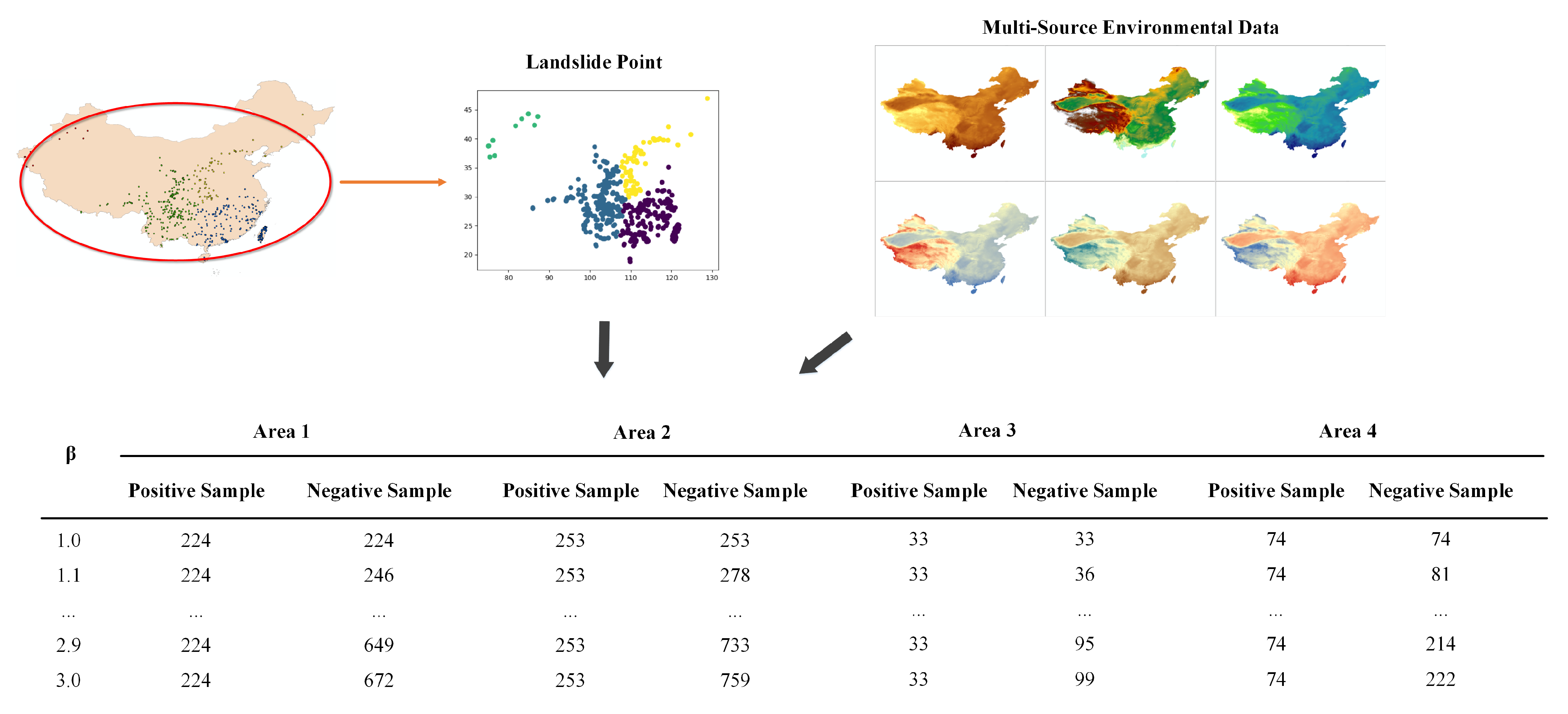
  • Environmental Data: Environmental data record the causative factors of landslides in the area, with each type of environmental data corresponding to a specific causative factor. We extract both the environmental data and the environmental features in the area to generate SPO triples, which are used as the basis for analyzing environmental similarities between areas.
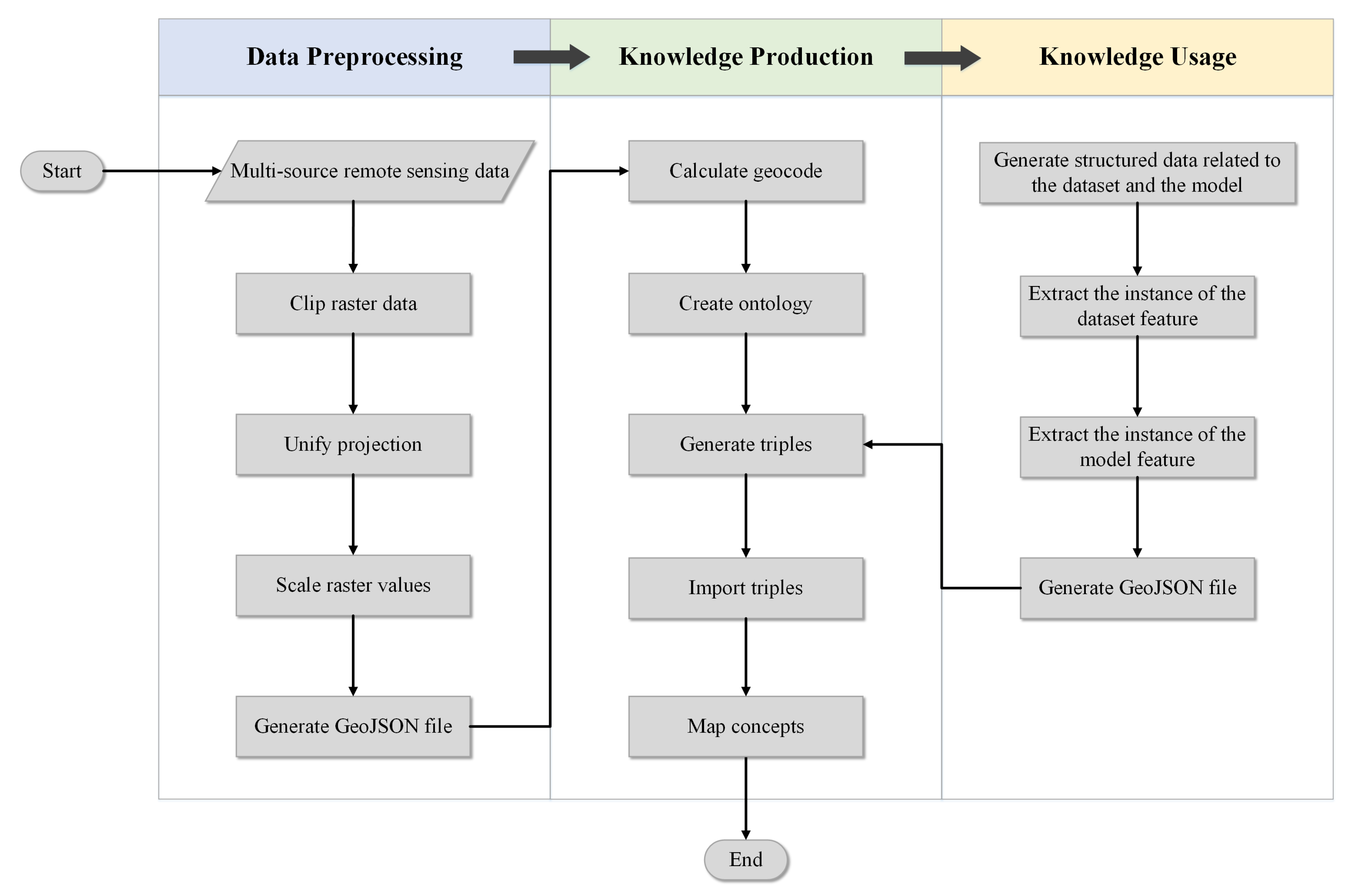
  • Area-based Dataset: Area-based dataset refers to the dataset used for model training in specific areas. During the knowledge extraction process, we extract instances of dataset features to generate SPO triples. The features of the dataset include the number of samples, the sample area, and the statistical parameters of the causative factors contained in the samples.
  • Candidate Model: Candidate model is the model trained based on the area-based dataset. We extract instances of model features to generate SPO triples, which include the name of the model, the address of the parameters, and the name of the samples used for model training.
After generating SPO triples in the data layer, the schema layer relates and organizes these triples to form knowledge that is useful in landslide prediction.

2.3. Landslide Prediction Using Spatio-Temporal Knowledge Graph

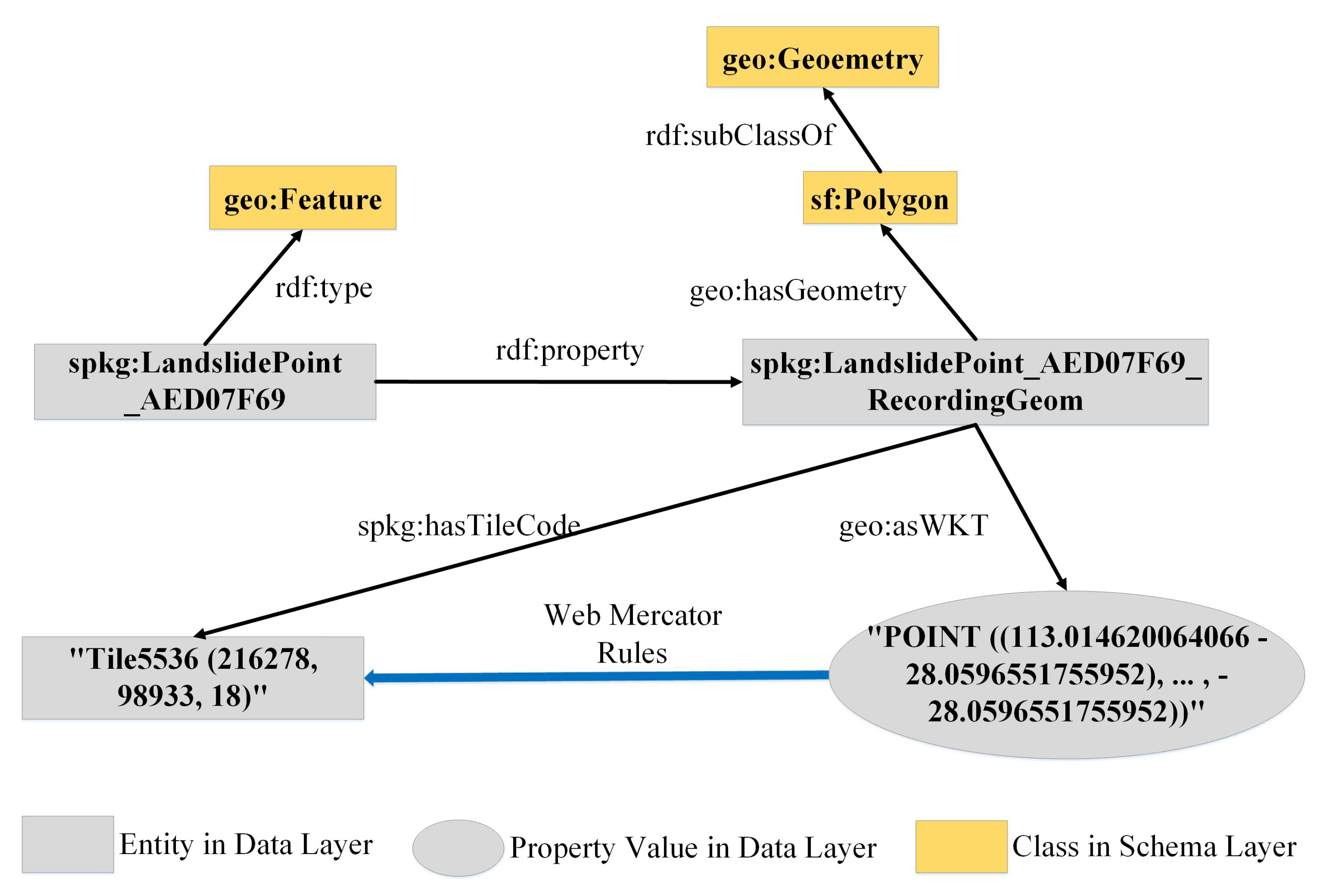
2.3.1. Knowledge Extraction and Storage

When processing environmental data, it is essential to extract and store knowledge while constructing a knowledge graph. After preprocessing the remote sensing monitoring data, they pass through the steps designed to generate knowledge. Simultaneously, data associated with the dataset and the machine learning model are produced by utilizing knowledge, and these data undergo a series of steps to generate corresponding knowledge that helps optimize the results of landslide prediction. The process of transforming data into knowledge is depicted in Figure 5.
  • Data preprocessing
Remote sensing monitoring data quantify environmental elements by assigning a value to each pixel, such as the elevation in DEM data. Since knowledge in a knowledge graph is based on object representation, we convert discrete features in remote sensing data into attributes in objects. The GeoJSON file uses a feature object-based storage mode, which is more conducive to knowledge graph reading than remote sensing data. We preprocess the data and convert the original multi-source remote sensing data into a GeoJSON file that describes the distribution of environmental elements in the study area. After generating the GeoJSON file, we classify adjacent pixels in the remote sensing data with the same environmental element value into the same feature object.
Typically, remote sensing monitoring data of different environmental elements have different spatial ranges. Therefore, in the data preprocessing stage, we need to crop the original remote sensing data to obtain the remote sensing data within the spatial range of the research area. Additionally, remote sensing data from different sources may use different projected coordinate systems, so we must convert multi-source remote sensing data into the same projected coordinate system. We also scale the raster values, which may be decimal, to an integer by multiplying and rounding them. Finally, we generate a GeoJSON file by converting the raster data into vector data and then converting the vector data into the GeoJSON format. During the conversion process, we ensure that the original raster value is restored. The entire process can be automated using the GDAL library [30].
  • Knowledge production
After data preprocessing, a GeoJSON file is generated, followed by the process of knowledge production. First, geocoding is calculated based on the spatial information of each object in the GeoJSON file. Next, SPO triples are generated to describe geographic entity attributes based on the GeoJSON file. The objects in the GeoJSON file correspond to the subjects in the SPO triples, the keys of the object properties correspond to the predicates in the SPO triples, and the values of the object properties correspond to the objects in the SPO triples. In this process, geocoding is also generated as an attribute of geographic entities in the form of SPO triples.
Next, we import the generated SPO triples into the knowledge graph. If the SPO triples are imported for the first time, the ontology needs to be created according to the ontology structure in the schema layer we designed. Spatial ontology and temporal ontology can be directly used as basic ontologies. For the landslide prediction ontology, we use Protégé [31] to define the Class, property, and rule in the ontology. Protégé is a tool that helps users quickly create and edit ontologies. The landslide prediction ontology edited with Protégé can be directly imported into the knowledge graph. In this paper, Virtuoso [32] is used to store ontologies and SPO triples. After importing the ontology and SPO triples, we map the SPO triples of the data layer and the ontology of the schema layer to generate semantic associations between data features to produce knowledge.
  • Knowledge usage
During the process of knowledge usage, additional structured data related to the dataset and the machine learning model are generated, which also need to be extracted and stored in the knowledge graph. We extract instances of features from the dataset and the model, and write them into a GeoJSON file. The description objects of the dataset and the model are areas, and the characteristics of the dataset and the model in different areas are different. In the GeoJSON file, an area is defined as a feature object. The geometry of the feature describes the location of this area, and the properties of the feature represent the instance of the dataset feature and the model feature. After generating the GeoJSON file, we follow the steps of knowledge production to generate and import SPO triples. We map the SPO triples to schema layer ontologies to produce knowledge related to domain models and datasets.

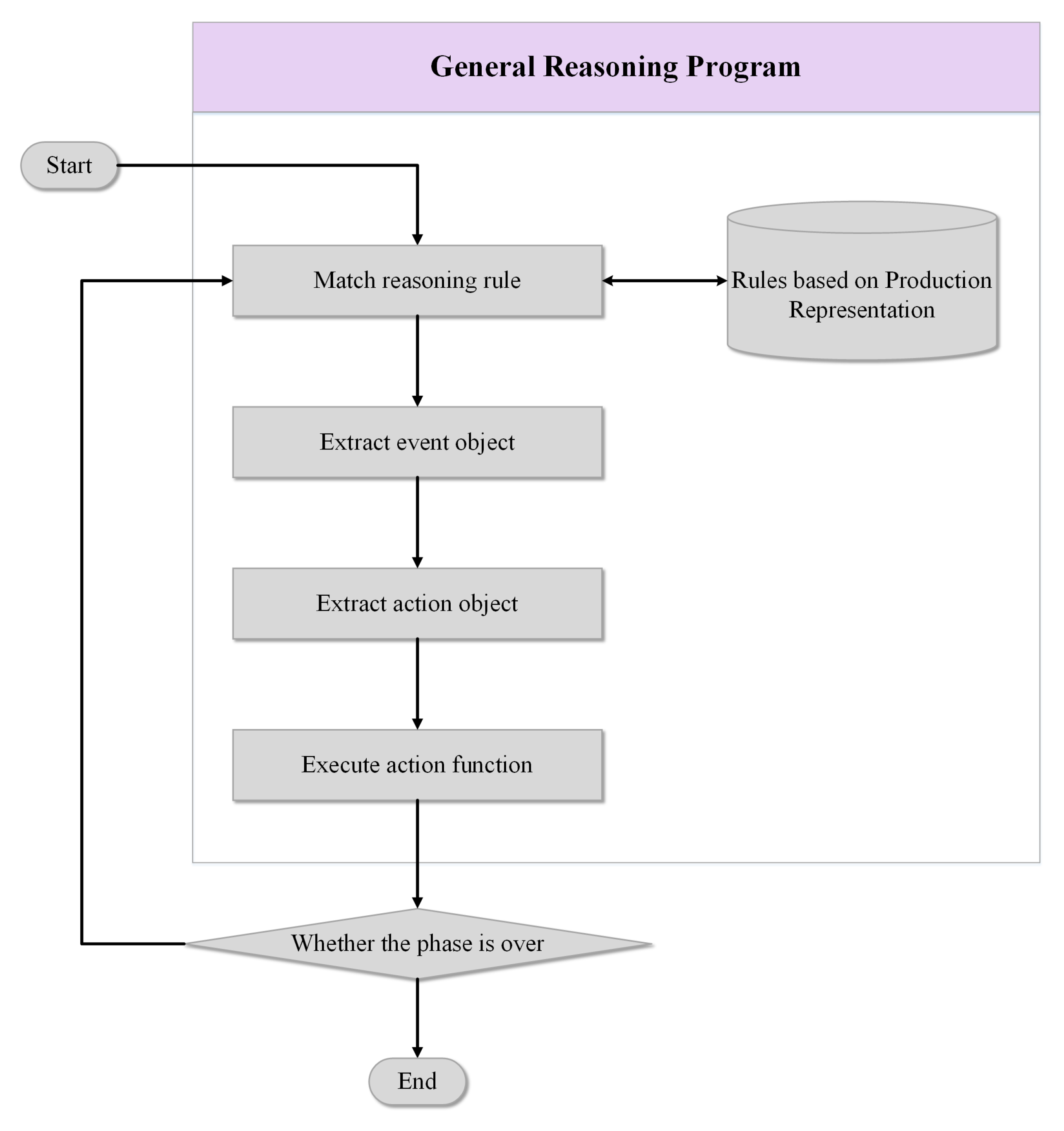
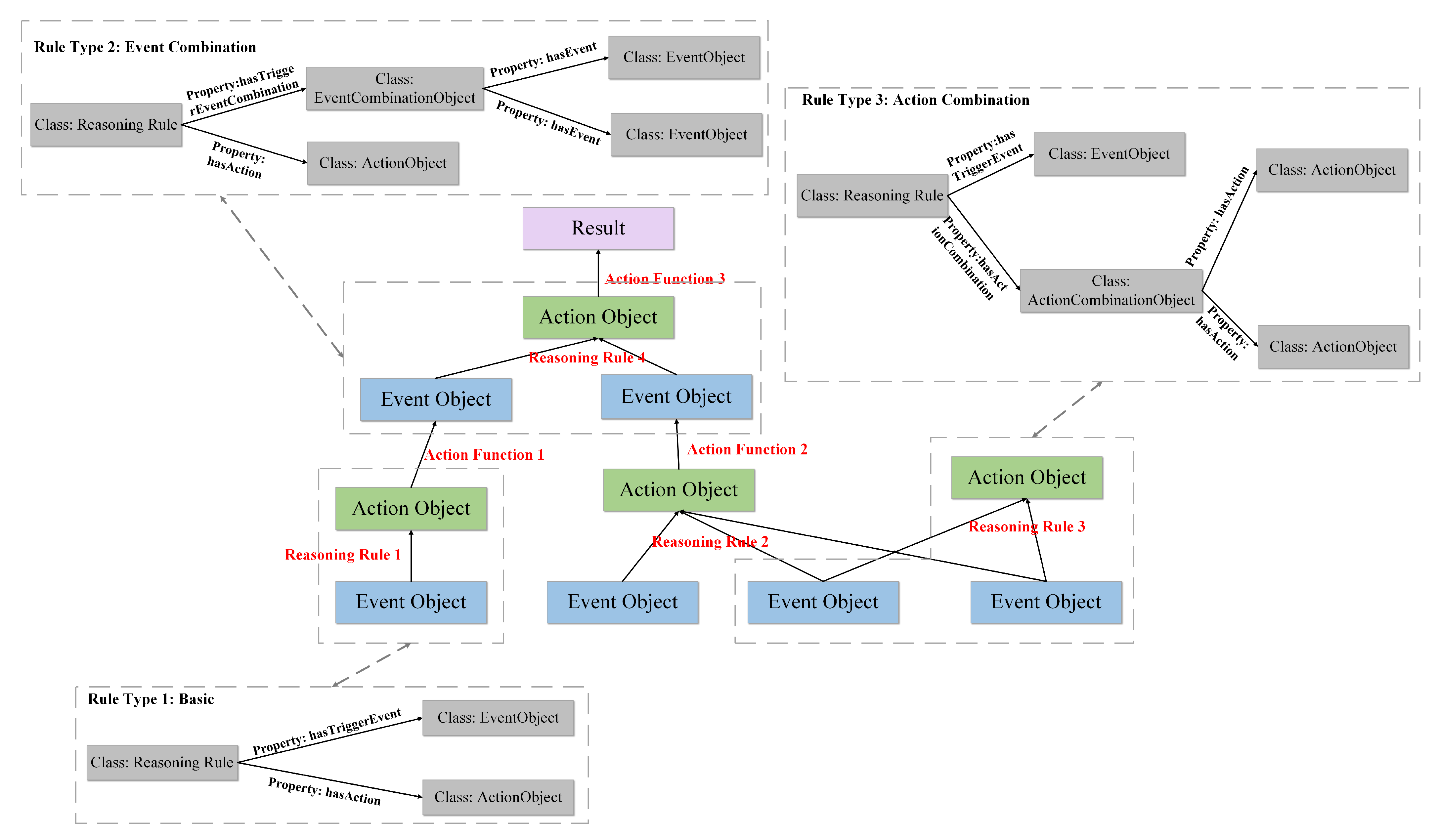
2.3.2. Semantic Reasoning

Semantic reasoning is based on the production representation and recommends models for areas with sparse samples while following the main rule in the schema. It consists of two phases, similarity analysis and candidate model selection, each with several production rules. The general reasoning program automatically performs semantic reasoning as shown in Figure 6. A rule is triggered by an event object, and the corresponding action function is executed to generate a result based on the defined action object. The generated result then triggers the execution of other rules in the rule set until the phase is complete. Figure 7 shows the template defining this process.
The Jaccard index is used to evaluate the similarity of the environment between the area. The equation is as follows:
J ( A , B ) = | A B | | A | + | B | | A B |
where A and B denote the environmental feature collection of area A and area B, and the larger the Jaccard index, the more similar the environment of the two areas.
The Jaccard index essentially compares the number of environmental features that are similar between areas. For discrete environmental features, the mode of the feature values within the area is taken as the environmental feature value representing that area. If the environmental feature values representing two areas are equal, then this environmental feature is considered similar in the two areas. For continuous environmental features, the average of the feature values within the area is taken as the environmental feature value representing that area. For area A and area B, the similarity of the environmental features in the two areas is determined according to the following equation:
i s S i m i l a r = Y e s | F A F B | F m a x F m i n N A + N B N o | F A F B | > F m a x F m i n N A + N B
where F A and F B denote the environmental feature values representing area A and area B, F m a x and F m i n denote the maximum and minimum values that can be obtained for the environmental feature, N A denotes the number of the values of this feature in area A, and N B denotes the number of the values of this feature in area B.
The statistical parameters calculated by the similarity analysis are stored as properties in the triples generated from the area-based dataset. When predicting landslides in study areas with sparse samples, the statistical parameters of the study area are first calculated. Then, a similarity analysis is performed based on the statistical parameters. Eventually, the area with the most similar environmental features to the study area is selected from the knowledge graph, and the model trained from the dataset of that area is obtained through a semantic query, i.e., the process of candidate model selection.

3. Experiment and Result
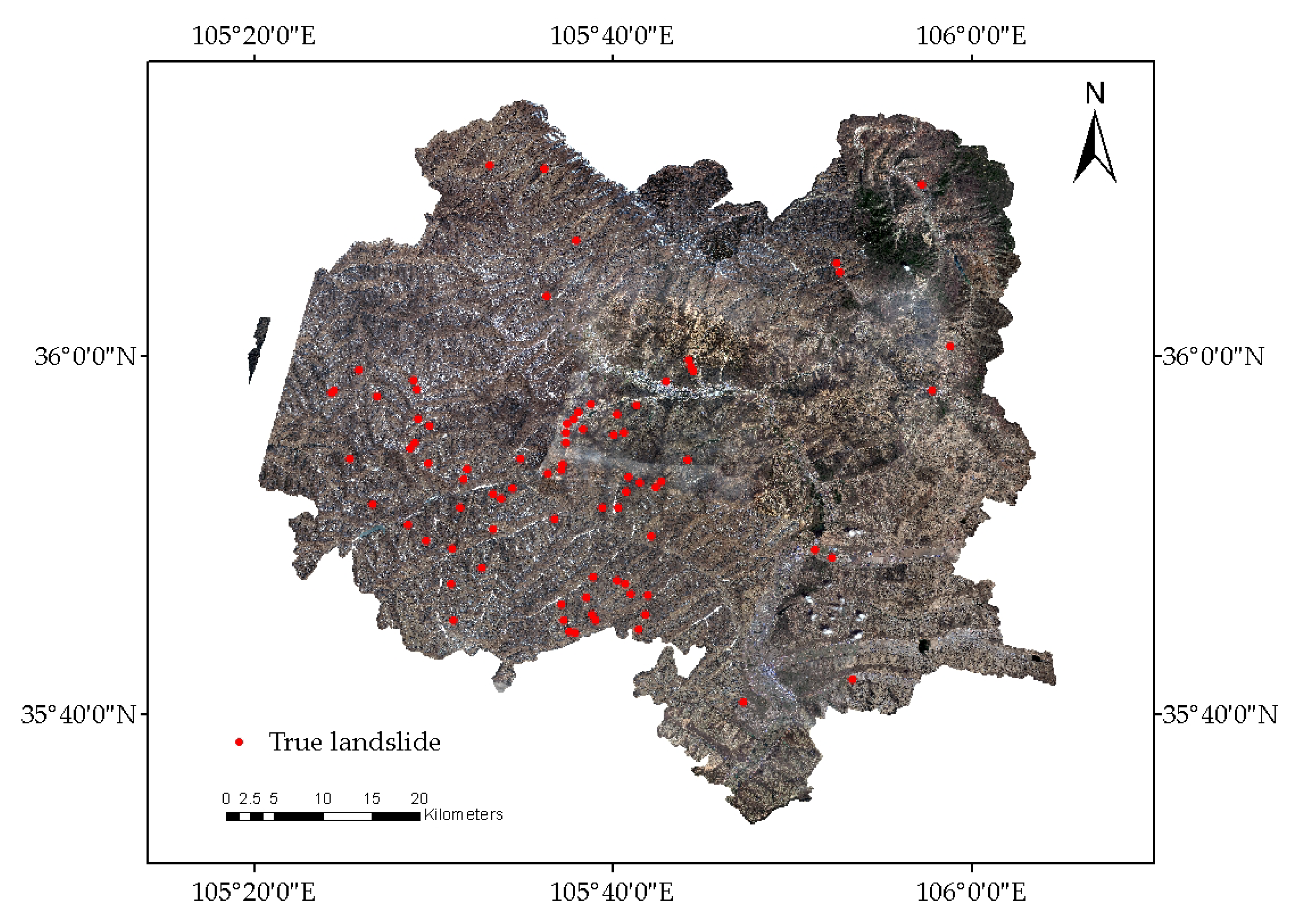
3.1. Study Area

We obtained historical landslide data for China from the Global Landslide Catalog [33]. China is one of the countries in the world with the highest frequency of landslide hazards, posing threats to both the ecological environment and the safety of people and their property. Furthermore, China is situated at the intersection of continental plates, and its mountainous areas account for nearly 70% of the land area, with a highly undulating terrain that provides natural conditions for landslides to occur.
To demonstrate the effectiveness of our method, we applied the DBSCAN algorithm [34] to cluster landslide points based on their spatial locations. Landslide points belonging to the same category are indicated in the same area, resulting in four simulated study areas, denoted as area 1, area 2, area 3, and area 4. Among them, area 3 and area 4 have the smallest sample sizes and can be simulated as sample scarcity cases. Then, environmental data were collected as causative factors for the training of machine learning models. Table 1 shows the sources and details of the experimental data, and Figure 8 depicts the process of obtaining samples from the experimental data for the four areas.
Additionally, although the selected simulated area can demonstrate the advantages of our method in terms of effectiveness, it is difficult to show the actual prediction results because the simulated area does not have clear boundaries. Therefore, we validated the practical effectiveness of our method using landslide data from Xiji County, located in the southern part of Ningxia Province, China. Xiji County has an area of approximately 1581.5 square kilometers, ranging from 35°35 to 36°14 north latitude and 105°20 to 106°04 east longitude. We obtained 82 landslide events, which mainly occurred in areas with broken topography and narrow ridges. We used the environmental data in Table 1 to create samples, but due to the scarcity of samples, it is difficult for conventional machine learning methods to make accurate predictions. The distribution of landslide points and the boundary of Xiji County are shown in the Figure 9.

3.2. Machine Learning Model

The performance of four methods, SVM [43], RF [44], KNN [45], and GCF [46], was compared based on landslide prediction research. To assess the landslide prediction, the landslide and non-landslide samples are both randomly divided into two parts: samples for model training and samples for performance testing.
  • Support Vector Machine: The SVM algorithm is a supervised learning binomial classifier based on the risk minimization principle of structured architecture. It can accurately deal with complex nonlinear boundary models.
  • Random Forest: The RF algorithm is a combination algorithm based on the classification and regression tree (CART) proposed by Breiman. By randomly selecting k samples from the training set and putting them back into the ground, a decision tree corresponding to the training samples is generated; thus, a random forest composed of k decision trees is generated. According to the prediction result of each tree, the final prediction result is obtained according to the category with the most votes.
  • K-Nearest Neighbors: The KNN algorithm is a supervised machine learning classification algorithm. In the K-nearest neighbor method, the K value and distance measure are determined in advance, and the training set and test set are prepared in advance. Through the training set, the feature space is divided into subspaces, and every sample in the training set occupies a part of a space.
  • Multigraded Cascade Forest: The GCF algorithm is a supervised ensemble learning method that combines the theory of random forests and a deep neural network. The GCF is composed of a multilevel random forest model, and each level of the random forest model contains many different types of random forests. This multilevel and multidimensional random forest processes the probabilistic eigenvector of the input data, and can effectively enhance the performance of the prediction algorithm for the input data and help to improve the prediction accuracy. Each stage uses the output of the upper stage and the original probability feature vector as its input; that is, it uses the feature information after the upper stage is processed, combined with the original probability feature vector. The new information is processed at this level and passed on to the next level.

3.3. Metrics

The process of landslide prediction based on machine learning is a binary classification process for landslide and non-landslide points. Several measures, including precision, recall and the F1 index, are employed to evaluate the overall landslide prediction accuracy for model comparisons. The equations of precision, recall, and F1 index are shown below:
P r e c i s i o n = T P T P + F N
R e c a l l = T P T P + F P
F 1 = 2 P r e c i s i o n R e c a l l P r e c i s i o n + R e c a l l
where T P denotes the number of true positives predicted as being in the positive category; T N denotes the number of true negatives predicted as negatives; F P denotes the number of true negatives predicted as positives; F N denotes the number of true positives predicted as negatives.
Additionally, the Receiver Operating Characteristic (ROC) curve and the Area Under the Curve (AUC) are used to evaluate the results. The horizontal and vertical axes of the ROC curve represent the false positive (FP) rate and true positive (TP) rate, respectively. The AUC is the area under the ROC curve. When the AUC exceeds 0.5, the model is considered to have positive discriminative ability. A higher AUC value, closer to 1, indicates a better predictive performance.

3.4. Experimental Results

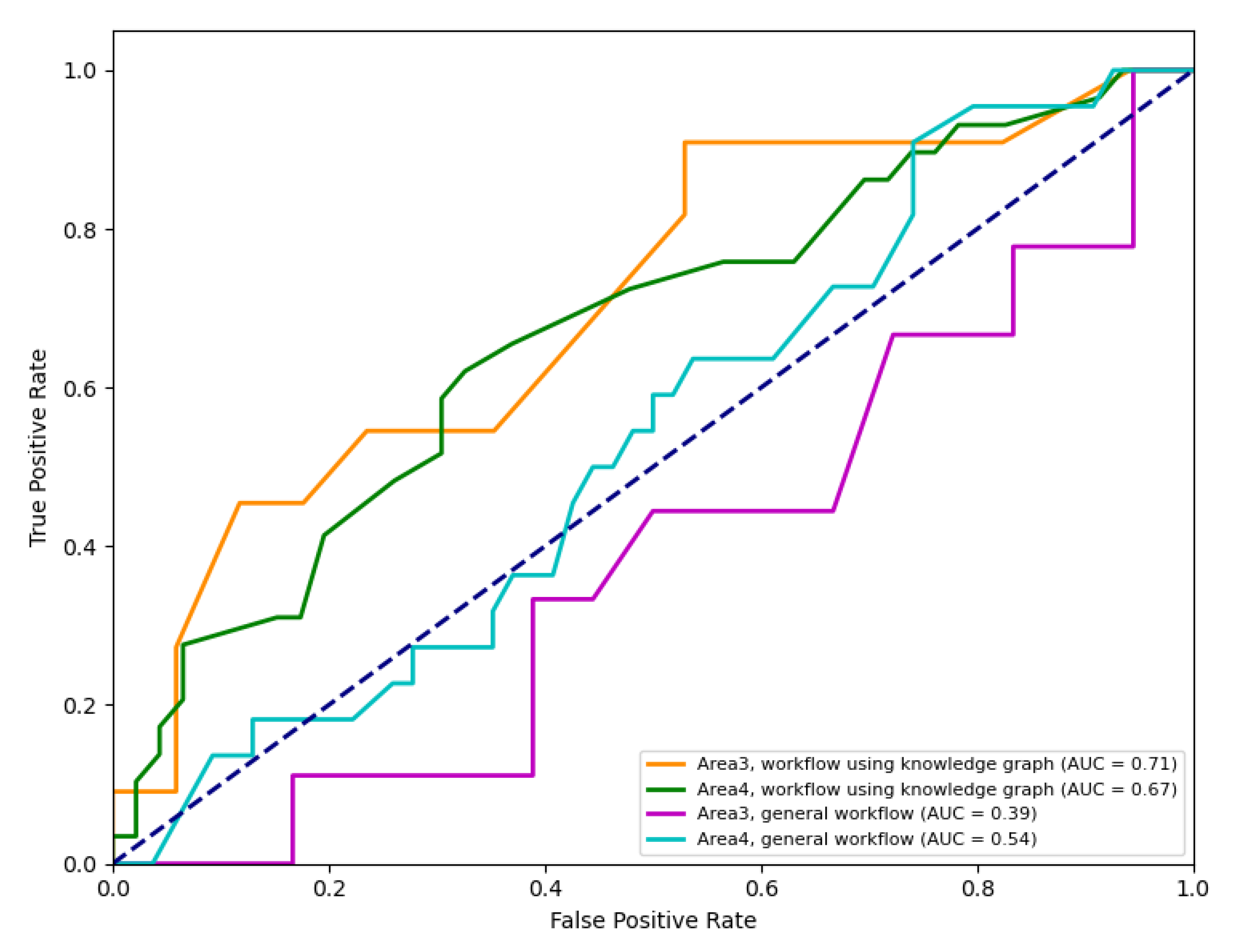
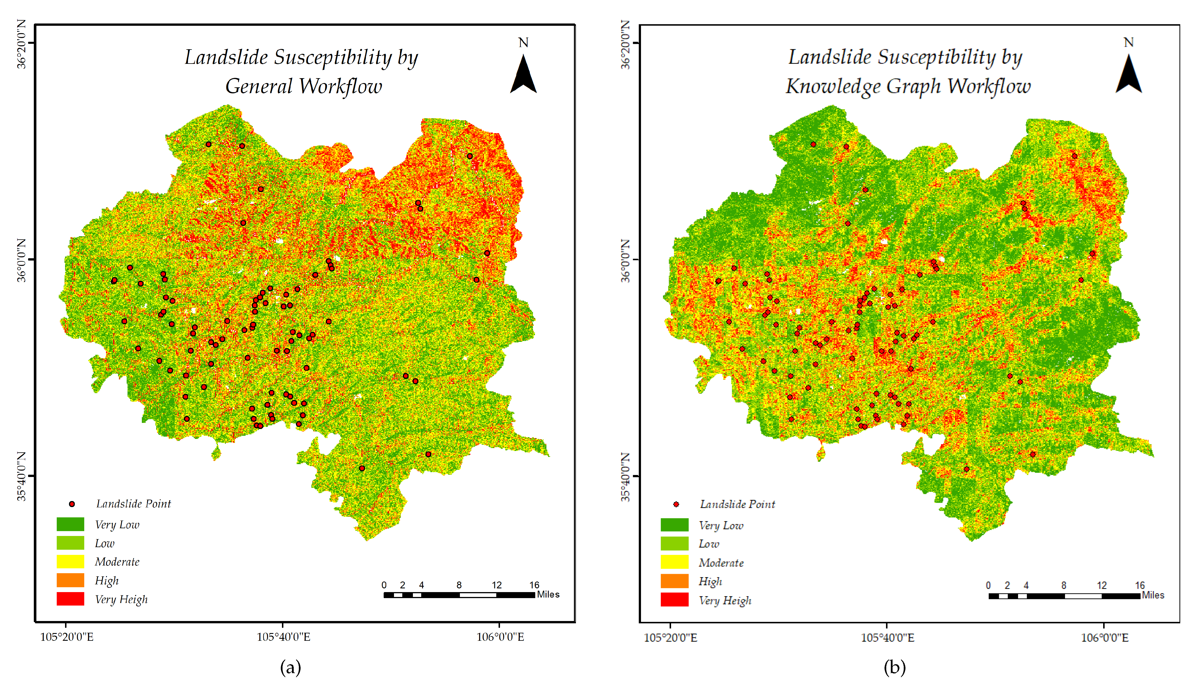
3.4.1. Effectiveness of the Method

Table 2 presents a summary of the results obtained from predicting landslides in four areas using different candidate models. Initially, existing samples of each area were used to predict landslides, and candidate models numbered 1, 2, 3, and 4 were obtained from the training samples of areas 1, 2, 3, and 4, respectively. It was observed that models in areas with sparse samples were generally difficult to fit or had a poor performance after dividing the training and test sets. To address this issue, the environmental similarity (Jaccard Index) between sample-sufficient areas and sample-scarce areas was calculated based on the spatio-temporal knowledge graph’s reasoning rules, and candidate models were selected for landslide prediction. When predicting landslides for area pairs with similar environmental features, using model 2 to predict the landslide of area 3, for instance, reduced the issue of sample scarcity in the prediction process for area 3. It was also noted that a larger Jaccard Index indicated that the environmental features of the two areas were more similar, and the model performed better. In terms of selecting model types, SVM and GCF showed better prediction performance for area 3, while KNN and GCF performed better for area 4. Table 3 presents the optimal performance achieved by predicting sample-sparse areas using the general workflow and the workflow incorporating knowledge graph, while Figure 10 displays the corresponding ROC curves. It is evident that incorporating the knowledge graph into the workflow enhances the predictive capability for sample-scarcity areas. However, it should be noted that the number of candidate models and the limitations of model training knowledge still leave room for improvements in the AUC.
Moreover, we implemented two workflows for landslide prediction using machine learning. In areas with limited samples, the general workflow involves more manual steps. On the other hand, the workflow based on the knowledge graph offers the advantages of automation and faster computation. Table 4 provides a comparison of the two workflows.

3.4.2. Validation in Xiji

To further demonstrate the effectiveness of this method in real-world scenarios, we applied the knowledge graph-based workflow to produce a landslide susceptibility map in Xiji County. Our approach has shown promising results in preliminary studies and we sought to validate it in a practical setting. We first collected environmental data from Xiji County from the sources listed in Table 1. Next, we extracted knowledge from the data and stored it in the knowledge graph, following the data processing process outlined in Figure 5. The knowledge graph performed semantic reasoning to predict landslides, using similarity analysis and candidate model selection as detailed in Section 2.3.2. Based on Equations (3) and (4), the Jaccard index of Area 1 and Xiji is 0.6, and the Jaccard index of Area 2 and Xiji is 0.3. Therefore, the knowledge graph selected the model produced by Area 1 from the candidate models to generate the landslide susceptibility map. Among the candidate models, RF produced the best results for predicting landslide susceptibility in Xiji, with 100 trees in the forest, a minimum of 2 samples required to split an internal node, and a ratio of positive to negative samples of 1.7.
In addition, we followed the general machine learning method shown in Figure 1 to generate the susceptibility map and compared it with our method. The results are presented in Figure 11. Compared to the real landslide sites, the general machine learning method was unable to accurately evaluate the spatial distribution of susceptibility in Xiji County due to the lack of dataset. On the other hand, the method using the knowledge graph workflow mitigated the effect of sample scarcity on the results.

4. Discussion

In our experiments, we conducted both an effectiveness validation and a validation based on real scenarios. For the effectiveness validation, we divided the landslide dataset into four areas, including two sample-sufficient areas and two sample-scarce areas. We then used our proposed knowledge-graph-based method and general machine learning methods to predict the sample-scarce areas. Our method demonstrated several advantages over general machine learning methods, including better precision due to the use of similarity reasoning rules and environmental features stored in the spatio-temporal knowledge graph. The similarity analysis method we designed quantifies the similarity of geographical features, which improves prediction accuracy, as shown in our experiments. Additionally, the knowledge graph accelerated the prediction process by using automatic semantic reasoning rules and the storage advantages of the graph structure, providing a speed advantage over other methods.
Furthermore, for validation based on real scenarios in Xiji County, we further compared the effectiveness of our workflow and a general machine learning workflow to draw susceptibility maps. Our study demonstrated that the proposed workflow can mitigate the problem of poor prediction in sample-scarce areas. Among the candidate models, Random Forest performed the best, likely due to its ability to handle high-dimensional variables without variable deletion and reduce overfitting through the use of multiple trees, substitution methods, and random subset selection to split nodes.
However, it is important to acknowledge that our proposed method has limitations. Firstly, it is sensitive to prediction size, and larger study areas may require longer processing times and more storage space. Secondly, while our method shows promising results, the precision still needs improvement in real scenarios, which may be achieved by using higher-resolution environmental remote sensing data and more comprehensive landslide point records. Lastly, in future experiments, specific model training techniques could be incorporated as knowledge in the knowledge graph to standardize the comparison criteria, and the design of inference rules for model training should be carefully considered.

5. Conclusions

Data-driven methods usually require a sufficient number of samples to train the models. In areas where samples are limited, some studies employed prediction methods based on transfer learning or GANs. However, these methods face challenges in organizing multi-source remote sensing data or face difficulties training, making the munsuitable for disaster scenarios that require real-time prediction. Moreover, the lack of a systematic prediction process and the low level of automation in prediction resulted in low prediction efficiency for landslides. In this paper, we propose a novel approach to improve the performance of remote sensing data-driven landslide prediction, which makes the following main contributions:
  • This paper proposes an efficient method for disaster analysis in the field of geohazard management by combining knowledge-driven and data-driven approaches.
  • The problem of data-driven methods being over-sensitive to data is alleviated by semantic modeling and knowledge fusion.
  • A novel paradigm is defined for the standardized integration of multi-source remote sensing resources, which helps to share and reuse formalized remote sensing resources and demonstrates the potential of spatio-temporal knowledge graphs in the field of remote sensing.
In future research, we will strive to improve the generalization ability of spatio-temporal knowledge graph. On the one hand, we should define the inference rules for machine learning training strategies in the spatio-temporal knowledge graph to improve the prediction accuracy of candidate models. We will also attempt to integrate other data-driven methods, such as representation learning. On the other hand, we will incorporate more disaster knowledge, such as exposure factors and other geological disaster concepts, into the model to assess the comprehensive risk of geological disasters. Additionally, we will pay more attention to the interpretability of landslide prediction methods. By leveraging the structural advantages of knowledge graph, modeling landslide disaster environments based on multi-source remote sensing data helps to explain the inherent features between causative factors and positively contributes to the prediction results of landslides.

Author Contributions

Conceptualization, L.C., L.P. and L.Y.; methodology, L.C., L.P. and W.L.; validation, L.C. and W.L.; resources, L.C.; data curation, L.C. and X.G.; writing—original draft preparation, L.C. and X.G.; writing—review and editing, L.C., X.G. and L.Y.; funding acquisition, L.P. All authors have read and agreed to the published version of the manuscript.

Funding

This work was supported by Ningxia Key R&D Program (2020BFG02013). This work was sponsored by Tianjin intelligent manufacturing special fund project (NO. 20201198).

Data Availability Statement

Data sharing not applicable.

Conflicts of Interest

The authors declare no conflict of interest.

References

  1. Yilmaz, I. Landslide susceptibility mapping using frequency ratio, logistic regression, artificial neural networks and their comparison: A case study from Kat landslides (Tokat—Turkey). Comput. Geosci. 2009, 35, 1125–1138. [Google Scholar] [CrossRef]
  2. Liu, H.; Liu, J.; Chen, J.; Qiu, L. Experimental study on tilting deformation and a new method for landslide prediction with retaining-wall locked segment. Sci. Rep. 2023, 13, 5149. [Google Scholar] [CrossRef] [PubMed]
  3. Capparelli, G.; Versace, P. Analysis of landslide triggering conditions in the Sarno area using a physically based model. Hydrol. Earth Syst. Sci. 2014, 18, 3225–3237. [Google Scholar] [CrossRef]
  4. Mandal, B.; Mandal, S. Analytical hierarchy process (AHP) based landslide susceptibility mapping of Lish river basin of eastern Darjeeling Himalaya, India. Adv. Space Res. 2018, 62, 3114–3132. [Google Scholar] [CrossRef]
  5. Akgun, A.; Dag, S.; Bulut, F. Landslide susceptibility mapping for a landslide-prone area (Findikli, NE of Turkey) by likelihood-frequency ratio and weighted linear combination models. Environ. Geol. 2008, 54, 1127–1143. [Google Scholar] [CrossRef]
  6. Đurić, U.; Marjanović, M.; Radić, Z.; Abolmasov, B. Machine learning based landslide assessment of the Belgrade metropolitan area: Pixel resolution effects and a cross-scaling concept. Eng. Geol. 2019, 256, 23–38. [Google Scholar] [CrossRef]
  7. Ma, Z.; Mei, G.; Piccialli, F. Machine learning for landslides prevention: A survey. Neural Comput. Appl. 2021, 33, 10881–10907. [Google Scholar] [CrossRef]
  8. Chen, W.; Xie, X.; Peng, J.; Wang, J.; Duan, Z.; Hong, H. GIS-based landslide susceptibility modelling: A comparative assessment of kernel logistic regression, Naïve-Bayes tree, and alternating decision tree models. Geomat. Nat. Hazards Risk 2017, 8, 950–973. [Google Scholar] [CrossRef]
  9. Tian, Y.; Xu, C.; Hong, H.; Zhou, Q.; Wang, D. Mapping earthquake-triggered landslide susceptibility by use of artificial neural network (ANN) models: An example of the 2013 Minxian (China) Mw 5.9 event. Geomat. Nat. Hazards Risk 2019, 10, 1–25. [Google Scholar] [CrossRef]
  10. Marjanović, M.; Kovačević, M.; Bajat, B.; Voženílek, V. Landslide susceptibility assessment using SVM machine learning algorithm. Eng. Geol. 2011, 123, 225–234. [Google Scholar] [CrossRef]
  11. Tien Bui, D.; Shirzadi, A.; Shahabi, H.; Geertsema, M.; Omidvar, E.; Clague, J.J.; Thai Pham, B.; Dou, J.; Talebpour Asl, D.; Bin Ahmad, B.; et al. New ensemble models for shallow landslide susceptibility modeling in a semi-arid watershed. Forests 2019, 10, 743. [Google Scholar] [CrossRef]
  12. Pham, B.T.; Prakash, I.; Dou, J.; Singh, S.K.; Trinh, P.T.; Tran, H.T.; Le, T.M.; Van Phong, T.; Khoi, D.K.; Shirzadi, A.; et al. A novel hybrid approach of landslide susceptibility modelling using rotation forest ensemble and different base classifiers. Geocarto Int. 2020, 35, 1267–1292. [Google Scholar] [CrossRef]
  13. Dou, J.; Yunus, A.P.; Bui, D.T.; Merghadi, A.; Sahana, M.; Zhu, Z.; Chen, C.W.; Han, Z.; Pham, B.T. Improved landslide assessment using support vector machine with bagging, boosting, and stacking ensemble machine learning framework in a mountainous watershed, Japan. Landslides 2020, 17, 641–658. [Google Scholar] [CrossRef]
  14. Hong, H.; Liu, J.; Bui, D.T.; Pradhan, B.; Acharya, T.D.; Pham, B.T.; Zhu, A.X.; Chen, W.; Ahmad, B.B. Landslide susceptibility mapping using J48 Decision Tree with AdaBoost, Bagging and Rotation Forest ensembles in the Guangchang area (China). Catena 2018, 163, 399–413. [Google Scholar] [CrossRef]
  15. Al-Najjar, H.A.; Pradhan, B.; Sarkar, R.; Beydoun, G.; Alamri, A. A new integrated approach for landslide data balancing and spatial prediction based on generative adversarial networks (GAN). Remote Sens. 2021, 13, 4011. [Google Scholar] [CrossRef]
  16. Zhu, Q.; Chen, L.; Hu, H.; Pirasteh, S.; Li, H.; Xie, X. Unsupervised feature learning to improve transferability of landslide susceptibility representations. IEEE J. Sel. Top. Appl. Earth Obs. Remote Sens. 2020, 13, 3917–3930. [Google Scholar] [CrossRef]
  17. Ai, X.; Sun, B.; Chen, X. Construction of small sample seismic landslide susceptibility evaluation model based on Transfer Learning: A case study of Jiuzhaigou earthquake. Bull. Eng. Geol. Environ. 2022, 81, 116. [Google Scholar] [CrossRef]
  18. Gutierrez, C.; Sequeda, J.F. Knowledge graphs. Commun. ACM 2021, 64, 96–104. [Google Scholar] [CrossRef]
  19. Chen, X.; Jia, S.; Xiang, Y. A review: Knowledge reasoning over knowledge graph. Expert Syst. Appl. 2020, 141, 112948. [Google Scholar] [CrossRef]
  20. Singhal, A. Introducing the knowledge graph: Things, not strings. Off. Google Blog 2012, 5, 16. [Google Scholar]
  21. Nayyeri, M.; Vahdati, S.; Khan, M.T.; Alam, M.M.; Wenige, L.; Behrend, A.; Lehmann, J. Dihedron Algebraic Embeddings for Spatio-Temporal Knowledge Graph Completion. In Proceedings of the European Semantic Web Conference, Crete, Greece, 29 May–2 June 2022; Springer: Cham, Switzerland, 2022; pp. 253–269. [Google Scholar]
  22. Ge, X.; Yang, Y.; Peng, L.; Chen, L.; Li, W.; Zhang, W.; Chen, J. Spatio-temporal knowledge graph based forest fire prediction with multi source heterogeneous data. Remote Sens. 2022, 14, 3496. [Google Scholar] [CrossRef]
  23. Wang, S.; Zhang, X.; Ye, P.; Du, M.; Lu, Y.; Xue, H. Geographic knowledge graph (GeoKG): A formalized geographic knowledge representation. ISPRS Int. J. Geo-Inf. 2019, 8, 184. [Google Scholar] [CrossRef]
  24. Yan, B.; Janowicz, K.; Mai, G.; Gao, S. From itdl to place2vec: Reasoning about place type similarity and relatedness by learning embeddings from augmented spatial contexts. In Proceedings of the 25th ACM SIGSPATIAL International Conference on Advances in Geographic Information Systems, Redondo Beach, CA, USA, 7–10 November 2017; pp. 1–10. [Google Scholar]
  25. Battle, R.; Kolas, D. Enabling the geospatial semantic web with parliament and geosparql. Semant. Web 2012, 3, 355–370. [Google Scholar] [CrossRef]
  26. Car, N.J.; Homburg, T. GeoSPARQL 1.1: Motivations, Details and Applications of the Decadal Update to the Most Important Geospatial LOD Standard. ISPRS Int. J. Geo-Inf. 2022, 11, 117. [Google Scholar] [CrossRef]
  27. Battersby, S.E.; Finn, M.P.; Usery, E.L.; Yamamoto, K.H. Implications of web Mercator and its use in online mapping. Cartogr. Int. J. Geogr. Inf. Geovis. 2014, 49, 85–101. [Google Scholar] [CrossRef]
  28. Time Ontology in OWL. Available online: https://www.w3.org/TR/owl-time/ (accessed on 8 August 2022).
  29. Allen, J.F.; Ferguson, G. Actions and events in interval temporal logic. J. Log. Comput. 1994, 4, 531–579. [Google Scholar] [CrossRef]
  30. Westra, E. Python Geospatial Development; Packt Publishing: Birmingham, UK, 2010. [Google Scholar]
  31. Tudorache, T.; Noy, N.F.; Tu, S.; Musen, M.A. Supporting collaborative ontology development in Protégé. In Proceedings of the International Semantic Web Conference, Karlsruhe, Germany, 26–30 October 2008; pp. 17–32. [Google Scholar]
  32. Virtuoso Universal Server. Available online: https://virtuoso.openlinksw.com (accessed on 8 August 2022).
  33. Kirschbaum, D.; Stanley, T.; Zhou, Y. Spatial and temporal analysis of a global landslide catalog. Geomorphology 2015, 249, 4–15. [Google Scholar] [CrossRef]
  34. Schubert, E.; Sander, J.; Ester, M.; Kriegel, H.P.; Xu, X. DBSCAN revisited, revisited: Why and how you should (still) use DBSCAN. ACM Trans. Database Syst. (TODS) 2017, 42, 1–21. [Google Scholar] [CrossRef]
  35. LP DAAC—Homepag. Available online: https://lpdaac.usgs.gov (accessed on 8 August 2022).
  36. Chinese Academy of Sciences Resource and Environmental Science Data Center. Available online: http://www.resdc.cn (accessed on 8 August 2022).
  37. Global Lithological Map Database v1.0 (Gridded to 0.5° Spatial Resolution). Available online: https://doi.pangaea.de/10.1594/PANGAEA.788537 (accessed on 8 August 2022).
  38. Panagos, P.; Van Liedekerke, M.; Borrelli, P.; Köninger, J.; Ballabio, C.; Orgiazzi, A.; Lugato, E.; Liakos, L.; Hervas, J.; Jones, A.; et al. European Soil Data Centre 2.0: Soil data and knowledge in support of the EU policies. Eur. J. Soil Sci. 2022, 73, e13315. [Google Scholar] [CrossRef]
  39. Meybeck, M.; Green, P.; Vörösmarty, C. A new typology for mountains and other relief classes. Mt. Res. Dev. 2001, 21, 34–45. [Google Scholar] [CrossRef]
  40. Iwahashi, J.; Pike, R.J. Automated classifications of topography from DEMs by an unsupervised nested-means algorithm and a three-part geometric signature. Geomorphology 2007, 86, 409–440. [Google Scholar] [CrossRef]
  41. Yang, J.; Huang, X. The 30 m annual land cover dataset and its dynamics in China from 1990 to 2019. Earth Syst. Sci. Data 2021, 13, 3907–3925. [Google Scholar] [CrossRef]
  42. Haklay, M.; Weber, P. Openstreetmap: User-generated street maps. IEEE Pervasive Comput. 2008, 7, 12–18. [Google Scholar] [CrossRef]
  43. Cortes, C.; Vapnik, V. Support-vector networks. Mach. Learn. 1995, 20, 273–297. [Google Scholar] [CrossRef]
  44. Breiman, L. Random Forests. Mach. Learn. 2001, 45, 5–32. [Google Scholar] [CrossRef]
  45. Peterson, L.E. K-nearest neighbor. Scholarpedia 2009, 4, 1883. [Google Scholar] [CrossRef]
  46. Zhou, Z.H.; Feng, J. Deep Forest: Towards An Alternative to Deep Neural Networks. In Proceedings of the IJCAI, Melbourne, Australia, 19–25 August 2017; pp. 3553–3559. [Google Scholar]
Figure 1. Landslide prediction workflow using machine learning (left), and additional steps for improvement using the spatio-temporal knowledge graph (right).
Remotesensing 15 02126 g001
Figure 2. The structure of the spatio-temporal knowledge graph for Landslide Prediction.
Remotesensing 15 02126 g002
Figure 3. Schema structure, including the division of ontology, main concepts and attributes.
Remotesensing 15 02126 g003
Figure 4. An example of a spatial description of a geographic object (landslide point), converting the coordinate property of the geographic object to a geocode property (Tile5536) so that the spatial information of the geographic object can be indexed.
Remotesensing 15 02126 g004
Figure 5. The process of producing knowledge from data in the knowledge graph approach.
Remotesensing 15 02126 g005
Figure 6. General reasoning program for semantic reasoning in each phase.
Remotesensing 15 02126 g006
Figure 7. Template for completing phase reasoning from multiple events, and three types of rules, including one event triggering one action, event combination triggering one action, and one event triggering action combination.
Remotesensing 15 02126 g007
Figure 8. Template for completing phase reasoning from multiple events, and three types of rules, including one event triggering one action, event combination triggering one action, and one event triggering action combination.
Remotesensing 15 02126 g008
Figure 9. Information of the Study Area: Xiji County.
Remotesensing 15 02126 g009
Figure 10. Comparison of Receiver Operating Characteristic Curves between General Workflow and Workflow Using Knowledge Graph in Area 3 and Area 4.
Remotesensing 15 02126 g010
Figure 11. Comparison of Landslide Susceptibility Maps Produced by General Workflow and Workflow Using Knowledge Graph for Xiji Landslide.
Remotesensing 15 02126 g011
Table 1. Sources and details of experimental data.
TypeSourceSpatial ResolutionTemporal ResolutionAcquisition Method or Sensor Used
LandslideNASA Global Landslide Catalog [33]Nationwide vector dataAcquired 1915–2021Crowdsourcing
TerrainShuttle Radar Topography Mission DEM [35]30 m × 30 mAcquired 11–22 February 2000STS Endeavour OV-105, SIR-C/X-SAR
PrecipitationAnnual spatial interpolation dataset of Chinese meteorological elements [36]1 km × 1 kmUpdate annualMulti-element weather station
LithologyGlobal Lithological Map [37]0.5° × 0.5°; Rasterized at 250 m resolutionReleased 2014Assembled from existing regional geological maps
LandformGlobal Landform classification from ESDAC [38]500 m × 500 mReleased 2008Applied two algorithms [39,40] on global DEM datasets
Land CoverLandsat-derived annual land cover product of China [41]30 m × 30 mUpdate annualLandsat
RoadOpenStreetMap [42]Nationwide vector dataUpdate dailyCrowdsourcing
Normalized Difference Vegetation Index (NDVI)China Annual NDVI Spatial Distribution Dataset [36]1 km × 1 kmUpdate annualSPOT/VEGETATION
Table 2. Results of using candidate models to predict landslide in different areas, including predictions for regular areas and predictions for scarce areas with similar environments.
Area NumberModel NumberJaccard IndexPrecisionRecall F 1
SVMRFKNNGCFSVMRFKNNGCFSVMRFKNNGCF
11-0.610.660.630.750.600.600.630.600.600.630.630.67
22-0.660.730.630.780.600.620.610.600.630.670.620.68
33-0.340.330.460.380.340.420.400.450.340.380.430.41
44-0.520.520.480.520.500.520.420.530.510.520.450.52
310.20.520.540.780.610.520.550.530.570.520.540.630.59
320.60.860.670.580.850.620.620.600.600.720.640.590.70
410.60.610.600.810.720.560.610.570.600.580.600.670.65
420.50.580.630.580.670.580.600.580.610.580.610.580.64
Table 3. Predicted performance of sample scarcity areas.
Sample Scarcity Area Number F 1 of General Workflow F 1 of Workflow Using Knowledge Graph
30.43 (Sample size too small to fit)0.72
40.520.67
Table 4. Effectiveness comparison of general workflow and workflow with additional knowledge graph steps.
WorkflowToolsManual StepsCalculation Time
General workflowArcGIS, Anaconda platform, Scikit-Learn package
  • Collect, load and crop the data required for the study area.
  • Unify the data scale and grid the raster data.
  • Extract data features using raster calculation tools to generate datasets.
  • Train and test the model.
  • Calculation and find similar feature areas, and transfer the model to sample scarcity areas.
  • Eliminate outliers and obtain disaster prediction results.
  • Bridging process between automation steps.
17.5 accumulated hours
Workflow with additional knowledge graph stepsVirtuoso database, Anaconda platform, Scikit-Learn package
  • Collect the missing data of the study area in the knowledge graph.
  • Train the candidate models.
  • Design reasoning rules.
  • Bridging process between automation steps.
1.2 hours
Disclaimer/Publisher’s Note: The statements, opinions and data contained in all publications are solely those of the individual author(s) and contributor(s) and not of MDPI and/or the editor(s). MDPI and/or the editor(s) disclaim responsibility for any injury to people or property resulting from any ideas, methods, instructions or products referred to in the content.

