A Modular Method for GPR Hyperbolic Feature Detection and Quantitative Parameter Inversion of Underground Pipelines

Abstract

Ground penetrating radar (GPR) is widely used to inspect underground pipelines because it is non-destructive. When the scan line of GPR is perpendicular to the pipe, it will exhibit hyperbolic features in GPR B-scan images, which have no intuitive relationship with the geometric and physical parameters of the pipeline, making the interpretation of GPR images difficult. This paper proposes a modular detection and quantitative inversion method for the hyperbolic features in GPR B-scan images, which is divided into two steps. In the first step, the YOLOv7 object detection network is used to automatically detect the hyperbolic features in GPR images. In the second step, a two-stage curve fitting method is proposed based on the characteristics of the detection model. It uses a few key point annotations of the hyperbolic pattern and some parameters of the GPR system to quantitatively invert the depth and radius of pipes. Using the same hardware and data set, YOLOv7 achieves an 11.1% improvement in detection accuracy and an 18.2% improvement in speed compared to YOLOv5. The relative errors of the proposed method for the depth and radius of the synthetic data in homogeneous media are 0.6% and 4.4%, respectively, and 4.8% and 15% in non-homogeneous media. The relative error of the depth inversion of the measured data TU1208 is less than 10%. The results show that the method can effectively invert the depth and radius of underground pipelines and reduce the difficulty of GPR data interpretation.

1. Introduction

Ground penetrating radar (GPR) emits electromagnetic waves into the subsurface through the transmitting antenna and uses the waveform, amplitude, time delay and other information of the received echoes to infer the structural distribution of the subsurface medium, as well as the shape and location of the buried target and other parameters. Because its detection is non-destructive, it has been widely used in archaeology, geological survey, engineering quality inspection and other fields. In the application scenario of underground pipeline detection, when the GPR scan line is perpendicular to the pipeline, it will show hyperbolic features in B-Scan. At this time, the detection task of the pipeline is transformed into the detection task of the hyperbola in the image. Image processing problems are the strengths of deep learning.

Thanks to improvements in computer processing power and the explosion of data volume, deep learning techniques have shown amazing capabilities in various fields and convolutional neural networks have also been applied to GPR images because of their ability to extract features from images [1]. Pham et al. first applied Faster R-CNN, a deep learning object detection network, to the localization of hyperbolic features in GPR B-Scan images [2]. Since then, due to the rapid development of object detection technology, different types of networks and different versions of the same network have been used in detection of GPR signals [3,4,5,6,7].

Although the object detection technology in deep learning can indeed automatically detect the hyperbola in the image, there is still a certain gap from the actual application. Often, the interest is not where the hyperbola is in the picture, but the position and size of the pipe in the real world. Usually, threshold segmentation is used to binarize the image first to highlight the part where the hyperbola is located. Then the the clustering algorithm is used to extract the hyperbolic body. Finally, a series of points is extracted from the body to fit the hyperbola to invert the parameters of the pipeline [8,9,10]. However, due to the complexity of the measured data, threshold segmentation relies heavily on the selection of the threshold. In many cases, different scenarios require different thresholds and the empirical coefficients need to be manually adjusted. Due to the existence of various noises, the noise which is close to the amplitude of the hyperbolic signal cannot be filtered out. There are also breakpoints and noise in the results processed by the clustering algorithm, which makes point extraction more difficult. The above algorithm requires fine processing of the pictures in each step to ensure the smooth progress of the next step, which greatly increases calculations.

To solve the above problems, this paper proposes a modular detection and quantitative inversion method for the hyperbolic features in GPR B-scan images. The method is divided into two steps. Section 4 introduces the first step of the method, using the YOLOv7 object detection network to automatically detect hyperbolas in B-Scan. This step can be easily replaced by faster and more accurate networks in the future to improve the practicability of the method. Section 5 introduces the second step of the method. Key points on the hyperbola are labeled using the developed GUI and the depth and radius of the pipe are inverted with the parameters of the GPR system. This method greatly reduces the calculations since it is not necessary to perform fine processing on the image (completely eliminate noise) and to extract all points (adjacent pixels) on the hyperbola. Section 5.5 and Section 5.6 introduce the results of using this method on synthetic data and measured data, respectively. Section 6 concludes the research.

2. Related Works

Many studies have applied machine learning and neural networks to automatic recognition and detection of GPR signals. Youn et al. proposed a neural network approach of detecting a time waveform [11]. Xie et al. proposed an algorithm for automatic recognition of holes in GPR images based on support vector machines [12]. Ristić et al. proposed an automatic detection algorithm for the hyperbolic reflection peak location problem caused by GPR scanning technology [13]. Mertens et al. proposed an automatic detection algorithm for good and badly shaped GPR reflection hyperbolas in complex media [14].

In the application scenario of pipeline detection, a variety of different object detection networks can accomplish the task of detecting hyperbolas from B-Scan. Hou et al. improve the Mask Region-based Convolutional Neural Network (R-CNN) by incorporating a novel distance guided intersection over union (DGIoU) as a new loss function for detection and segmentation [3]. Feng et al. compared two object detection networks, Faster RCNN and YOLOv3, on a live dataset of road-lined GPR images. Both networks have advantages and disadvantages in terms of speed and accuracy and are applicable to different targets [15]. Li et al. compared V-IoU YOLO v3 with single shot multi-box detector (SSD), YOLO v2 and Faster-RCNN. The result is that V-IoU YOLO v3 shows its superior performance even when implemented by CPU [4]. As a classic one-stage network in object detection techniques, YOLO can regress and classify the prediction box directly, and is faster than two-stage networks that need to generate region proposals. It has a lower background false alarm rate because it looks at the whole image during testing and uses the global information of the image to make judgments. Li et al. [5] and Liu et al. [6] compared the effects of different versions of the YOLO network in detecting concealed cracks and internal defects in asphalt pavement; the updated version of YOLO has achieved better results. Currently, the YOLO series network is still rapidly iterating and deriving different versions and the newly introduced YOLOv7 [16], with improvements such as E-ELAN and RepConv, enables the network to surpass all known object detectors in both speed and accuracy in the range from 5 FPS to 160 FPS and has the highest accuracy 56.8% AP among all known real-time object detectors with 30 FPS or higher on GPU V100. Therefore, the first step of the method proposed in this paper uses YOLOv7 as an example to verify the feasibility of this step.

During the post-processing to obtain the hyperbola from the partial B-Scan, Dou et al. used automatic threshold selection based on the results of edge detection and proposed the C3 algorithm to cluster regions of interest into different clusters [8]. Zhou et al. proposed the OSCA clustering algorithm, which makes use of the downward opening feature of the GPR hyperbola to compensate for the shortcomings of the C3 algorithm [9]. Lei et al. proposed the DCSE clustering algorithm, which complements and improves the OSCA algorithm [10]. The above research uses threshold segmentation, clustering algorithm and hyperbola fitting. In this paper, a few key points are extracted through GUI to fit the hyperbola and then the parameters are inverted, hoping to reduce the calculations of the process.

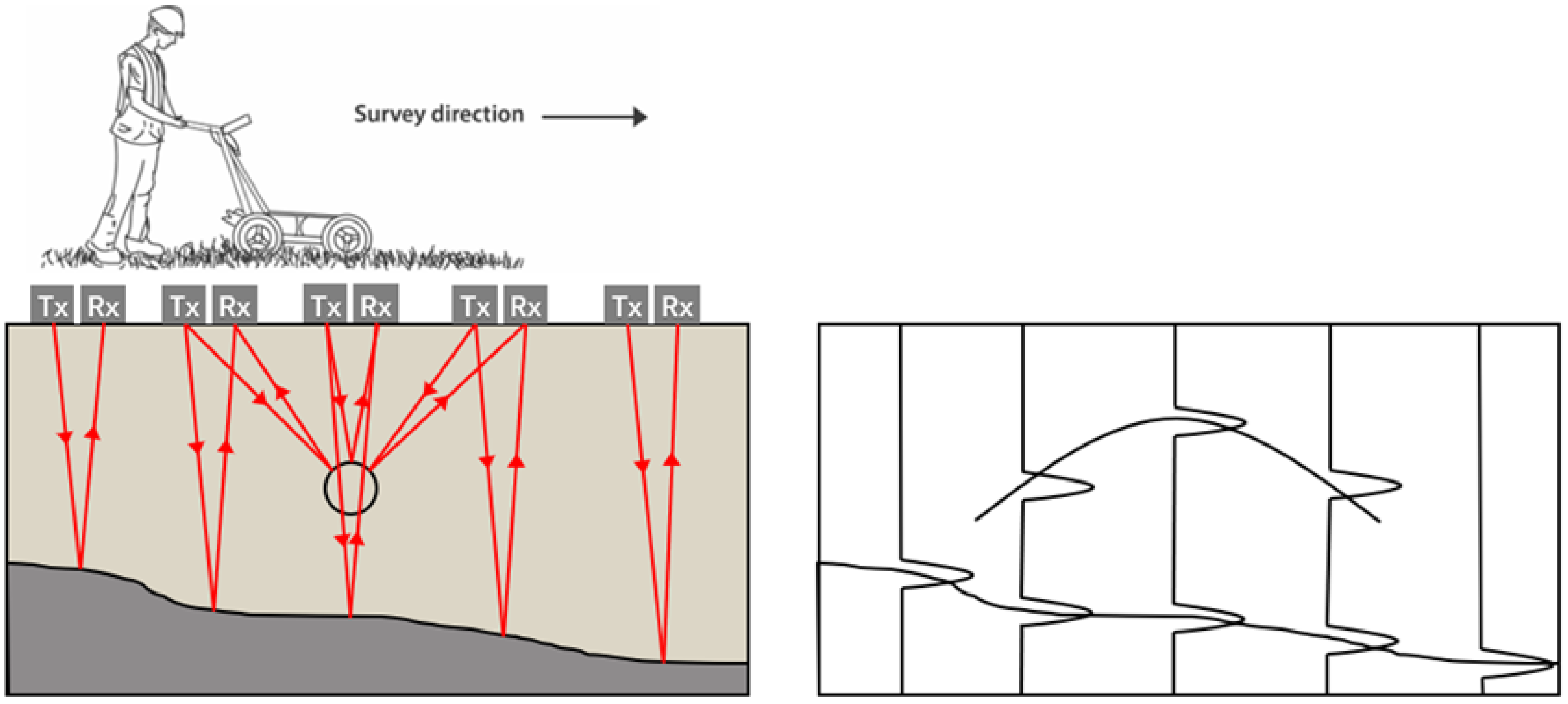
3. Basic Principle of GPR

During the operation of GPR, when the transmit and receive antennas are stationary, the received signal, called an A-scan, reflects the echo strength variance with underground depth. The amplitude, waveform and time delay of received echoes will change as they propagate and reflect through different media underground. As shown in Figure 1, When the GPR detection system moves, multiple A-scans are stacked horizontally to obtain GPR B-scan images. Horizontal resolution is the distance between two adjacent transmissions. Different subsurface targets show different characteristics in the B-scan images. For example, horizontal layer soil structure is characterized by the curves with shapes similar to interface, whereas cylindrical objects such as underground pipes are characterized by hyperbola.

The most widely used numerical simulation method for GPR signals and images is the finite difference time domain (FDTD) method [17,18]. It uses a finite difference equation to approximate the two curl equations in Maxwell’s equations, using the Yee grid to discretize the space and iterate through the time dimension. The most widely used simulation software is gprMax with FDTD as a kernel [19]. It is mainly written in Python 3, with performance-critical parts written in Cython and many functional features are designed and optimized specifically for the GPR domain. The simulation data in this paper are generated using gprMax software.

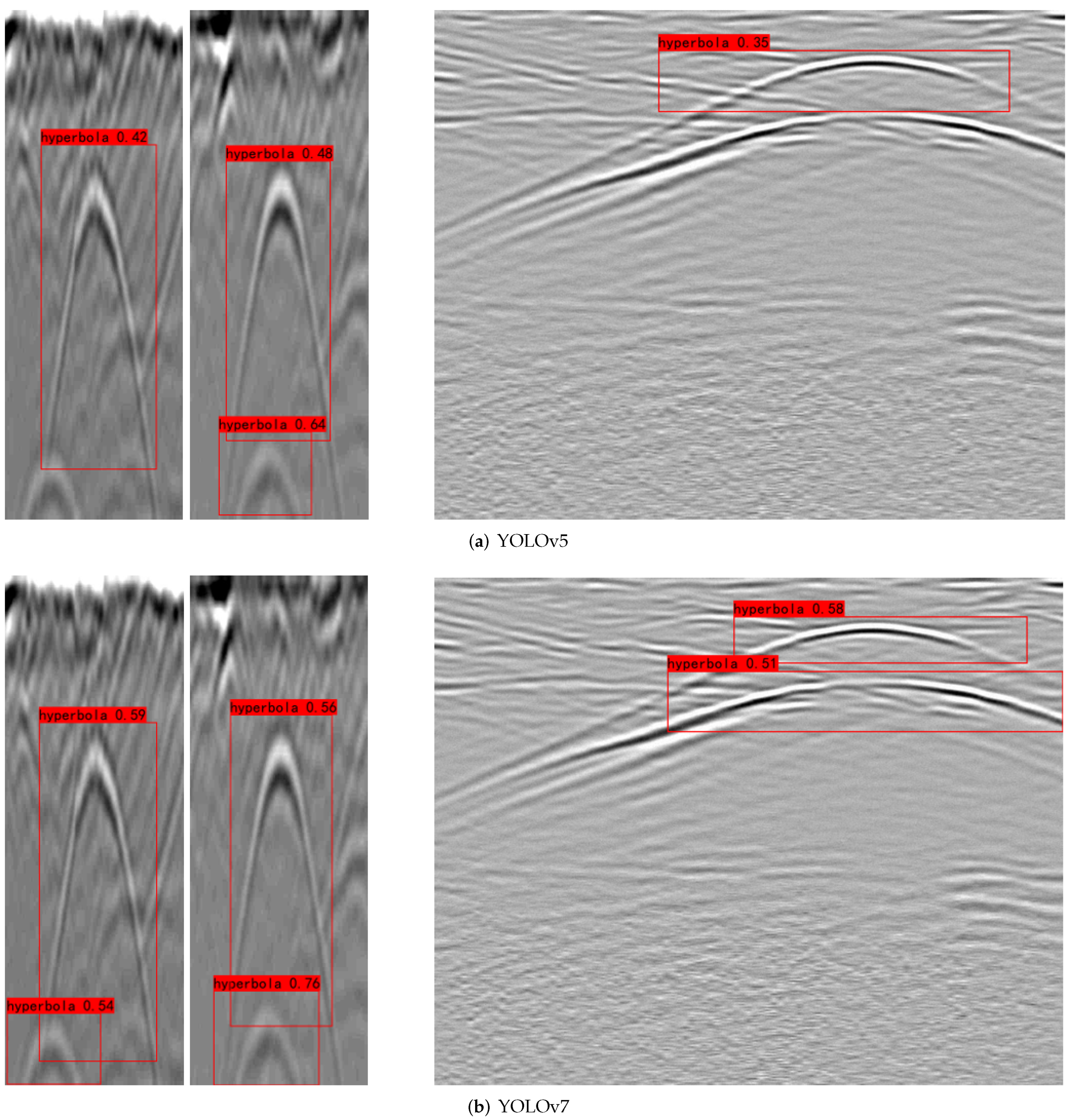
4. Detection of GPR Hyperbolic Features Based on YOLOv7

4.1. Data Preparation

This paper uses GPR images published on https://github.com/irenexychen/gpr-data-classifier (accessed on 15 April 2023) to create a dataset. The dataset contains a total of 209 images without target location information. After deleting the images without obvious hyperbolic features, the remaining images are divided into two categories, different strategies are adopted to deal with these two categories of data. The following operations on images are completed using functions in the transforms and imgaug libraries.

The first category consists of 69 greyscale images with a resolution of 500 × 350. The hyperbolic features in these images are weak, so the adjust contrast function is used in torchvision’s transforms library to adjust the contrast of the image to deepen the hyperbolic contours, as shown in Figure 2. Then the resize function is used to take each image stretched horizontally to a resolution of 500 × 1400 and vertically to a resolution of 1000 × 350 and the original and stretched images are flipped horizontally. The stretching of the horizontal resolution can simulate different dx, the stretching of the vertical resolution can simulate different dt and the horizontal flipping can simulate different detection directions. After processing, the number of first category images expanded to 414.

The second category consists of 88 blue-tinted B-scan images of variable resolution with axis information. We took only the central part of the data and converted it to grey scale, as shown in Figure 3.

A total of 502 images were obtained after the above processing and then randomly mirrored, the brightness was adjusted, Gaussian noise was added and all images were resized using the imgaug library, resulting in a total of 3012 images. They were divided into a training set and a validation set in the ratio 9:1 and sent to the network. The network uses the idea of migration learning, using initial weights pre-trained on the COCO dataset. This approach gives the network the ability to extract shallow features and can speed up model convergence and improve generalization on small datasets.

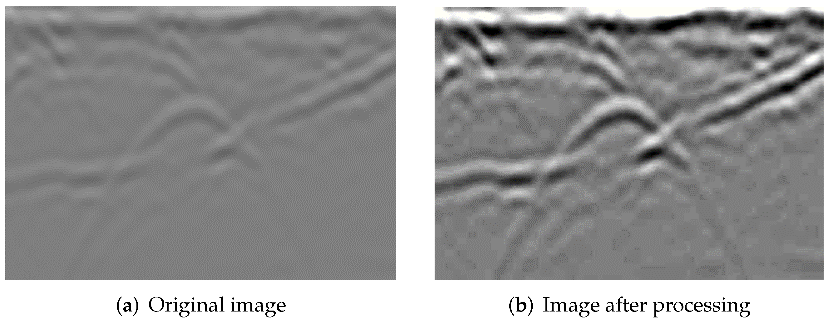
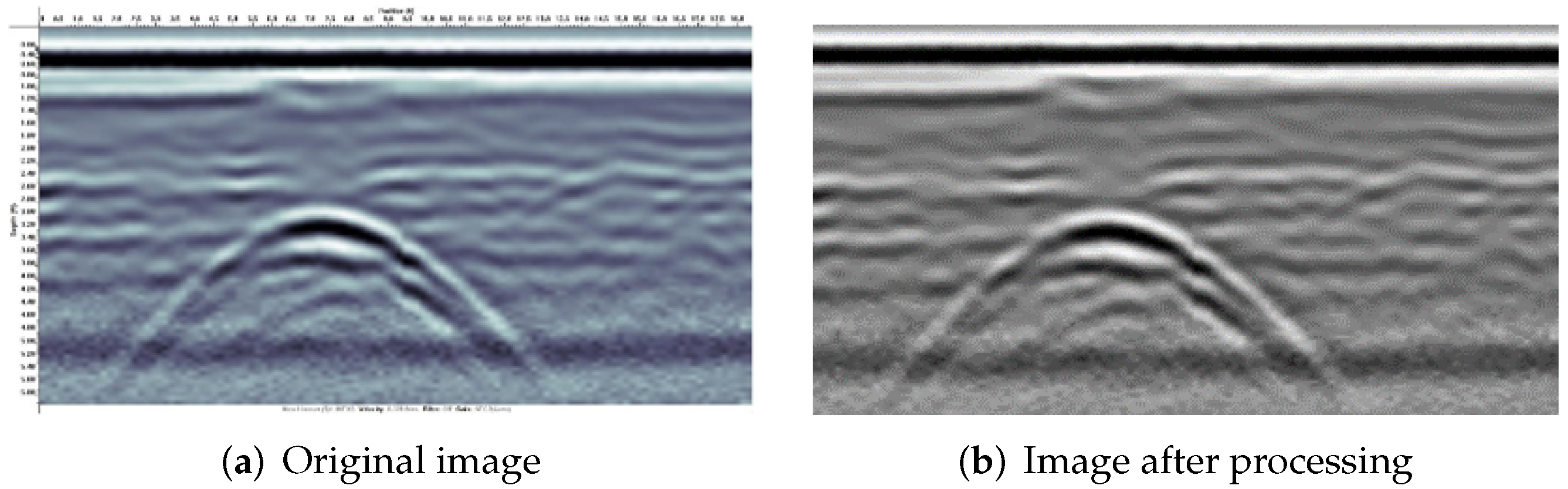
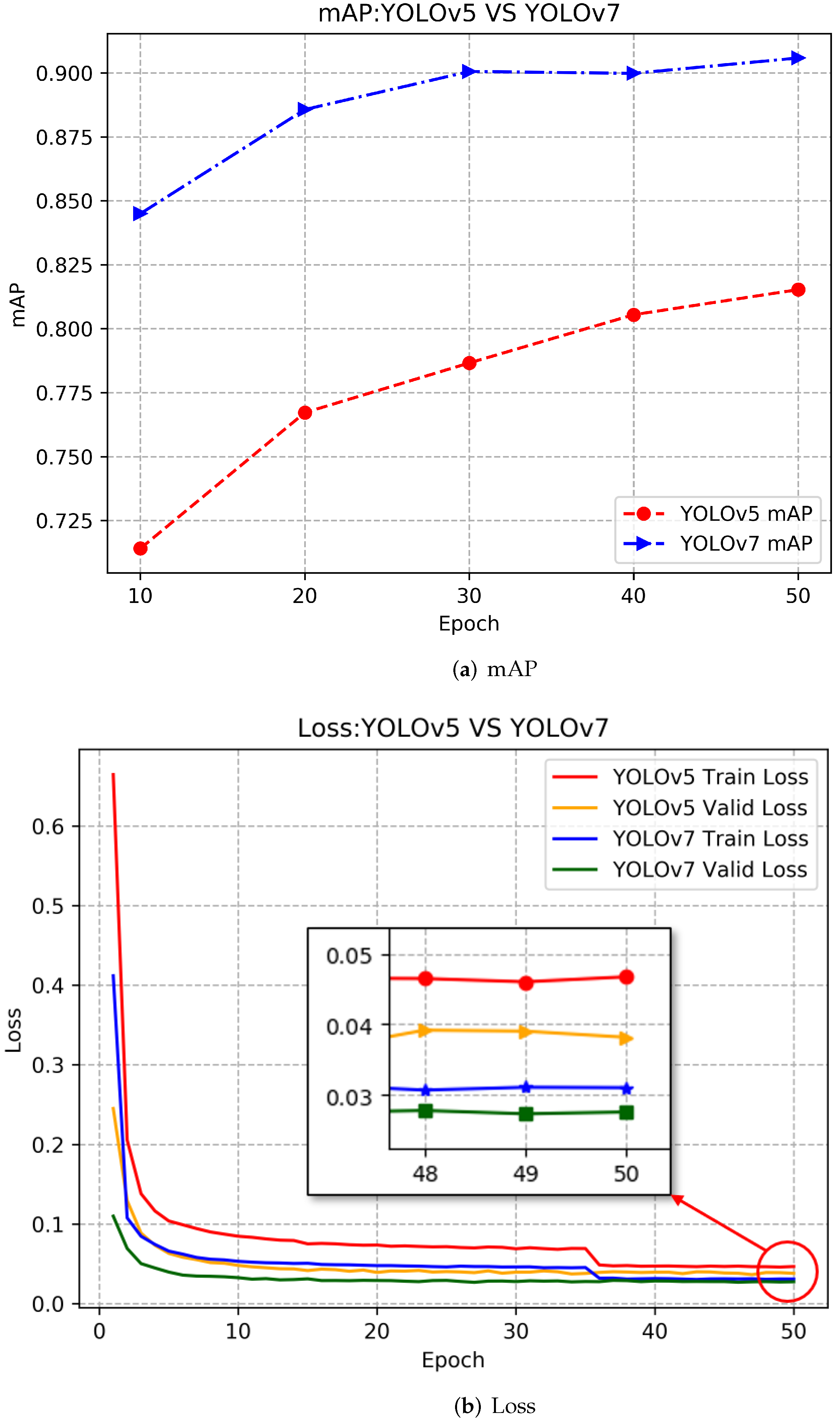
4.2. Comparison of Results

The YOLOv5 and YOLOv7 networks were trained on the same hardware. Both were trained for 50 epochs and the batch size was set to 8. Using the sgd optimizer, the momentum was set to 0.937 and the weight decay was set to $5\times {10}^{-4}$. The mAP was calculated every 10 epoch and the results are shown in Figure 4a. The change in loss during training is shown in Figure 4b.

The five mAP calculations for YOLOv5 were 0.71, 0.77, 0.79, 0.81 and 0.82; the five mAP calculations for YOLOv7 were 0.84, 0.89, 0.90, 0.90 and 0.91. As can be seen in Figure 4a, the accuracy of YOLOv7 was higher than that of YOLOv5 for each mAP. After training, the mAP of YOLOv5 is 81.53%, while that of YOLOv7 is 90.58% and the accuracy of YOLOv7 has an 11.1% improvement over YOLOv5. As can be seen in Figure 4b, YOLOv7 has lower train loss and valid loss compared to YOLOv5. Then comes the speed comparison, where YOLOv7 achieves an FPS of 22.1 for detection, compared to 18.7 for YOLOv5. YOLOv7 achieves a speed improvement of 18.2% over YOLOv5.

Figure 5 shows the results of detecting the same GPR images using YOLOv5 and YOLOv7. As can be seen from the images, the prediction results of YOLOv7 have the following advantages: 1. a higher confidence level for the same hyperbolic feature; 2. fewer missed hyperbolas.

5. Parameter Inversion of Pipeline Based on Key Point Annotation

In the previous section, the hyperbolic features in GPR B-scan images were detected using object detection techniques in deep learning. In this section, the constraint equations of hyperbolic features and underground pipeline parameters are further established based on the principles of GPR imaging and the quantitative inversion of pipeline parameters is achieved using curve fitting based on the gradient descent method. To solve these problems, a graphical user interface was developed to invert the depth and radius of the underground pipes by annotating the key points of the hyperbola and the time and distance sampling intervals of the GPR system. The method requires little image processing, just the key points in the hyperbola, reducing the calculations of the previous algorithms. It also uses an innovative two-stage fitting strategy based on the physical model of detection, which improves the curve-fitting effect.

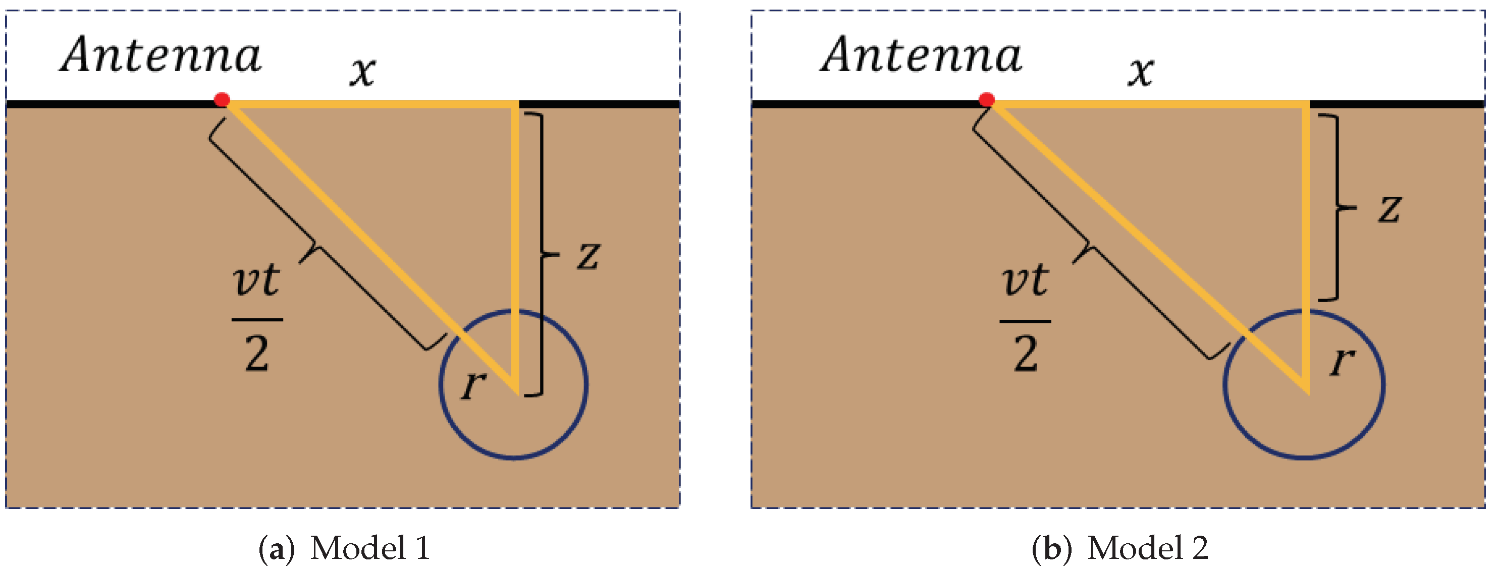
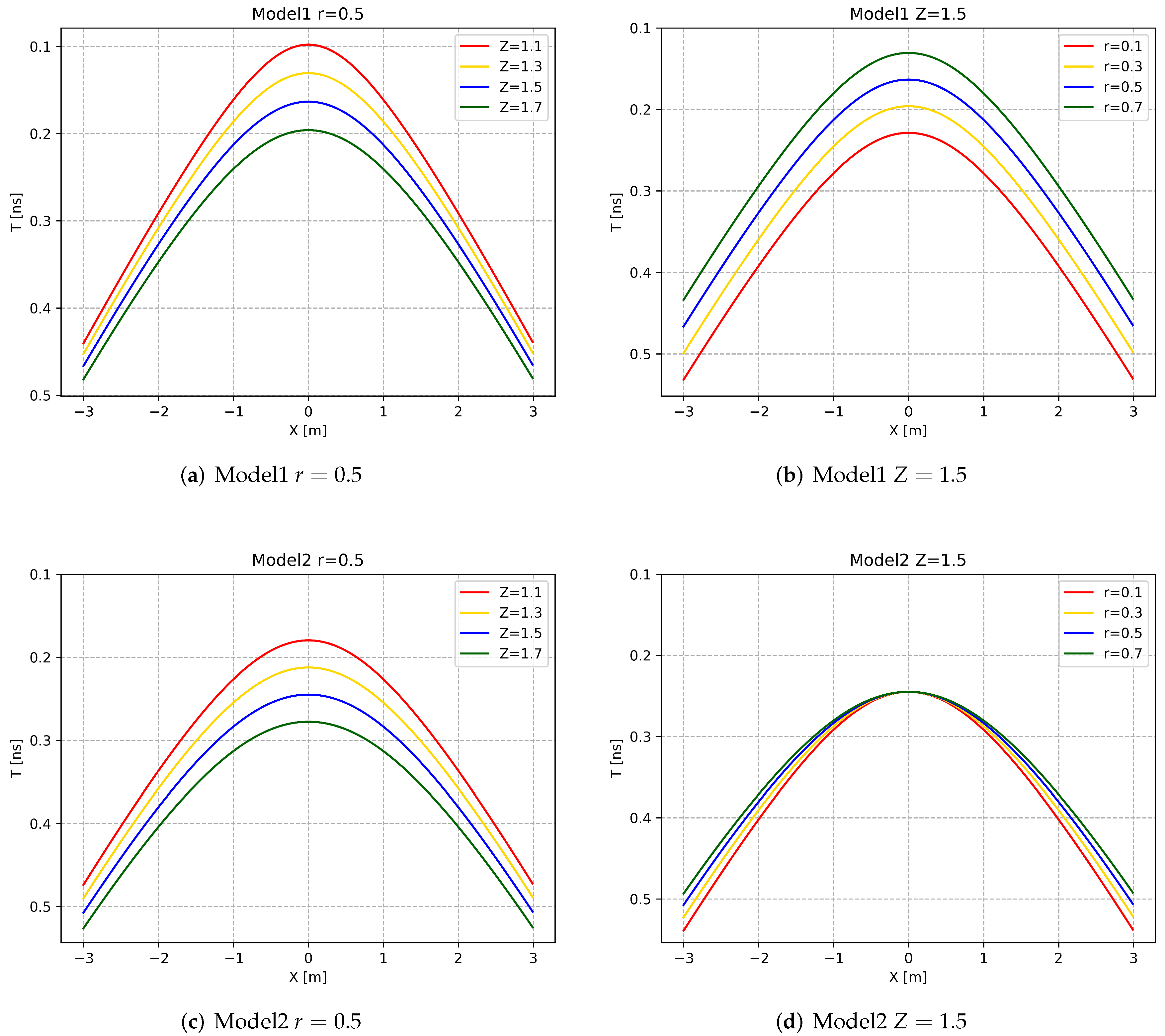
5.1. Physical Model of GPR Detection

The definition of the pipe’s depth in different detection models results in different constraint equations, which can change the way the parameters affect the shape of the hyperbola.

As shown in Figure 6, Model 1 defines depth as the distance from the surface to the center of the pipe and Model 2 defines depth as the distance from the surface to the upper tangent plane of the pipe. According to the geometric relationship of the golden triangle in Figure 6, the two-way propagation time t of the electromagnetic wave in the two models is shown in Equations (1) and (2), respectively.

$$t1=\frac{2(\sqrt{x^2+z^2}-r)}{v}$$

(1)

$$t2=\frac{2(\sqrt{x^2+{(z+r)}^2}-r)}{v}$$

(2)

Here x is the lateral distance between the antenna and the center of the pipe, z is the depth of the pipe, r is the radius of the pipe and v is the propagation velocity of the electromagnetic wave in the background medium.

From Figure 7, it can be seen that in Model 1, the changes in both depth and radius cause the upward and downward shifts of the hyperbola. When the depth gradually increases, the increase in the two-way propagation time causes the hyperbola to shift downward; when the radius gradually increases, the decrease in the two-way propagation time causes the hyperbola to shift upward because the center of the metal cylinder does not move. This makes the inversion process difficult because it is impossible to determine whether the depth or the radius should be adjusted for the same section of longitudinal displacement. In Model 2, however, the change in depth only moves the hyperbola up and down, while the change in radius only determines the angle of expansion of the hyperbola, which is advantageous for the subsequent parameter inversion. Therefore, the subsequent inversion process will use Model 2 as the physical model and Section 5.3 proposes an innovative two-stage curve fitting method based on the characteristics of Model 2.

All the above discussions are carried out while keeping the wave speed v constant. In fact, the wave speed v also causes the hyperbola to move up and down, as can be seen in Equations (1) and (2), where the change in v actually multiplies t by a factor. In order to be able to invert correctly, we assume that the wave velocity (or the relative permittivity of the medium) can be obtained by other measurement methods.

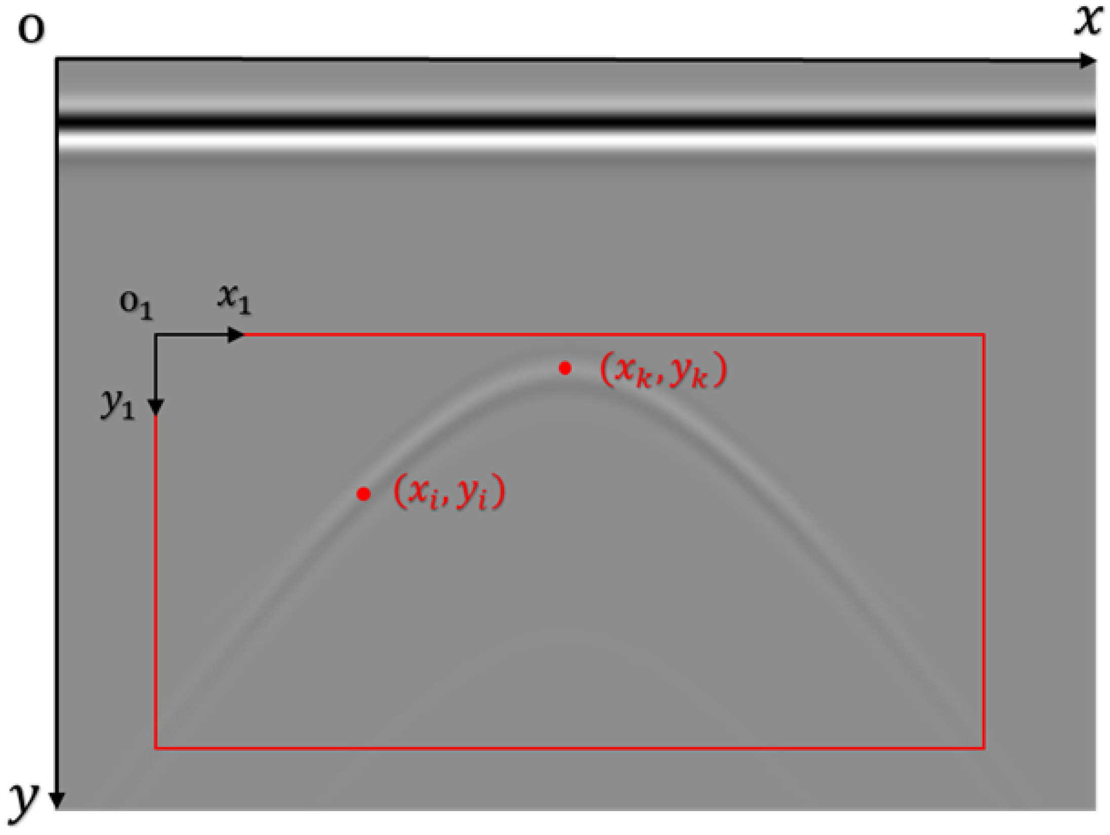
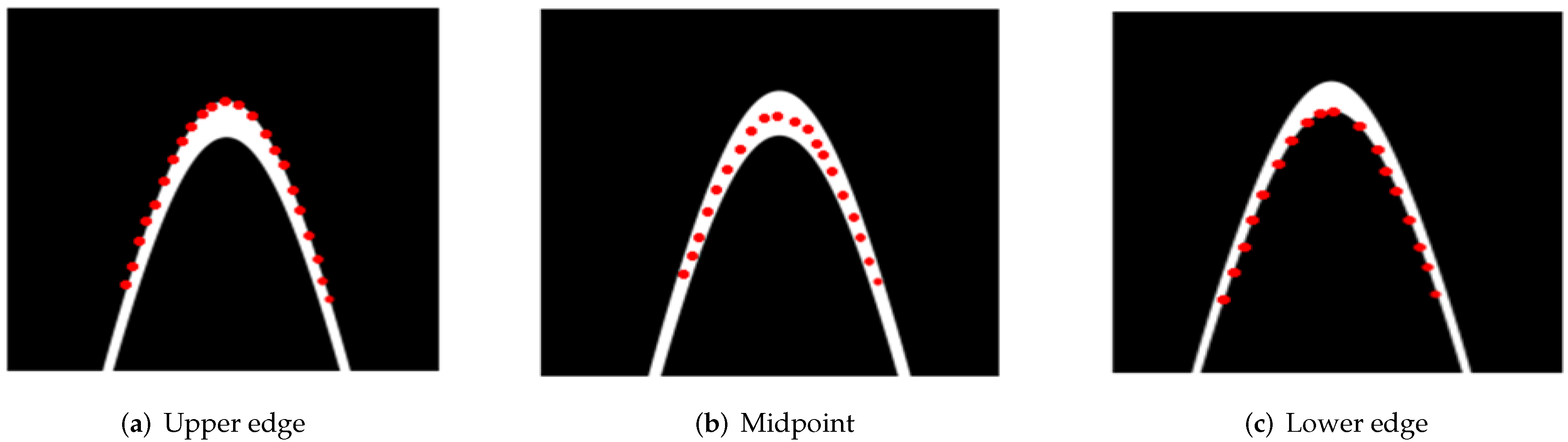
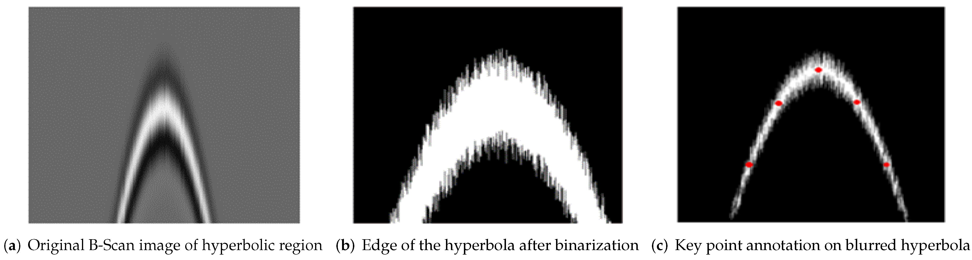
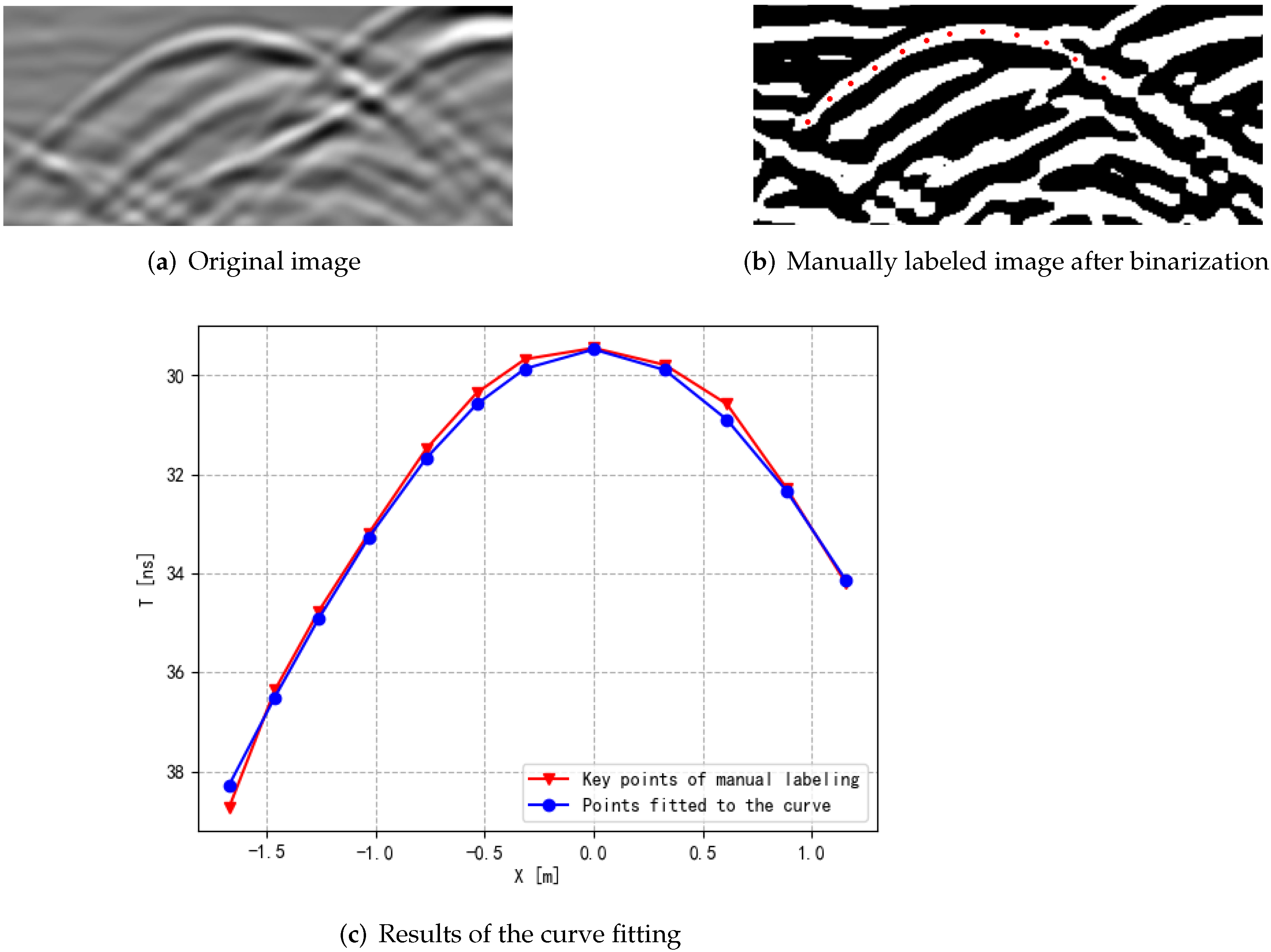
5.2. Coordinate Transformation of Key Points

Convert the pixel coordinates of key points to real physical coordinates. When using the mouse for key point annotation, the system records the coordinates of the pixel point of the mouse click position in the local B-Scan image. In order to compare with the detection model, it is necessary to map the pixel location of the key point to the real physical location. The specific steps are as follows.

1. As shown in Figure 8, a global coordinate system $xoy$ is established in the original B-Scan image and a local coordinate system $x_1{o}_1{y}_1$ (the part in the object detection box) is established in the local B-Scan image. Suppose the coordinates of a key point in the local coordinate system are $(x_i,y_i)$ and the coordinates of the local coordinate system origin $o_1$ in the global coordinate system are $(x_o,y_o)$, then the coordinates of the key point in the global coordinate system are $(x_i+x_o,y_i+y_o)$. Following the same method, we obtain the pixel coordinates of each key point in the original B-Scan image.

2. Find the key point with the smallest y-coordinate in 1, which corresponds to the vertex of the hyperbola and assume that the coordinates of this point are $(x_k,y_k)$. The difference between the transverse coordinates of the other key points and $x_k$ is calculated and multiplied by the transverse inter-tract distance of the GPR system to obtain the x of each key point in the detection model with $x_k$ as the origin.

3. According to the basic information of the scene, appropriate initial values are set for z and r. Assuming that the maximum depth of the scene is $Z_{max}$, the initial value of the depth $Z_0$ must not exceed $Z_{max}$ and the initial value of the radius $r_0$ must not exceed $Z_{max}/2$. The gradient descent method is used to update Z and r step by step.

5.3. Two-Stage Curve Fitting and Inversion of the Parameters

According to the model characteristics described in Section 5.1, this paper innovatively uses two-stage curve fitting and inversion parameters in the following steps.

1. First, the radius is kept constant and only the depth is inverted. The loss function used in this stage is the relative error between the vertices, as shown in Equation (3).

$$Loss1=\left|\frac{t_0-t_1}{t_0}\right|$$

(3)

Here $t_0$ is the propagation time corresponding to the labeled hyperbolic vertices and $t_1$ is the propagation time corresponding to the hyperbolic vertices calculated using the inversion parameters and the model.

2. The depth is kept constant and only the radius is inverted. The loss function used in this stage is the mean square error function, as shown in Equation (4).

$$Loss2=\frac{1}{n}\sum _{i=1}^n{(t_{0i}-t_{1i})}^2$$

(4)

Here $t_0$ is the two-way propagation time series obtained by transforming the labeled key points and $t_1$ is the two-way propagation time series calculated using the inversion parameters and Equation (1).

After starting the inversion, the code will continuously reduce the error between the t obtained from the key points and the t calculated by the formula according to the above strategy and the inversion results of the obtained parameters will be displayed in the GUI after the fitting is finished, as shown in part 5 in Figure 9.

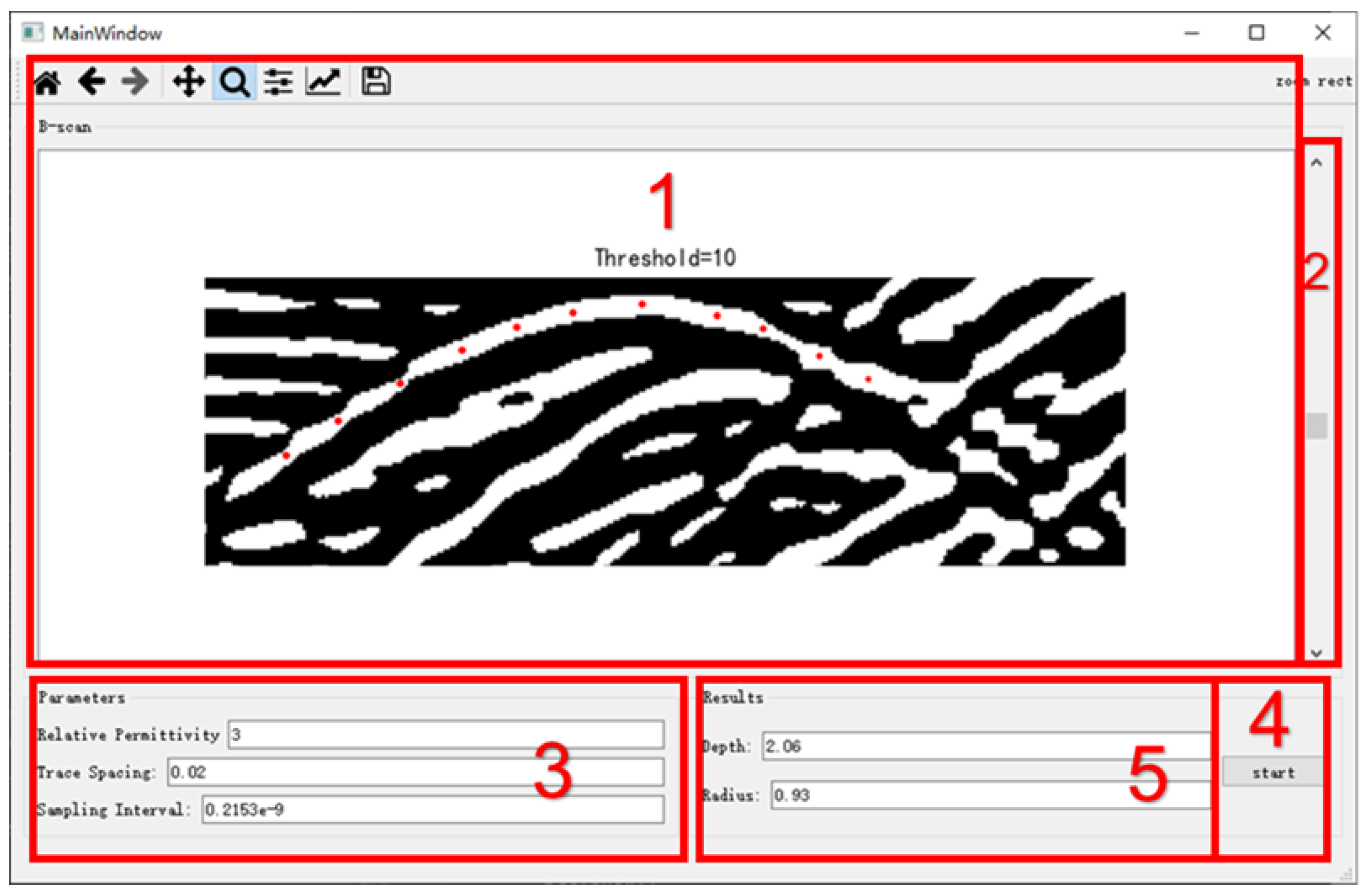
5.4. Introduction of the Graphical User Interface

The whole graphical user interface is shown in Figure 9, which is divided into five parts with the following specific functions.

1. Box 1—display and interaction of the GPR B-Scan signal. This part shows the local B-Scan image detected via the object detection module. The interaction functions include dragging, zooming, undoing, etc. Moreover, you can use the right mouse button to mark key points on the image and this window will also show the marked positions.

2. Box 2—threshold adjustment. Use the scroll bar to adjust the threshold size of the threshold segmentation, so that the hyperbolic outline can be displayed more clearly, to facilitate the marking of hyperbolic key points.

3. Box 3—radar basic parameters. Parameters include the relative dielectric constant of the subsurface medium, the sampling interval of the radar system and the distance between lateral channels.

4. Box 4—start button. After clicking the start button, the program will perform hyperbolic fitting and invert the target parameters based on the key point coordinates and the input radar parameters.

5. Box 5—result display. The results of the parameter fitting in step 4 will be displayed in this rectangular box.

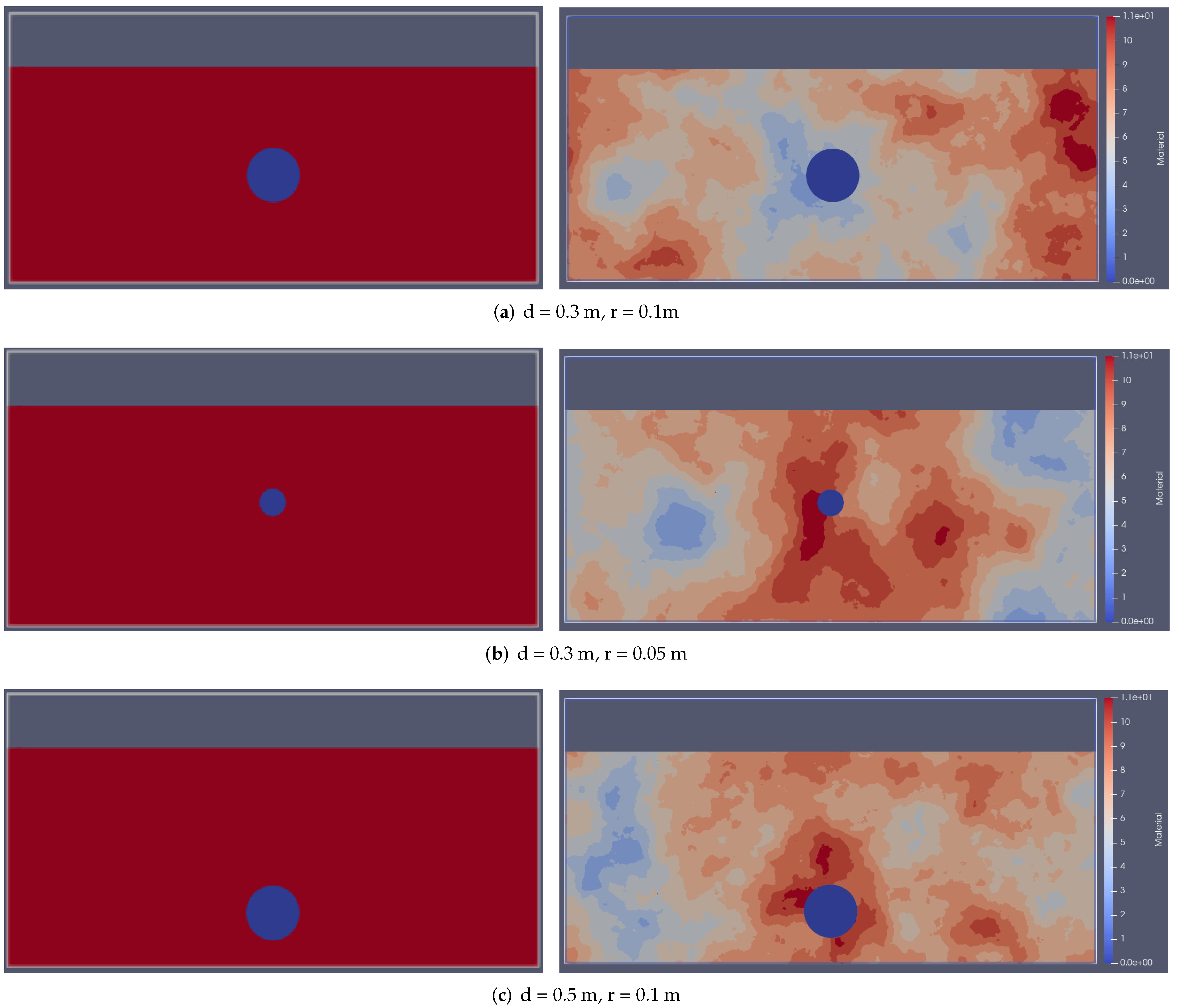
5.5. Performance Analysis with Synthetic Data

Two groups of six models with different background medium ${ϵ}_r$, embedding depth d and pipeline radius r, as shown in Figure 10, were simulated using the simulation software gprMax. The scene size of all the models is 2 m × 1 m; the spatial resolution is 0.001 m. The background of the left model is a homogeneous medium with relative permittivity ${ϵ}_r=6$. The background of the right model is a hybrid soil model proposed by Peplinski [20] with the average relative permittivity ${ϵ}_r=8.43$. There are three different depths and radiuses of PEC subsurface pipes buried in each scene: (a) d = 0.3 m and $\mathrm{r}=0.1$ m; (b) $\mathrm{d}=0.3$ m and $\mathrm{r}=0.05$ m; (c) $\mathrm{d}=0.5$ m and $\mathrm{r}=0.1$ m. The excitation source is a Ricker wave with center frequency $f_0=1$ GHz, the simulation time window of each A-scan echo is 15 ns. The transceiver antenna moves 1.9 m perpendicular to the direction of the pipe axis and a total of 1900 A-Scan data are detected to generate the B-scan images for postprocessing with the above algorithm. The in files for all six models are listed in Appendix A.

• Homogeneous medium model

The simulated B-Scan image of the homogeneous medium scene has clear hyperbolic features. Since the excitation source signal has a time width, the hyperbolic feature also has a width. The upper edge, midpoint and lower edge of the hyperbolic feature are used for the key point marker, as shown in Figure 11. The inversion results with the above method are shown in

Table 1. Inversion results of depth of homogeneous medium model.

Models	Labels	Before Correction	After Correction	Relative Error
a	Upper edge	0.3691
	Middle point	0.3803
	Lower edge	0.3908
b	Upper edge	0.3691	0.3	0%
	Middle point	0.3819	0.3016	0.50%
	Lower edge	0.39	0.2992	0.30%
c	Upper edge	0.5704	0.5013	2.60%
	Middle point	0.5803	0.5	0%
	Lower edge	0.5892	0.4984	0.30%

and

Table 2. Inversion results of radius of homogeneous medium model.

Models	Labels	Before Correction	After Correction	Relative Error
a	Upper edge	0.0599
	Middle point	0.0458
	Lower edge	0.0215
b	Upper edge	0.0057	0.0458	8.40%
	Middle point	−0.0031	0.0511	2.20%
	Lower edge	−0.0269	0.0516	3.20%
c	Upper edge	0.0682	0.1083	8.30%
	Middle point	0.0502	0.1044	4.40%
	Lower edge	0.0248	0.1033	3.30%

. When the midpoint of the hyperbolic curve is selected for key points, the inversed depths of all three models have a deviation of about 0.08 m from the true value and the deviation of the radius is about 0.05 m. The error of the burial depth is due to the fact that the time corresponding to the apex of the hyperbola contains the EM wave roundtrip time and the rise time taken of excitation source amplitude from 0 to the maximum. In general, the depth deviation is a constant when the excitation source is fixed. The radius error is related to the channel spacing. Therefore, the error of one model can be used to correct other models when the same radar system is used. The deviation of model (a) in Figure 10 is used to calibrate other models. After the correction, the relative error of the burial depth is only about 0.6% and the relative error of the radius is only about 4.4%. The absolute error of both burial depth and radius is millimeter level. This result verifies the feasibility of the method in this paper.

The inversion value of radius in Table 2 shows negative numbers. The analysis of detection models demonstrates that the expansion angle of the hyperbola changes monotonically as the radius goes from negative to positive. This indicates that the negative number is only a numerical solution derived from the shape of the hyperbola and does not represent the real physical result and the correct positive result can be obtained after correcting the radius.

•

Non-homogeneous medium model

As shown in Figure 12, the hyperbolic features in the B-Scan image are blurred and have rough edges, making it difficult to identify the upper and lower edges of the hyperbolic. Therefore, only the midpoint of the hyperbolic feature is used for inversion. The inversion results are shown in

Table 3. Inversion results of depth of non-homogeneous medium model.

Models	Before Correction	After Correction	Relative Error
a	0.4389	/
b	0.4389	0.3	0%
c	0.6869	0.548	9.60%

and

Table 4. Inversion results of radius of non-homogeneous medium model.

Models	Before Correction	After Correction	Relative Error
a	−0.0939	/
b	−0.1354	0.0585	17%
c	−0.0799	0.1140	14%

. After correction via the above method, the relative error of the depth is 4.8% and the relative error of the radius is about 15%. The non-homogeneous medium causes the vertex and midpoint of the hyperbolic feature to be more difficult to identify, so the relative errors of both the depth and radius inversion results are increased.

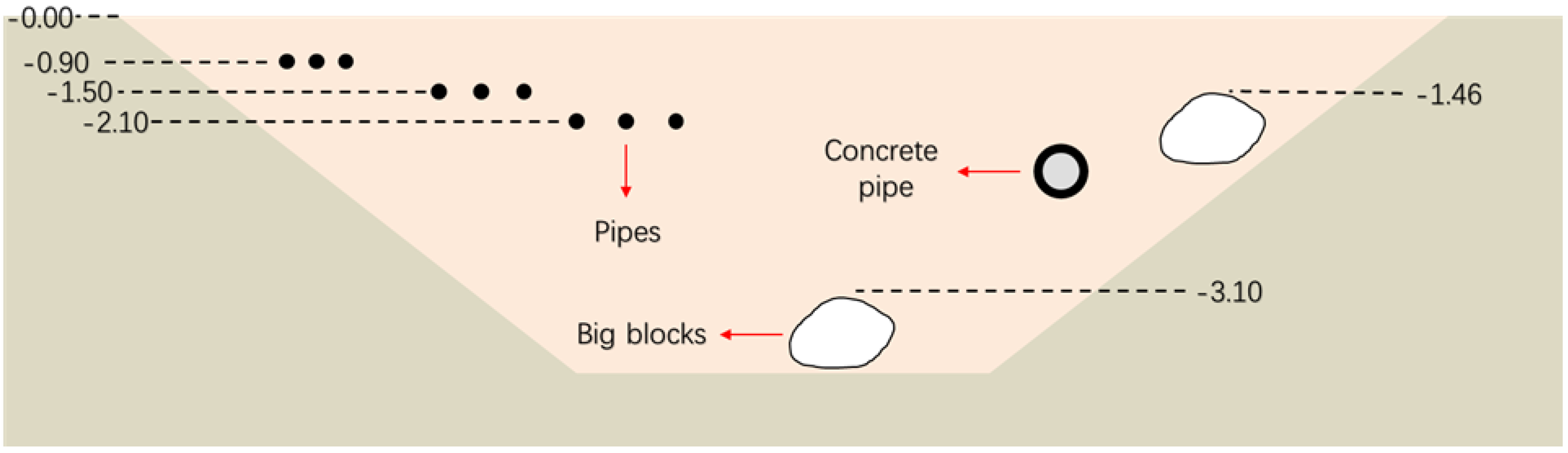
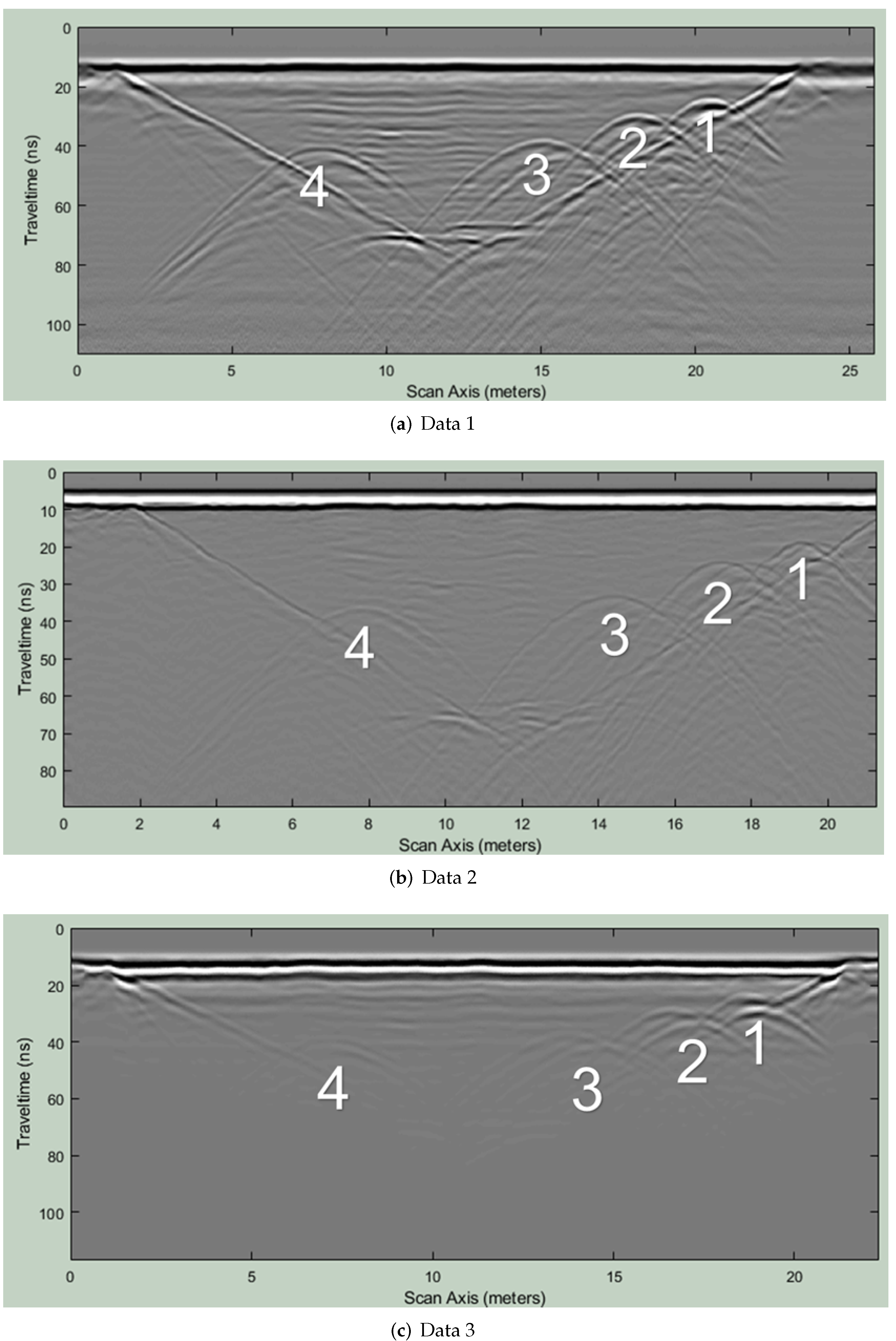
5.6. Performance Analysis with Measured Data

The measured data used in this paper are from the TU1208 radar open database of the IFTTAR geophysical test site [21], which reproduces common objects and obstacles in the urban subsurface in a fully controlled environment. The test site is a 30 m long, 5 m wide, laterally inclined pit with a useful area of approximately 4 m depth. The pit is divided into five sections filled with different materials, such as silt, limestone and gneiss and separated by vertical interfaces. The test site also buried a number of typical targets that may be encountered during trenchless work, such as pipes, cables, various sizes of stone and masonry. The data set consists of 67 records along 11 survey lines that crossed the test site laterally using three pulsed radar systems. We finally selected three measurement records of the gneiss area with grain size 14–20 mm for inversion. The GSSI radar system with 200 MHz antenna and 400 MHz and the MALA system with 250 MHz are used to collect data. The scene setup of this gneiss area is shown in Figure 13. The relative dielectric constant of the subsurface medium is estimated to be ${ϵ}_r=3$. On the left, nine pipes are buried in three different layers of 0.9 m, 1.5 m and 2.1 m. Each layer has three pipes with different materials. They are an empty steel pipe, a PVC pipe filled with water and an empty PVC pipe from left to right. Due to the different materials, the hyperbolic signals generated by the three pipes will be slightly different. The steel pipe produces one hyperbola. The water-filled PVC pipe produces a first hyperbola from the top side of the pipe and a continuous hyperbola due to the reflection from its bottom (the amplitude is greater than the echo of the first hyperbola). The empty PVC pipe also produces reflections from its top side and bottom. Because the propagation velocity of electromagnetic wave in the air is higher than that in the water, the continuous echo is clearer than that of the empty PVC pipe. Three pipes of each layer are close to each other and the hyperbolic signals will overlap with each other. Therefore, in the subsequent processing, we only analyze the most obvious hyperbolic curve in each layer, labeled as No.1, 2 and 3 from top to bottom. There is also a concrete pipe with a diameter of 500 mm buried on the right side of the scene and the corresponding hyperbolic feature is labeled as No.4. Since the pipe diameter is about 8 to 10 cm, which is much smaller than radar wavelength, it is difficult to invert the radius of the pipe from the shape of the hyperbola. In the following, we only invert the depth of the pipe.

The basic parameters of the measured data are shown in

Table 5. Parameters of the measured data.

	GPR System	Antenna Frequency	Measuring Line Length	Channel Spacing	Number of A-Scan	Sampling Time Interval	Sampling Points
Data1	GSSI	200 MHz	25.8 m	0.02 m	1291	0.2153 ns	512
Data2	GSSI	400 MHz	21.27 m	0.03333 m	639	0.1761 ns	510
Data3	MALA	250 MHz	22.32 m	0.03033 m	737	0.2821 ns	415

.

Data 1 were detected via the GSSI system with 200 MHz antenna for 25.8 m; a total of 1291 A-Scan signals were collected. The lateral distance between each A-Scan signal was 0.02 m and the sampling time interval was 0.2153 ns. There were 512 sampling points for each A-Scan. The original data are shown in Figure 14a.

Data 2 were detected via the GSSI system with 400 MHz antenna for 21.27 m; a total of 639 A-Scan signals were collected. The lateral distance between each A-Scan signal was 0.03333 m and the sampling time interval was 0.1761 ns. There were 510 sampling points for each A-Scan. The original data are shown in Figure 14b.

Data 3 were detected via the MALA system with 250 MHz antenna for 22.32 m; a total of 737 A-Scan signals were collected. The lateral distance between each A-Scan signal was 0.03033 m and the sampling time interval was 0.2821 ns. There were 415 sampling points for each A-Scan. The original data are shown in Figure 14c.

Taking hyperbola #2 in Data 1 as an example, Figure 15a–c show the original image, the manually labeled image after binarization and the results of the curve fitting.

The three groups of measured data were processed using the above algorithm and the inversed depths of hyperbola 1 were used to correct hyperbolas 2, 3 and 4. The depth corrections for the three data were −1.21 m, −0.74 m and −1.05 m and the corrected results are shown in the

Table 6. Depth inversion results of the measured data.

	No. 1 Hyperbola		No. 2 Hyperbola			No. 3 Hyperbola			No. 4 Hyperbola
	Before	After	Before	After	Relative Error	Before	After	Relative Error	Before	After
Data1	2.11	/	2.54	1.33	11.30%	3.28	2.07	1.40%	3.54	2.34
Data2	1.64		2.08	1.34	10.70%	2.87	2.13	1.40%	3.11	2.37
Data3	1.95		2.43	1.38	8.00%	3.16	2.11	0.50%	3.41	2.36

.

After correction, the average absolute error of the inversion results of the depth of hyperbolic No. 2 is 0.15 m and the average relative error is 10.0%; the average absolute error of the inversion results of the depth of hyperbolic No. 3 is 0.02 m and the average relative error is 1.1%; the concrete pipe corresponding to hyperbolic No. 4 does not give the true value of the depth, but all three inversion results are very close, with the average value of 2.36 m, coincided with the burial situation, located below the third layer of pipes, and the variance was only 0.00017.

6. Conclusions

This paper proposes a modular detection and quantitative inversion method for the hyperbolic features in GPR B-Scan images. The entire method is implemented in two steps.

The first step of the method uses object detection in deep learning to automatically detect hyperbolic features in GPR B-Scan images. This paper verifies the feasibility of this step using YOLOv7 as an example and compares it with YOLOv5. Using the same hardware and data set, YOLOv7 achieves an 11.1% improvement in detection accuracy and an 18.2% improvement in speed compared to the YOLOv5.

For the second step of the method, a GUI was developed to facilitate manual annotation of key points. Through the analysis of different detection models, the model using the distance from the ground surface to the upper tangent plane of the pipe as the depth was selected and a two-stage curve fitting method was proposed according to the characteristics of this model. The method was validated on synthetic data in homogeneous media, synthetic data in non-homogeneous media and measured data. The relative errors for the depth and radius of the synthetic data in homogeneous media are 0.6% and 4.4%, respectively, and 4.8% and 15% in non-homogeneous media. The relative error of the depth inversion of the measured data TU1208 is less than 10%.The results show that the method can effectively invert the depth and radius of underground pipelines and reduce the difficulty of GPR data interpretation.

Due to the relative independence between the two steps, the modularity of the method is reflected in the fact that the first step can be easily replaced by a more accurate and faster object detection network in the future. This allows the method to update its own efficiency and accuracy in real time, taking advantage of the rapid advances in object detection technology. The detection model in the second step can be adjusted according to the actual situation, such as considering the spacing of the transceiver antenna, the distance from the ground, refraction, etc., which helps to further improve the accuracy.

References

1. Travassos, X.L.; Avila, S.L.; Ida, N. Artificial neural networks and machine learning techniques applied to ground penetrating radar: A review. Appl. Comput. Inform. 2021, 17, 296–308. [Google Scholar] [CrossRef]
2. Pham, M.T.; Lefèvre, S. Buried object detection from B-scan ground penetrating radar data using Faster-RCNN. In Proceedings of the IGARSS 2018-02018 IEEE International Geoscience and Remote SENSING Symposium, Valencia, Spain, 22–27 July 2018; pp. 6804–6807. [Google Scholar]
3. Hou, F.; Lei, W.; Li, S.; Xi, J.; Xu, M.; Luo, J. Improved Mask R-CNN with distance guided intersection over union for GPR signature detection and segmentation. Autom. Constr. 2021, 121, 103414. [Google Scholar] [CrossRef]
4. Li, Y.; Zhao, Z.; Luo, Y.; Qiu, Z. Real-time pattern-recognition of GPR images with YOLO v3 implemented by tensorflow. Sensors 2020, 20, 6476. [Google Scholar] [CrossRef] [PubMed]
5. Li, S.; Gu, X.; Xu, X.; Xu, D.; Zhang, T.; Liu, Z.; Dong, Q. Detection of concealed cracks from ground penetrating radar images based on deep learning algorithm. Constr. Build. Mater. 2021, 273, 121949. [Google Scholar] [CrossRef]
6. Liu, Z.; Wu, W.; Gu, X.; Li, S.; Wang, L.; Zhang, T. Application of combining YOLO models and 3D GPR images in road detection and maintenance. Remote Sens. 2021, 13, 1081. [Google Scholar] [CrossRef]
7. Xiang, Z.; Rashidi, A.; Ou, G. An improved convolutional neural network system for automatically detecting rebar in GPR data. In Computing in Civil Engineering 2019: Data, Sensing and Analytics; American Society of Civil Engineers: Reston, VA, USA, 2019; pp. 422–429. [Google Scholar]
8. Dou, Q.; Wei, L.; Magee, D.R.; Cohn, A.G. Real-time hyperbola recognition and fitting in GPR data. IEEE Trans. Geosci. Remote. Sens. 2016, 55, 51–62. [Google Scholar] [CrossRef]
9. Zhou, X.; Chen, H.; Li, J. An automatic GPR B-scan image interpreting model. IEEE Trans. Geosci. Remote. Sens. 2018, 56, 3398–3412. [Google Scholar] [CrossRef]
10. Lei, W.; Hou, F.; Xi, J.; Tan, Q.; Xu, M.; Jiang, X.; Liu, G.; Gu, Q. Automatic hyperbola detection and fitting in GPR B-scan image. Autom. Constr. 2019, 106, 102839. [Google Scholar] [CrossRef]
11. Youn, H.S.; Chen, C.C. Automatic GPR target detection and clutter reduction using neural network. In Proceedings of the Ninth International Conference on Ground Penetrating Radar, Santa Barbara, CA, USA, 29 April–2 May 2002; Volume 4758, pp. 579–582. [Google Scholar]
12. Xie, X.; Qin, H.; Yu, C.; Liu, L. An automatic recognition algorithm for GPR images of RC structure voids. J. Appl. Geophys. 2013, 99, 125–134. [Google Scholar] [CrossRef]
13. Ristić, A.; Bugarinović, Ž.; Vrtunski, M.; Govedarica, M. Point coordinates extraction from localized hyperbolic reflections in GPR data. J. Appl. Geophys. 2017, 144, 1–17. [Google Scholar] [CrossRef]
14. Mertens, L.; Persico, R.; Matera, L.; Lambot, S. Automated detection of reflection hyperbolas in complex GPR images with no a priori knowledge on the medium. IEEE Trans. Geosci. Remote. Sens. 2015, 54, 580–596. [Google Scholar] [CrossRef]
15. Feng, D.S.; Yang, Z.L. Automatic recognition of ground penetrating radar image of tunnel lining structure based on deep learning. Prog. Geophys. 2020, 35, 1552–1556. [Google Scholar]
16. Wang, C.Y.; Bochkovskiy, A.; Liao, H.Y.M. YOLOv7: Trainable bag-of-freebies sets new state-of-the-art for real-time object detectors. arXiv 2022, arXiv:2207.02696. [Google Scholar]
17. Yee, K. Numerical solution of initial boundary value problems involving Maxwell’s equations in isotropic media. IEEE Trans. Antennas Propag. 1966, 14, 302–307. [Google Scholar]
18. Hu, H.; Ye, H.; Jin, Y.Q. Fast calculation of scattering in planar uniaxial anisotropic multilayers. IEEE Access 2019, 7, 185941–185950. [Google Scholar] [CrossRef]
19. Warren, C.; Giannopoulos, A.; Giannakis, I. gprMax: Open source software to simulate electromagnetic wave propagation for Ground Penetrating Radar. Comput. Phys. Commun. 2016, 209, 163–170. [Google Scholar] [CrossRef]
20. Peplinski, N.R.; Ulaby, F.T.; Dobson, M.C. Dielectric properties of soils in the 0.3–1.3-GHz range. IEEE Trans. Geosci. Remote Sens. 1995, 33, 803–807. [Google Scholar] [CrossRef]
21. Dérobert, X.; Pajewski, L. TU1208 open database of radargrams: The dataset of the IFSTTAR geophysical test site. Remote Sens. 2018, 10, 530. [Google Scholar] [CrossRef]
Figure 1. Basic principle of GPR.
Remotesensing 15 02114 g001
Figure 2. Processing of the first category.
Remotesensing 15 02114 g002
Figure 3. Processing of the second category.
Remotesensing 15 02114 g003
Figure 4. mAP and loss of YOLOv5 and YOLOv7.
Remotesensing 15 02114 g004
Figure 5. Prediction results.
Remotesensing 15 02114 g005
Figure 6. Physical model with different definition of depth.
Remotesensing 15 02114 g006
Figure 7. The way parameters affect the shape of the hyperbola in different physical model.
Remotesensing 15 02114 g007
Figure 8. Coordinate transformation of key points.
Remotesensing 15 02114 g008
Figure 9. Graphical user interface.
Remotesensing 15 02114 g009
Figure 10. Model schematic.
Remotesensing 15 02114 g010
Figure 11. Three different labeling methods.
Remotesensing 15 02114 g011
Figure 12. Synthetic data of non-homogeneous medium model.
Remotesensing 15 02114 g012
Figure 13. Scene setup of gneiss area.
Remotesensing 15 02114 g013
Figure 14. Original data.
Remotesensing 15 02114 g014
Figure 15. Manual labeling and curve fitting results.
Remotesensing 15 02114 g015