
SAR Image Quality Assessment: From Sample-Wise to Class-Wise

Abstract
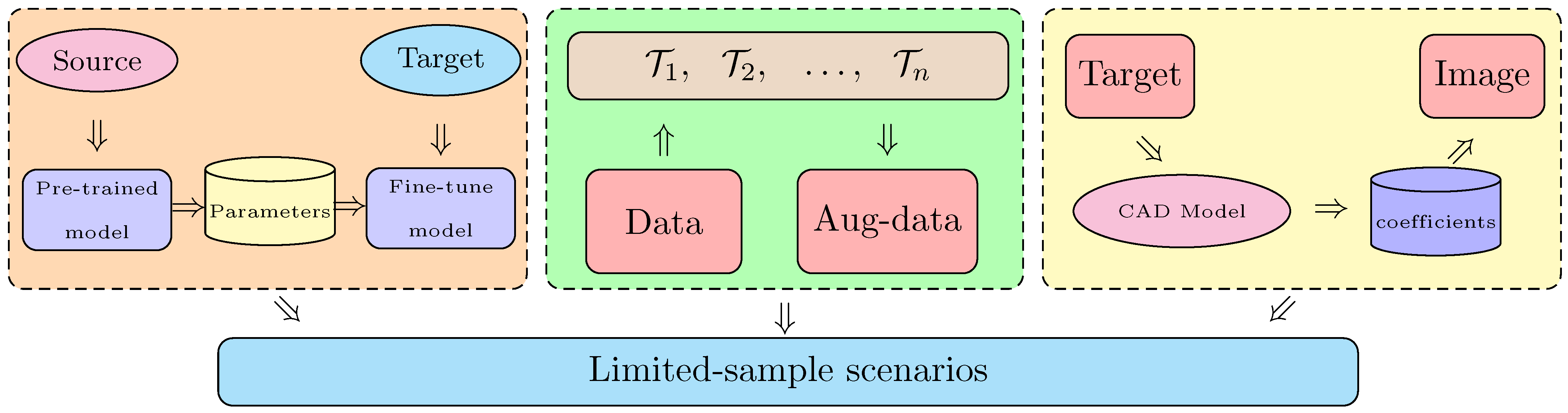
:1. Introduction
- (a)
- The sample-wise assessment is used to evaluate whether the relative intensity of the speckle noise of the SAR image and the target backscattering coefficients are well simulated.
- (b)
- The class-wise assessment is designed to compare the application capability of the simulated images in holistic.

2. The Related Works
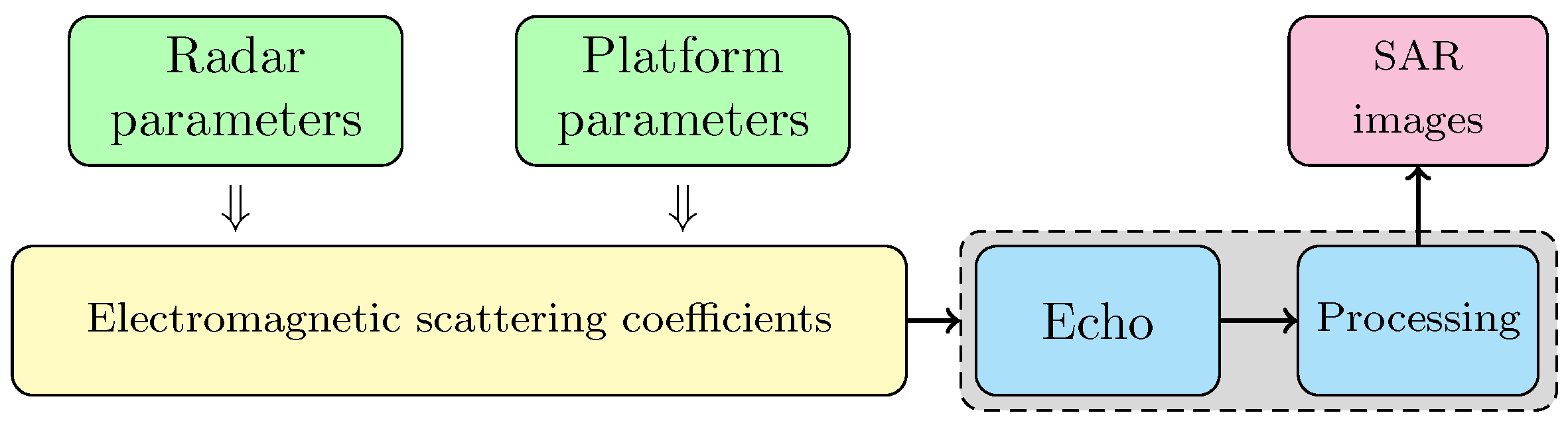
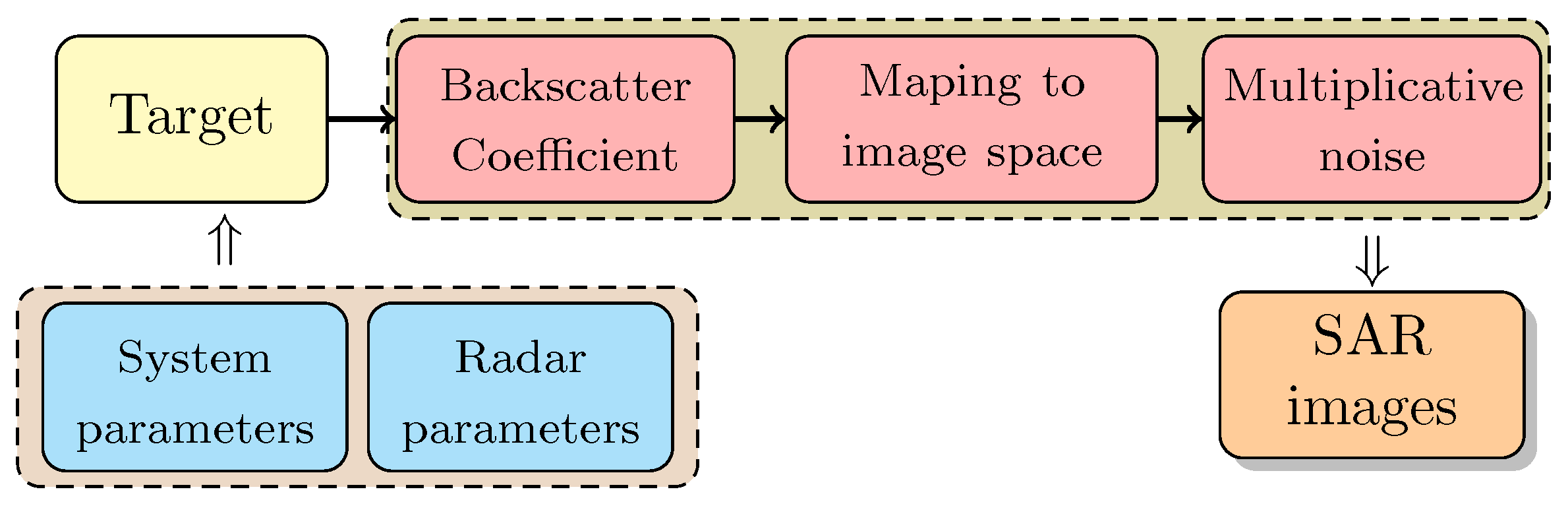
2.1. Simulation via Electromagnetic Computational Tools
2.1.1. SAR Image Simulation Based on Echo Signal
2.1.2. Feature-Based SAR Image Simulation
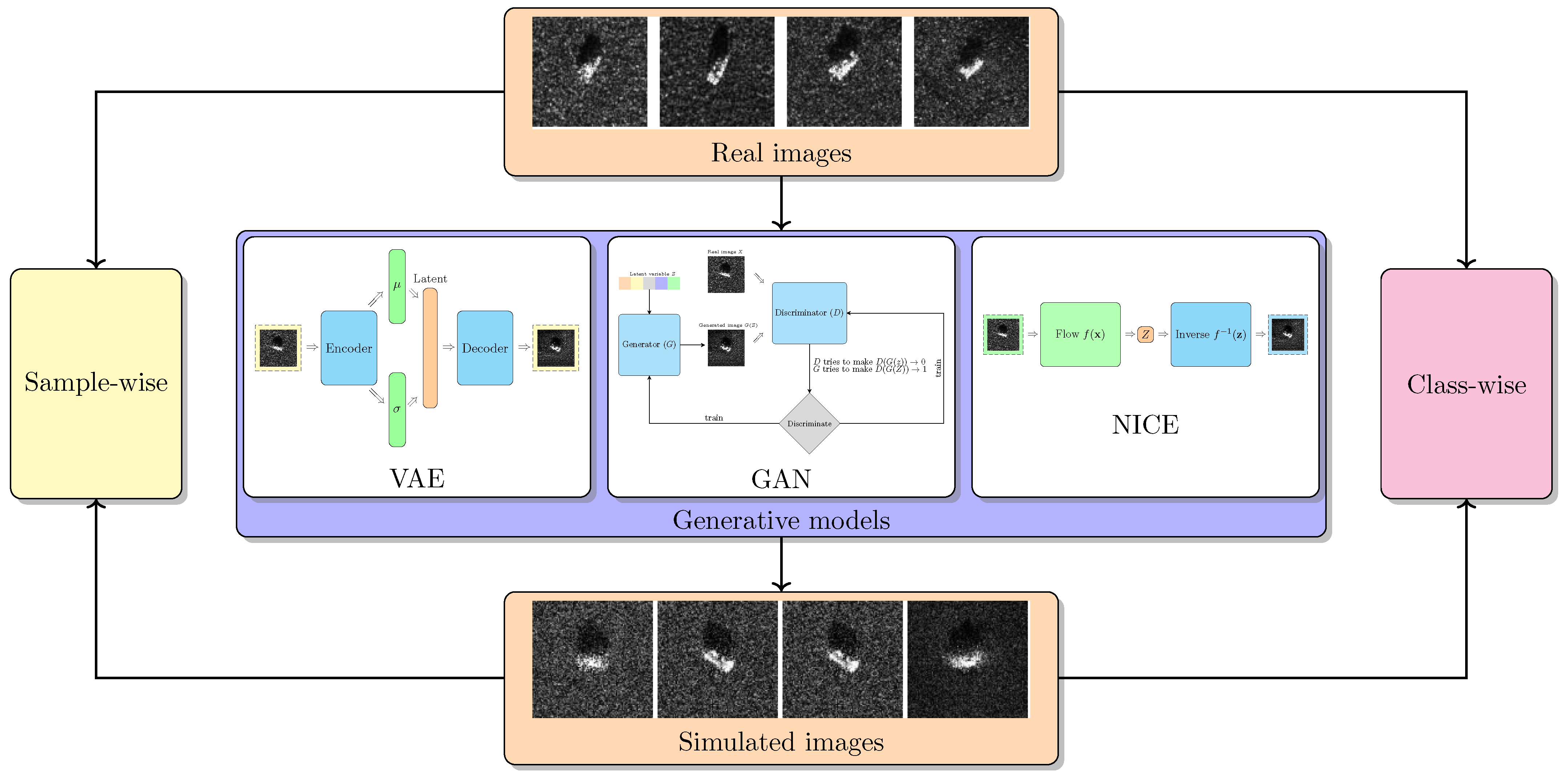
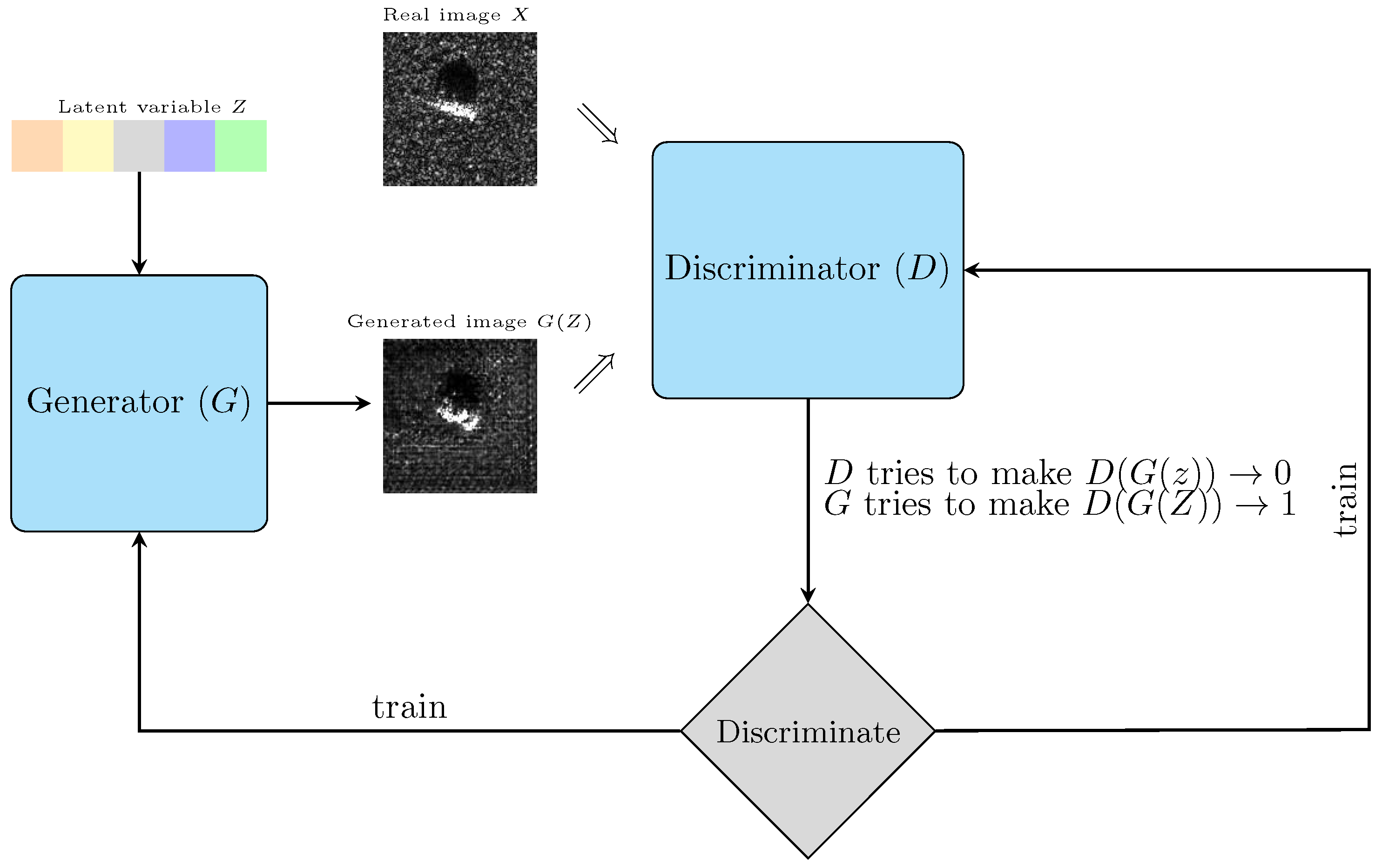
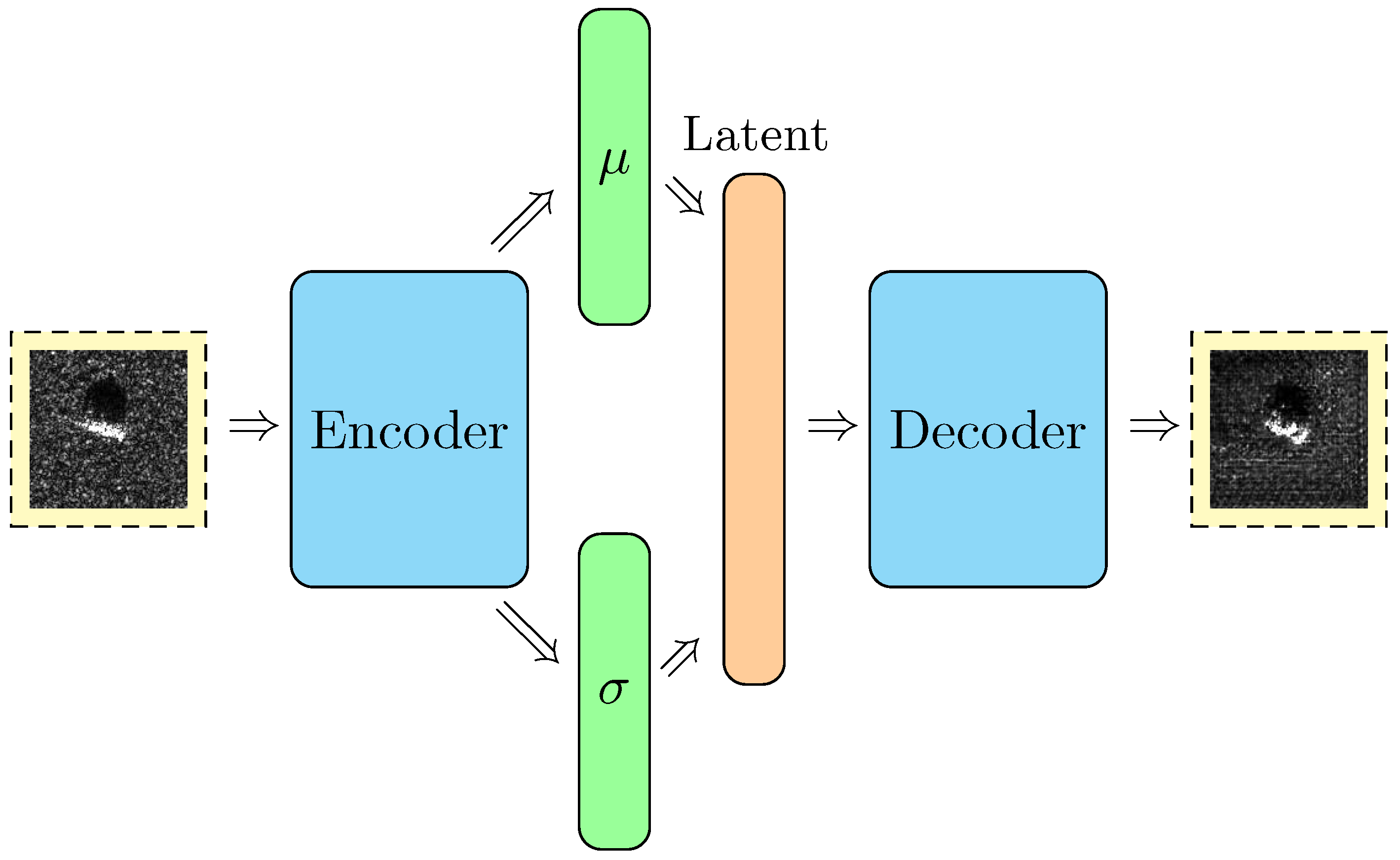
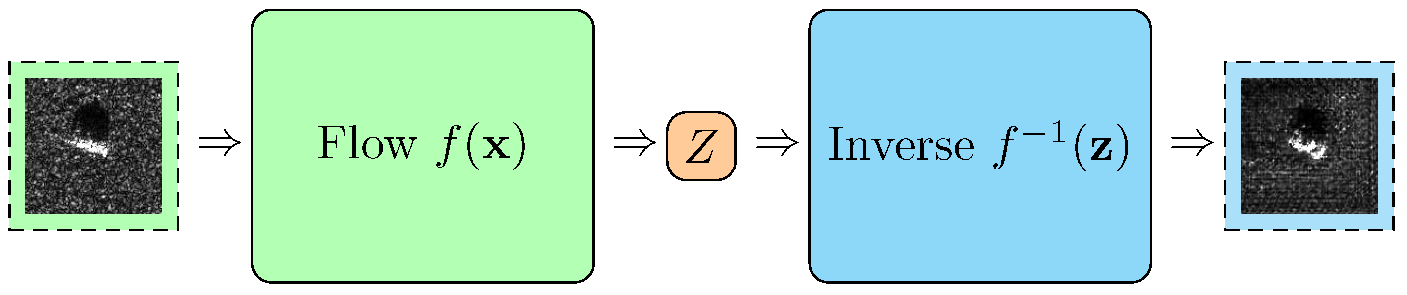
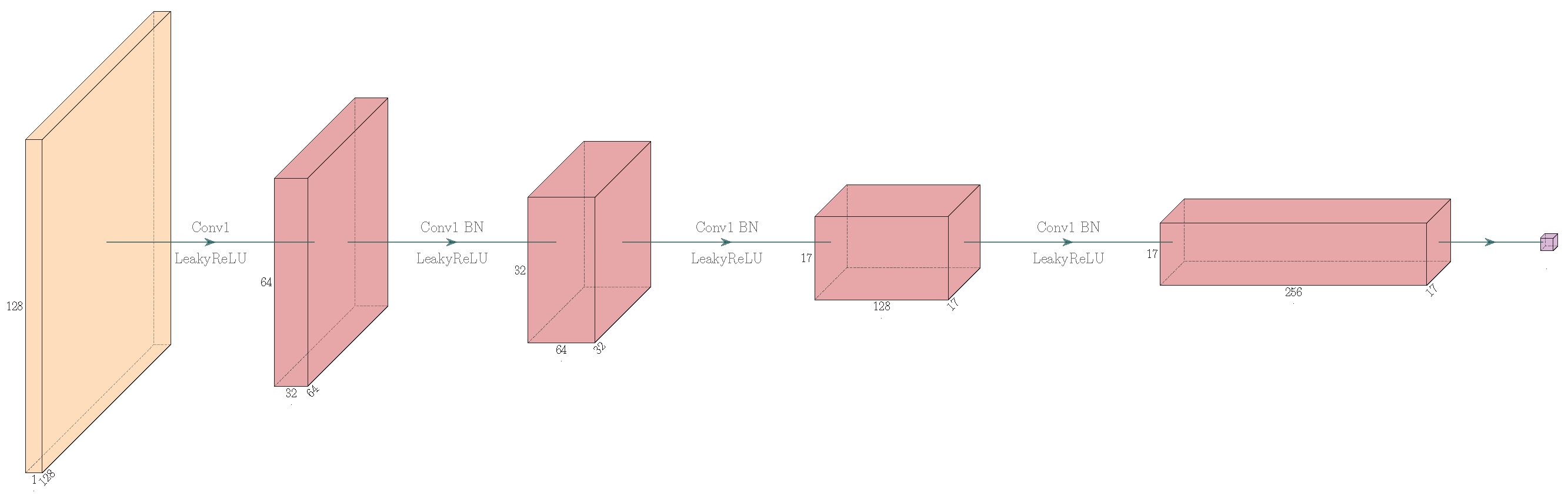
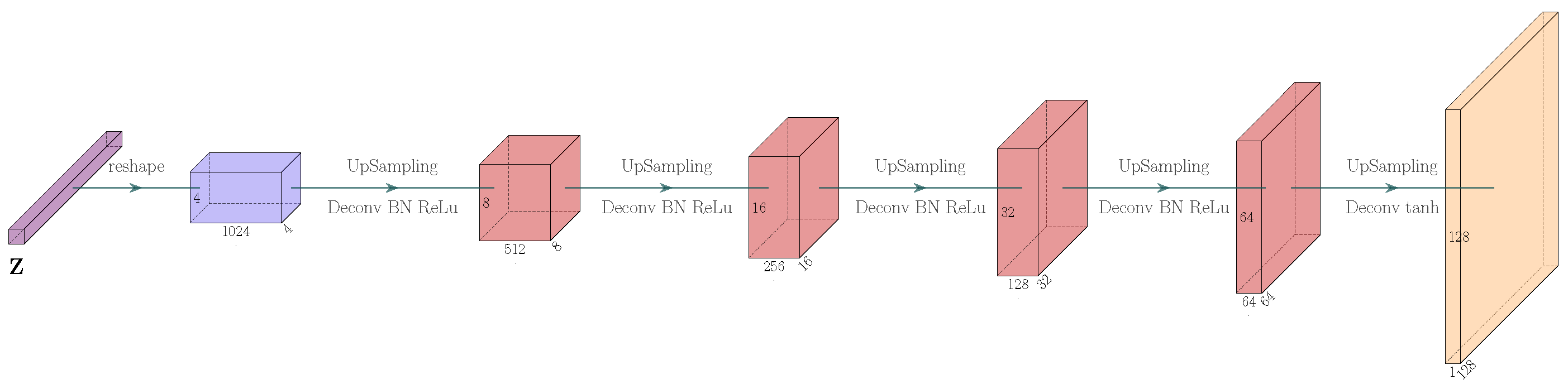
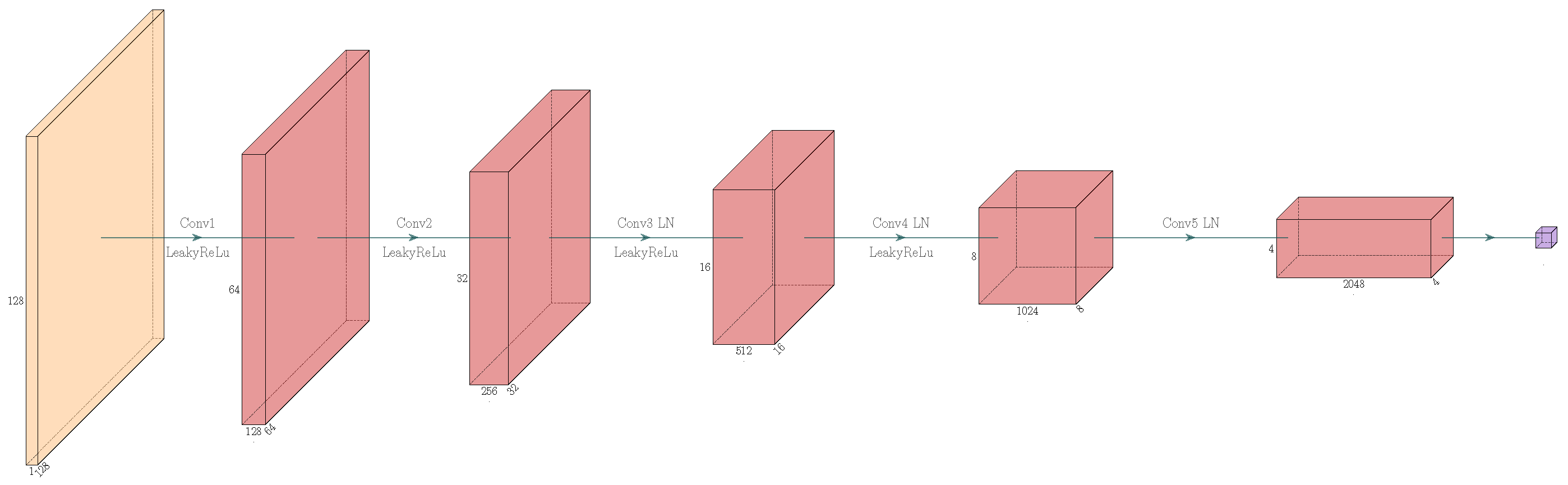
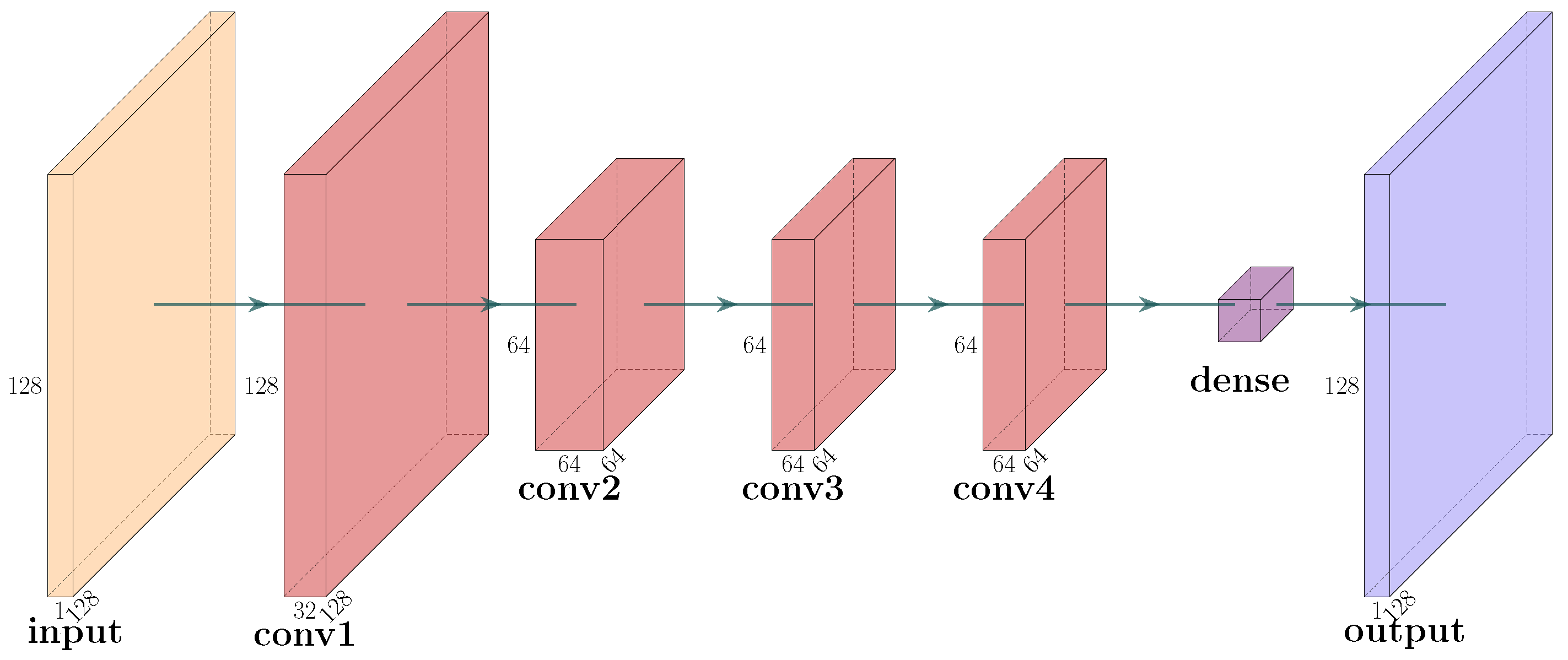
2.2. Simulation via Deep Generative Models
2.2.1. The Family of Adversarial Model
2.2.2. The Family of Variational Model
2.2.3. The Family of Flow-Based Model
3. The Proposed Strategy
3.1. Sample-Wise Assessment
- The feature extraction of simulated and real SAR images.
- Calculation of similarity and construction of fuzzy relationship matrix.
- Establishment of a FCE SAR simulated images evaluation model and obtaining evaluation result.
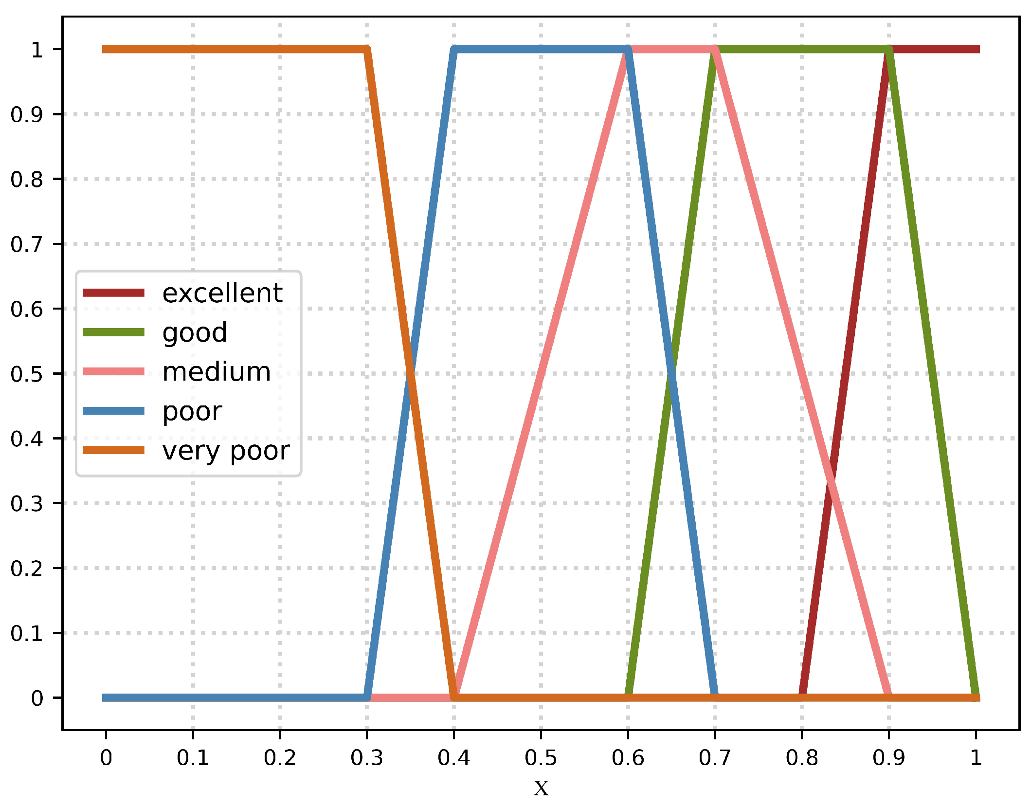
3.1.1. Construction of Evaluation Indicators
- MeanThe average pixel value of the entire image is defined as mean. Its calculation formula of a image with a size is:
- VarianceThe variance represents the unevenness of the image and reflects the fluctuation of gray value. For image of size, it can be defined as:
- Radiation resolutionRadiation resolution is a measure of image gray resolution and reflects the ability of target backscatter coefficient.The higher the radiation resolution, the higher the image quality.
- EntropyEntropy is a statistics based on information theory. For an image with a size , Its entropy is defined as:Smaller entropy means more information and better quality of the image.
3.1.2. Evaluation Model
Evaluation Set
The Weight
Fuzzy Membership Function

3.1.3. Evaluation Results
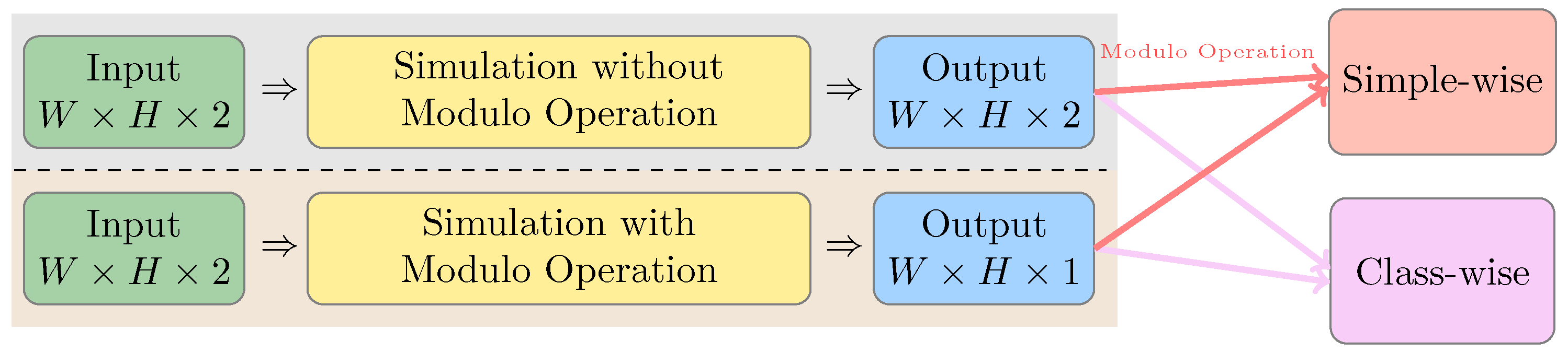
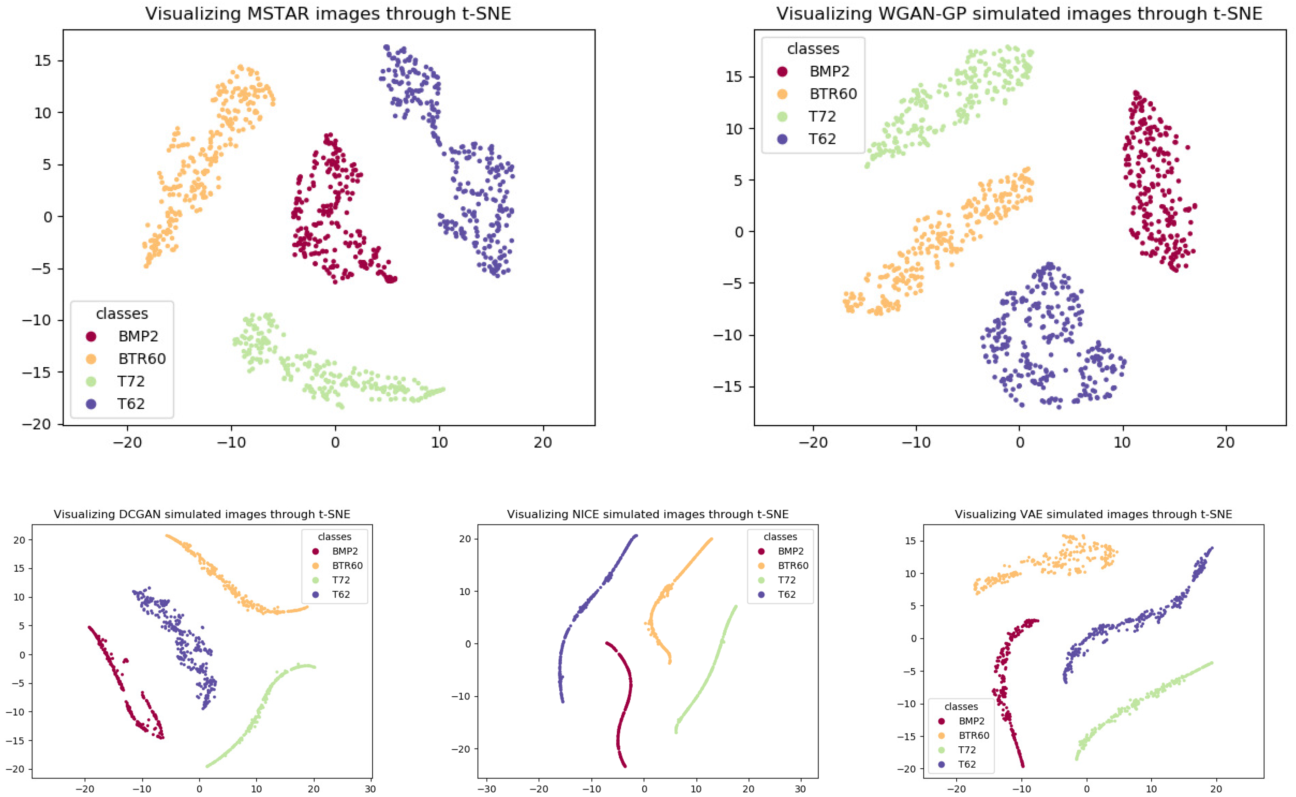
3.2. Class-Wise Assessment
3.3. Discussion
4. Experiments and Discussion
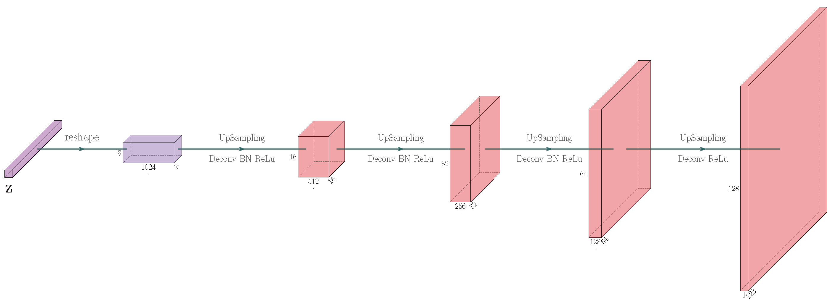
4.1. Settings and Simulation
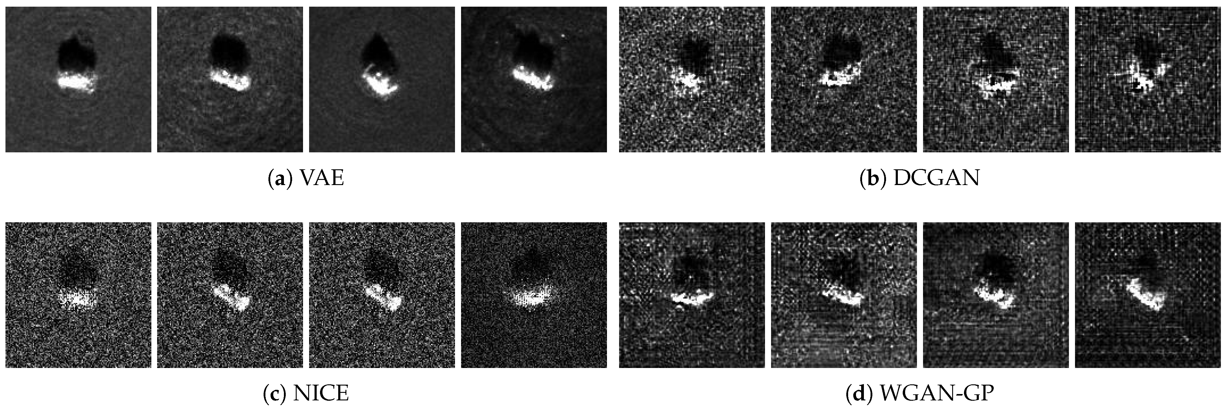
4.2. Simple-Wise
- (a)
- For each category and each model, there are no evaluations with poor and very poor, and a few medium evaluations. It shows that the effect of simulation is good.
- (b)
- NICE, WGAN-GP, and DCGAN have relatively similar results.
- (c)
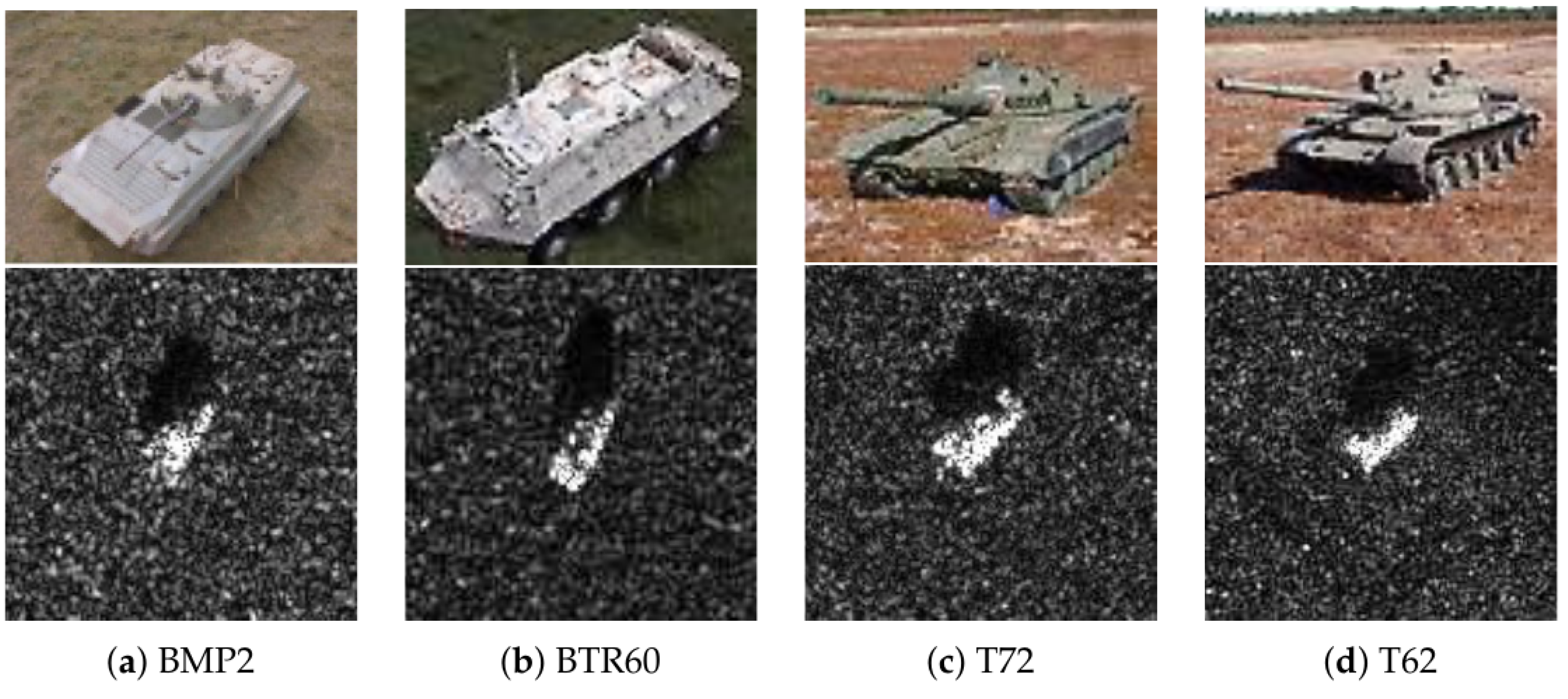
- For the four models, the evaluations of BMP2 have relatively poor results, and the evaluations of T62 are the best.
- (d)
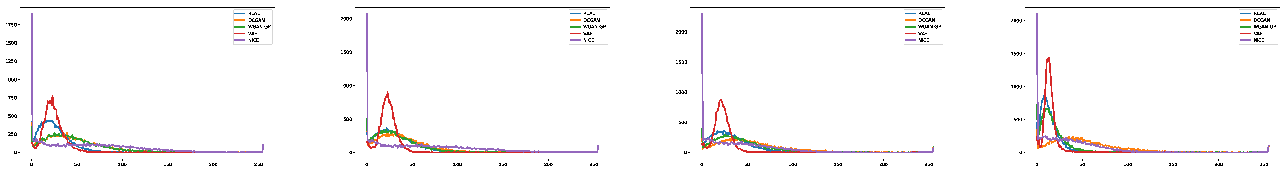
- VAE has the lowest number of excellent.This is probably because VAE does not well retain the clarity of the original images.
- (e)
- The rate of excellence in NICE is highest. This shows that the simulated images preserve the backscattering coefficient.
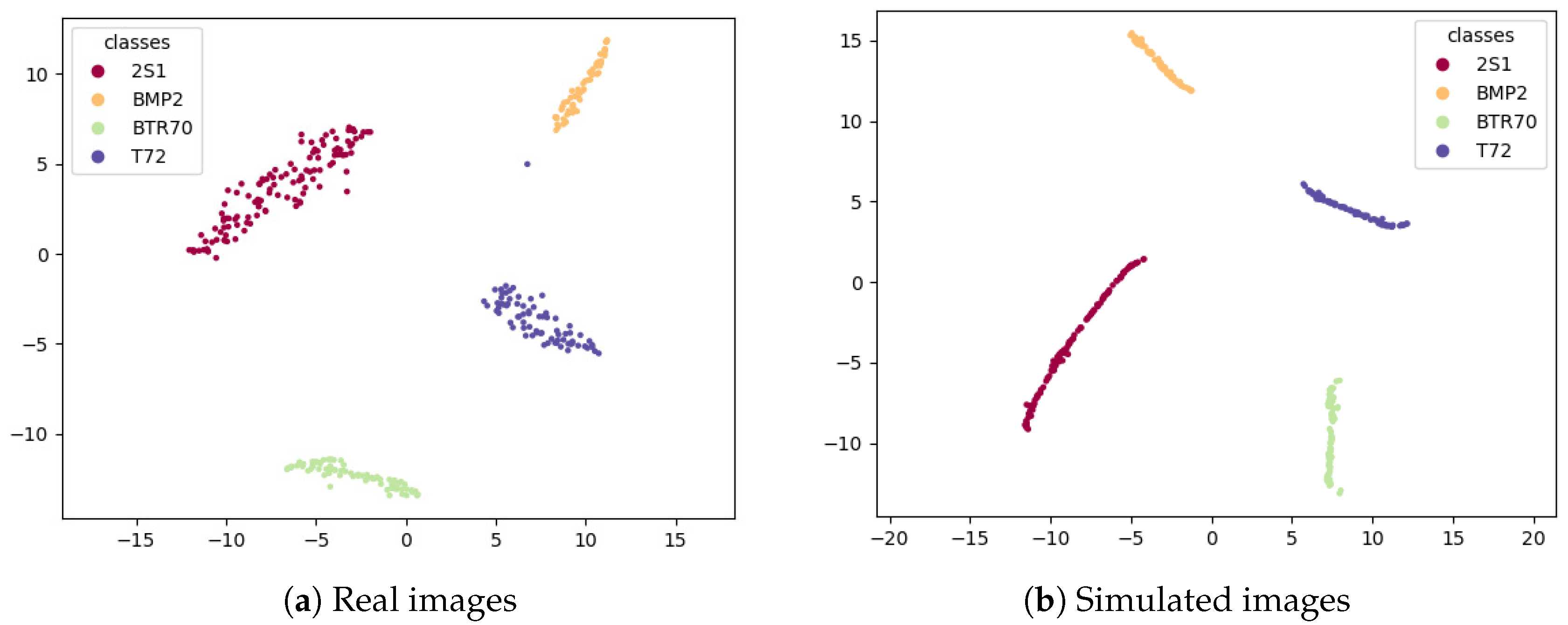
4.3. Class-Wise
4.3.1. Electromagnetic Computational Tools
4.3.2. Deep Generative Models
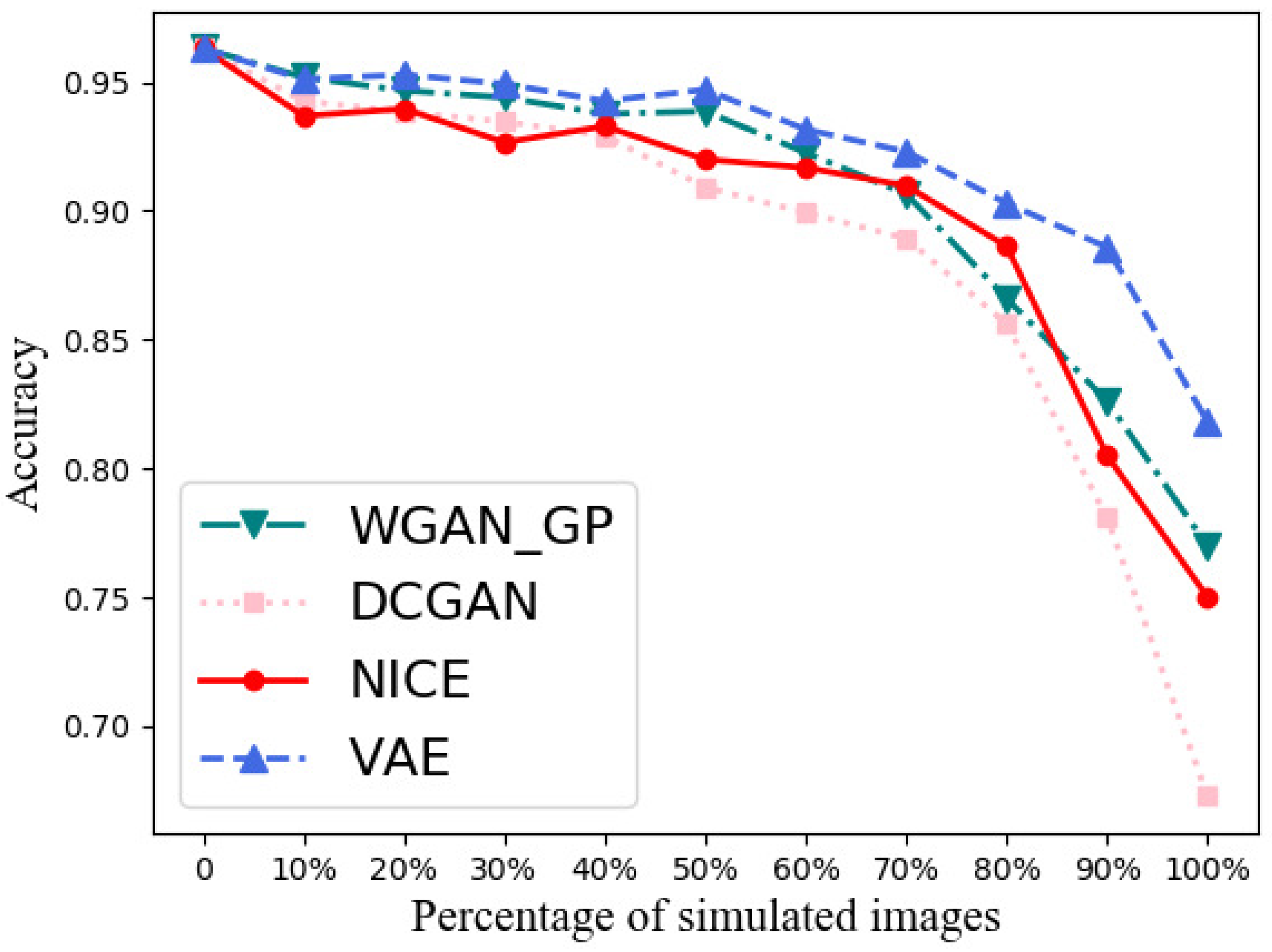
- (a)
- Without simulated images, the recognition accuracy achieves 96.30%.
- (b)
- The recognition rates of simulated datasets are 76.99%, 67.28%, 75.00%, and 81.80%.
- (c)
- The accuracy of VAE is the highest. It means that the images simulated by VAE have better application capabilities.
- (d)
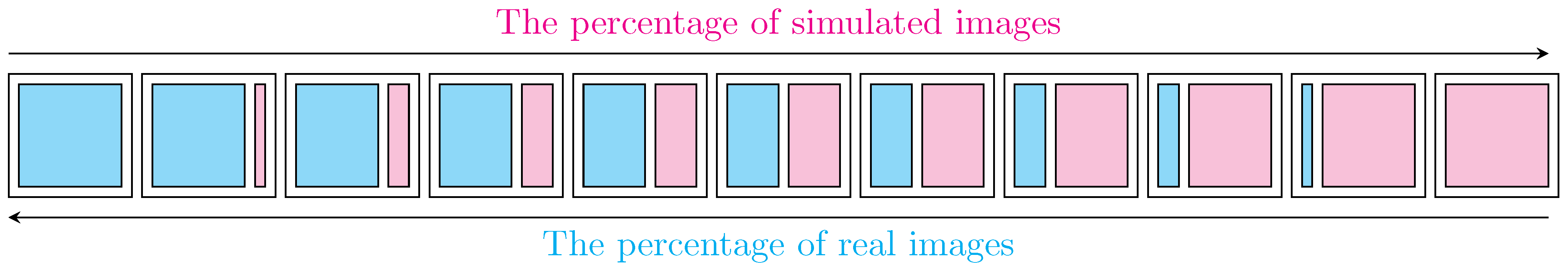
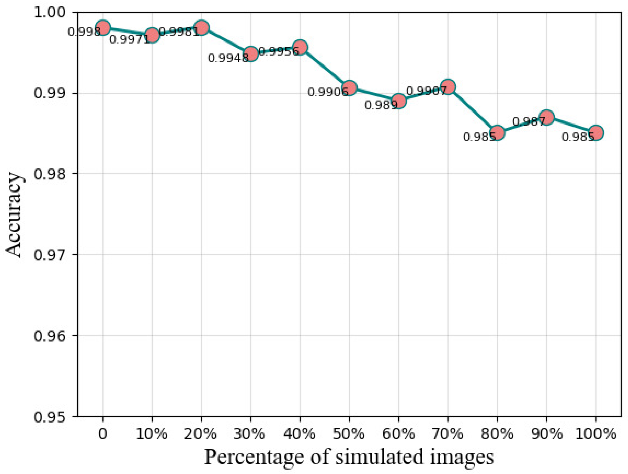
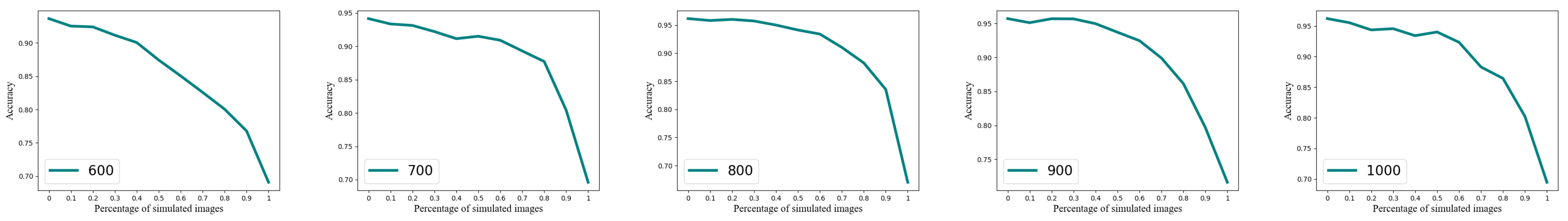
- When the percetage of simulated images is lower than 50%, the fluctuation of the accuracy is small and the values are all higher than 90%. These prove the simulated images can be used to augment the dataset in classification tasks.
4.3.3. The Effect of Dataset Size
4.4. Comparison with Other Criteria
4.5. Comprehensive Analysis
5. Conclusions
Author Contributions
Funding
Conflicts of Interest
References
- Wang, K.; Zhang, G.; Leung, H. SAR Target Recognition Based on Cross-Domain and Cross-Task Transfer Learning. IEEE Access 2019, 7, 153391–153399. [Google Scholar] [CrossRef]
- Xu, Q.; Huang, G.; Yuan, Y.; Guo, C.; Sun, Y.; Wu, F.; Weinberger, K. An empirical study on evaluation metrics of generative adversarial networks. arXiv 2018, arXiv:1806.07755. [Google Scholar]
- Heusel, M.; Ramsauer, H.; Unterthiner, T.; Nessler, B.; Hochreiter, S. Gans trained by a two time-scale update rule converge to a local nash equilibrium. Adv. Neural Inf. Process. Syst. 2017, 30, 6629–6640. [Google Scholar]
- Wang, Z.; Bovik, A.C.; Sheikh, H.R.; Simoncelli, E.P. Image quality assessment: From error visibility to structural similarity. IEEE Trans. Image Process. 2004, 13, 600–612. [Google Scholar] [CrossRef]
- Yoo, J.; Kim, J. SAR Image Generation of Ground Targets for Automatic Target Recognition Using Indirect Information. IEEE Access 2021, 9, 27003–27014. [Google Scholar] [CrossRef]
- Nie, C.; Kong, Y.; Leung, H.; Yan, S. Evaluation methods of similarity between simulated SAR images and real SAR images. In Proceedings of the 2016 CIE International Conference on Radar (RADAR), Guangzhou, China, 10–13 October 2016; pp. 1–4. [Google Scholar]
- Yu, Z.; Dong, G. A New Quantitative Evaluation Strategy for Deep Generated Sar Images. In Proceedings of the IGARSS 2022—2022 IEEE International Geoscience and Remote Sensing Symposium, Kuala Lumpur, Malaysia, 17–22 July 2022; pp. 2626–2629. [Google Scholar]
- Niu, S.; Qiu, X.; Lei, B.; Ding, C.; Fu, K. Parameter Extraction Based on Deep Neural Network for SAR Target Simulation. IEEE Trans. Geosci. Remote Sens. 2020, 58, 1–14. [Google Scholar] [CrossRef]
- Goodfellow, I.; Pouget-Abadie, J.; Mirza, M.; Xu, B.; Warde-Farley, D.; Ozair, S.; Courville, A.; Bengio, Y. Generative adversarial networks. Commun. ACM 2020, 63, 139–144. [Google Scholar] [CrossRef]
- Radford, A.; Metz, L.; Chintala, S. Unsupervised representation learning with deep convolutional generative adversarial networks. arXiv 2015, arXiv:1511.06434. [Google Scholar]
- Tolstikhin, I.; Bousquet, O.; Gelly, S.; Schoelkopf, B. Wasserstein auto-encoders. arXiv 2017, arXiv:1711.01558. [Google Scholar]
- Gulrajani, I.; Ahmed, F.; Arjovsky, M.; Dumoulin, V.; Courville, A. Improved training of wasserstein gans. arXiv 2017, arXiv:1704.00028. [Google Scholar]
- Cui, Z.; Zhang, M.; Cao, Z.; Cao, C. Image Data Augmentation for SAR Sensor via Generative Adversarial Nets. IEEE Access 2019, 7, 42255–42268. [Google Scholar] [CrossRef]
- Cao, C.; Cao, Z.; Cui, Z. LDGAN: A Synthetic Aperture Radar Image Generation Method for Automatic Target Recognition. IEEE Trans. Geosci. Remote Sens. 2020, 58, 3495–3508. [Google Scholar] [CrossRef]
- Xie, D.; Ma, J.; Li, Y.; Liu, X. Data Augmentation of Sar Sensor Image via Information Maximizing Generative Adversarial Net. In Proceedings of the 2021 IEEE 4th International Conference on Electronic Information and Communication Technology (ICEICT), Xi’an, China, 18–20 August 2021; pp. 454–458. [Google Scholar]
- Kingma, D.P.; Welling, M. Auto-encoding variational bayes. arXiv 2013, arXiv:1312.6114. [Google Scholar]
- Dinh, L.; Krueger, D.; Bengio, Y. Nice: Non-linear independent components estimation. arXiv 2014, arXiv:1410.8516. [Google Scholar]
- Dinh, L.; Sohl-Dickstein, J.; Bengio, S. Density estimation using Real NVP. arXiv 2016, arXiv:1605.08803. [Google Scholar]
- Kingma, D.P.; Dhariwal, P. Glow: Generative flow with invertible 1 × 1 convolutions. Adv. Neural Inf. Process. Syst. 2018, 31, 10215–10224. [Google Scholar]
- Yu, Z.; Dong, G. Similarity Analysis of Simulated SAR Target Images. In Proceedings of the 2022 30th European Signal Processing Conference (EU-SIPCO), Belgrade, Serbia, 29 August–2 September 2022; pp. 588–592. [Google Scholar]
- Huo, W.; Huang, Y.; Pei, J.; Liu, X.; Yang, J. Virtual SAR target image generation and similarity. In Proceedings of the 2016 IEEE International Geoscience and Remote Sensing Symposium (IGARSS), Beijing, China, 10–15 July 2016; pp. 914–917. [Google Scholar]
- Mu, H.; Zhang, Y.; Ding, C.; Jiang, Y.; Er, M.H.; Kot, A.C. DeepImaging: A Ground Moving Target Imaging Based on CNN for SAR-GMTI System. IEEE Geosci. Remote Sens. Lett. 2021, 18, 117–121. [Google Scholar] [CrossRef]
- Oveis, A.H.; Giusti, E.; Ghio, S.; Martorella, M. CNN for Radial Velocity and Range Components Estimation of Ground Moving Targets in SAR. In Proceedings of the 2021 IEEE Radar Conference (RadarConf21), Atlanta, GA, USA, 8–14 May 2021; pp. 1–6. [Google Scholar]
- Lewis, B.; Scarnati, T.; Sudkamp, E.; Nehrbass, J.; Rosencrantz, S.; Zelnio, E. A SAR dataset for a TR development: The Synthetic and Measured Paired Labeled Experiment (SAMPLE). In Algorithms for Synthetic Aperture Radar Imagery XXVI; SPIE: Bellingham, WA, USA, 2019; Volume 10987, pp. 39–54. [Google Scholar]
- Sugawara, Y.; Shiota, S.; Kiya, H. Super-Resolution Using Convolutional Neural Networks without Any Checkerboard Artifacts. In Proceedings of the 2018 25th IEEE International Conference on Image Processing (ICIP), Athens, Greece, 7–10 October 2018; pp. 66–70. [Google Scholar]
- Howard, A.G.; Zhu, M.; Chen, B.; Kalenichenko, D.; Wang, W.; Weyand, T.; Andreetto, M.; Adam, H. Mobilenets: Efficient convolutional neural networks for mobile vision applications. arXiv 2017, arXiv:1704.04861. [Google Scholar]
- Van der Maaten, L.; Hinton, G. Visualizing data using t-SNE. J. Mach. Learn. Res. 2008, 9, 2579–2605. [Google Scholar]
- Theis, L.; van den Oord, A.; Bethge, M. A note on the evaluation of generative models. arXiv 2015, arXiv:1511.01844. [Google Scholar]


| Target | Class | The Number of Samples | |
|---|---|---|---|
| Training Set (17°) | Testing Set (15°) | ||
| BMP2 | SN_9563 | 233 | — |
| SN_9566 | — | 196 | |
| SN_c21 | — | 196 | |
| BTR60 | — | 256 | 195 |
| T72 | SN_132 | 232 | — |
| SN_812 | — | 195 | |
| SN_s7 | — | 191 | |
| T62 | — | 299 | 273 |
| Total | 1020 | 1246 | |
| Class | Real | Smulated | Total |
|---|---|---|---|
| 2S1 | 177 | 177 | 354 |
| BMP2 | 108 | 108 | 216 |
| BTR70 | 96 | 96 | 192 |
| T72 | 110 | 110 | 220 |
| Total | 491 | 491 | 982 |
| A | ||||
|---|---|---|---|---|
| Model | Class | Excellent | Good | Medium | Poor | Very Poor |
|---|---|---|---|---|---|---|
| VAE | BMP2 | 25 | 74 | 1 | 0 | 0 |
| BTR60 | 21 | 78 | 1 | 0 | 0 | |
| T72 | 22 | 78 | 0 | 0 | 0 | |
| T62 | 74 | 26 | 0 | 0 | 0 | |
| NICE | BMP2 | 93 | 6 | 1 | 0 | 0 |
| BTR60 | 96 | 4 | 0 | 0 | 0 | |
| T72 | 97 | 3 | 0 | 0 | 0 | |
| T62 | 99 | 1 | 0 | 0 | 0 | |
| DCGAN | BMP2 | 71 | 20 | 9 | 0 | 0 |
| BTR60 | 87 | 7 | 6 | 0 | 0 | |
| T72 | 95 | 3 | 2 | 0 | 0 | |
| T62 | 98 | 2 | 0 | 0 | 0 | |
| WGAN-GP | BMP2 | 95 | 4 | 1 | 0 | 0 |
| BTR60 | 97 | 3 | 0 | 0 | 0 | |
| T72 | 87 | 13 | 0 | 0 | 0 | |
| T62 | 98 | 2 | 0 | 0 | 0 |
| Model | Variance |
|---|---|
| VAE | 0.001618 |
| NICE | 0.003742 |
| WGAN-GP | 0.003392 |
| DCGAN | 0.006746 |
Disclaimer/Publisher’s Note: The statements, opinions and data contained in all publications are solely those of the individual author(s) and contributor(s) and not of MDPI and/or the editor(s). MDPI and/or the editor(s) disclaim responsibility for any injury to people or property resulting from any ideas, methods, instructions or products referred to in the content. |
© 2023 by the authors. Licensee MDPI, Basel, Switzerland. This article is an open access article distributed under the terms and conditions of the Creative Commons Attribution (CC BY) license (https://creativecommons.org/licenses/by/4.0/).
Share and Cite
Yu, Z.; Dong, G.; Liu, H. SAR Image Quality Assessment: From Sample-Wise to Class-Wise. Remote Sens. 2023, 15, 2110. https://doi.org/10.3390/rs15082110
Yu Z, Dong G, Liu H. SAR Image Quality Assessment: From Sample-Wise to Class-Wise. Remote Sensing. 2023; 15(8):2110. https://doi.org/10.3390/rs15082110
Chicago/Turabian StyleYu, Ziyi, Ganggang Dong, and Hongwei Liu. 2023. "SAR Image Quality Assessment: From Sample-Wise to Class-Wise" Remote Sensing 15, no. 8: 2110. https://doi.org/10.3390/rs15082110