1. Introduction
Drought is a significant factor in minimizing the production of food worldwide. In agriculture, a lack of soil water directly causes crop water stress, which inhibits crop development and lowers production [
1,
2]. Therefore, during the first growing phases of the crop, it is crucial to precisely and promptly measure the soil water content. Research on soil moisture content estimations is becoming more and more crucial as a result of the rapid progress of remote sensing technologies [
3,
4]. Radar sensor transmits EMW to the surface of the ground and then collect data that are reflected from nearby objects [
5]. Radar waves are susceptible to the moisture level of the soil and have a significant penetration into the plant cover. Determining soil moisture contents at the field level using radar remote sensing is, therefore, extremely important [
6].
Some empirical models for retrieving soil water content are provided by examining the linear relation among ground-recorded soil water content and radar backscatter coefficient on a log scale [
7,
8]. Empirical models have been frequently employed in earlier studies because of their simplicity. The reliability of empirical studies is, however, not very high. ML techniques were developed in order to increase the precision of empirical studies for retrieving soil water content [
9,
10,
11]. ML techniques, particularly DL techniques, which offer significant prediction outputs, are required for training the networks. These approaches do not work well when taught to extract soil water content when there are just a few ground sample locations [
12,
13,
14].
Semi-empirical schemes were presented for soil moisture retrieval across vegetative regions as a middle ground between empirical and complicated techniques [
15,
16,
17]. An approximate model for the contribution of vegetation is the WCM. The model is appropriate for many types of plant layers and simplifies the intricate scattering effects among the vegetation layer and the soil layer [
18]. The WCM makes the assumption that the vegetative layer is a homogeneous medium, and it defines a parameter to characterize the properties of the vegetation layer [
19]. In previously published work, the researchers used WCM and a mix of radar and optic remote sensing data to predict soil moisture content over vegetative regions at the regional scale [
20]. In this existing research, backscatter coefficients from radar images were coupled with the soil water content to derive vegetation indices, which served as the vegetative descriptor of WCM.
The contributions are specified below:
In the initial phase, image acquisition is completed; after that, improved WCM is employed as a vegetation impact rectification scheme.
Retrieves soil moisture using DMN and Bi-GRU schemes, whose outputs are then passed on to enhance score-level fusion that offers final results.
DMN contains sufficient training data, which enables the networks to easily discriminate between different classes. While Bi-GRUs address the vanishing gradient problem are faster than other Deep learning models such as LSTM. Therefore, the combination of DMN and Bi-GRU has provided better results than other deep learning models.
The organization of this research is mentioned as follows;
Section 2 enumerates existing works on soil moisture retrieval.
Section 3 explains the phases in proposed soil moisture retrieval;
Section 4 describes the extraction of vegetation indexes. Improved WCM techniques are explained in
Section 5;
Section 6 elaborates on the concept of hybrid classifiers: DMN and BI-GRU for soil moisture retrieval. The analysis of the results and their comparisons are demonstrated in
Section 7; Lastly, the conclusion is updated in
Section 8.
2. Literature Review
2.1. Related Works
To enhance the water cloud model, Lei et al. [
21] published a novel vegetative canopy water content estimation method in 2022. Our findings demonstrated that the unique calculation method, which takes into account the canopy’s horizontal and vertical arrangement, water level, and biomass, is ideal for producing a more precise estimate of the water content of the vegetation. Additionally, the soil moisture levels of often green wood, tropical forests, diverse forest, composited shrub grasses, and grassland-enclosed regions were determined using this IWCM.
By combining the soil’s dielectric constant properties with the radar BC obtained using SA schemes of RISAT-1 data, Kishan et al. [
22] assessed SM in 2017. In order to overcome the limitations of the land surface model on the accuracy of the SM estimation, the limitations of point measurement’s spatial coverage, and the limitations of micro-wave temporal-spatial sampling, we lowered complexities through a mixture of these schemes. We looked into the effectiveness of SA in obtaining SM in which the vegetation was not extremely high.
An SM retrieval system was created in 2016 by Qingyan et al. [
23] from multi-source fused data through the stages of flowering, joinery, sowing, and heading. The association among impact factors and backscattering simulation, depending on an integration equation model, revealed that surface roughness might be less of a factor at the sowing stage by employing the CPD. The creation of a new CPD model further enhanced the Dubois model. It was very useful to estimate SM contents at the stage of jointing maize.
The flood detection capacities of various types of soil moisture data were examined by Natthachet et al. [
24] in 2021. With a forecast time, window of 8 to 32 days, a NN built from MODIS and SMOS data is employed to forecast the occurrence of flood. The most accurate forecast is for the near term (e.g., eight days), with an average recovery rate of about 60%. The results of this research point to potential use for satellite measurements of soil moisture in improving flood surveillance and detection systems.
In 2018, Anna et al. [
25] used a case study of two Swedish regions, Västra Götaland and Värml, which experienced catastrophic floods in August 2014, to integrate the temporal and spatial soil moisture parameters into the research on flood prediction systems. Data on soil moisture are obtained through remote sensing methods, with concern on the satellites that specifically measure soil moisture, ASCAT, and SMOS. Additionally, a number of PCDs are examined, and the findings indicate that generally speaking, higher drainage density and larger slopes are associated with a higher risk of floods. The findings indicate that the approach using soil moisture satellite images holds promise for enhancing the accuracy of flooding.
In 2018, Seongkyun et al. [
26] proposed a novel SVR-based downscaling technique under all sky circumstances based on microwave, optical/infrared, and geo-location data. Derived estimations of land temperatures and NDVI from MODIS land and atmospheric products were used to acquire consistent temporal-spatial input datasets to disentangle SM surveillance. This work makes the case that spatial downscaling, a remote sensing approach, has the ability to produce higher resolution SM independent of weather and without the need for additional data. It provides information for examining hydrological, climatic, and farming variables.
In 2018, Tian et al. [
27] estimated surface SM in central Tibetan Plateau, China, using a novel soil Teff method and the AMSR-E BTs. Our assessment also revealed that the novel method does not require specially suitable variables or supplemental presumptions that simplify the data necessities for regional scale appliances. This technique is utilized to calculate the historic SM for hydrologic process research over the Tibetan regions when paired with archival BT measurements.
In order to monitor droughts across India in 2022, Likithet al. [
28] investigated the possibilities of remotely sensed VOD, SIF, and SM. Utilizing time series and correlation analysis, rainfall meters such as the standardized Zscore and rainfall index were utilized to compare the Zscores of the satellite data with the Zscores of deficiency and normal rainfall events. According to the findings, SM was capable of recording drought events over all of India’s geographical areas. All three variables should be used in India’s actual drought monitoring programs since they have the potential to record drought episodes.
2.2. Review
The water cycle, ecology, and energy exchanges between the soil and the environment are all profoundly impacted by SM, an essential state variable. A variety of sectors, including meteorology, hydrology, climate, and agriculture, benefit from the use of SM data [
29,
30]. The advancement of remote sensing techniques has opened up new prospects recently in the large-scale arena. The focus of a recent study has been surfacing SM inversion using remote sensing technologies. Clouds and rain are easily blocked by distant optical sensing, which is thus easily constrained by weather and sunlight conditions. As a result, it is not possible to see the Earth under all weather conditions in the thermal and optical spectral range. Microwave remote sensing, on the other hand, is not impacted by weather or lighting condition and can detect surface SM in all seasons and at all times of the day [
31].
Additionally, because of its capacity to penetrate some types of vegetation, it has the potential to continuously monitor surface SM across a vast region. SAR was the main active electromagnetic remote sensing tool for SM monitoring throughout the last few decades. However, in places with vegetation, the signal also experiences weakened backscatter from the ground as well as direct scattering from vegetative cover. As a result, it is very challenging to extract SM when there is a plant cover since the detected backscattering signal simultaneously contains the vegetation, the surface, and the interactions among the vegetation and the surface.
The influence of surface roughness and vegetative cover must thus be eliminated in order to accurately estimate SM vegetation coverage. Different answers to the problem of how vegetation affects radar backscattering in vegetative regions have been put forth by numerous academics. The WCM is frequently used in studies as an inversion scheme to calculate SM in greenery regions. However, the accuracy of the inversion will be impacted by the absence of soil smoothness and other pertinent information owing to the terrain, real measures (SM, soil smoothness, etc.), and other variables.
3. Phases in Proposed Soil Moisture Retrieval
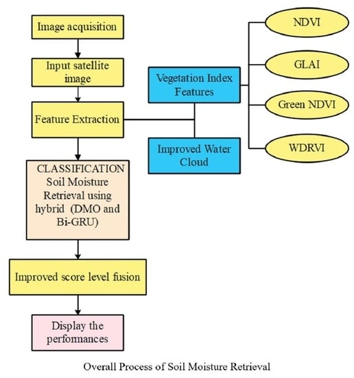
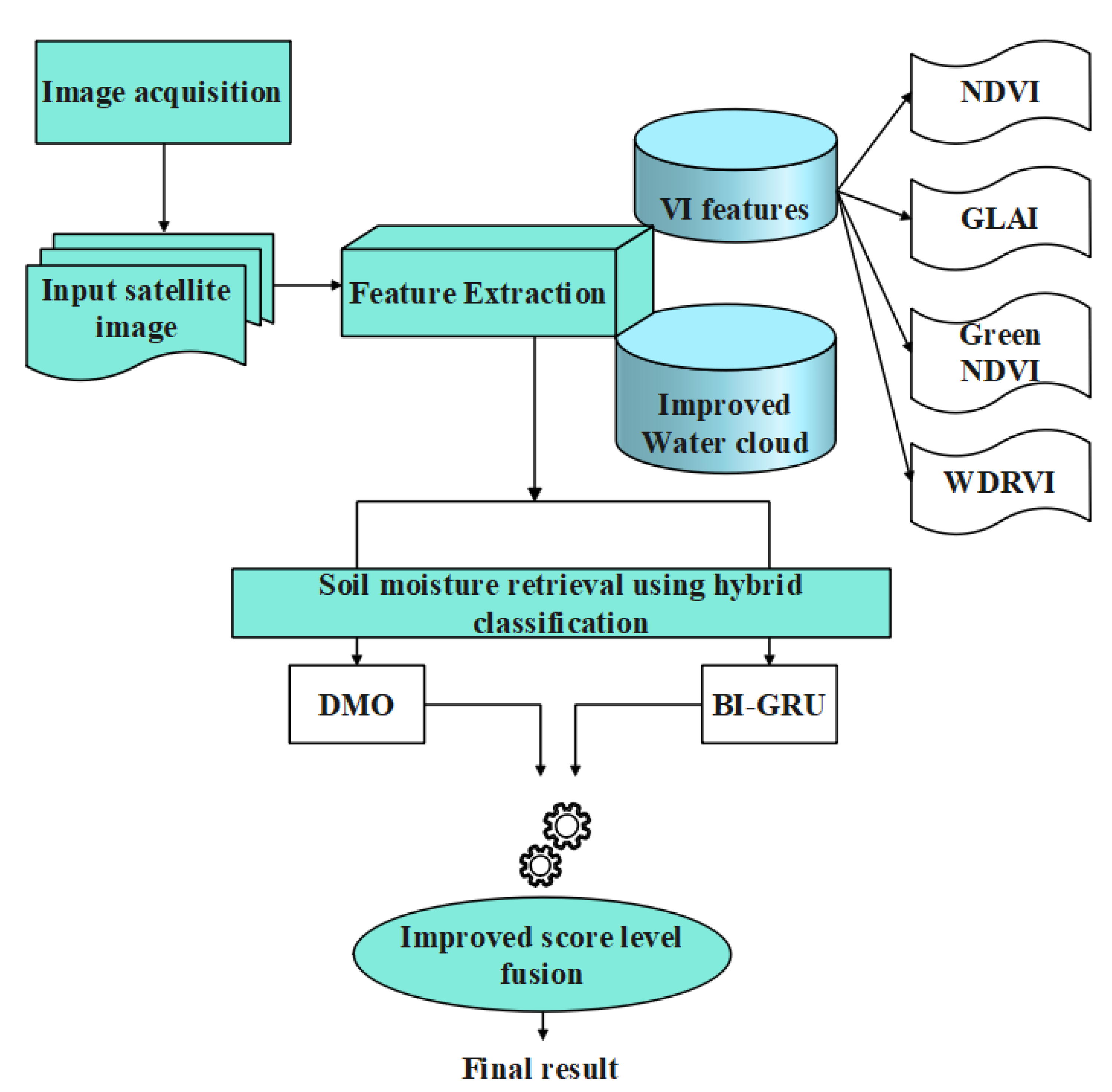
Image acquisition is carried out in the initial stage. Following that, the VI indexes (NDVI, GLAI, Green NDVI (GNDVI), and WDRVI features) are determined. Additionally, an improved Water Cloud Model (WCM) is implemented as a plan to correct the effect of vegetation. Finally, a hybrid model combining Deep Max Out Network (DMN) and Bidirectional Gated Recurrent Unit (Bi-GRU) schemes determines soil moisture retrieval. The outputs of this model are then passed on to enhanced score-level fusion, which provides the findings.
Implementing the WCM has the benefit of allowing complicated scattering characteristics in a vegetated region to be expressed with straightforward vegetation descriptors. The ideal collection of vegetation descriptors, although it has not been widely accepted or understood. In this paper, the original and improved expressions of WCM are evaluated, and the optimal vegetation descriptors are presented by examining the relationship between WCM vegetation parameters and the backscattering model predictions.
After this process, soil moisture retrieval is determined by the hybrid model combining DMN and Bi-GRU schemes. DMN contains sufficient training data, which enables the networks to easily discriminate between different classes. While Bi-GRUs address the vanishing gradient problem are faster than other Deep learning models such as LSTM. Therefore, the combination of DMN and Bi-GRU has provided better results than other deep learning models.
The steps in the adopted Soil Moisture Retrieval scheme are as follows:
In the initial phase, image acquisition is made.
Then, VI indexes (NDVI, GLAI, Green NDVI, and WDRVI features) are derived.
Further, improved WCM is deployed as a vegetation impact rectification scheme.
Finally, soil moisture is retrieved using DMN and Bi-GRU schemes, whose outputs are then passed on to enhanced score level fusion that offers final results.
The depiction of the new Soil Moisture Retrieval model is shown in
Figure 1.
Image Acquisition
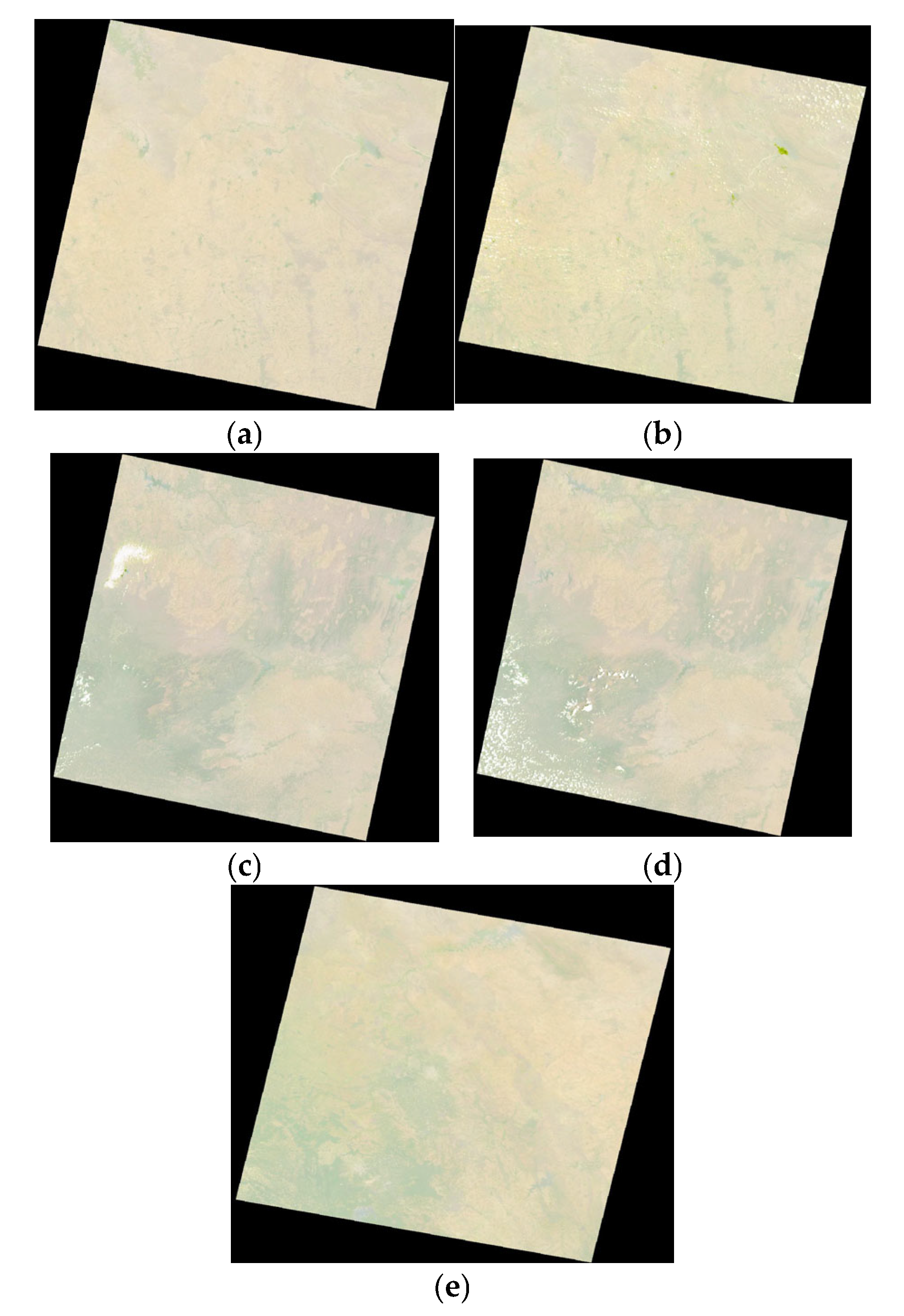
The image for analysis was collected from [
32] Sentinel-1 Data on 15 July 2017 from the city of Mumbai, India. Sentinel-1 offers high and medium-resolution land, sea ice, and coastal observations with dual and single polarization, fast revisiting cycles, and high interfering capabilities for worldwide high-resolution surveillance. Sentinel-1 has all-weather imaging abilities. Additionally, it offers technical assistance for long-term soil moisture management within the same region. From the Input image
, VI indexes, namely, NDVI, GLAI, Green NDVI, and WDRVI, are derived as the features, which are explained in the subsequent section.
4. Extraction of Vegetation Indexes
Vegetation Index values were independently calculated using ascending and descending modes on SAR data time series. One index value is calculated for each group of four consecutive SAR images for every acquisition mode. The noise in vegetation index computation was expected to be reduced by using four SAR dates to calculate one mean value. By using those mean values, NDVI and other features are calculated.
4.1. NDVI Features
NDVI features are particularly helpful for tracking vegetation from continental to global scales, because it accounts for shifting lighting circumstances, surface slope, and viewing angle. NDVI features are selected because it is an important index in agricultural organizations and academic research and evaluates vegetation health, predicts agricultural output, and maps desertification. From
, the volume and strength of vegetation on the earth’s surface are measured by the NDVI, and NDVI spatial composite pictures are created to more clearly discern between the green vegetation and barren soils. The NDVI Sensors have spectral ranges of 650 nm ± 5 nm with 65 full-width half-maximum (Red) and 810 nm ± 5 nm with 65 full-width half-maximum (NIR). The visible red band and the near-infrared band are used in NDVI [
33]. These values range between −1.0 to 1.0, with negative values denoting clouds and water and +ve values around 0 denoting bare soil. High +ve values of NDVI range from sparsely vegetated (0.1–0.5) to denser green vegetations (0.6 and greater than that). It is assessed using Equation (1). Equation (1)
and
points out the near IR portion of the EMS and the red area of EMS.
The result of an NDVI calculation for a given pixel is always a number between minus one (−1) and plus one (+1); however, the absence of green leaves yields a value that is very near to zero. A value of zero denotes the absence of vegetation, while a value near +1 (0.8–0.9) denotes the greatest potential density of green leaves. In NDVI, researchers need to examine the different colors (wavelengths) of visible and near-infrared sunlight reflected by the plants in order to calculate the density of green on a plot of land. The spectrum of sunlight is made up of many distinct wavelengths, as seen through a prism. When sunlight hits an object, some of this spectrum’s wavelengths are absorbed while others are reflected. Chlorophyll, a pigment found in plant foliage, effectively absorbs visible light (between 0.4 and 0.7 ) for photosynthesis. On the other hand, the cell structure of the leaves significantly reflects near-infrared light (between 0.7 and 1.1 ). These light wavelengths are each influenced to varying degrees by the number of leaves.
4.2. GLAI Features
GLAI features help to understand the density of green coverage in comparison with ground data. Moreover, it supports the level of photosynthesis activity of a plant and the evaporation of water from leaves. The interception of radiation and precipitation, energy conversion, and water balance are all essential factors that GLAI measures. In the end, it is an accurate measure of plant development. The GLAI [
34] defines the one-sided greenish portion of leaves for every unit lateral ground surface area as a measure of green leaf area. In order to increase grain output and adapt a genotype to a certain habitat and climatic condition, its oscillations all through the crop cycle are regarded as a critical characteristic. Furthermore, knowing the dynamics of GLAI is crucial to comprehending how crops work. Important features for breeders include the rates of leaf area development and senescence, the time of the lowest and highest GLAI, and the associated magnitude. Numerous strategies, including in-situ methodologies, remote sensing techniques, and crop models, were created to calculate GLAI [
33] as in Equation (2), where
is the soil reflectance,
is the radiance,
is the leaf angle distribution,
are canopy leaf optical properties.
The dynamics of GLAI are of prime importance to understanding the functioning of crops. Breeders should pay close attention to traits such as the leaf area’s growth and senescence rates, the timing of the minimum and maximum GLAI, and the related magnitude. In order to quantify canopy reflectance, which is susceptible to changes in the GLAI, remote sensing techniques use multispectral or hyperspectral sensors. The GLAI has been statistically related to the reflectance measured in multiple bands, which is typically combined in vegetation indices using empirical techniques. The effectiveness of this method depends on the chosen vegetation indices’ sensitivity to the GLAI as well as on confounding variables such as leaf orientation, lighting conditions, and soil properties.
4.3. Green NDVI Features
Here, these Green NVDI features are chosen because they can be used in crops with dense canopies or in more advanced stages of development. At the same time, NDVI is useful for estimating crop vigor in the early phases only.
It is related to NDVI [
35] except that it analyzes the greenish spectrum in the region of 0.54 to 0.57 microns rather than the red spectrum. As per multi-spectral data that lacks an intense red channel, this is a measure of the photosynthesis rate of the natural vegetation, and it is most frequently used to determine the moisture levels and nitrogen sources in plant leaves. It is more responsive to chlorophyll content than the NDVI index. It is utilized to evaluate old and depressed vegetation. It follows the model in Equation (3).
4.4. WDRVI Features
The WDRVI features are selected for a thorough characterization of crop physiological and phenological characteristics by increasing the dynamic range while using the same bands as the NDVI.
NDVI and WDRVI both measure near IR and red-light levels, but WDRVI is at least three times more precise because it can detect minute variations in plant canopy in moderate to high plant density, which is crucial for mature crops and crops with thick canopies [
36].
The WDRVI, termed as allows for a more thorough evaluation of crop physiologic and morphological properties by raising the dynamic range by employing identical bands as NDVI.
This research calculated four different NDVI, GLAI, Green NDVI, and WDRVI features. During the early stages of the senescence period, the canopy starts to lose water content while photosynthetic activity is still increasing. As a result, VOD, which measures the water content of the vegetation, starts to decline, while NDVI, which measures the photosynthetic activity of the vegetation, increases or stabilizes.
Accordingly, the derived NDVI, GLAI, Green NDVI, and WDRVI features are pointed out as ; .
5. Improved WCM Technique
Along with the
features, improved water cloud model-based features considered as
will be extracted. In general, the roughness, soil wetness, salt content, and vegetation all have an impact on the backscattering coefficient measured from the top of soil salinity covered in vegetation. Therefore, the plant influence needs to be eliminated in order to correctly extract the soil surface’s properties of radar backscattering. The sparse vegetation covering area is greater than the farming area in the real scenario of the radar area’s surface coverage. The vegetation impact correction model was thus chosen to be the semi-empirical WCM [
37]. The vegetative layers are homogenous and comparable in shape and size. Thus, according to two hypotheses in the water-cloud model, several scattering among plants and the surface of Earth is ignored. Equations (4)–(6) represent the WCM, respectively.
Equations (3)–(5)
refer to BC of vegetative radar layer,
refers to vegetative radar BC of the soil,
refers to 2-way vegetative radar BC at surfaces oil following attenuation,
refers to double layer attenuation feature of radar band piercing the vegetative layer,
refers to the mean water level of every vegetation in the pixels, and
as well as
refers to improvement values of vegetative moisture level constraints of diverse basic surfaces. Conventionally, the experimental constraints of all vegetation formulations were elected, such as
A = 0.0009 and
B = 0.032 [
38]. Based on an improved WCM model,
and
is evaluated using a sine map-based chaotic function.
The impact of vegetation on radar BC is exposed in Equation (7).
Conventionally, Equation (8) represents the BC of the soil subsequent to the removal of the vegetative effect.
Based upon the improved WCM model, the BC of the soil subsequent to the removal of vegetative effect is modeled based on weight
as shown in Equation (9). Here,
is computed using the mean of VI, as shown in Equation (10).
Finally, the feature set are subjected to a hybrid classifier with DMN and Bi-GRU for soil moisture retrieval.
6. Hybrid Classifiers: DMN and Bi-GRU for Soil Moisture Retrieval
As specified before, the proposed hybrid model combines the models such as DMN and Bi-GRU, where the final outcome is determined by the improved score level fusion.
6.1. DMN
The input to the DMN is
. DMN is a type of NN is DMN [
39] which finds usage in a number of applications. Each neuron contains
candidate parts that make up a NN. For neuron activation, a max value extensible
component is planned to be used. Mark
hidden layer’s
node and each of its parts as
. Equations (11) and (12) illustrate their interrelationship.
is modeled as in Equation (12).
Here, points out layer vector
refers to bias vector of layer.
and points out max-out activation vector and weight of layer.
6.2. Bi-GRU
Meanwhile,
is subjected as the input to Bi-GRU. It [
40] is a particular RNN type that helps in managing data from subsequent and earlier time steps in order to provide projected outputs depending on the present state. Equations (13)–(16) show the sigmoid function, hidden, and input vectors as
,
and
in that sequence, thus revealing the BI-GRU calculation. The reset data are denoted by
, the terms
points out weight,
points out time interval, and
points out cell condition at the preceding time stamp.
The Bi-GRU and DMN outputs and are passed to improved score-level fusion to obtain a final result.
6.3. Improved Score Level Fusion
The Bi-GRU and DMN outputs
and
are passed to improved score level fusion to obtain the final result, which is formulated as shown in Equation (17).
Equation (18)
and
refers to scores obtained from Bi-GRU and DMN. Here,
and
refers to weights that are computed using EER as shown in Equation (17). Overall, lowering the ERR value will increase the accuracy of the system. Finally,
determines the retrieval results, which are obtained using Equation (18),
7. Results and Discussion
7.1. Simulation Procedure
The deployed HC (Bi-GRU and DMN) for soil moisture retrieval was made in MATLAB. From [
32], the dataset was gathered. The evaluation was performed over Long Short-Term Memory (LSTM), Support Vector Machine (SVM), Convolutional Neural Network (CNN), Recurrent Neural Network (RNN), Naive Bayes (NB), Improved Water Cloud Model (IWCM) [
21], Solar-Induced chlorophyll Fluorescence and Vegetation Optical Depth (SIF-VOD) [
28], Basin-Scale Flood Monitoring System BSFMS [
24], AIEM model [
37] and Dubois model [
41] for diverse measures. The samples of certain collected satellite images are represented in
Figure 2.
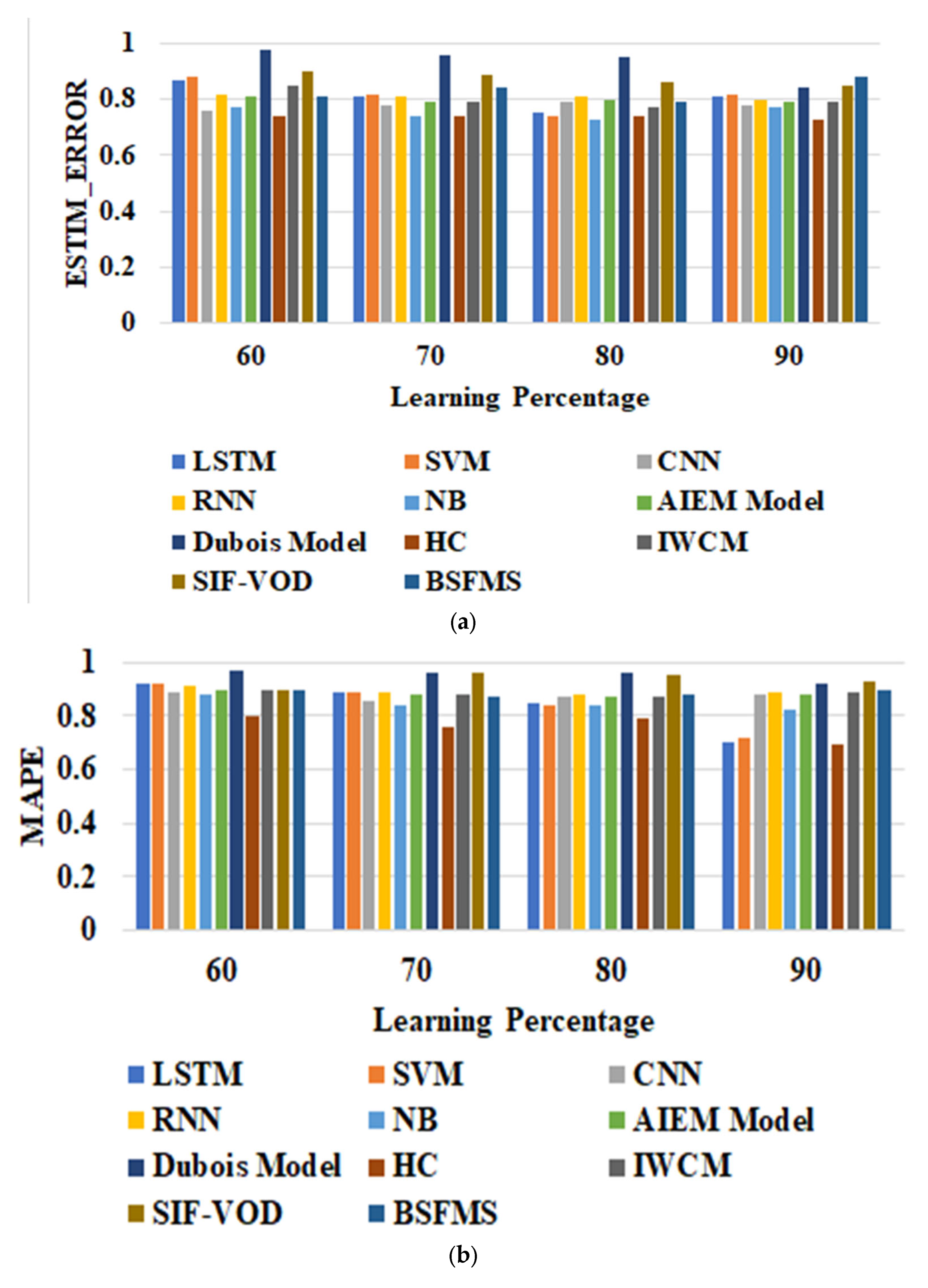
7.2. Performance Analysis
The performance of the HC (Bi-GRU and DMN) scheme for soil moisture retrieval is evaluated over LSTM, SVM, CNN, RNN, NB, AIEM model [
37], IWCM [
21], SIF-VOD [
28], BSFMS [
24] and Dubois model [
41] for error metrics in
Figure 3 and
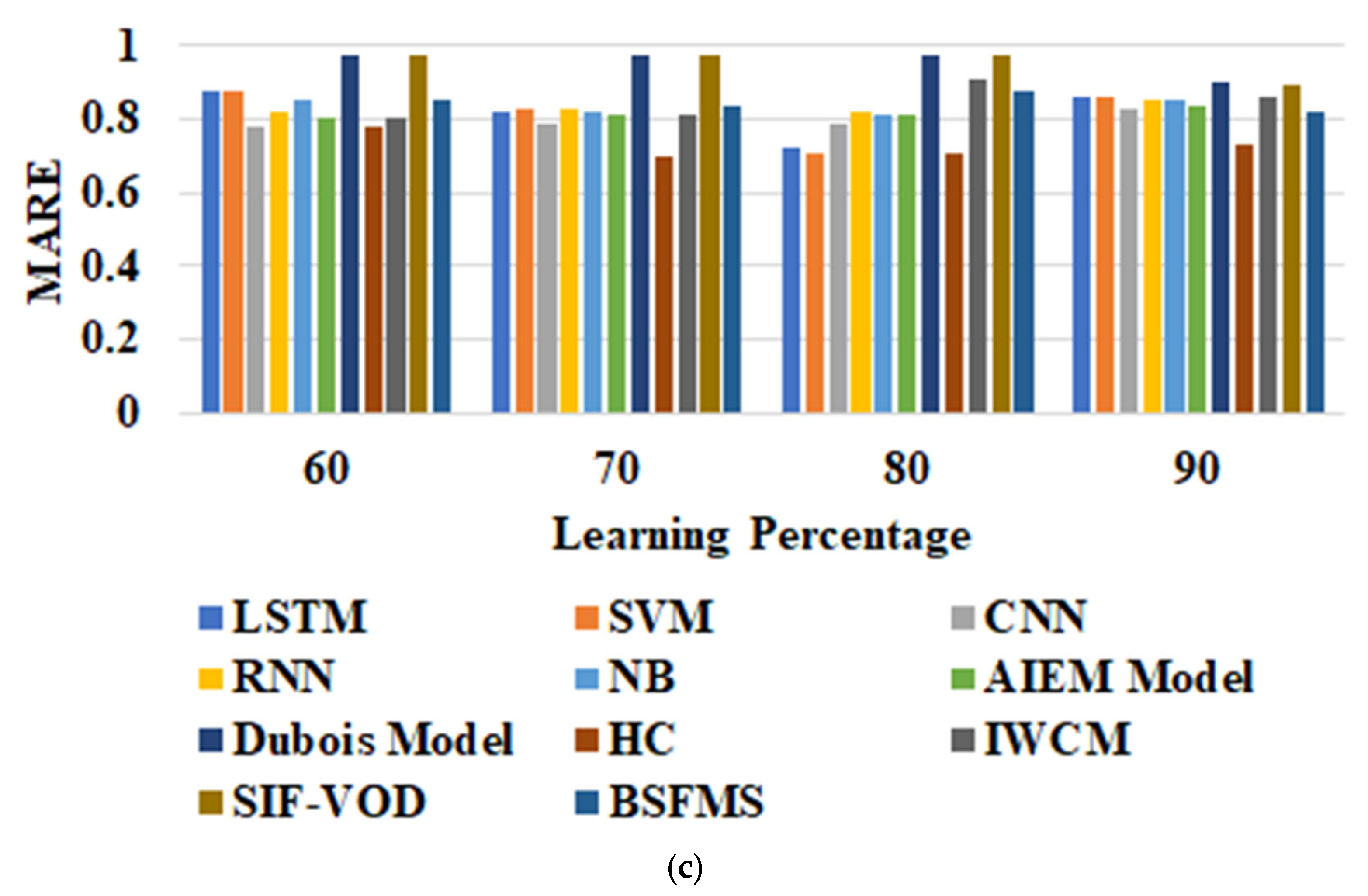
Figure 4. The analysis of HC (Bi-GRU and DMN) over conventional methods for estimated error, MAPE, and MARE is shown in
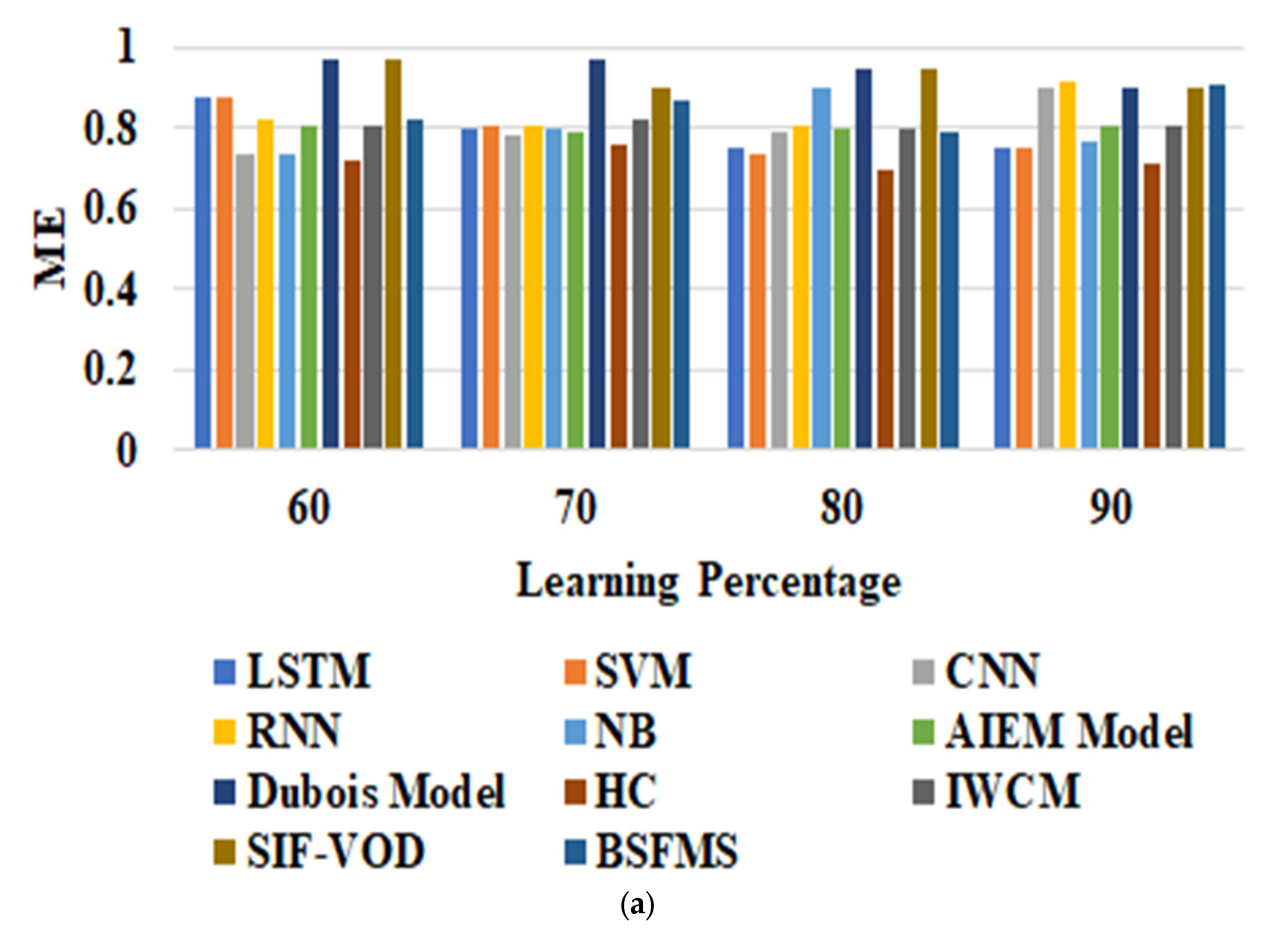
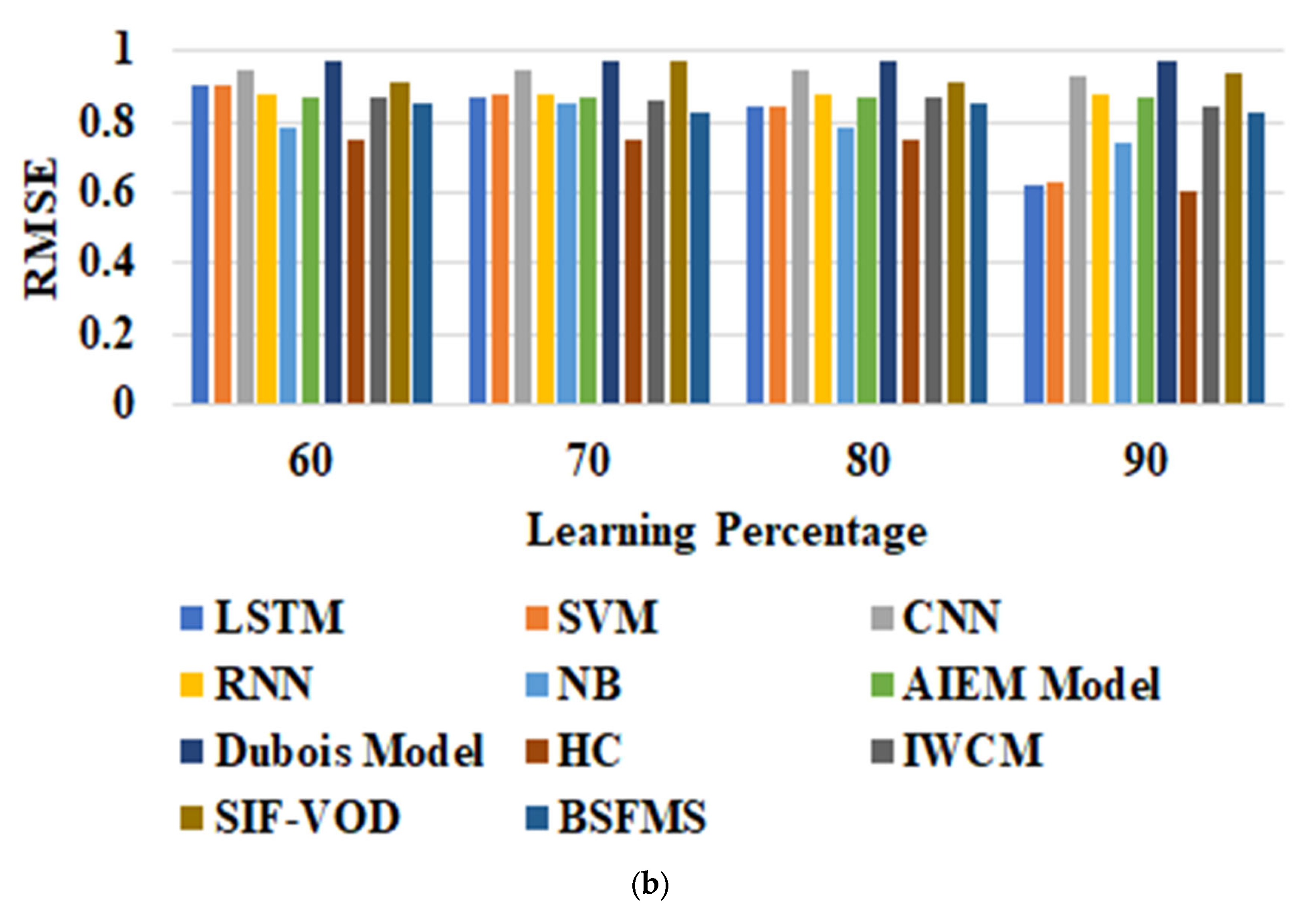
Figure 3. The analysis of HC (Bi-GRU and DMN) over conventional methods for estimated error, ME, and RMSE is shown in
Figure 4. “The mean absolute percentage error (MAPE), also known as mean absolute percentage deviation (MAPD), is a measure of prediction accuracy of a forecasting method in statistics. The relative error is a measure of the uncertainty of measurement compared to the size of the measurement. The mean error is an informal term that usually refers to the average of all the errors in a set. An error in this context is an uncertainty in a measurement or the difference between the measured value and the true/correct value. The RMSE is a frequently used measure of the differences between values (sample or population values) predicted by a model, or an estimator and the values observed. The RMSD represented the square root of the second sample moment of the differences between predicted values and observed values or the quadratic mean of these differences”.
The estimated error of the adopted HC (Bi-GRU and DMN) approach is lesser than LSTM, SVM, CNN, RNN, NB, AIEM model [
37], IWCM [
21], SIF-VOD [
28], BSFMS [
24] and Dubois model [
41] for all LPs. On the other hand, the estimated error is higher for the Dubois model [
41] for all LPs. The MAPE of HC (Bi-GRU and DMN) model 90th LP is less than the MAPE values attained at 60th, 80th, and 70th LPs. Conversely, the MAPE error is higher for the Dubois model [
41] for all LPs. Next to the 90th LP, the MAPE using HC (Bi-GRU and DMN) scheme is less at the 70th LP, while MAPE using LSTM, SVM, CNN, RNN, NB, AIEM model [
37], IWCM [
21], SIF-VOD [
28], BSFMS [
24] and Dubois model [
41] is higher for all LPs. The MARE is much negligible when using HC (Bi-GRU and DMN) scheme at the 80th LP, while the MARE is high at the 60th and 90th LPs. On the other hand, the MARE is higher than the Dubois model [
41] for all LPs. The ME using HC (Bi-GRU and DMN) scheme is much negligible at 80th LP. Next to the 80th LP, the ME is low at the 60th LP. Here, high ME is attained during the 70th LP. The RMSE at 90th LP using HC (Bi-GRU and DMN) scheme has gained a lower value of 0.65. The worst RMSE value is observed at 90th LP. The RMSE using HC (Bi-GRU and DMN) scheme is less at 90th LP. The next less value of RMSE using HC (Bi-GRU and DMN) scheme is observed at 70th LP and 60th with 0.72. The attainment of these outcomes is mainly because of HC and improved score level fusion with improved WCM.
7.3. Statistical Analysis
Table 1 shows the statistical analysis of the employed HC (Bi-GRU and DMN) model over LSTM, SVM, CNN, RNN, NB, AIEM model [
37], IWCM [
21], SIF-VOD [
28], BSFMS [
24] and Dubois model [
41]. From
Table 1, the employed HC (Bi-GRU and DMN) system established fewer error outcomes when distinguished over LSTM, SVM, CNN, RNN, NB, AIEM model [
37], IWCM [
1], SIF-VOD [
28], BSFMS [
4] and Dubois model [
41] schemes for every case. Mainly, the adopted HC (Bi-GRU and DMN) method offered lesser errors than LSTM, SVM, CNN, RNN, NB, and AIEM models [
37] and the Dubois model [
41]. This reveals that the performance of classifiers (LSTM, SVM, CNN, RNN, NB, AIEM model [
37], IWCM [
21], SIF-VOD [
28], BSFMS [
24], and Dubois model [
41]) was not better as our HC (Bi-GRU and DMN) since the compared ones pose high error values. The attainment of fewer error values is mainly because of improved WCM with HC and improved score-level fusion.
7.4. Analysis of Features
The analysis of the presented HC (Bi-GRU and DMN) system over the HC method without vegetation index, HC method without water cloud, and HC method with conventional water cloud is shown in
Table 2. In
Table 2, the estimated error of HC (Bi-GRU and DMN) is lesser than the HC method without vegetation index, HC method without water cloud, and HC method with conventional water cloud. Next to HC (Bi-GRU and DMN) scheme, the HC method without vegetation index has achieved less estimated error outcomes over the HC method without water cloud and the HC method with conventional water cloud. Moreover, the RMSE of HC (Bi-GRU and DMN) is lesser (0.956) over the HC method without vegetation index, HC method without water cloud, and HC method with conventional water cloud. Next to HC (Bi-GRU and DMN), the HC method without vegetation index has achieved fewer RMSE values than the HC method without water cloud and the HC method with conventional water cloud. Similarly, the ME values of HC (Bi-GRU and DMN) are less (0.728) over the HC method without vegetation index, HC method without water cloud, and HC method with conventional water cloud. Next to HC (Bi-GRU and DMN), the HC method without vegetation index has achieved less error of 0.821 over the HC method without water cloud and the HC method with conventional water cloud.
8. Conclusions
This paper suggested a novel technique for Soil Moisture Retrieval. In the initial phase, image acquisition was made. Then, VI indexes (NDVI, GLAI, Green NDVI, and WDRVI features) were derived. Further, improved WCM was deployed as a vegetation impact rectification scheme. At last, soil moisture was retrieved using DMN and Bi-GRU schemes, whose outputs were then passed on to enhanced score-level fusion that offered final results. From outcomes, the RMSE of HC (Bi-GRU and DMN) was lesser (0.9565) over the HC method without vegetation index, HC method without water cloud, and HC method with conventional water cloud. Next to HC (Bi-GRU and DMN), the HC method without vegetation index has achieved fewer RMSE values than the HC method without water cloud and the HC method with conventional water cloud. Similarly, the ME values of HC (Bi-GRU and DMN) were less (0.728697) over the HC method without vegetation index, HC method without water cloud, and HC method with conventional water cloud. Next to HC (Bi-GRU and DMN), the HC method without vegetation index has achieved less error of 0.8219 over the HC method without water cloud and the HC method with conventional water cloud. In the future, this research will be extended by using novel feature selection techniques to enhance overall performance.
Author Contributions
The paper investigation, resources, data curation, writing—original draft preparation, writing—review and editing, and visualization were conducted by G.S.N. and D.R.M. The paper conceptualization and software were conducted by S.S.A. and M.A. The validation and formal analysis, methodology, supervision, project administration, and funding acquisition of the version to be published were conducted by D.K.B. and J.S. All authors have read and agreed to the published version of the manuscript.
Funding
This project is funded by King Saud University, Riyadh, Saudi Arabia.
Data Availability Statement
Not applicable.
Acknowledgments
Researchers Supporting Project number (RSP2023R167), King Saud University, Riyadh, Saudi Arabia.
Conflicts of Interest
The authors declare no conflict of interest.
Nomenclature
| AIEM | Advanced Integral Equation Model |
| Bi-GRU | Bidirectional Gated Recurrent Unit |
| CNN | Convolutional Neural Network |
| DL | Deep Learning |
| HC | Hybrid Classifier |
| PCDs | Physical Catchments Descriptor |
| DMN | Deep Max Out Network |
| GNDVI | Green NDVI |
| BC | Backscattering Coefficient |
| GLAI | Green Leaf Area Index |
| EMW | ElectroMagnetic Waves |
| IWCM | Improved Water Cloud Model |
| CPD | Co-Polarized Difference |
| LSTM | Long Short Term Memory |
| IR | Infrared |
| EMS | Electro Magnetic Spectrum |
| MARE | Mean Absolute Relative Error |
| SAR | Synthetic Aperture Radar |
| LP | Learning Percentage |
| ML | Machine Learning |
| MAPE | Mean Absolute Percentage Error |
| SMOS | Soil Moisture And Ocean Salinity Mission |
| MODIS | Moderate Resolution Imaging Spectroradiometer |
| WDRVI | Wide Dynamic Range Vegetation Index |
| ME | Mean Error |
| NN | Neural Network |
| NB | Naïve Bayes |
| NDVI | Normalized Difference Vegetation Index |
| SA | Simulated Annealing |
| SM | Soil Moisture |
| EER | Equal Error Rate |
| RISAT | Radar Imaging Satellite Based on SAR Technique |
| RNN | Recurrent Neural Network |
| RMSE | Root Mean Square Error |
| SVR | Support Vector Regression |
| VOD | Vegetation Optical Depth |
| SIF | Solar-Induced Chlorophyll Fluorescence |
| Teff | Effective Temperature |
| WCM | Water Cloud Model |
| SVM | Support Vector Machine |
| VI | Vegetation Index |
References
- Rawat, K.S.; Singh, S.K. Retrieval of Surface Roughness Over Cropped Area using Modified Water Cloud Model (MWCM), Oh Model and SAR Data. J. Indian Soc. Remote Sens. 2022, 50, 735–746. [Google Scholar] [CrossRef]
- Yu, F.; Zhao, Y. A new semi-empirical model for soil moisture content retrieval by ASAR and TM data in vegetation-covered areas. Sci. China Earth Sci. 2011, 54, 1955–1964. [Google Scholar] [CrossRef]
- Srivastava, P.K.; Han, D.; Ramirez, M.R. Machine Learning Techniques for Downscaling SMOS Satellite Soil Moisture Using MODIS Land Surface Temperature for Hydrological Application. Water Resour. Manag. 2013, 27, 3127–3144. [Google Scholar] [CrossRef]
- Maduako, I.N.; Ndukwu, R.I.; Ifeanyichukwu, C. Multi-Index Soil Moisture Estimation from Satellite Earth Observations: Comparative Evaluation of the Topographic Wetness Index (TWI), the Temperature Vegetation Dryness Index (TVDI) and the Improved TVDI (iTVDI). J. Indian Soc. Remote Sens. 2017, 45, 631–642. [Google Scholar] [CrossRef]
- Jose, V.; Chandrasekar, A. Assessment of EnKF data assimilation of satellite-derived soil moisture over the Indian domain with the Noah land surface model. Theor. Appl. Clim. 2021, 146, 851–867. [Google Scholar] [CrossRef]
- Rawat, K.S.; Sehgal, V.K.; Pradhan, S. Semi-empirical model for retrieval of soil moisture using RISAT-1 C-Band SAR data over a sub-tropical semi-arid area of Rewari district, Haryana (India). J. Earth Syst. Sci. 2018, 127, 18. [Google Scholar] [CrossRef] [Green Version]
- Wang, W.; Zhang, C.; Li, F. Extracting Soil Moisture from Fengyun-3D Medium Resolution Spectral Imager-II Imagery by Using a Deep Belief Network. J. Meteorol. Res. 2020, 34, 748–759. [Google Scholar] [CrossRef]
- Muzylev, E.L.; Startseva, Z.P.; Uspensky, A.B.; Volkova, E.V. Modeling Water and Heat Balance Components for Large Agricultural Region Utilizing Information from Meteorological Satellites. Water Resour. 2018, 45, 672–684. [Google Scholar] [CrossRef]
- Peng, W.; Wang, J.; Zhang, J.; Zhang, Y. Soil moisture estimation in the transition zone from the Chengdu Plain region to the Longmen Mountains by field measurements and LANDSAT 8 OLI/TIRS-derived indices. Arab. J. Geosci. 2020, 13, 168. [Google Scholar] [CrossRef]
- Mao, K.; Zuo, Z.; Shen, X.; Xu, T.; Gao, C.; Liu, G. Retrieval of Land-surface Temperature from AMSR2 Data Using a Deep Dynamic Learning Neural Network. Chin. Geogr. Sci. 2018, 28, 1–11. [Google Scholar] [CrossRef] [Green Version]
- Liu, Q.; Du, J.; Shi, J.; Jiang, L. Analysis of spatial distribution and multi-year trend of the remotely sensed soil moisture on the Tibetan Plateau. Sci. China Earth Sci. 2013, 56, 2173–2185. [Google Scholar] [CrossRef]
- Klinke, R.; Kuechly, H.; Frick, A.; Förster, M.; Schmidt, T.; Holtgrave, A.-K.; Kleinschmit, B.; Spengler, D.; Neumann, C. Indicator-Based Soil Moisture Monitoring of Wetlands by Utilizing Sentinel and Landsat. Remote Sens. Data 2018, 86, 71–84. [Google Scholar]
- Holtgrave, A.K.; Förster, M.; Greifeneder, F.; Notarnicola, C.; Kleinschmit, B. Estimation of Soil Moisture in Vegetation-Covered Floodplains with Sentinel-1 SAR Data Using Support Vector Regression. PFG 2018, 86, 85–101. [Google Scholar] [CrossRef]
- Jin, Y. Theory and application for retrieval and fusion of spatial and temporal quantitative information from complex natural environment. Front. Earth Sci. China 2007, 1, 284–298. [Google Scholar] [CrossRef]
- Yu, F.; Li, H.; Gu, H.; Han, Y. Assimilating ASAR data for estimating soil moisture profile using an ensemble Kalman filter. Chin. Geogr. Sci. 2013, 23, 666–679. [Google Scholar] [CrossRef] [Green Version]
- Al-Bakri, J.; Suleiman, A.; Berg, A. A comparison of two models to predict soil moisture from remote sensing data of RADARSAT II. Arab. J. Geosci. 2014, 7, 4851–4860. [Google Scholar] [CrossRef]
- Zhao, S.; Wang, Q.; Li, Y.; Liu, S.; Wang, Z.; Zhu, L.; Wang, Z. An overview of satellite remote sensing technology used in China’s environmental protection. Earth Sci. Inform. 2017, 10, 137–148. [Google Scholar] [CrossRef]
- Im, J.; Park, S.; Rhee, J.; Baik, J.; Choi, M. Downscaling of AMSR-E soil moisture with MODIS products using machine learning approaches. Environ. Earth Sci. 2016, 75, 1120. [Google Scholar] [CrossRef]
- Wang, H.; Li, Z.; Zhang, W.; Ye, X.; Liu, X. A Modified Temperature-Vegetation Dryness Index (MTVDI) for Assessment of Surface Soil Moisture Based on MODIS Data. Chin. Geogr. Sci. 2022, 32, 592–605. [Google Scholar] [CrossRef]
- Li, M.; Wu, P.; Sexton, D.M.H.; Ma, Z. Potential shifts in climate zones under a future global warming scenario using soil moisture classification. Clim. Dyn. 2021, 56, 2071–2092. [Google Scholar] [CrossRef]
- Lei, J.; Yang, W.; Yang, X. Soil Moisture in a Vegetation-Covered Area Using the Improved Water Cloud Model Based on Remote Sensing. J. Indian Soc. Remote. Sens. 2022, 50, 1–11. [Google Scholar] [CrossRef]
- Kishan Singh, R.; Sehgal, V.K.; Pradhan, S.; Ray, S.S. Retrieval and validation of soil moisture from FRS-1 data set of radar imaging satellite (RISAT-1). Arab. J. Geosci. 2017, 10, 445. [Google Scholar]
- Qingyan, M.; Xie, Q.; Wang, C.; Ma, J.; Sun, Y.; Zhang, L. A fusion approach of the improved Dubois model and best canopy water retrieval models to retrieve soil moisture through all maize growth stages from Radarsat-2 and Landsat-8 data. Environ. Earth Sci. 2016, 75, 1377. [Google Scholar]
- Natthachet, T.; Forgotson, C.; Gangodagamage, C.; Forgotson, J. The analysis of using satellite soil moisture observations for flood detection, evaluating over the Thailand’s Great Flood of 2011. Nat. Hazards 2021, 108, 2879–2904. [Google Scholar]
- Anna-Klara, A.; Cavalli, M.; Hansson, K.; Koutsouris, A.J.; Crema, S.; Kalantari, Z. Soil moisture remote-sensing applications for identification of flood-prone areas along transport infrastructure. Environ. Earth Sci. 2018, 77, 533. [Google Scholar]
- Seongkyun, K.; Jeong, J.; Zohaib, M.; Choi, M. Spatial disaggregation of ASCAT soil moisture under all sky condition using support vector machine. Stoch. Environ. Res. Risk Assess. 2018, 32, 3455–3473. [Google Scholar]
- Tian, H.; Iqbal, M. Utilizing a new soil effective temperature scheme and archived satellite microwave brightness temperature data to estimate surface soil moisture in the Nagqu region, Tibetan Plateau of China. J. Arid. Land 2018, 10, 84–100. [Google Scholar] [CrossRef] [Green Version]
- Likith, M.; Harod, R.; Eswar, R. Exploring the use of satellite observations of soil moisture, solar-induced chlorophyll fluorescence and vegetation optical depth to monitor droughts across India. J. Earth Syst. Sci. 2022, 131, 94. [Google Scholar] [CrossRef]
- Ma, J.; Song, X.; Li, X.; Leng, P.; Li, S.; Zhou, F. Estimation of surface soil moisture from ASAR dual-polarized data in the middle stream of the Heihe River Basin. Wuhan Univ. J. Nat. Sci. 2013, 18, 163–170. [Google Scholar] [CrossRef]
- Yuan, S.; Wang, Y.; Quiring, S.M.; Ford, T.W.; Houston, A.L. A sensitivity study on the response of convection initiation to in situ soil moisture in the central United States. Clim. Dyn. 2020, 54, 2013–2028. [Google Scholar] [CrossRef]
- Ya, G.; Gao, M.; Wang, L.; Rozenstein, O. Soil Moisture Retrieval over a Vegetation-Covered Area Using ALOS-2 L-Band Synthetic Aperture Radar Data. Remote Sens. 2021, 13, 3894. [Google Scholar]
- Available online: https://scihub.copernicus.eu/dhus/#/home (accessed on 5 August 2022).
- Jae-Hyun, R.Y.U.; Dohyeok, O.H.; Jaeil, C.H.O. Simple method for extracting the seasonal signals of photochemical reflectance index and normalized difference vegetation index measured using a spectral reflectance sensor. J. Integr. Agric. 2021, 20, 1969–1986. [Google Scholar]
- Blancon, J.; Dutartre, D.; Tixier, M.H.; Weiss, M.; Comar, A.; Praud, S.; Baret, F. A High-Throughput Model-Assisted Method for Phenotyping Maize Green Leaf Area Index Dynamics Using Unmanned Aerial Vehicle Imagery. Front. Plant Sci. 2019, 10, 685. [Google Scholar] [CrossRef] [PubMed]
- Available online: https://www.soft.farm/en/blog/vegetation-indices-ndvi-evi-gndvi-cvi-true-color-140 (accessed on 5 August 2022).
- Available online: https://support.insights.granular.ag/hc/en-us/articles/360035214071-What-is-the-difference-between-NDVI-and-WDRVI (accessed on 5 August 2022).
- Shuai, H.; Ding, J.; Zou, J.; Liu, B.; Zhang, J.; Chen, W. Soil Moisture Retrival Based on Sentinel-1 Imagery under Sparse Vegetation Coverage. Sensors 2019, 19, 589. [Google Scholar]
- Nigara, T. Soil Salinization Monitoring Based on Synergy Monitoring Model of Remote Sensing and Electromagnetic Induction in Ugan-Kucha Delta Oasis. Ph.D. Thesis, Xinjiang University, Urumqi, China, 2014. [Google Scholar]
- Cai, M.; Shi, Y.; Liu, J. Deep maxout neural networks for speech recognition. In Proceedings of the IEEE Workshop on Automatic Speech Recognition and Understanding, Olomouc, Czech Republic, 8–12 December 2013; pp. 291–296. [Google Scholar]
- Tong, L.; Ma, H.; Lin, Q.; He, J.; Peng, L. A Novel Deep Learning Bi-GRU-I Model for Real-Time Human Activity Recognition Using Inertial Sensors. IEEE Sens. J. 2022, 22, 6164–6174. [Google Scholar] [CrossRef]
- Parida, B.R.; Pandey, A.C.; Kumar, R.; Kumar, S. Surface Soil Moisture Retrieval Using Sentinel-1 SAR Data for Crop Planning in Kosi River Basin of North Bihar. Agronomy 2022, 12, 1045. [Google Scholar] [CrossRef]
| Disclaimer/Publisher’s Note: The statements, opinions and data contained in all publications are solely those of the individual author(s) and contributor(s) and not of MDPI and/or the editor(s). MDPI and/or the editor(s) disclaim responsibility for any injury to people or property resulting from any ideas, methods, instructions or products referred to in the content. |
© 2023 by the authors. Licensee MDPI, Basel, Switzerland. This article is an open access article distributed under the terms and conditions of the Creative Commons Attribution (CC BY) license (https://creativecommons.org/licenses/by/4.0/).


 ,
, 


