1. Introduction
Surface soil moisture (SSM) is a critical land environment variable that connects agriculture, ecology, and hydrology, as well as a key parameter in hydrology, meteorology, and agricultural applications. SSM monitoring can be used to plan irrigation, monitor water quality, manage water resources, and estimate crop yield [
1,
2]. Understanding the spatial and temporal distribution and dynamic changes of SSM can help guide agricultural management.
Traditional SSM monitoring often employs the gravimetric method or the probe method. Although the precision is reasonably good and the operation is simple, it necessitates a significant amount of personnel and material resources, and is easily influenced by the surrounding environment and human variables. Furthermore, because the number of sample locations is restricted, it is hard to obtain a substantial amount of SSM information in a short period of time [
3].
Remote sensing technology offers a potent approach to detecting SSM on a broad scale and with great spatial-temporal resolution. Synthetic aperture radar (SAR) is a promising method for assessing SSM with high spatial-temporal resolution [
4,
5]. In contrast to optical remote sensing, SAR does not require sunshine, and microwave signals may penetrate the surface soil to estimate and monitor SSM in real time [
6]. SAR data demonstrate the vast potential and promising practice of mapping global SSM at medium and high spatial resolution [
7]. SAR is sensitive to the dielectric and geometric properties of the target [
8,
9]. Fung et al. [
10] built an integral equation model to estimate soil moisture. Empirical models such as the Oh model established by Oh et al. [
11] and the Dubois model established by Dubois et al. [
12] can estimate soil moisture within their effective range. Bao et al. [
13] modified the water cloud model (WCM) based on optical indicators, and introduced the vegetation index to reduce the impact of vegetation cover on SSM. Compared with empirical, semi-empirical, and theoretical models, machine learning can avoid complex physical relationships and solve nonlinear problems, and is widely used in SSM inversion. Gao et al. [
14] used Sentinel-1 and Sentinel-2 data to determine SSM using the change detection method. Guo et al. [
15] used Sentinel-1 and Sentinel-2 data to determine SSM using support vector regression (SVR) and generalized regression neural network (GRNN) methods. Datta et al. [
16] compared the applicability of different machine learning and linear regression models in SSM inversion using Sentinel-1 and Sentinel-2 data.
Because artificial neural network (ANN) has high nonlinear fitting abilities and can learn autonomously, it is increasingly being employed to solve the problem of SSM inversion. Arnicola et al. [
17] discovered that by increasing the number of input ANN characteristics, the SSM inversion accuracy may be gradually increased. Pasolli et al. [
18,
19] applied the SVR model to retrieve SSM using microwave remote sensing data. Using different input parameters can also increase the accuracy of SSM inversion. Said et al. [
20] estimated SSM using an ANN with several input parameters. Multiple regression is inferior to ANN inversion. In addition to traditional machine learning methods, many deep learning methods have also been employed in SSM monitoring in recent years. Cai et al. [
21] developed an SSM prediction model using a deep learning regression network (DNNR) with big data fitting capabilities. To obtain reliable results, the deep learning method requires a large number of training samples.
In the case of small samples, it is critical to select the suitable machine learning model and then refine the model parameters. When there are too many input factors, screening some distinctive parameters can significantly enhance the accuracy of soil moisture inversion. Lin et al. [
22] inverted the SSM of winter wheat fields using RADARSAT-2 data and polarization decomposition method to enhance the number of input factors, and used several feature selection and machine learning methods to improve the model performance and estimate SSM effectively and accurately. Zhang et al. [
23] extracted several features from passive microwave remote sensing data, optical remote sensing data, land surface model (LSM) and other auxiliary data, assessed the value of different features to SSM retrieval, and then proposed an SSM retrieval method based on random forest (RF) model.
In practical applications, most machine learning techniques require amounts of sample data to assure adequate training. When there are few training samples, the model trained with tiny samples is prone to over-fitting of small samples and under-fitting target tasks. Therefore, when the number of samples is insufficient, increasing the sample size is a crucial way to raise inversion accuracy. Based on multi-time camera-borne SAR and ground measurement data and the change detection theory, Balenzano et al. [
24] investigated the link between SSM changes and SAR signal changes of two crops in different wave bands, polarizations, and incident angles, and provided the quantitative equation that connects them, i.e., the alpha approximation method. He et al. [
25] expanded the alpha approximation approach by using a time series of L-band SAR data and simultaneous ground observations from SMAPEx-3 to retrieve SSM. Xu et al. [
26] used the alpha approximation method to augment the measured data for training the SVR model and further improved the SSM inversion accuracy. However, the input parameters and machine learning models used in these studies were specified in advance, lacking more optimizations of input parameters and inversion models to improve the SSM inversion accuracy further.
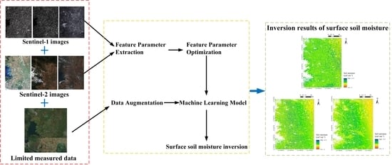
There are various constraints in SSM inversion for a small size of sample data. To improve the accuracy of SSM inversion for small samples, an SSM inversion method combining sample augmentation, feature optimization, and machine learning models was investigated in this paper. Firstly, assuming that the surface roughness and vegetation conditions remain unchanged in the short term, the field-measured SSM data were augmented by using the alpha approximation method to provide more training data for the machine learning models. Secondly, feature parameters were extracted from Sentinel-1 and Sentinel-2 remote sensing data, and optimized by using Pearson correlation analysis, RF, and principal component analysis (PCA) methods. Then, three common machine learning models suitable for small sample training, which were genetic algorithm-back propagation neural network (GA-BP), SVR, and RF, were built to retrieve SSM and evaluate the accuracy. Finally, after comparing various combinations of feature optimization methods and machine learning models, the optimal inversion model was chosen to retrieve the regional SSM of the study area.
2. Materials and Methods
2.1. Study Area and Sampling Procedures
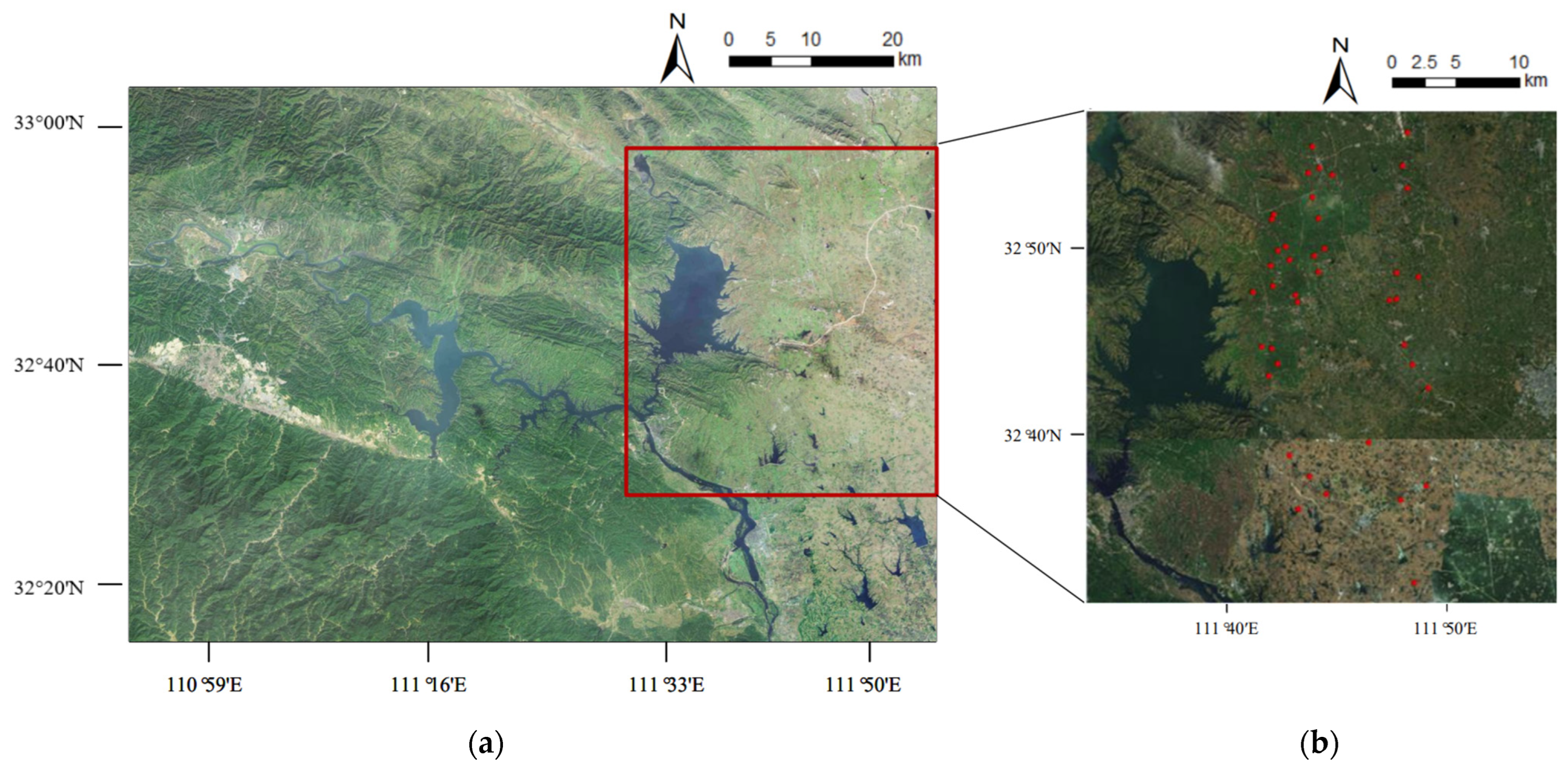
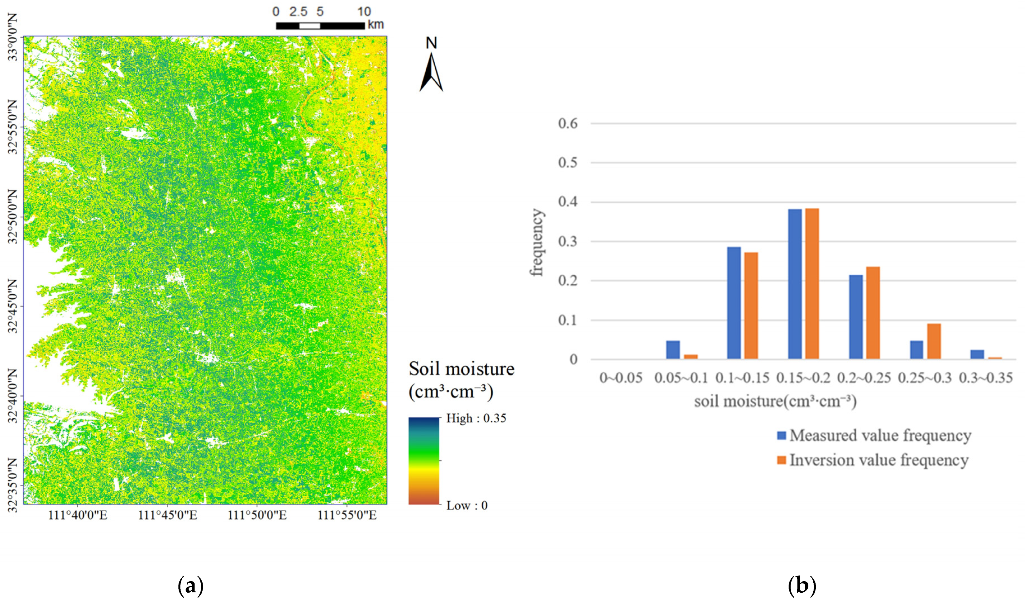
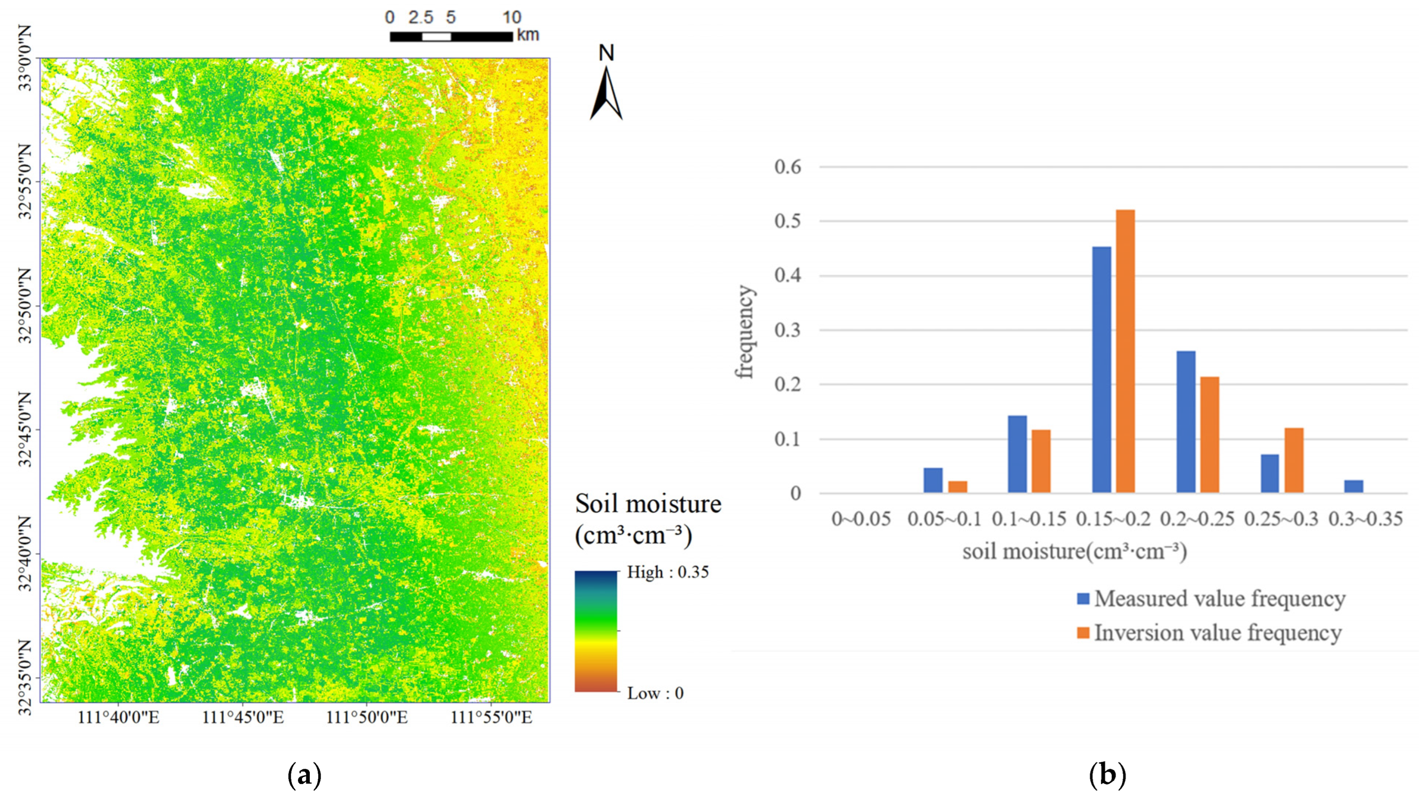
The study area was the eastern part of the Danjiangkou Ecological Service Area, which spanned Henan and Hubei provinces, China. The Danjiangkou Reservoir is the water source of the Middle Route Project of South-to-North Water Transfer. The Danjiangkou Ecological Service Area is a national first-class water source protection zone that was declared as one of China’s ecological function protection zones in 2015. Its landscape is sloping from northwest to southeast, with low mountains in the northwest, hills in the center, and hills and alluvial plains in the southeast. The soil types in the study area are mainly yellow-brown soil and brown soil [
27]. The study area has a monsoon environment ranging from the north subtropical zone to the warm temperate zone, with a mild climate, and four distinct seasons. In recent years, the annual precipitation here is about 800 mm to 1300 mm. It is a transitional zone between north and south, with a wide range of vegetation types and an abundance of plant resources. The study area is mostly made up of agricultural land, building land, and a body of water, as shown in
Figure 1.
Sentinel-1 SAR remote sensing images used in this study were acquired on 3 dates, which were 11 September, 23 September, and 5 October 2021. The obtained SAR images were preprocessed using the Sentinel application platform (SNAP) software from European Space Agency (ESA), including radiometric calibration, multi-viewing, Refined Lee filtering, and terrain correction. Simultaneously, the PolSARpro software was used to decompose Sentinel-1 SAR data to extract polarization information.
Sentinel-2 optical remote sensing images used in this study were acquired on 3 dates quasi-synchronous with Sentinel-1 data, which were 12 September, 22 September, and 2 October 2021. All Sentinel-2 data were L2A products with 12 bands. Details and acquisition dates for Sentinel-1 and Sentinel-2 image data utilized in this study are shown in
Table 1.
A field survey was carried out on 23 September 2021. A total of 41 sample points were set-up in the study area, as shown in
Figure 1. Data gathered in the field included SSM value and coordinates of each sampling point. A portable TDR350 SSM meter was used to measure field SSM value. At each sampling point, the volumetric soil moisture content of the farmland surface layer was measured 5 times at 5 different places in a cross shape, and the average value of these 5 SSM values was used as the final measured SSM value at this sampling point. An outdoor portable UG905 locator with a positioning accuracy of 1 to 3 m was used to determine the latitude and longitude of each sampling point. The WGS84 coordinate system was used to record the coordinate of each sampling point.
2.2. Methods
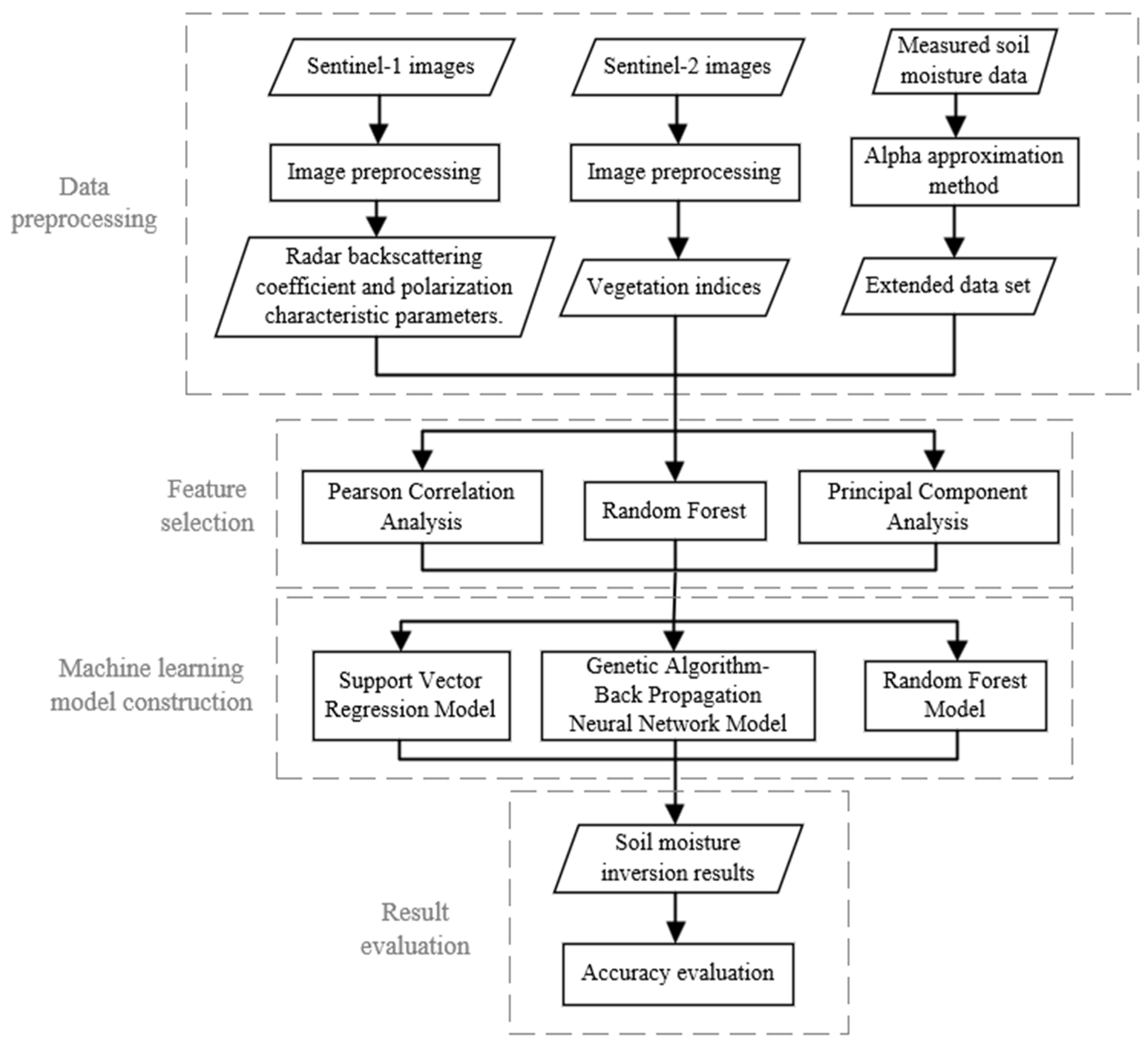
The technical roadmap of the proposed method is shown in
Figure 2.
The first step was data augmentation. The alpha approximation method was used to increase the sample size.
The second step was feature extraction. To obtain the necessary characteristic parameters, Sentinel-1 SAR data were preprocessed and H/A/αpolarization decomposition was carried out. The band data were extracted from the Sentinel-2 optical data, and the corresponding vegetation indices were calculated as the characteristic parameters.
The third step was feature optimization. The extracted feature parameters were optimized using 3 methods separately, including Pearson correlation analysis, RF, and PCA. The most advantageous feature subset was chosen based on the correlation between the characteristic parameters and the field-measured SSM values.
The fourth step was model building. To guarantee the training and inversion correctness of the models, GA-BP, SVR, and RF models were built and tweaked individually.
The fifth step was accuracy assessment. The inversion accuracy of 9 combinations of feature optimization methods and machine learning models was evaluated, and the optimal combination was chosen to retrieve the regional SSM of the study area.
2.2.1. Data Augmentation
For the problem of SSM inversion accuracy affected by the small size of the field measured SSM sample data, the alpha approximation method was adopted in this study to expand the sample size.
The alpha approximation method was proposed by Balenzano et al. [
23]. Assuming that vegetation conditions and surface roughness remain constant throughout time, the change in backscattering is only affected by changes in soil moisture [
25]. The quantitative link between backscattering coefficients and SSM is defined as Equations (1)–(3).
where
is the backscattering coefficient at time
i,
is the incidence angle,
is the soil dielectric constant,
is the polarization (
or
), and
is a function of the soil dielectric constant and the incident angle.
Equation (1) can be written as Equation (4).
When
N successive SAR image scenes are employed, the
N − 1 equations are summarized as Equation (5).
Equation (5) can be expressed as Equation (6) when three SAR image scenes are available.
where
and
can be acquired from the 3 Sentinel-1imgaes that are currently accessible. This indicates that there are 3 unknown parameters (specifically
) that need to be determined. After obtaining
as a prior information through ground estimates,
and
can be acquired using Equation (6).
Because the premise of this study was that vegetation conditions and surface roughness remain intact in a short period of time, Sentinel-1A data with a repetition period of 12 days is suitable for the experiment. In this paper, a field survey was carried out on 23 September 2021, the same day when Sentinel-1 satellite transited over the study area. When the other two Sentinel-1 scenarios are known and taken as previous knowledge, the SSM data on 11 September 2021, and 5 October 2021, can be simply inversed using the empirical expression of Equation (6).
In the field survey, 41 measured SSM samples were obtained. In the subsequent experiment, the measured samples were randomly split into two sets, which were the training set with 26 samples and the testing set with 15 samples. Only the training set was expanded using the alpha approximation method. The testing set remained unchanged and was utilized to assess the experimental accuracy. A total of 93 sampling points were obtained after data augmentation. To get rid of the interference, any outliers that may be present in the expanded data were removed.
2.2.2. Feature Parameter Extraction
The training accuracy of a machine learning model is highly connected to the number and quality of the training data. The model will converge too slowly if there is too much training data. This can impair the model’s ability to train on its own, lead to incorrect predictions, and lower the model’s accuracy. The prediction accuracy of the machine learning model can be increased while reducing consumption by analyzing the feature parameter set and choosing the feature parameters with strong correlation as the input data.
SAR works by sending microwave beams to objects and picking up echoes from those items to identify distinguishing traits. Radar information is directly impacted by both object characteristics and radar parameters, including the target object’s physical characteristics and the wavelength, incidence angle, and polarization mode [
28].
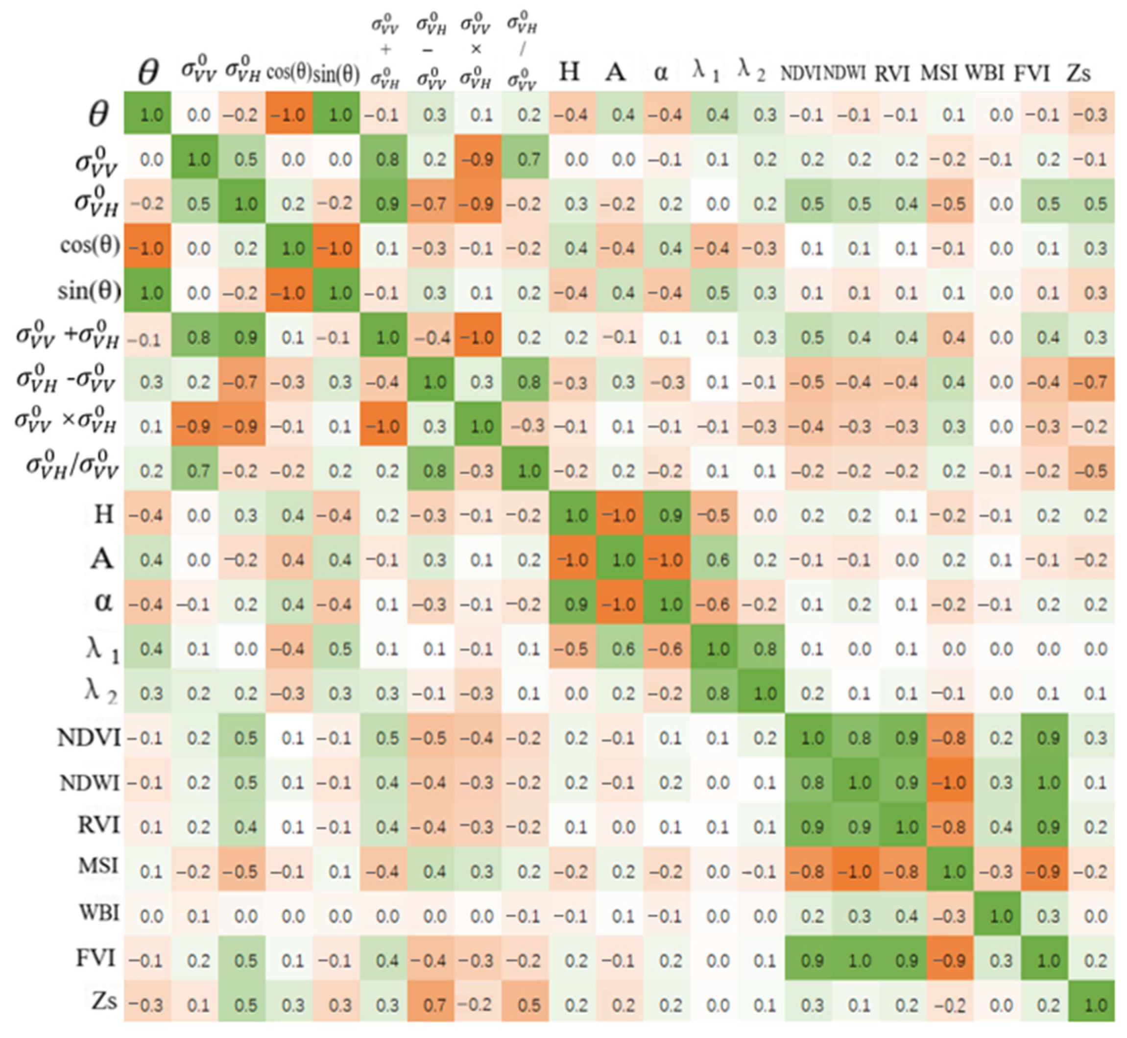
The incident angle (θ), VV, and VH polarization backscattering coefficients were extracted from the preprocessed Sentinel-1 SAR data and used as the defining parameters of the following experiments based on the latitude and longitude of each sampling point.
Both
cos(
θ) and
sin(
θ) are connected to soil moisture [
29]. The correlation between the backscattering coefficient and
sin(
θ) is larger in soils with higher soil moisture levels, and the correlation between the backscattering coefficient and
cos(
θ) is higher in soils with lower soil moisture levels. When the incident angle is constant, the backscattering coefficient increases with the increase of volumetric soil moisture content, and the combination of different polarization backscattering coefficients of (
+
), (
−
), (
×
) and (
/
) are also increased. More characteristic parameters from SAR remote sensing data can be extracted using polarization decomposition. H/A/α decomposition is used for eigenvalue decomposition of coherent matrix or covariance matrix of target features on Sentinel-1 dual polarization data, from which scattering entropy (
H), inverse entropy (
A), average scattering angle (
α) and eigenvalues (
λ1 and
λ2) can be extracted [
30].
Many vegetation indices can be generated from optical remote sensing data to describe surface vegetation information [
28]. The backscattering coefficient of SAR is not only related to its own polarization mode, incidence angle, and SSM, but also to the vegetation coverage and roughness of the surface. It is necessary for SSM inversion to remove or weaken the impact of vegetation and surface roughness. The vegetation index is the combination of ground reflectivity in two or more wavelength bands to accentuate a certain feature or detail of plants. Varied vegetation indices have different band application ranges and fields due to sensor kinds and band combinations.
According to the multi-band data provided by the multispectral imager (MSI) carried by Sentinel-2 and the actual vegetation coverage in the study area, six vegetation indices commonly used in SSM inversion research, including normalized difference vegetation index (NDVI), normalized difference moisture index (NDWI), specific vegetation index (RVI), water stress index (MSI), water body index (WBI) and fused vegetation index (FVI) [
31], were finally selected for this study. Their calculation formulas are shown in Equations (7)–(12).
where
490,
665,
842,
865,
945 and
1610 represent the band values corresponding to 490, 665, 842, 865, 945, 1610 nm in Sentinel-2 data, respectively. The 490 nm and 665 nm bands represent the blue and red of visible light. The 842 nm and 865 nm bands represent Near Infrared (NIR) and Narrow NIR. The 945 nm band represents water vapor. The 1610 nm band represents Short Wave Infrared (SWIR).
The surface roughness of the soil influences the microwave backscattering coefficient. The surface roughness information changes depending on the band frequency, incident angle, and polarization mode. Removing the influence of surface roughness on SSM inversion can increase accuracy. The surface combined roughness
Zs [
32] used in this study was calculated using SAR data and represented by Equations (13)–(15).
where
Av and
Bv are coefficients only applicable to the combined roughness model using C-band data, and only change with incident angle.
A total of 21 feature parameters were extracted from Sentinel-1 and Sentinel-2 data, as shown in
Table 2.
2.2.3. Feature Parameter Optimization
In this study, the extracted feature parameters were evaluated using Pearson correlation analysis, RF, and PCA methods separately to select the suitable feature parameter subset for the subsequent machine learning models.
The Pearson correlation coefficient, which has a value between −1 and 1, is the simplest approach to determine whether two variables are linearly connected. The sign indicates the positive-negative correlation. The closer its absolute value is to 1, the stronger the linear association between the two variables is. Conversely, the closer it is to 0, the weaker the linear relationship between the two variables is. It is calculated using Equation (16).
where
Cov (
X,
Y) represents the covariance of two variables
X and
Y,
Var(
X) is the variance of
X, and
Var(
Y) is the variance of
Y.
The RF method can calculate the relevance of each variable during the model-building process [
33]. In feature selection process with RF, the importance of each feature is first calculated and arranged in descending order. The proportion to be deleted is then established, and the matching proportion of characteristics is eliminated based on their relevance, yielding a new feature set. The preceding procedure with a new feature set is repeated until only m features remained, among which m is a preset value. Finally, the feature set with the lowest error rate is chosen based on each feature set acquired in the preceding process and its related error rate.
PCA is a method for finding a way to minimize the dimension of data while minimizing information loss [
34]. It is an important tool in data analysis and frequently used in machine learning to minimize the dimension of high-dimensional data, since it can extract the key characteristic variables from the data. Each vector has a correlation in high-dimensional data sets, whereas it has a linear independence in low-dimensional data sets, allowing the overlapping information in high-dimensional data sets to be removed [
35]. High-dimensional data are reduced to fulfill the goals of data dimensionality reduction, compression, and noise reduction. The data dimensionality is reduced, but the most relevant information is maintained, and certain unimportant aspects are deleted.
2.2.4. Construction of Machine Learning Models
Machine learning excels in nonlinear fitting. It is useful in resolving issues with excessive factors and convoluted structures in SSM inversion models. Even after sample augmentation, the number of samples is still limited due to the small number of field-measured SSM samples. Three field-measured typical machine learning models, GA-BP, SVR, and RF, that are appropriate for small sample training, were chosen for the study in order to prevent over-fitting.
Both neural networks and evolutionary algorithms are ways for imitating biological treatment modes and obtaining practical answers to complicated issues. The BP neural network is capable of adaptive learning and powerful nonlinear simulation. However, it is prone to local minima. In addition, the network’s design is not theoretically guided and is instead dependent on the designers’ expertise and repeated experimentation in the sample space, which restricts the network’s ability to find the overall optimal solution. GA can converge to the global optimal solution and has strong stability, but it lacks adaptive learning capabilities. As a result, combining a neural network with the genetic algorithm can enhance not only the neural network’s ability to generalize mapping, but also its rate of convergence, capacity for global optimization, and learning capacity [
36]. The entire prediction model is extensively upgraded in terms of accuracy and fitting capacity.
SVR is a regression analysis technique that uses the support vector machine (SVM). The majority of the sample points are situated outside the two decision boundaries thanks to the separation hyperplane that SVM discovers by maximizing the interval. In contrast to SVM, SVR also takes into account the maximum interval, but it also takes into account the points within the decision boundary to ensure that the majority of the sample points are situated within the interval. The most significant advantage of SVR is that it uses the kernel function rather than the inner product operation in high-dimensional space, transforming a high-dimensional nonlinear regression problem into a two-dimensional linear regression problem [
37].
RF can be used not only for parameter optimization, but also for parameter inversion. It is an integrated algorithm based on decision trees, with each decision tree acting as a classifier. When decision trees are being trained, randomness is incorporated, and samples and features are chosen at random. There will be n trees with n classification outcomes for each input sample. All the RF-categorized voting results are combined and the one with the most votes is chosen as the final result. In this process, integration and randomness coexist. RF model has the advantages of increasing prediction accuracy, decreasing over-fitting, and being unaffected by missing data and multi-collinearity [
38]. One advantage of RF is that it has good generalization performance due to the use of multiple regression trees, which helps to reduce model variability. It simply has two parameters, the number of trees and the number of features, therefore it doesn’t require complicated parameter adjustment [
17].
4. Discussion
4.1. Data Augmentation
Field measurements are necessary for soil moisture inversion. In practice, there are two main methods of field measuring. One is the traditional manual measuring method based on manual ground sampling and measurement on the date of satellite transits [
1,
4,
6,
8,
12,
13,
14,
15,
16,
17,
18,
19,
20,
22,
25,
26,
31,
33,
36,
38]. The other is the automatic measuring method based on ground-based observation stations or networks in the study area [
2,
3,
7,
21,
23,
24,
29]. Compared with the automatic measuring method, the field measured SSM data obtained through the traditional manual measuring method are often more difficult to collect, and usually in a limited number of times and in small quantities.
For those areas without any ground-based observation sites or automatic observation networks, like the study area in this paper, due to the limitations of time and space, the data obtained by manual field measurement are generally limited. The small size of field measured SSM data have a negative effect on SSM inversion accuracy, since there is insufficient data to train the inversion model and make a meaningful evaluation on the inversion results.
The experimental results shown in
Table 3 and
Table 6 demonstrated that, the proposed inversion method based on data augmentation was effective to supply more sample data for SSM inversion and further improved the inversion accuracy, providing a feasible reference for SSM inversion studies based on small sample size of field measured data.
It is worth noting that, the alpha approximation method used in this paper for data augmentation has a certain precondition, which assumed that the vegetation conditions and surface roughness remain unchanged in the short spanned period. So, the proposed method in this paper is not suitable for SSM inversion in those areas with large changes in the vegetation conditions and surface roughness in the study period. In fact, even in a short period, this precondition is difficult to strictly meet. In this study, although the dates of 11 September 2021 and 5 October 2021 were close to the middle date of 23 September 2021, and the vegetation conditions and surface roughness kept constant on the whole according to the field survey and actual situation, small changes in some parts of the study area were ineluctable. This fact affected the application of the alpha approximation method and further the SSM inversion accuracy of the proposed method. In the future, more reliable and effective data augmentation methods will be explored to expand the sample size, thus to further improving the SSM inversion accuracy.
4.2. Accuracy Analysis
After data augmentation, the parameters extracted from remote sensing data and machine learning models for SSM inversion were optimized to improve the SSM inversion accuracy further.
Three parameter optimization methods, which were Pearson correlation analysis, RF and PCA, were proven to be effective for parameter optimization in SSM inversion [
22,
34,
38], and so chosen in this study to reduce the redundant features and improve the accuracy of model estimation. The experimental results shown in
Table 4 and
Table 5 and
Figure 3 indicated that, it was hard to get a uniform optimal feature subset through these three different optimization methods, due to their different optimization principles and evaluation criteria. Inspired by the research in reference [
22], the extracted parameters and the used inversion models were optimized in the whole in this study by using different combinations of parameter optimization methods and machine learning models. In order to ensure the homogeneity of the experiments, the first eight features in each ranking result of the feature optimization method were uniformly selected as the ideal feature subset for the subsequent experiments. However, it was not ensured that the subsets with the first eight features for all these three methods could all reach the final maximum inversion accuracy for all these nine model combinations. Different sizes of optimal feature subsets for different feature selection methods may be more reasonable for the proposed method and will be explored in this study to further improve the SSM inversion accuracy.
Three typical machine learning models commonly used in SSM inversion, which were GA-BP [
36,
38], SVR [
15,
18,
19,
26,
33], and RF [
16,
23,
33,
34,
38], were selected in this study because of their good performance in SSM inversion based on the small size of samples [
15,
16,
19,
33,
36,
38]. Combined with three parameter optimization methods, the performance of nine different model combinations in SSM inversion was compared in the experiments. According to the experimental results shown in
Table 6, the combination of employing RF for feature selection and RF for SSM inversion offered the maximum inversion accuracy, with higher R
2 and lower RSME and MAE than other combinations.
The performance of GA-BP and SVR models was a little worse than that of the RF model in this study, although they are generally considered to have good generalization ability when the sample size is small. One possible reason is that some parameters of GA-BP and SVR models may be not set properly and could be further optimized. Another possible reason is that there was an over-fitting issue in their training process because the sample size in this study was too small, which also affected the performance of the RF model in this study.
A total of 41 measured SSM samples were obtained in the field survey, and expanded to 93 samples after data augmentation. Compared with the original sample data and previous SSM inversion studies based on small samples [
1,
4,
6,
15,
16,
18,
19,
33,
36,
38], the sample size had increased. However, due to the limited initial sample size and the limitations of the alpha approximation method, the sample size was still limited, which was prone to over-fitting issues in practice. A considerable sample set is still the guarantee for sufficient model training and reasonable inversion accuracy. More field measurements are planned in this study in the future.
Even though, for those SSM inversion studies based on a small sample size of field measured data, as demonstrated in this study, the data augmentation method was still an effective way to supply more sample data and further improved the inversion accuracy.

 ,
, 


