
Potential for Peatland Water Table Depth Monitoring Using Sentinel-1 SAR Backscatter: Case Study of Forsinard Flows, Scotland, UK

 , , , , ,
Abstract
:1. Introduction
- Investigate the correlation between Sentinel-1 radar data and WTD in blanket bogs in the Flow Country of northern Scotland, ranging from intact and near-natural sites to sites damaged by past afforestation and drainage, where restoration has recently started.
- Create and test models with different complexities for WTD estimation using Sentinel-1 data.
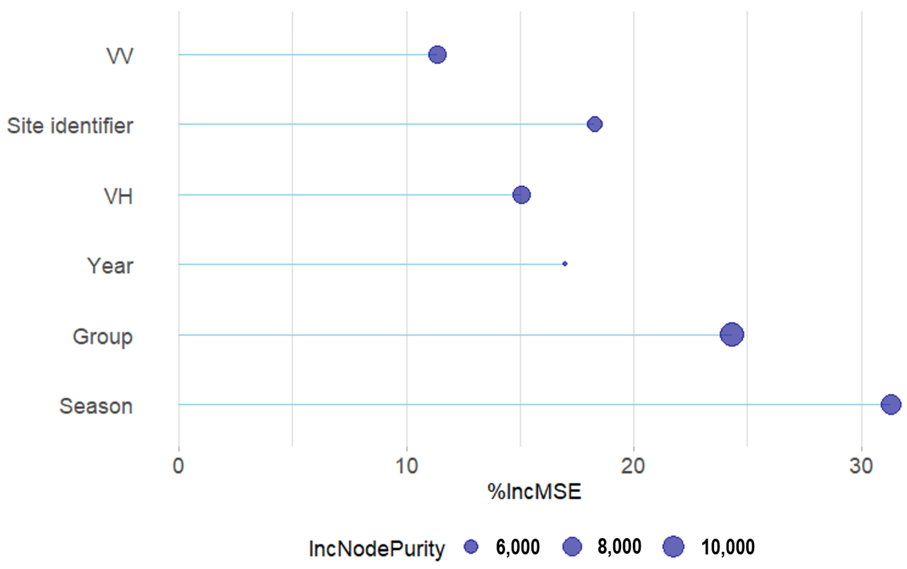
- Characterise the effects of surface roughness, hydrological condition (characterized by WTD measurements), seasonality, and time of acquisition in the developed models.
2. Materials and Methods
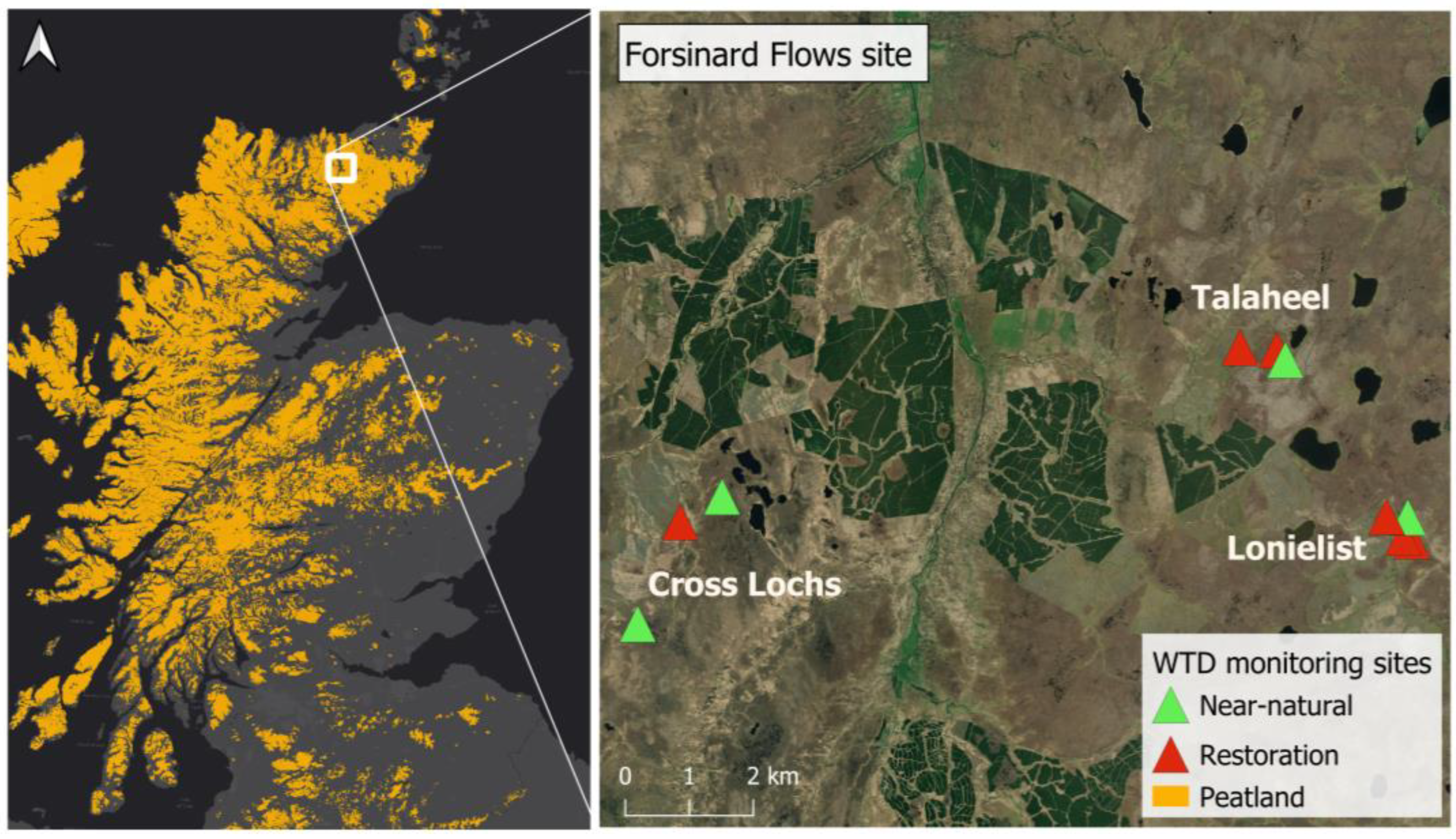
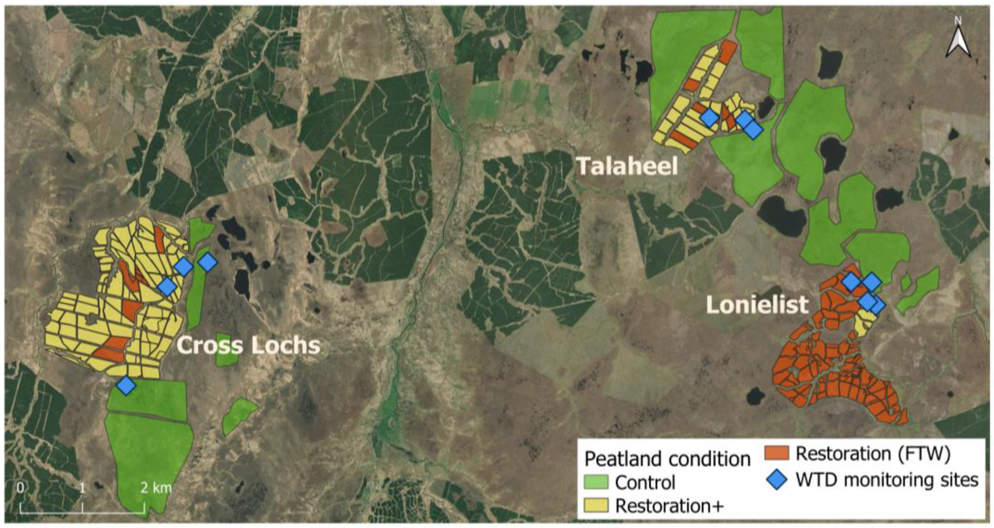
2.1. Study Area
2.2. Water Table Depth and Meteorological Data
2.3. Remotely Sensed Data
2.4. LiDAR Data and TRI Analysis
2.5. Model Generation and Statistical Analysis
3. Results
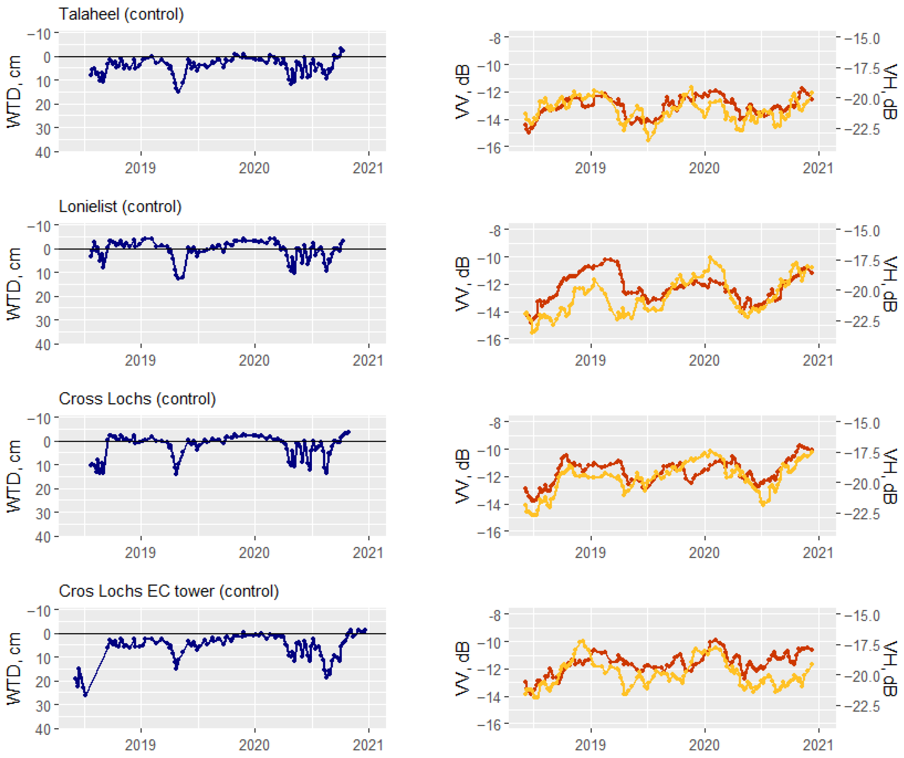
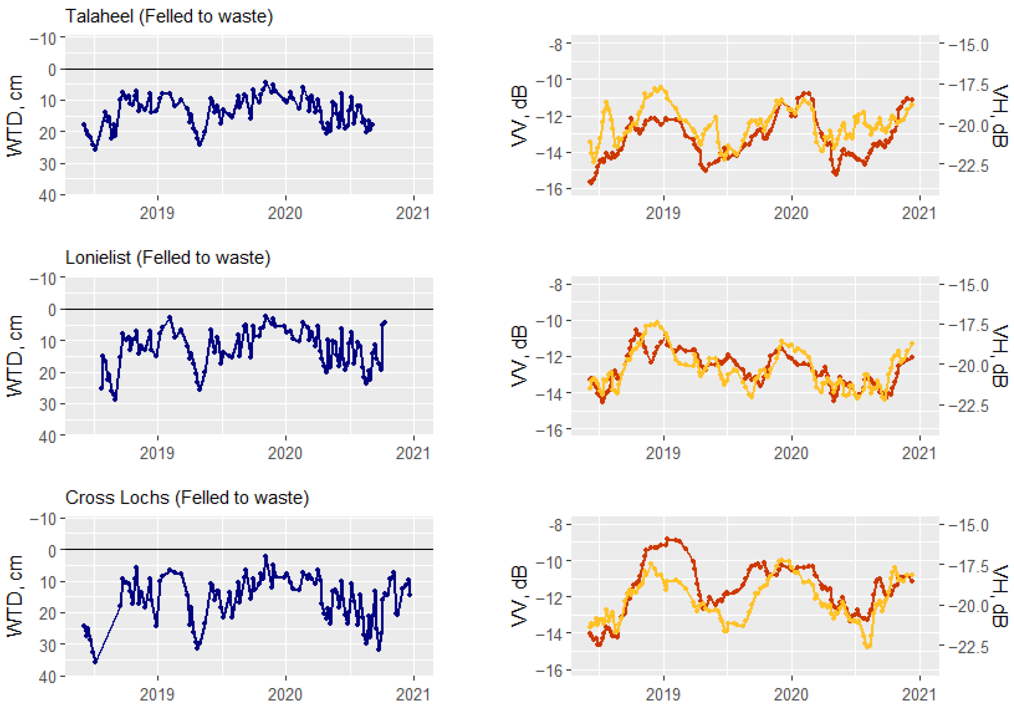
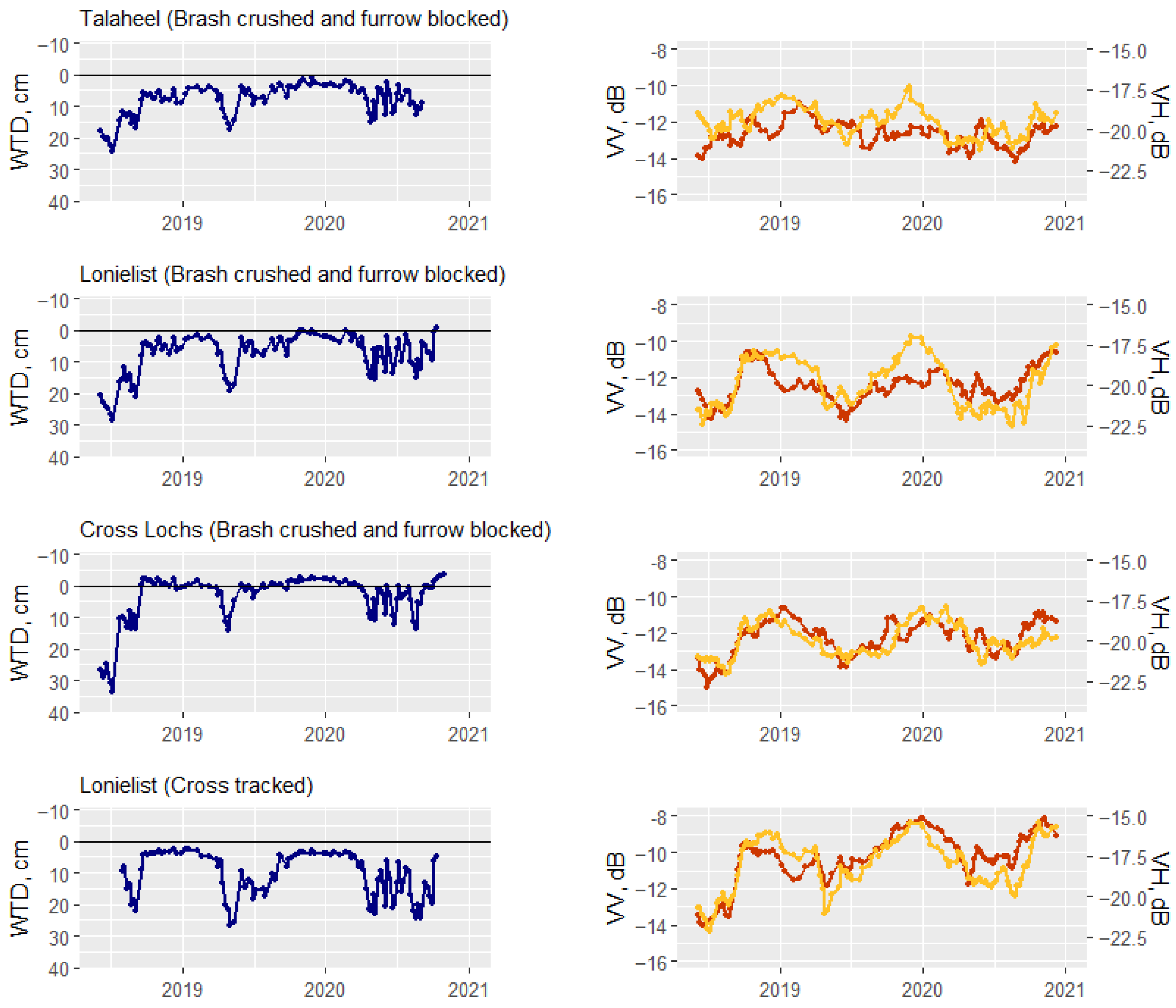
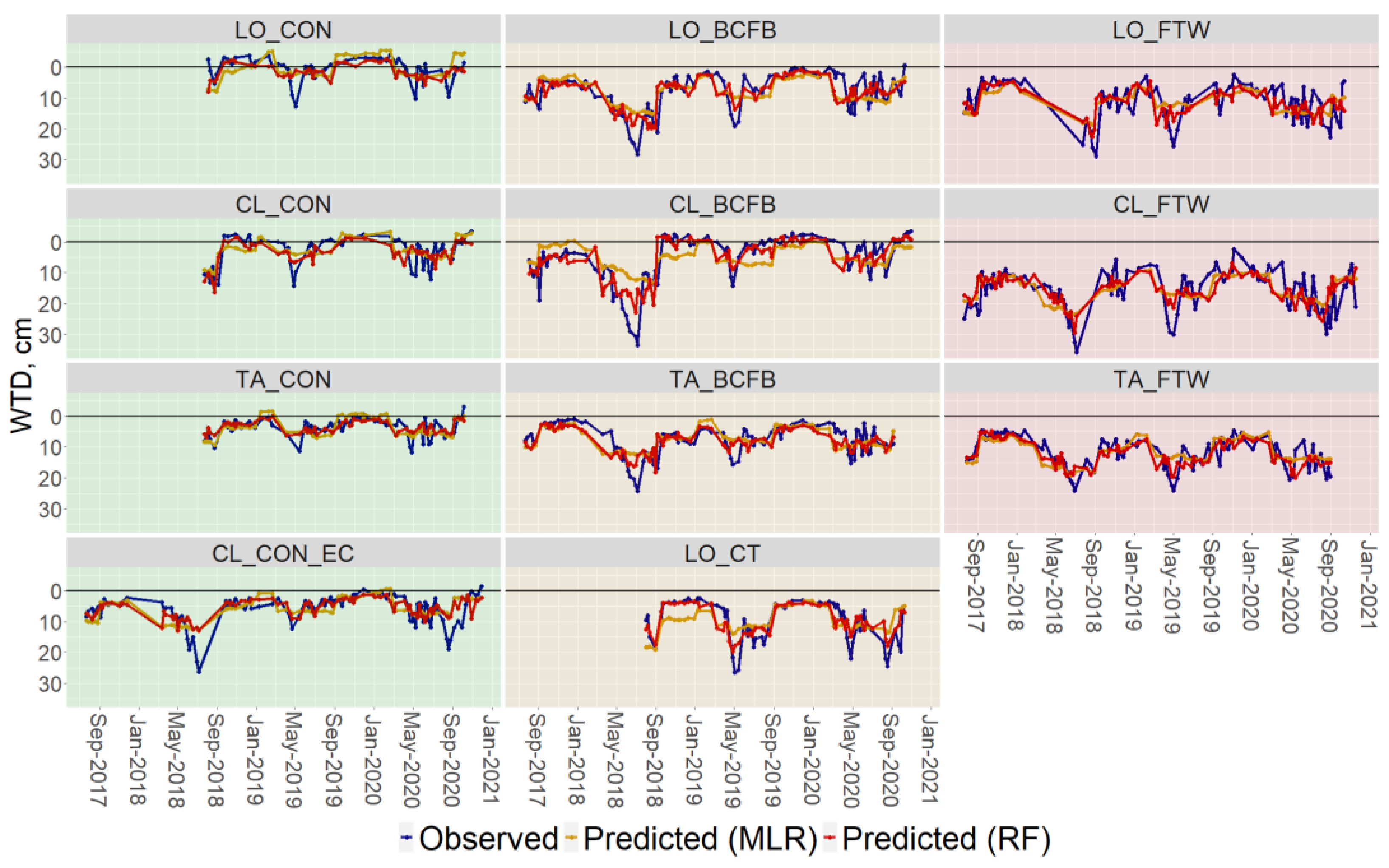
3.1. Water Table Depth and Sentinel-1 Time Series Analysis
3.1.1. Near-Natural Peatlands—Control Areas
3.1.2. Restoration—Felled to Waste
3.1.3. Restoration with Additional Management
3.2. Correlation of Sentinel-1 Backscatter and Water Table Depth
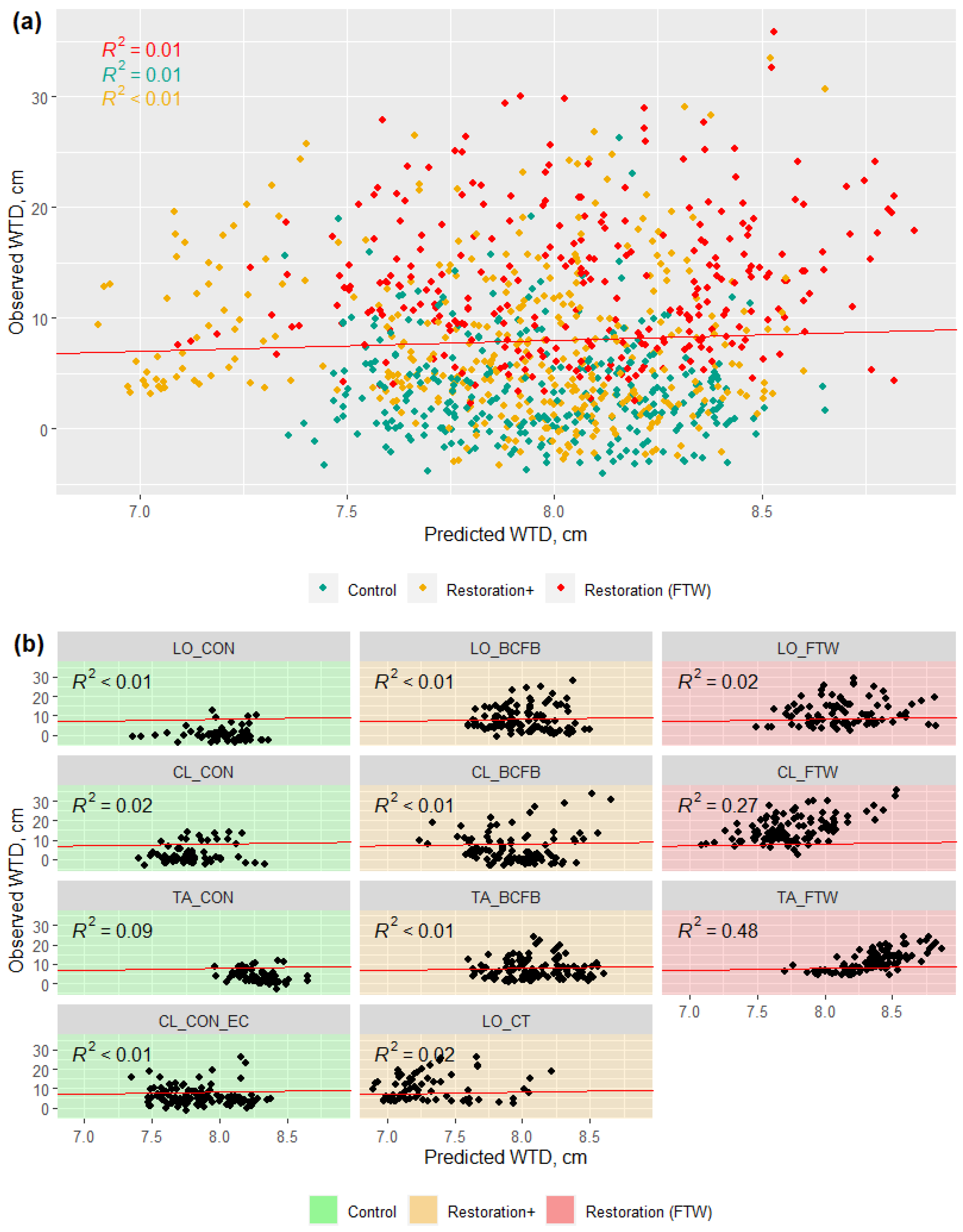
3.2.1. SLR Model
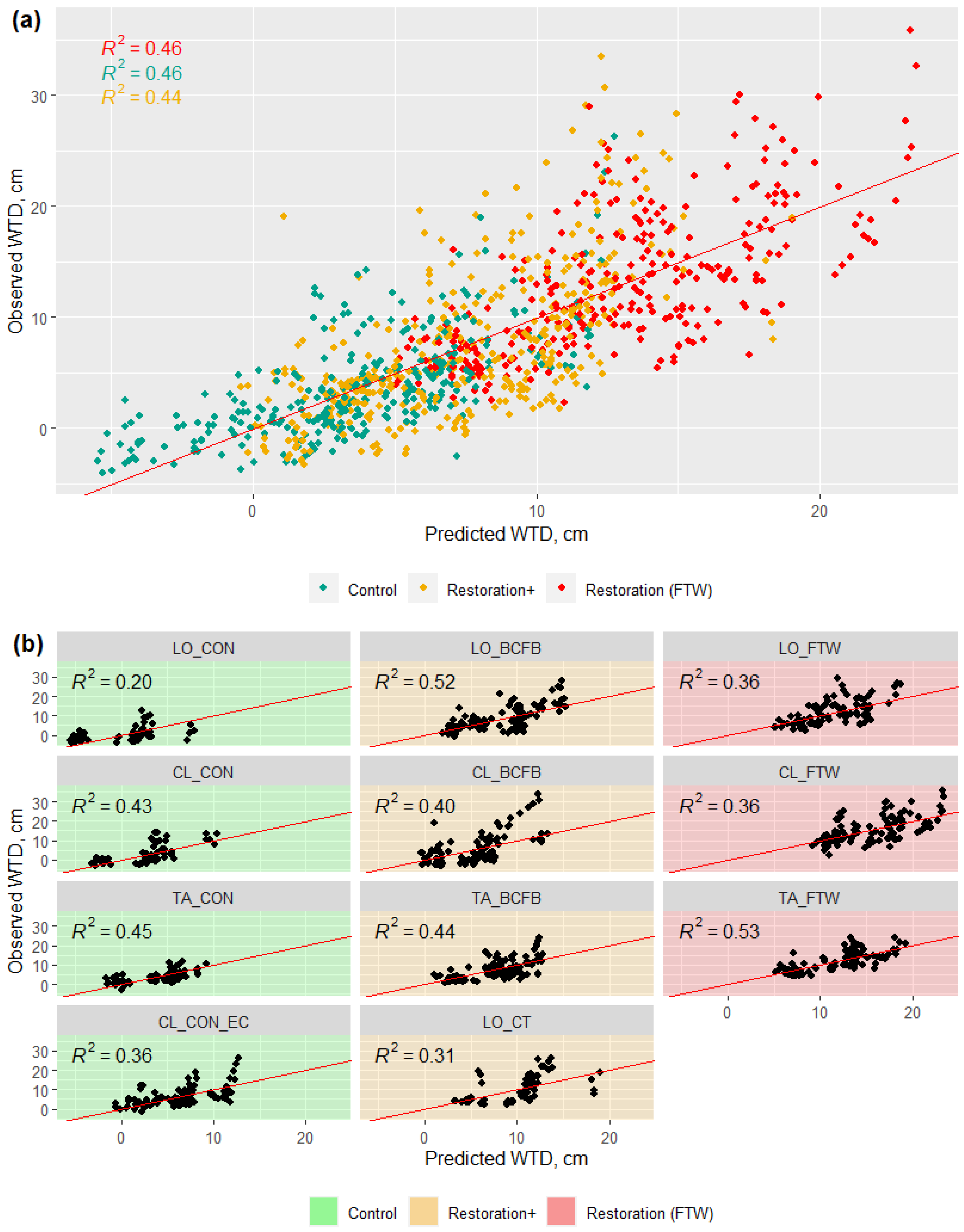
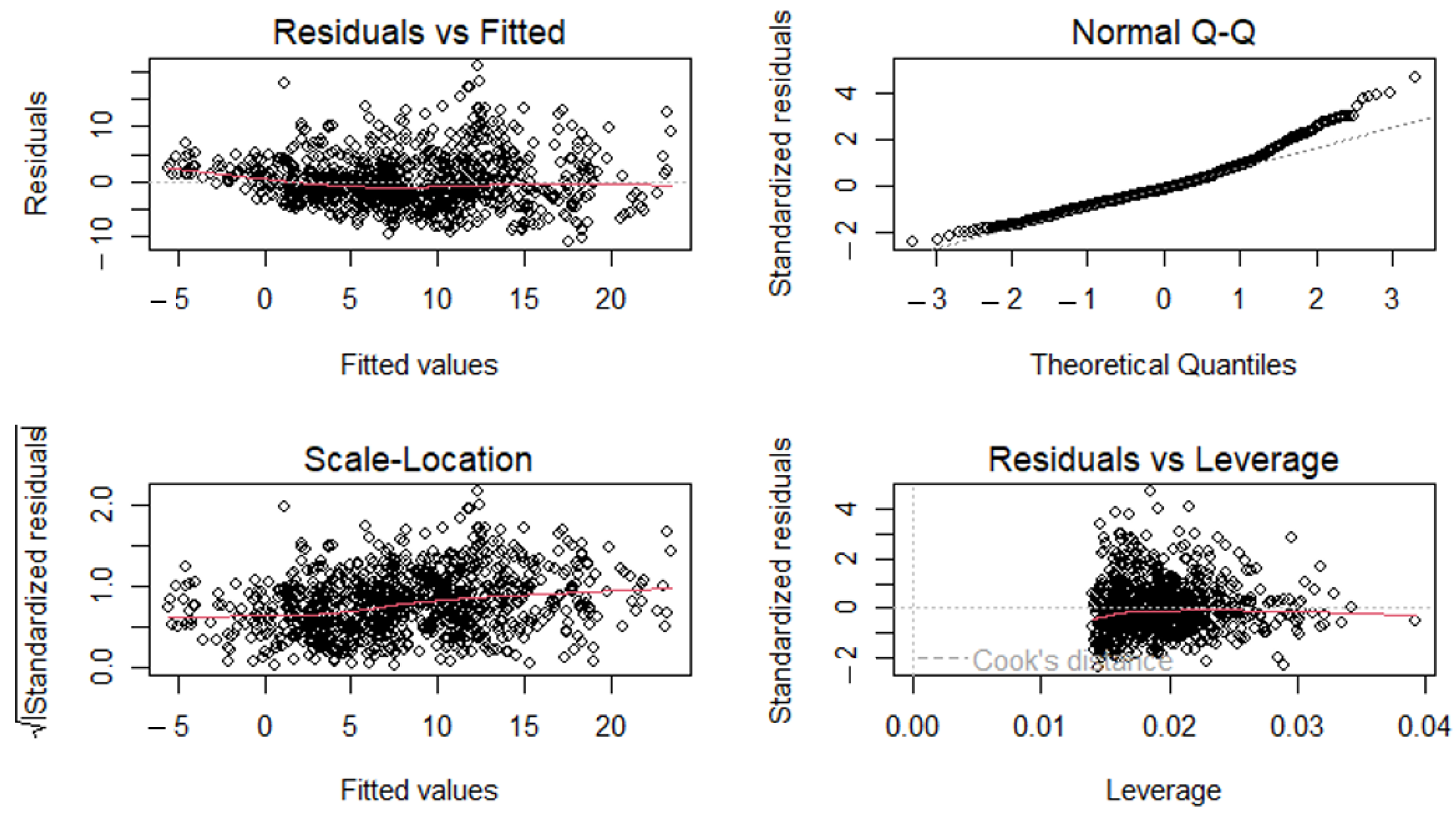
3.2.2. MLR Model
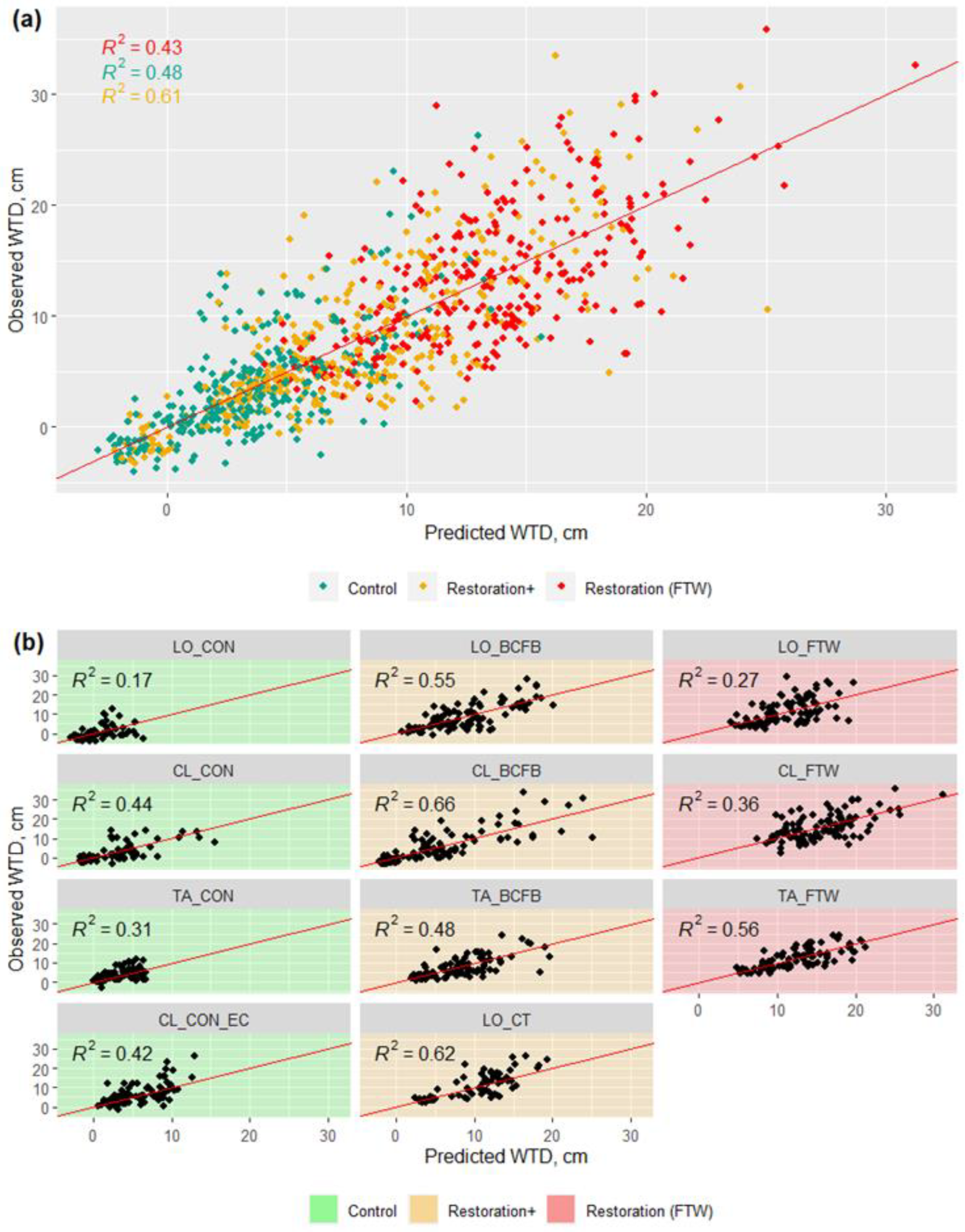
3.2.3. RF Model
4. Discussion
- Topography and microtopography: gullies, hags, hummocks, hollows, pools, ridge and furrow pattern;
- Soil and vegetation moisture content, inundation;
- Varying vegetation;
- Soil density and texture.
5. Conclusions
Supplementary Materials
Author Contributions
Funding
Data Availability Statement
Acknowledgments
Conflicts of Interest
References
- Lindsay, R.A.; Charman, D.J.; Everingham, F.; Reilly, R.M.O.; Palmer, M.A.; Rowell, T.A.; Stroud, D.A.; Ratcliffe, D.A.; Oswald, P.H.; O’Reilly, R.M.; et al. Part I Peatland Ecology. The Flow Country—The Peatlands of Caithness and Sutherland; Joint Nature Conservation Committee: Peterborough, UK, 1988. [Google Scholar]
- Gallego-Sala, A.V.; Colin Prentice, I. Blanket Peat Biome Endangered by Climate Change. Nat. Clim. Chang. 2013, 3, 152–155. [Google Scholar] [CrossRef]
- Joosten, H.; Tapio-Biström, M.-L.; Tol, S. Peatlands—Guidance for Climate Change Mitigation through Conservation, Rehabilitation and Sustainable Use; Joint Nature Conservation Committee: Peterborough, UK, 2012. [Google Scholar]
- Alderson, D.M.; Evans, M.G.; Shuttleworth, E.L.; Pilkington, M.; Spencer, T.; Walker, J.; Allott, T.E.H. Trajectories of Ecosystem Change in Restored Blanket Peatlands. Sci. Total Environ. 2019, 665, 785–796. [Google Scholar] [CrossRef]
- Sottocornola, M.; Boudreau, S.; Rochefort, L. Peat Bog Restoration: Effect of Phosphorus on Plant Re-Establishment. Ecol. Eng. 2007, 31, 29–40. [Google Scholar] [CrossRef]
- Lucchese, M.; Waddington, J.M.; Poulin, M.; Pouliot, R.; Rochefort, L.; Strack, M. Organic Matter Accumulation in a Restored Peatland: Evaluating Restoration Success. Ecol. Eng. 2010, 36, 482–488. [Google Scholar] [CrossRef]
- Hancock, M.H.; Klein, D.; Andersen, R.; Cowie, N.R. Vegetation Response to Restoration Management of a Blanket Bog Damaged by Drainage and Afforestation. Appl. Veg. Sci. 2018, 21, 167–178. [Google Scholar] [CrossRef]
- Kalacska, M.; Arroyo-Mora, J.P.; Soffer, R.J.; Roulet, N.T.; Moore, T.R.; Humphreys, E.; Leblanc, G.; Lucanus, O.; Inamdar, D. Estimating Peatland Water Table Depth and Net Ecosystem Exchange: A Comparison between Satellite and Airborne Imagery. Remote Sens. 2018, 10, 687. [Google Scholar] [CrossRef]
- Evans, C.D.; Peacock, M.; Baird, A.J.; Artz, R.R.E.; Burden, A.; Callaghan, N.; Chapman, P.J.; Cooper, H.M.; Coyle, M.; Craig, E.; et al. Overriding Water Table Control on Managed Peatland Greenhouse Gas Emissions. Nature 2021, 1, 65. [Google Scholar] [CrossRef] [PubMed]
- Czapiewski, S.; Szumińska, D. An Overview of Remote Sensing Data Applications in Peatland Research Based on Works from the Period 2010–2021. Land 2022, 11, 24. [Google Scholar] [CrossRef]
- Luscombe, D.J.; Anderson, K.; Gatis, N.; Grand-Clement, E.; Brazier, R.E. Using Airborne Thermal Imaging Data to Measure Near-Surface Hydrology in Upland Ecosystems. Hydrol. Process. 2015, 29, 1656–1668. [Google Scholar] [CrossRef]
- Bradley, A.V.; Andersen, R.; Marshall, C.; Sowter, A.; Large, D.J. Identification of Typical Ecohydrological Behaviours Using InSAR Allows Landscape-Scale Mapping of Peatland Condition. Earth Surf. Dyn. 2022, 10, 261–277. [Google Scholar] [CrossRef]
- Alshammari, L.; Boyd, D.S.; Sowter, A.; Marshall, C.; Andersen, R.; Gilbert, P.; Marsh, S.; Large, D.J. Use of Surface Motion Characteristics Determined by InSAR to Assess Peatland Condition. J. Geophys. Res. Biogeosci. 2020, 125, e2018JG004953. [Google Scholar] [CrossRef]
- Klinke, R.; Kuechly, H.; Frick, A.; Förster, M.; Schmidt, T.; Holtgrave, A.-K.; Kleinschmit, B.; Spengler, D.; Neumann, C. Indicator-Based Soil Moisture Monitoring of Wetlands by Utilizing Sentinel and Landsat Remote Sensing Data. PFG-J. Photogramm. Remote Sens. Geoinf. Sci. 2018, 86, 71–84. [Google Scholar] [CrossRef]
- Bechtold, M.; Schlaffer, S.; Tiemeyer, B.; Lannoy, G. de Inferring Water Table Depth Dynamics from ENVISAT-ASAR C-Band Backscatter over a Range of Peatlands from Deeply-Drained to Natural Conditions. Remote Sens. 2018, 10, 536. [Google Scholar] [CrossRef]
- Kim, J.W.; Lu, Z.; Gutenberg, L.; Zhu, Z. Characterizing Hydrologic Changes of the Great Dismal Swamp Using SAR/InSAR. Remote Sens. Environ. 2017, 198, 187–202. [Google Scholar] [CrossRef]
- Asmuß, T.; Bechtold, M.; Tiemeyer, B. On the Potential of Sentinel-1 for High Resolution Monitoring of Water Table Dynamics in Grasslands on Organic Soils. Remote Sens. 2019, 11, 1659. [Google Scholar] [CrossRef]
- Toca, L.; Morrison, K.; Artz, R.R.E.; Gimona, A.; Quaife, T. High Resolution C-Band SAR Backscatter Response to Peatland Water Table Depth and Soil Moisture: A Laboratory Experiment. Int. J. Remote Sens. 2022, 43, 5231–5251. [Google Scholar] [CrossRef]
- Bourgeau-Chavez, L.L.; Smith, K.B.; Brunzell, S.M.; Kasischke, E.S.; Romanowicz, E.A.; Richardson, C.J. Remote Monitoring of Regional Inundation Patterns and Hydroperiod in the Greater Everglades Using Synthetic Aperture Radar. Wetlands 2005, 25, 176–191. [Google Scholar] [CrossRef]
- Millard, K.; Richardson, M. Quantifying the Relative Contributions of Vegetation and Soil Moisture Conditions to Polarimetric C-Band SAR Response in a Temperate Peatland. Remote Sens. Environ. 2018, 206, 123–138. [Google Scholar] [CrossRef]
- Torbick, N.; Persson, A.; Olefeldt, D.; Frolking, S.; Salas, W.; Hagen, S.; Crill, P.; Li, C. High Resolution Mapping of Peatland Hydroperiod at a High-Latitude Swedish Mire. Remote Sens. 2012, 4, 974. [Google Scholar] [CrossRef]
- Räsänen, A.; Tolvanen, A.; Kareksela, S. Monitoring Peatland Water Table Depth with Optical and Radar Satellite Imagery. Int. J. Appl. Earth Obs. Geoinf. 2022, 112, 102866. [Google Scholar] [CrossRef]
- Aitkenhead, M.; Coull, M. Mapping Soil Profile Depth, Bulk Density and Carbon Stock in Scotland Using Remote Sensing and Spatial Covariates. Eur. J. Soil Sci. 2020, 71, 553–567. [Google Scholar] [CrossRef]
- Artz, R.; Faccioli, M.; Roberts, M.; Anderson, R. Peatland Restoration—A Comparative Analysis of the Costs and Merits of Different Restoration Methods. ClimateXChange 2018. [Google Scholar]
- Levy, P.E.; Gray, A. Greenhouse Gas Balance of a Semi-Natural Peatbog in Northern Scotland. Environ. Res. Lett. 2015, 10, 094019. [Google Scholar] [CrossRef]
- Artz, R.R.E.; Coyle, M.; Donaldson-Selby, G.; Morrison, R. Net Carbon Dioxide Emissions from an Eroding Atlantic Blanket Bog. Biogeochemistry 2022, 159, 233–250. [Google Scholar] [CrossRef]
- ESA Data Products. ESA: Sentinel-1 Data Products. Available online: https://sentinel.esa.int/web/sentinel/missions/sentinel-1/data-products (accessed on 17 August 2022).
- GEE GEE Guide. GEE Guide: Sentinel-1 Algorithms. Available online: https://developers.google.com/earth-engine/guides/sentinel1 (accessed on 5 August 2022).
- Benninga, H.J.F.; van der Velde, R.; Su, Z. Impacts of Radiometric Uncertainty and Weather-Related Surface Conditions on Soil Moisture Retrievals with Sentinel-1. Remote Sens. 2019, 11, 2025. [Google Scholar] [CrossRef]
- Shawn, R.; DeGloria, S.D.; Elliot, R. A Terrain Ruggedness Index That Quantifies Topographic Heterogeneity. Intermt. J. Sci. 1999, 5, 23–27. [Google Scholar]
- R Core Team R Core Team. R: A Language and Environment for Statistical Computing; R Foundation for Statistical Computing: Vienna, Austria, 2021; Available online: http://www.R-project.org (accessed on 1 September 2022).
- Kasischke, E.S.; Bourgeau-Chavez, L.L.; Rober, A.R.; Wyatt, K.H.; Waddington, J.M.; Turetsky, M.R. Effects of Soil Moisture and Water Depth on ERS SAR Backscatter Measurements from an Alaskan Wetland Complex. Remote Sens. Environ. 2009, 113, 1868–1873. [Google Scholar] [CrossRef]
- Liaw, A.; Wiener, M. Classification and Regression by RandomForest. R News 2002, 2, 18–22. [Google Scholar]
- Breiman, L. Random Forests. Mach Learn 2001, 45, 123–140. [Google Scholar] [CrossRef]
- Schuldt, B.; Buras, A.; Arend, M.; Vitasse, Y.; Beierkuhnlein, C.; Damm, A.; Gharun, M.; Grams, T.E.E.; Hauck, M.; Hajek, P.; et al. A First Assessment of the Impact of the Extreme 2018 Summer Drought on Central European Forests. Basic Appl. Ecol. 2020, 45, 86–103. [Google Scholar] [CrossRef]
- Dettmann, U.; Bechtold, M. Deriving Effective Soil Water Retention Characteristics from Shallow Water Table Fluctuations in Peatlands. Vadose Zone J. 2016, 15, 1–13. [Google Scholar] [CrossRef]
- Scholefield, P.; Morton, D.; McShane, G.; Carrasco, L.; Whitfield, M.G.; Rowland, C.; Rose, R.; Wood, C.; Tebbs, E.; Dodd, B.; et al. Estimating Habitat Extent and Carbon Loss from an Eroded Northern Blanket Bog Using UAV Derived Imagery and Topography. Prog. Phys. Geogr. 2019, 43, 282–298. [Google Scholar] [CrossRef]
- Holden, J.; Wallage, Z.E.; Lane, S.N.; McDonald, A.T. Water Table Dynamics in Undisturbed, Drained and Restored Blanket Peat. J. Hydrol. 2011, 402, 103–114. [Google Scholar] [CrossRef]
- Lees, K.J.; Artz, R.R.E.; Chandler, D.; Aspinall, T.; Boulton, C.A.; Buxton, J.; Cowie, N.R.; Lenton, T.M. Using Remote Sensing to Assess Peatland Resilience by Estimating Soil Surface Moisture and Drought Recovery. Sci. Total Environ. 2021, 761, 143312. [Google Scholar] [CrossRef]
- Mc Nairn, H.; Boisvert, J.B.; Major, D.J.; Gwyn, Q.H.J.; Brown, R.J.; Smith, A.M. Identification of Agricultural Tillage Practices from C-Band Radar Backscatter. Can. J. Remote Sens. 1996, 22, 154–162. [Google Scholar] [CrossRef]
- Küttim, M.; Küttim, L.; Ilomets, M.; Laine, A.M. Controls of Sphagnum Growth and the Role of Winter. Ecol. Res. 2020, 35, 219–234. [Google Scholar] [CrossRef]
- Maslanka, W.; Morrison, K.; White, K.; Verhoef, A.; Clark, J. Retrieval of Sub-Kilometric Relative Surface Soil Moisture With Sentinel-1 Utilizing Different Backscatter Normalization Factors. IEEE Trans. Geosci. Remote Sens. 2022, 60, 1–13. [Google Scholar] [CrossRef]
- Quaife, T.; Pinnington, E.M.; Marzahn, P.; Kaminski, T.; Vossbeck, M.; Timmermans, J.; Isola, C.; Rommen, B.; Loew, A. Synergistic Retrievals of Leaf Area Index and Soil Moisture from Sentinel-1 and Sentinel-2. Int. J. Image Data Fusion 2022, 1–18. [Google Scholar] [CrossRef]


| Near-Natural (Control) | Restoration (Felled to Waste) | Restoration+ (Felling and Additional Management) | |
|---|---|---|---|
| Aerial photograph (natural colour (RGB) orthophoto, 50 cm resolution, March 2017) |  |  |  |
| Terrain ruggedness index, TRI (cm) | 9.6 | 21.3 | 12.5 |
| Mean WTD * ± SD (cm) | 4.9 ± 3.5 | 12.3 ± 4.0 | 11.3 ± 5.4 |
| Year afforested | - | 1983 | 1985 |
| Year felled | - | 1998 | 1998 |
| Year of additional restoration management | - | - | 2016 |
| Restoration method | - | - | Brash-crushing and furrow-blocking |
| Abbreviation | TA_CON | TA_FTW | TA_BCFB |
| Near-Natural (Control) | Restoration (Felled to Waste) | Restoration+ (Felling and Additional Management) | |
|---|---|---|---|
| Aerial photograph (natural colour (RGB) orthophoto, 50 cm resolution, March 2017) |  |  | (a)  (b)  |
| Terrain ruggedness index, TRI (cm) | 9.7 | 16.8 | (a) 14.0 (b) 17.0 |
| Mean WTD * ± SD (cm) | 2.8 ± 3.8 | 12.9 ± 5.6 | (a) 3.8 ± 4.7 (b) 9.4 ± 7.0 |
| Year afforested | - | 1985 | 1985 |
| Year felled | - | 2006 | (a) 2006 (b) 2004 |
| Year of additional restoration management | - | - | (a) 2012, 2018 (b) - |
| Restoration method | - | - | (a) Brash-crushing and furrow-blocking (b) Cross-tracking and furrow-blocking |
| Abbreviation | LO_CON | LO_FTW | (a) LO_BCFB (b) LO_CT |
| Near-Natural (Control) | Restoration (Felled to Waste) | Restoration+ (Felling and Additional Management) | |
|---|---|---|---|
| Aerial photograph (natural colour (RGB) orthophoto, 50 cm resolution, March 2017) | (a)  (b)  |  |  |
| Terrain ruggedness index, TRI (cm) | (a) 3.8 (b) 3.2 | 5.0 | 2.8 |
| Mean WTD * ± SD (cm) | (a) 4.9 ± 4.7 (b) 0.9 ± 2.5 | 14.7 ± 7.0 | 4.9 ± 4.5 |
| Year afforested | - | 1983 | 1983 |
| Year felled | - | 2006 | 2005 |
| Year of additional restoration management | - | - | 2016 |
| Restoration method | - | - | Brash-crushing and furrow-blocking |
| Abbreviation | (a) CL_CON (b) CL_CON_EC | CL_FTW | CL_BCFB |
| Treatment | Site | Simple Linear Regression, SLR (R2) | Multiple Linear Regression MLR (R2) | Random Forest, RF (R2) | Terrain Ruggedness Index, TRI (cm) | Standing Water (%) | Forestry Ridge and Furrow Lines (Aspect, °) | |||
|---|---|---|---|---|---|---|---|---|---|---|
| Training | Validation | Training | Validation | Training | Validation | |||||
| Near-natural (Control) | TA_CON | 0.09 * | 0.02 | 0.45 *** | 0.26 ** | 0.30 *** | 0.25 ** | 9.6 | 2 | - |
| CL_CON | 0.02 | <0.01 | 0.43 *** | 0.52 *** | 0.45 *** | 0.61 *** | 3.8 | 5 | - | |
| LO_CON | <0.01 | 0.02 | 0.20 *** | 0.25 *** | 0.16 *** | 0.21 ** | 9.7 | 5 | - | |
| CL_CON_EC | <0.01 | 0.04 | 0.36 *** | 0.52 ** | 0.43 *** | 0.52 *** | 3.2 | 15 | - | |
| Control group | 0.01 | <0.01 | 0.46 *** | 0.50 *** | 0.48 *** | 0.50 *** | 6.6 | |||
| Restored (felled to waste) | TA_FTW | 0.48 *** | 0.09 | 0.53 *** | 0.16 ** | 0.56 *** | 0.14 * | 21.3 | 5 | −60° |
| CL_FTW | 0.27 *** | 0.08 | 0.36 *** | 0.19 ** | 0.36 *** | 0.18 ** | 5.0 | 5 | −26° | |
| LO_FTW | 0.02 | 0.04 | 0.36 *** | 0.61 *** | 0.29 *** | 0.35 *** | 16.8 | 20 | −17° | |
| Restoration (FTW) group | 0.01 | <0.01 | 0.46 *** | 0.34 *** | 0.44 *** | 0.26 *** | 14.4 | |||
| Restored with additional management | TA_BCFB | <0.01 | <0.01 | 0.44 *** | 0.21 ** | 0.53 *** | 0.06 | 12.5 | 45 | −16° |
| CL_BCFB | <0.01 | 0.02 | 0.40 *** | 0.36 *** | 0.63 *** | 0.39 *** | 2.8 | 45 | −22° | |
| LO_BCFB | <0.01 | <0.01 | 0.52 *** | 0.43 *** | 0.54 *** | 0.51 *** | 14.0 | 30 | −30° | |
| LO_CT | 0.02 | <0.01 | 0.31 *** | 0.41 *** | 0.66 *** | 0.38 *** | 17.0 | 5 | −57° | |
| Restoration+ Group | <0.01 | 0.04 | 0.44 *** | 0.44 *** | 0.61 *** | 0.40 *** | 11.6 | |||
| Combined | <0.01 | <0.01 | 0.59 *** | 0.62 *** | 0.66 *** | 0.60 *** | ||||
Disclaimer/Publisher’s Note: The statements, opinions and data contained in all publications are solely those of the individual author(s) and contributor(s) and not of MDPI and/or the editor(s). MDPI and/or the editor(s) disclaim responsibility for any injury to people or property resulting from any ideas, methods, instructions or products referred to in the content. |
© 2023 by the authors. Licensee MDPI, Basel, Switzerland. This article is an open access article distributed under the terms and conditions of the Creative Commons Attribution (CC BY) license (https://creativecommons.org/licenses/by/4.0/).
Share and Cite
Toca, L.; Artz, R.R.E.; Smart, C.; Quaife, T.; Morrison, K.; Gimona, A.; Hughes, R.; Hancock, M.H.; Klein, D. Potential for Peatland Water Table Depth Monitoring Using Sentinel-1 SAR Backscatter: Case Study of Forsinard Flows, Scotland, UK. Remote Sens. 2023, 15, 1900. https://doi.org/10.3390/rs15071900
Toca L, Artz RRE, Smart C, Quaife T, Morrison K, Gimona A, Hughes R, Hancock MH, Klein D. Potential for Peatland Water Table Depth Monitoring Using Sentinel-1 SAR Backscatter: Case Study of Forsinard Flows, Scotland, UK. Remote Sensing. 2023; 15(7):1900. https://doi.org/10.3390/rs15071900
Chicago/Turabian StyleToca, Linda, Rebekka R. E. Artz, Catherine Smart, Tristan Quaife, Keith Morrison, Alessandro Gimona, Robert Hughes, Mark H. Hancock, and Daniela Klein. 2023. "Potential for Peatland Water Table Depth Monitoring Using Sentinel-1 SAR Backscatter: Case Study of Forsinard Flows, Scotland, UK" Remote Sensing 15, no. 7: 1900. https://doi.org/10.3390/rs15071900