Article

Contribution to Uncertainty Propagation Associated with On-Site Calibration of Infrasound Monitoring Systems

by
Séverine Demeyer
1,*,
Samuel K. Kristoffersen
2,
Alexis Le Pichon
2,
Franck Larsonnier
2 and
Nicolas Fischer
1
1
Laboratoire National de Métrologie et d’Essais, 29 Avenue Roger Hennequin, 78197 Trappes CEDEX, France
2
Commissariat à l’Energie Atomique et aux Energies Alternatives, DAM, DIF, 91297 Arpajon, France
*
Author to whom correspondence should be addressed.
Remote Sens. 2023, 15(7), 1892; https://doi.org/10.3390/rs15071892
Submission received: 31 January 2023 / Revised: 18 March 2023 / Accepted: 24 March 2023 / Published: 31 March 2023
(This article belongs to the Special Issue Infrasound, Acoustic-Gravity Waves, and Atmospheric Dynamics)

Abstract

:
To improve the confidence and quality of measurements produced by regional and international infrasound monitoring networks, this work investigates a methodology for propagating uncertainty associated with on-site measurement systems. We focus on the propagation of sensor calibration uncertainties. The proposed approach is applied to synthetic infrasound signals with known back azimuth and trace velocity, recorded at the array elements. Relevant input uncertainties are investigated for propagation targeting the incoming signals (noise), instrumentation (microbarometers, calibration system, wind noise reduction system), and the time-delay-of-arrival (TDOA) model (frequency band). Uncertainty propagation is performed using the Monte Carlo method to obtain the corresponding uncertainties of the relevant output quantities of interest, namely back azimuth and trace velocity. The results indicate that, at high frequencies, large sensor uncertainties are acceptable. However, at low frequencies (<0.1 Hz), even a 2 sensor phase uncertainty can lead to errors in the back azimuth of up to 5 and errors in the trace velocity of 20 m/s.

1. Introduction

Atmospheric infrasound is comprised of pressure waves in the atmosphere with frequencies between the acoustic cut-off of approximately 3.3 mHz (a physical limit based on the influence of gravity and a lack of compressibility) and 20 Hz (the lower limit of human hearing) [1,2]. Infrasound can be generated in the atmosphere by many different anthropogenic and natural sources, such as seismic activity [3], atmospheric convection [4], volcanic activity [5,6,7], wind turbines [8], hydroelectric installations [8], etc. A global network of infrasound stations, called the International Monitoring System (IMS), is being developed by the Comprehensive Nuclear-Test-Ban Treaty Organization (CTBTO) to monitor nuclear testing activity across the globe [8,9], with 53 of 60 planned infrasound stations currently certified [10]. The direction of the infrasound source is determined by triangulating the direction of signal propagation using multiple sensors in an array [11,12,13], also called a sensor array.
The uncertainty evaluation of on-site atmospheric infrasound measurements produced by networks, such as IMS, is a core challenge for improving the confidence and quality of measurements. In practice, the level of confidence associated with a measurement result is based on the instrument’s ability to be stable over time and accurate, which implies assessing its measurement error. Calibration enables rigorous assessment of measurement error and allows for the establishment of corrections to the measurements if necessary. In practice, the calibration process is based on a hierarchy or sequence of calibrations using various standards, from the laboratory to the field (primary, secondary, working), which link the calibrated sensor to the International System of Units (SI). The measurement produced by the sensor, thus calibrated, meets the fundamental concept of the metrological traceability of the measurement. Generalizing this approach to all infrasound sensors spread across a network, as well as across several networks, greatly increases the guarantee of the control of the measurement results over all of the networks, and makes it possible to establish absolute comparisons of the relevant results.
The objective of this paper is to provide guidance for the evaluation of the uncertainty associated with the estimation of the back azimuth and trace velocity of infrasound waves, taking into account the uncertainty associated with the on-site calibration of the infrasound monitoring system, which is a new contribution in this field. This process is equivalently referred to as uncertainty propagation.
There are several different algorithms used for determining the back azimuth and trace velocity from the incoming signals, such as the progressive multi-channel correlation (PMCC) algorithm [12,14], frequency–wavenumber (f–k) technique [15,16], and the multi-channel maximum likelihood (MCML) algorithm [17]. For this paper, we will focus on the time-delay-of-arrival (TDOA) algorithm [18,19], which follows a similar approach to the PMCC algorithm by determining the differences in the arrival times of the signals at different sensors to calculate the back azimuth and trace velocity signals. The difference is that the TDOA algorithm is simpler since it considers all of the sensors equally, and does not progressively add sensors as done in the PMCC algorithm. These approaches will be discussed in more detail in Section 2.1. The main sources of uncertainty affecting the estimation of back azimuth and trace velocity of an incoming infrasound wave are displayed in the flowchart in Figure 1 and described below. A more thorough review of uncertainty sources is provided in Section 2.2.
Previous research studies have extensively investigated the uncertainty of infrasound arrays. For example, Szuberla et al. [20] showed the uncertainties in back azimuth and trace velocity for several different infrasound array designs (including arrays with missing or damaged sensors) as a function of the source back azimuth and trace velocity, with uncertainties as high as 2 . There has also been research on the effects of sensor timing errors and defective sensors with high noise levels using various parameterization algorithms [21]. Moreover, De Angelis et al. [22] have shown that uncertainties for real events, such as volcanoes, can be determined using the variances and covariances of the signals, which is useful for better estimation of the source location. In this study, we investigate the effects of sensor calibration to better understand how sensor uncertainties affect the wave parameter estimates and provide more insight into acceptable levels of sensor uncertainty.
Atmospheric conditions can have great effects on the propagation of infrasound sources and, therefore, the detection of these signals [23,24,25]. The formation of waveguides can allow for the observation of signals from great distances or prevent the propagation of sources in certain directions [4,23,26]. Additionally, atmospheric refraction can result in errors in back azimuth measurements relative to the source location [4,27]. Instrumental effects also affect the results, such as loss of sensor elements or increased noise at each sensor [28]. Local environmental conditions, such as the wind, can increase the noise observed by the sensor, increasing the resulting uncertainty on back azimuth and trace velocity of the infrasound sources [9,29] and can cause deviations of the back azimuth from its true value. For this study, only the effects of increased noise are considered, not the atmospheric propagation, as this would be independent of the sensor calibration.
Wind-generated turbulent noise is a challenge for many infrasound stations [30,31,32]. There are several different methods that can be used to reduce this wind noise, while maintaining the signal amplitude, allowing for an increased signal-to-noise ratio (SNR). Some of the more common methods are rosette pipe filters, [30,33,34], microporous houses [29], wind barriers, and domes [32,35]. For this study, we focus on the rosette-style pipe filtering systems used as the default wind noise reduction system (WNRS) for the IMS [9]. It is essential to fully characterize the effects of the WNRS on the signal and, therefore, calibration of these systems is necessary. Gabrielson [31] introduced a method of using a co-located, calibrated reference sensor as a comparison calibration source, which was further refined using across-array coherence to provide low-frequency amplitude estimates [36]. Other studies have used the coupling between infrasound and seismic waves to allow seismometers to be used as a calibration reference for the WNRS [37,38]. In this study, we focus on the Gabrielson approach, which is described in more detail in Section 2.3.2.
Additional uncertainty is caused by the microbarometers. Although there are many different microbarometers that are (or could be) used in infrasound stations, we will focus on the MB2005 and MB3 microbarometers developed by the Commissariat à l’Energie Atomique et aux Energies Alternatives (CEA). MB2005 and MB3 have similar calibration uncertainties, both measuring dynamic pressure up to several Hz; however, the MB3 has much lower self-noise at higher frequencies [9,39,40]. The MB3’s reduced high-frequency self-noise results in self-noise levels below the IMS low noise model for the entire IMS band of interest (0.01 to 4 Hz) [9]. The conversion of the analog signal to a digital one, performed by the digitizer, is an additional source of uncertainty in the measurement chain but is not considered in this paper. Due to the significant variations between in-lab and in situ conditions caused by the WNRS and local environmental conditions, only in situ calibration of the sensor (microbarometer and WNRS) coupled with a calibrated (primary or secondary) reference sensor can provide reliable calibration information for the sensor under test, including the uncertainty. The Gabrielson method [31] performs such an in situ calibration and provides such calibration information but is currently used only to check that the amplitude and phase belong to tolerance bounds ( ± 5 % ). We discuss this in further detail in Section 3.3.
The mathematical model that describes the relationship between the signal of interest X ( t ) , which acts as input to the sensor array, and the corresponding observed output signal Y ( t ) , is denoted as [41]
Y ( t ) = H X ( t )
where, for this application, H is the transfer function of the sensor array.
The core of this paper assumes that the characteristics of the convolution (1), i.e., the transfer function H that informs on amplitude and phase uncertainty, are known from in-situ calibration of the sensor with the Gabrielson method [31] in the frequency domain. It is important to note that in this paper, sensor array uncertainty is a shorthand notation that covers both amplitude and phase uncertainties in the frequency domain. The quantity of interest (QoI) W, here chosen as the back azimuth or the trace velocity of the signal of interest X, is defined as the following integral
W = η ( X ) π ( X ) d X ,
where π ( X ) denotes the uncertainty distribution of X estimated from (1) resulting from the sensor calibration uncertainty and η ( X ) denotes a run of the TDOA algorithm that produces an estimated value of the QoI as described in Section 2.1.
The process of estimating W and its associated uncertainty is referred to as uncertainty propagation in this paper and is described in Section 2.3. It involves Monte Carlo sampling in the uncertainty distribution of the amplitude and the phase of the sensors in the frequency domain (see Section 2.3.4). The uncertainty associated with the estimation of the QoI can be represented by a probability distribution (see Figure 1). The flowchart of the complete methodology is displayed in Figure 1 and will be referred to throughout the paper.
The performance of the Monte Carlo estimators is assessed in terms of bias (also referred to as error), standard deviation, mean absolute error (MAE), and root mean square error (RMSE). Moreover, this method can be readily extended to any uncertainty source that is quantifiable in the frequency domain and to other propagation models (TDOA in this paper).
The methodology of uncertainty propagation is demonstrated in synthetic signals for existing array designs and experimentally determined calibration information. This approach allows for displaying the probability distributions of bias (error) of the estimated quantities of interest for a more meaningful interpretation of results. A sensitivity study is performed to investigate the effect of sensor phase error (as part of the sensor calibration) and the effects of some hard-to-quantify input uncertainty sources on the estimated quantities of interest.

2. Materials and Methods

In Section 2.1, we recall the principles of back azimuth and trace velocity estimation using the time-delay-of-arrival (TDOA) algorithm. These principles are inversely used to generate the synthetic signals with the known back azimuth and trace velocity in the application, according to the methodology described in Appendix A. In Section 2.2, uncertainty sources relevant to the estimation of back azimuth and trace velocity of an incoming infrasound signal are investigated to justify the focus of the work on sensor calibration uncertainty. In Section 2.3, we present the proposed approach for propagating uncertainty associated with the sensor via the Monte Carlo method.

2.1. Estimation Method with the Time-Delay-Of-Arrival (TDOA) Algorithm

To calculate the back azimuth and trace velocity of the source, TDOA is used [42,43,44]. This algorithm considers the relative arrival time of a signal and, given the known geometry of the array, calculates the slowness vector projected into the plane of the sensor array. This is the same basic algorithm used by PMCC, but it considers all of the sensors at once. The PMCC algorithm starts with a small subnet of sensors, and searches for a signal. If a signal is found, it will progressively add additional sensors for which the signal is observed until all of the sensors are considered. Additionally, to reduce the errors caused by aliasing, as more sensors are added, the time delay of arrival is constrained to match that expected from that calculated using the smaller subnet [12]. This allows for the removal of the aliasing-related ambiguity while allowing for signals, which are coherent over a small sub-array but not coherent over the whole array. The drawback is that this method is more complicated and requires longer computing times. Given the large calculations needed for this study, it was decided that using the simpler TDOA algorithm would be prudent.
At its most basic level, the TDOA is the difference in the signal arrival time between two sensors. This is determined by finding the maximum correlation between the observed signals of the two sensors. The maximum is determined using a parabolic fit of the three points nearest to the maximum. This is repeated for each combination of sensor pairs. By considering three sensors, such that there are three permutations of sensor pairs, one arrives at the closure relationship, such that
r i j k = Δ t i j + Δ t j k + Δ t k i ,
where Δ t i j is the TDOA between sensors i and j [12]. It should be noted that, for a perfect plane wave with no noise, the closure relation will be 0.
To incorporate all of the sensor pairs, the consistency C n is used, such that
C n = 6 n ( n 1 ) ( n 2 ) i > j > k r i j k 2 ,
where n is the total number of sensors included in the calculation. This consistency can be used as a threshold to determine if a measurement is due to a real signal of interest (SOI) or is caused by noise [11]. Acceptable consistency thresholds have been shown to typically fall between 0.01 s and 1 s [45,46]. For the purposes of this study, a value of 0.1 s was chosen (unless otherwise stated) as an appropriate consistency threshold as it falls in the geometric center of the acceptable consistency threshold range.
The next step is to calculate the slowness vector of the incoming SOI based on the arrival times. The slowness, S , can be determined from the TDOA, such that
S = XY T XY 1 XY T τ ,
where
XY = Δ x 1 Δ y 1 Δ x m Δ y m
are the relative positions of the sensor pairs, denoted by the subscript, with a corresponding time delay of arrival of
τ = τ 1 τ m
for m sensor pairs.
From this slowness, the trace velocity v h is
v h = 1 S ,
and the back azimuth θ is
θ = arctan S x S y .
To determine the values of back azimuth and trace velocity as functions of time and frequency, the time series are first filtered into 26 1/3-octave frequency bands between 0.01 Hz and 4 Hz, and then divided into multiple windows of varying lengths depending on the frequency band. This updated version of frequency bands is based on the proposal by Hupe et al. [10]. A narrowband Chebyshev bandpass filter of order 2 with a ripple factor of 0.01 is used for filtering. The window lengths are chosen such that a minimum of 10 periods will be observable in the time series for the mean frequency of the given frequency band.
TDOA produces output arrays for consistency, back azimuth, and trace velocity as functions of frequency and time as displayed in Figure 2. The TDOA analysis is performed using the same 26 1/3-octave frequency bands described in Hupe et al. [10]. The window sizes are adapted to the frequency, such that they are 10 times the period. Figure 3 shows the third-octave frequency bands and corresponding window lengths used in Figure 2 and for the rest of this study. An overlap of 50% of the window length is used.
For each frequency band, the back azimuth and trace velocity are estimated as the mean of the array values at that frequency for which the corresponding consistency is below a given consistency threshold, set to 0.1   s in this application. This estimation process is referred to as η in the paper (see, e.g., Figure 1). Note that in the application, the uncertainty on the mean is negligible, and for this purpose is not considered in the paper.

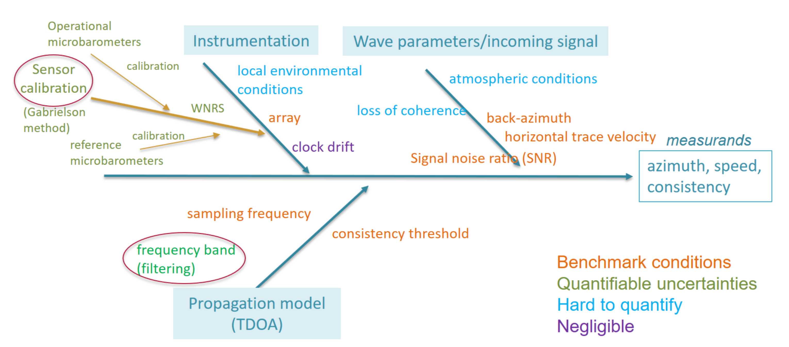
2.2. Analysis of the Measurement Process

As a first step in uncertainty propagation, a comprehensive review of uncertainty sources must be conducted by analyzing the measurement process. For complex measurement processes, such as the estimation of back azimuth and trace velocity of an incoming infrasound wave in this paper, a graphical tool such as an Ishikawa diagram (also called a fishbone diagram) is often necessary. As an example, Figure 4 displays the uncertainty sources considered in this paper that can affect the estimation of the back azimuth and trace velocity. These include uncertainty sources targeting the incoming signals (such as loss of coherence and noise), the instrumentation (such as microbarometers, calibration system, wind noise reduction system, and environmental sensitivity), and the estimation method (TDOA and Monte Carlo method).
A second step in uncertainty propagation involves quantifying the most influential uncertainty sources. Each source of uncertainty is discussed among experts to determine the availability of data or information (such as expertise, calibration results, or tabulated values) needed to quantify the associated uncertainty. For this study, the only quantifiable source of uncertainty is sensor calibration. A deeper investigation into sensor calibration reveals additional sources of uncertainty that should also be included in the Ishikawa diagram, as shown in Figure 4. The quantification and propagation of sensor calibration uncertainty is the main focus of this paper and is addressed in Section 2.3.
All of the other uncertainty sources are either too hard to quantify (at no reasonable cost) or negligible. For example, in the application, we demonstrate in Section 3.1 that the effect of filtering due to TDOA is negligible. A whole set of uncertainty sources regards those defining so-called benchmark conditions, meaning that a continuous description of the effect of the uncertainty source is not of interest, such as the array configuration or the sampling frequency. For these variables, it is more interesting to compare results in different conditions. For this reason, in this paper, we choose to study the effect of the signal/noise ratio (SNR), defective WNRS, and sensor array by treating them as scenario variables.

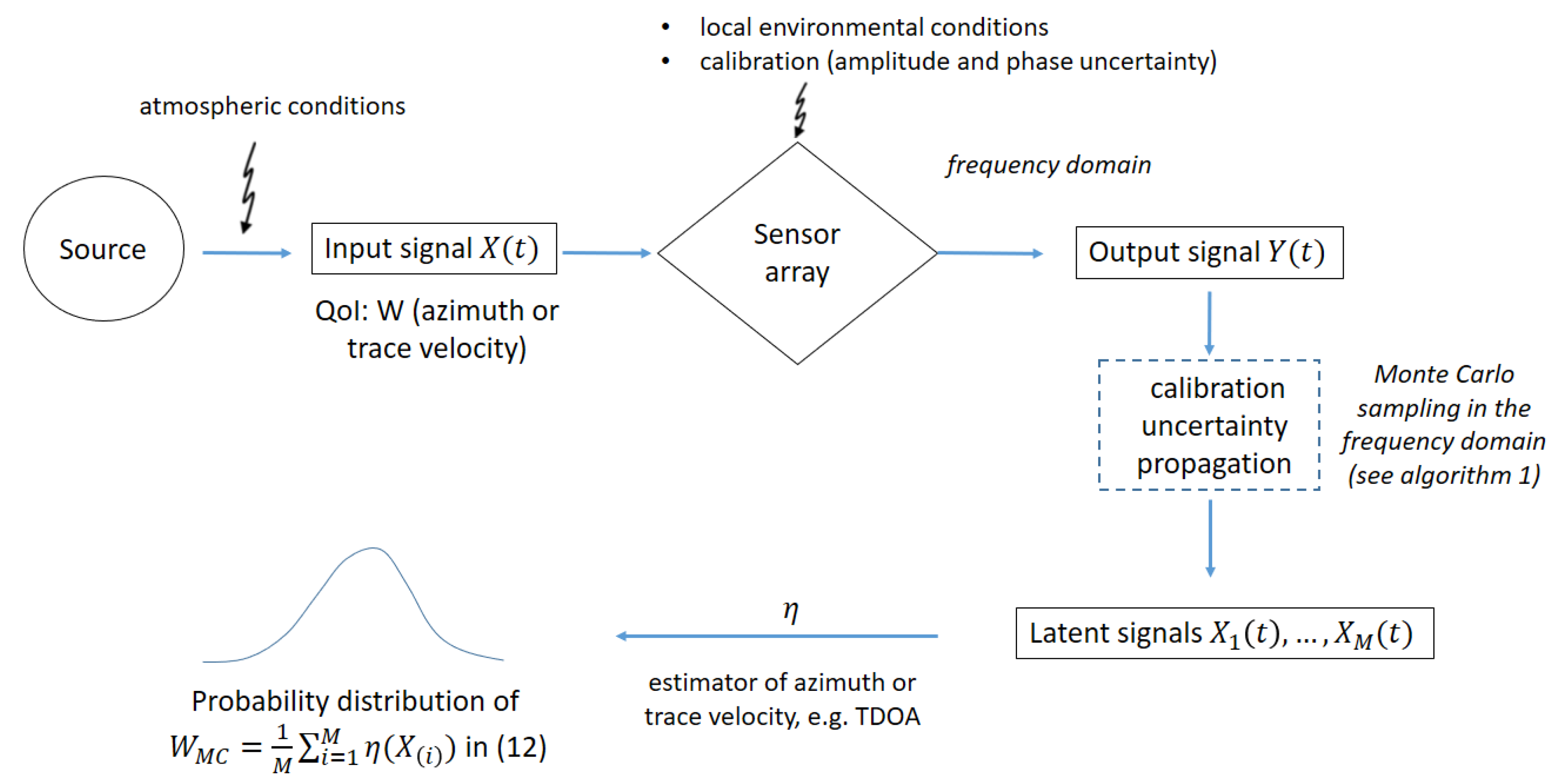
2.3. Proposed Methodology for Modeling and Propagating Sensor Calibration Uncertainty

The modeling of the microbarometer calibration uncertainty and the sensor calibration uncertainty are extensively described in Section 2.3.1, Section 2.3.2 and Section 2.3.3. Uncertainty propagation is performed with a Monte Carlo simulation method [47,48] described in Section 2.3.4, which applies to quantifiable uncertainty sources, such as sensor calibration, which is the focus of this paper.

2.3.1. Modeling Microbarometer Calibration Uncertainty

The microbarometer transfer function is obtained from the calibration of the microbarometer (see Figure 5), which must be converted from an amplitude and phase into a complex transfer function, given in V/Pa. The amplitude of the response, converted from dB V/Pa, is
a M B = 10 a M B , d B 20 ,
where a M B , d B is the amplitude given in dB V/Pa. The uncertainty of the amplitude response, also converted from dB V/Pa, is
u A M B = 10 2 a M B , d B 20 1 20 ln 10 u A M B , d B 2 ,
where u A M B , d B is the microbarometer uncertainty in dB V/Pa.
The phase of the response, ϕ M B , and its associated uncertainty, u Φ M B , are directly taken from the calibration curves and converted from degrees to radians. It is important to note that this procedure is applied to all microbarometers used in the study; therefore, H 0 or H 1 is substituted for H M B in later sections of this paper.
Although this calibration response is for an MB2005, the MB3 has comparable uncertainty since the uncertainty of the calibration is dominated by the calibration apparatus, which is the same for both types of microbarometers.

2.3.2. Determination of the Gabrielson Transfer Function

The determination of the sensor response relative to the reference microbarometer, H c a l , is obtained using the calibration procedure described by Gabrielson [31]. A reference sensor is placed next to the sensor under test, which includes a pipe-style rosette WNRS. Since the reference sensor does not include a filtering system, the response of this sensor is known via a laboratory calibration (see Figure 5). The relative response of the sensor to the reference ( H c a l ) is determined from the ratio of the auto-spectrum of the sensor under test and the cross-power spectrum of the sensor under test and the reference, as follows:
H c a l = H 1 H 0 = G 11 G 10 ,
where G 11 is the auto-spectrum of the sensor-under-test signal, G 10 is the cross-spectrum of the sensor-under-test signal and reference signal, H 0 is the response of the reference sensor, and H 1 is the response of the sensor under test (microbarometer and WNRS).
The power spectra were determined for short windows of the time series, which were stepped by 50% of the window length. Therefore, many individual measures of the frequency response were determined. The overall response was determined by taking the weighted mean of these windowed responses, and the uncertainty is the standard deviation. This procedure and experiments used to provide the calibration data used in Figure 6, Figure 7 and Figure 8 performed at CEA are described in more detail in Kristoffersen et al. [28].
Figure 6 shows the resulting response of the rosette-style pipe filtering system, including the associated uncertainties. It is worth noting that the dip in amplitude observed between 0.01 Hz and 0.08 Hz is due to partial coherence of the wind noise, as discussed by Gabrielson [31]. Although several methods have been tested to remove this dip (see, e.g., [36]), it does not affect the phase, and the expected impact on the QoI is negligible. Therefore, no additional processing of the WNRS response will be performed in this study.
Testing of WNRS systems with defects was also undertaken in this paper. An example of a defective WNRS, with 8 blocked (out of 32) inlets is shown in Figure 7. This response can be used to replace the response of one of the sensors, in order to see the effects of a defective sensor on the measurement uncertainty. An example of a defective sensor will also be discussed in the results.

2.3.3. Modeling the Uncertainty Associated with the Sensor

H s e n is the complex frequency response of the sensor, defined as
H s e n = H c a l H 0
where H 0 and H c a l are the reference microbarometer and the Gabrielson transfer functions, described in Section 2.3.1 and Section 2.3.2, respectively. Hence, by multiplying H c a l by the reference microbarometer response, H 0 , one arrives at the sensor response, given in V/Pa.
Equivalently, the sensor response can be expressed as
H s e n = A s e n e j Φ s e n ,
where A s e n and Φ s e n are the sensor’s amplitude and phase distributions obtained from the sensor calibration frequency response, respectively.
The best estimates of the amplitude and phase of the sensor’s complex response are given by a s e n = a c a l a 0 and ϕ s e n = ϕ c a l + ϕ 0 , respectively, where a c a l , ϕ c a l are obtained from the Gabrielson calibration responses and a 0 and ϕ 0 are obtained from the laboratory calibration of the reference microbarometer.
For each frequency, these responses are treated as Gaussian distributions:
A s e n = a s e n + ε A s e n ,
Φ s e n = ϕ s e n + ε Φ s e n ,
where ε A s e n N 0 , u A s e n , ε Φ s e n N 0 , u Φ s e n , u A s e n , and u Φ s e n are defined in (17) and (18), respectively.
The final model for the uncertainty assessment associated with the sensor amplitude and phase are, respectively, expressed as
u A s e n 2 = a s e n 2 u A c a l a c a l 2 + u A 0 a 0 2 ,
u Φ s e n 2 = u Φ c a l 2 + u Φ 0 2 ,
where u A c a l , u Φ c a l are obtained from the Gabrielson calibration responses and u A 0 and u Φ 0 are obtained from the calibration certificate of the reference sensor. The sensor response is shown in Figure 8.

2.3.4. Monte Carlo Method Using Latent Input Signals for Uncertainty Propagation

The Monte Carlo method [47,48] is usually used for the estimation of integrals, as is the case in this paper with the quantity of interest W defined as an integral in (2). For deconvolution problems, such as the estimation of X in (1), the Monte Carlo method is applied in the frequency domain [41]. In this section, we show how to apply the Monte Carlo method in the frequency domain to estimate the QoI W, assuming that the transfer function of the sensor H s e n is known.
In the frequency domain, the input signal X ^ ( f ) can be obtained from (1) as
X ^ ( f ) = Y ^ ( f ) H s e n ,
where Y ^ ( f ) is the observed output signal in the frequency domain obtained by taking the Fourier transform of Y ( t ) .
Back in the time domain, the estimated input signal X ( t ) is obtained from (19) by taking the inverse Fourier transform
X ( t ) = F 1 X ^ ( f ) .
Algorithm 1 shows how to generate M Monte Carlo samples X ( 1 ) , , X ( M ) (called latent signals in the paper, also see Figure 1) from (20) independently with the same distribution, denoted π in (2), when the calibration uncertainty is known and modeled, as in Section 2.3.3.
The Monte Carlo estimator W M C of W is given by
W M C = i = 1 , , M η ( X ( i ) ) M ,
where η is defined in (2) and in Section 2.1.
Algorithm 1: Algorithm for sampling latent signals from (20).
Data: transfer function of the sensor H s e n defined in (14), observed output signal
Y ( t ) , number of Monte Carlo simulations M
Result: M latent signal X ( 1 ) , , X ( M ) sampled from (20)
while  i M  do
generate a i N ( a s e n , u A s e n ) according to (15); /* sample latent signal
amplitude /*
generate ϕ i N ( ϕ s e n , u Φ s e n ) according to (16); /* sample latent signal
phase */
compute h i = a i e j ϕ i ;
compute X ^ i ( f ) = Y ^ ( f ) h i ;
X ( i ) F 1 X ^ i ( f )
end
The estimator (21) is a random variable. Denoting x ( i ) the actual realization of X ( i ) , the point estimation of the QoI W, denoted W ^ M C , is obtained by replacing X ( i ) with x ( i ) in (21). The performance of the estimator W M C is assessed on the generated Monte Carlo sample { x ( 1 ) , , x ( M ) } with the empirical bias, standard deviation, MAE, and RMSE, defined as follows.
The bias, also referred to as error throughout the paper, is estimated as
b i a s ( W M C ) W ^ M C W .
The distribution of bias (error) is the distribution of the vector of observed biases ( b 1 , , b M ) estimated on the Monte Carlo sample { x ( 1 ) , , x ( M ) } with b i defined as
b i = η ( x ( i ) ) W .
The standard deviation is estimated as
σ ( W M C ) 1 M i = 1 M η ( x ( i ) ) W ^ M C 2 .
The MAE, mean absolute error, is estimated as
M A E ( W M C ) 1 M i = 1 M | η x ( i ) W | .
The RMSE, root mean squared error, is estimated as
R M S E ( W M C ) 1 M i = 1 M η ( x ( i ) ) W 2
It can be noticed that these indicators depend on M. A larger number of samples would increase the confidence in the Monte Carlo estimate by decreasing its variability but not its bias. This is known as the variance–bias compromise in statistics.

3. Results

In this section, we illustrate the methodology for calibration uncertainty propagation with the Monte Carlo method to estimate the back azimuth and trace velocity of an incoming infrasound signal at a station, using synthetic output signals from existing array designs (OHP, IS26, …). The array designs that are used in this study are shown in Figure 9. Each array consists of between 4 and 9 sensors, with apertures between about 1 and 3 km.
The calibration uncertainty information is experimentally determined and displayed in Figure 5 for the MB2005 response, in Figure 6 for the WNRS response, and in Figure 8 for the sensor response. In Section 3.1, calibration uncertainty is propagated for infinite SNR and operating WNRS. In Section 3.2, a sensitivity study is performed to show the effect of the SNR, the WNRS, and the station array aperture on the estimates of the back azimuth and trace velocity. A further study on the effects of different amounts of sensor phase uncertainties was performed to determine the acceptable levels of sensor phase uncertainties as functions of the frequencies for infrasound stations. The results are given as functions of the frequencies. The performance of the Monte Carlo estimates is analyzed in terms of bias, standard deviation, MAE, and RMSE, as defined in (22), (24), (25), and (26), respectively. The distribution of bias (error) displayed in Figure 10, Figure 11, Figure 12, Figure 13, Figure 14 and Figure 15 and in Appendix B, Appendix C and Appendix D is obtained according to (23).

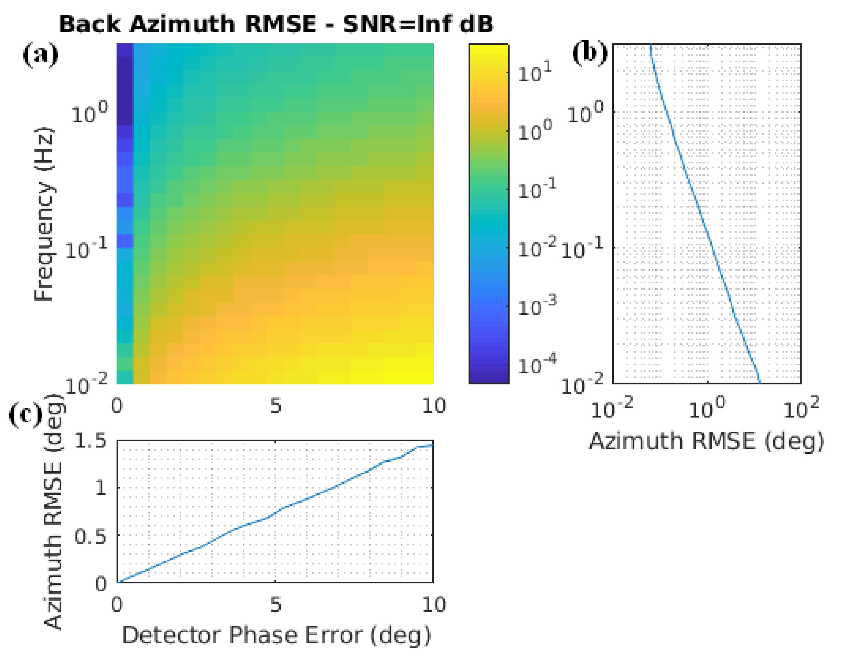
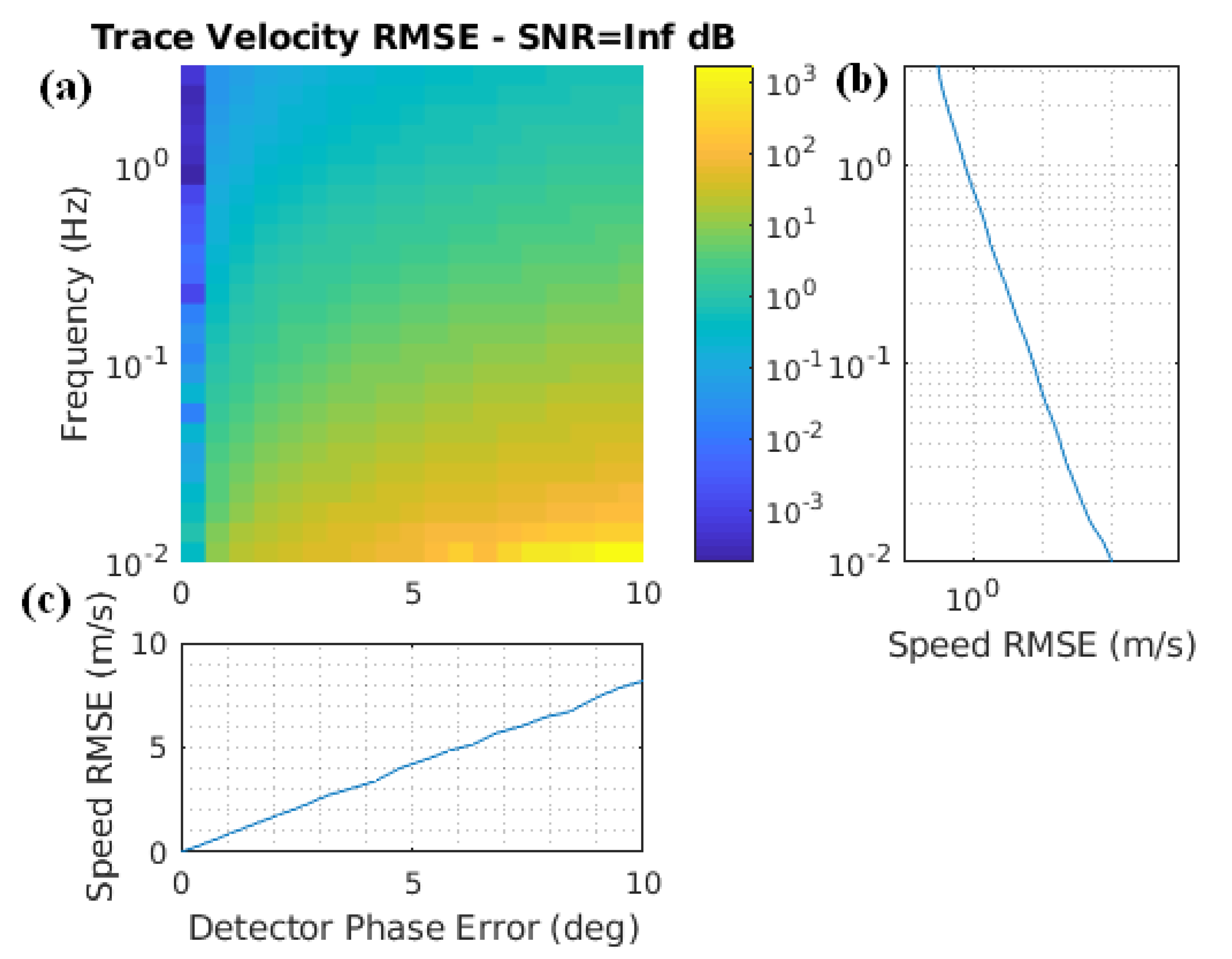
3.1. Uncertainty Propagation Results for Infinite SNR and Operating WNRS

The methodology of uncertainty propagation is applied to a synthetic signal generated as a potential signal output of the sensor array of the Observatoire de Haute Provence (OHP, see Figure 9 for the array design), according to Appendix A with an infinite SNR. For this signal, back azimuth and trace velocity are known so that the QoI W is known. In this paper, due to the computational time, the number of Monte Carlo simulations is M = 10 4 .
A slight (non-significant) bias was observed for both back azimuth and trace velocity, see Figure 10 and Figure 11. For the back azimuth, the errors are smaller than the uncertainty; however, for the high-frequency trace velocity results, there are observable biases. Working with a known input signal will allow us in this particular case to investigate the origin of this bias.
We begin by considering a signal generated using ideal microbarometers, with an infinite signal-to-noise ratio (SNR), and no other uncertainty sources except for those present in the signal generation and TDOA analysis. The errors in back azimuth and trace velocity for such a signal are shown in Figure 12 and Figure 13. In this case, the dispersion shown by the boxplots is due to the variability observed from a single run of the TDOA algorithm, such as that shown in Figure 2 for each frequency band. As can be observed, for both the back azimuth and trace velocity, there are statistically significant biases at almost every frequency. It should also be noted that these biases follow the same trend as shown in Figure 10 and Figure 11. This demonstrates that there is a bias introduced by the signal generation and by the TDOA-filtering procedures. However, these values are typically small compared to the observed variability, even for the infinite SNR scenario. Therefore, in practice, these biases can be considered negligible. For the purposes of this study, given that the biases are known a priori, we decided to remove them from the Monte Carlo results.
Further study is needed to identify the exact cause of these biases in the signal analysis routines, but this was determined to be outside the scope of this paper. Additionally, given the small value of the biases relative to the variances of the quantities of interest, particularly once the noise is introduced, the biases are not likely to be observable under true measurement conditions.

3.2. Sensitivity Study

In this section, a sensitivity study is performed to show the effect of the SNR, the WNRS, and the station array aperture, called benchmark conditions in Section 2.2, on the estimates of the back azimuth and trace velocity. For all configurations, the bias due to filtering or signal generation is removed according to Section 3.1 so that no effect due to filtering can be observed in the results.

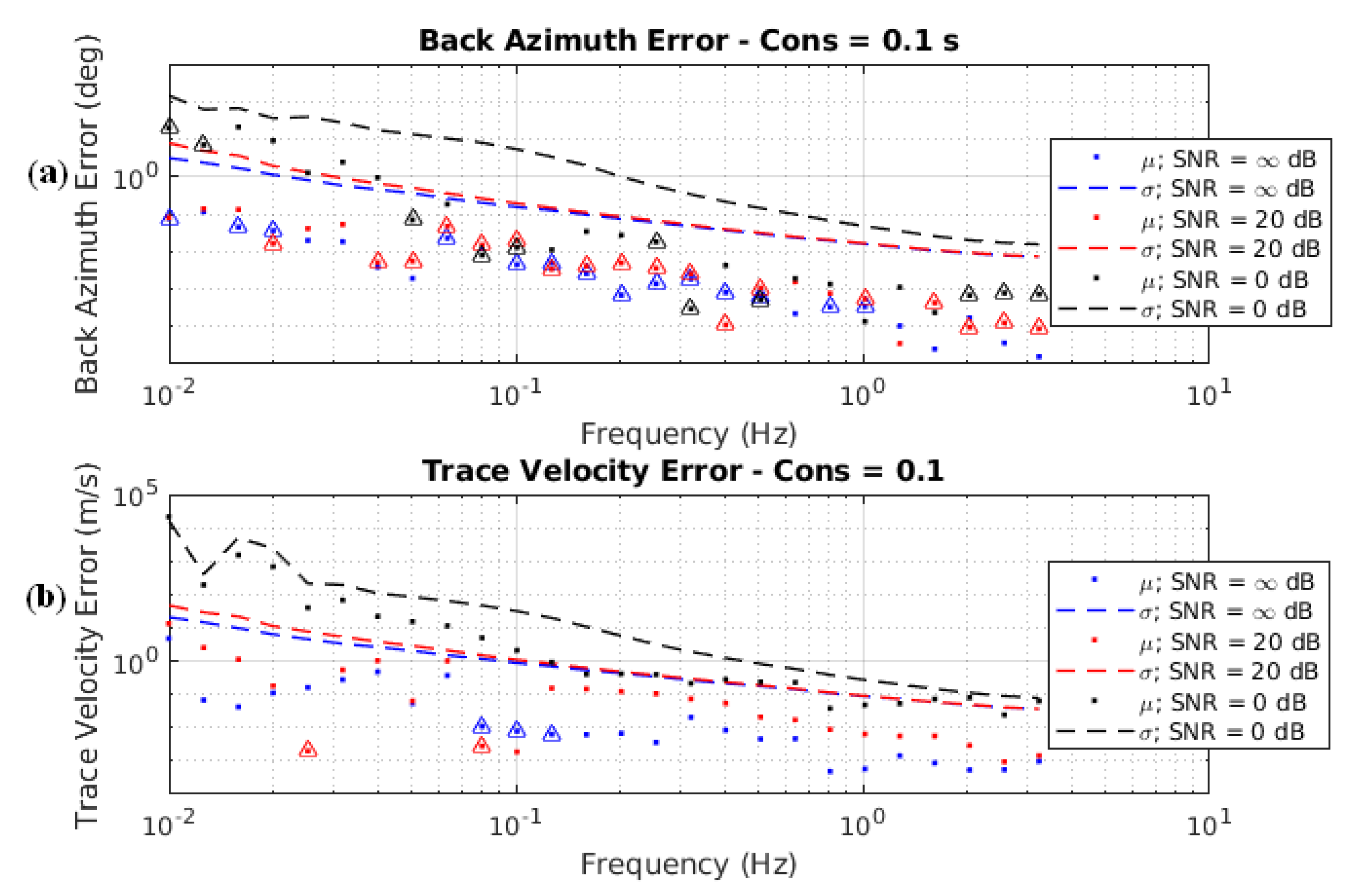
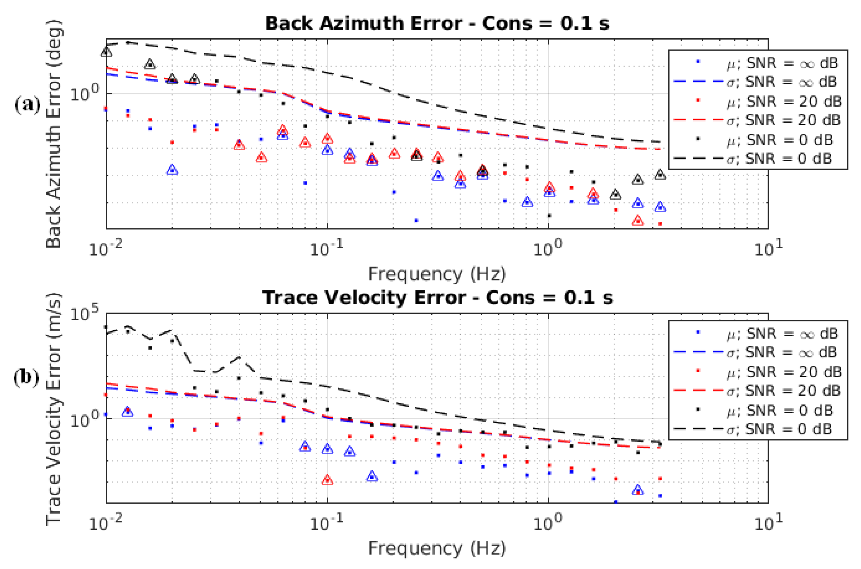
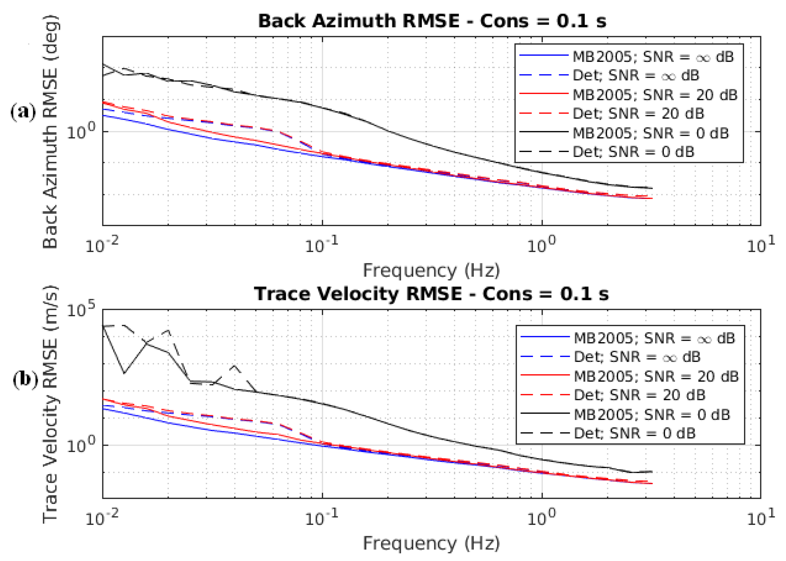
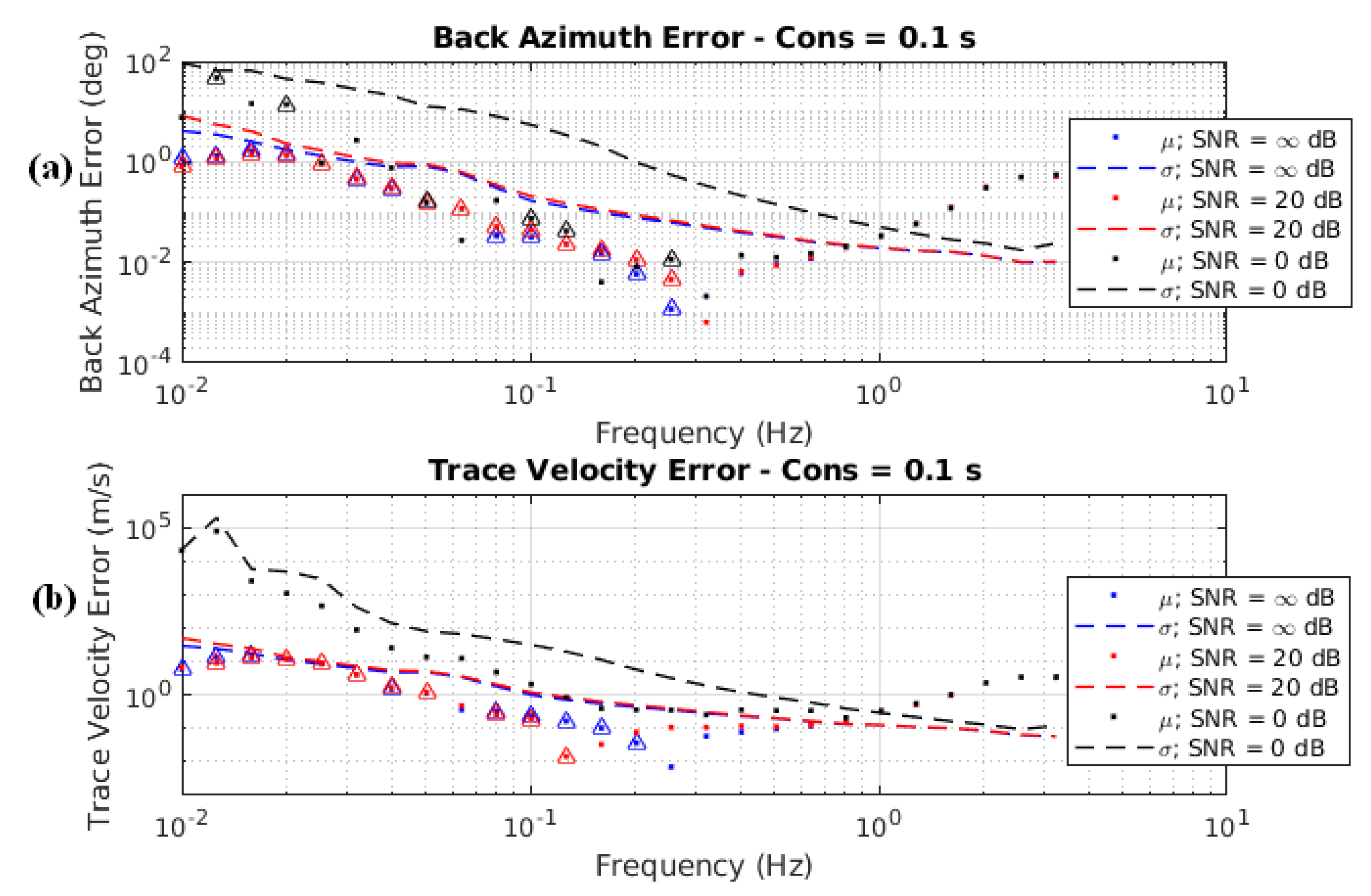
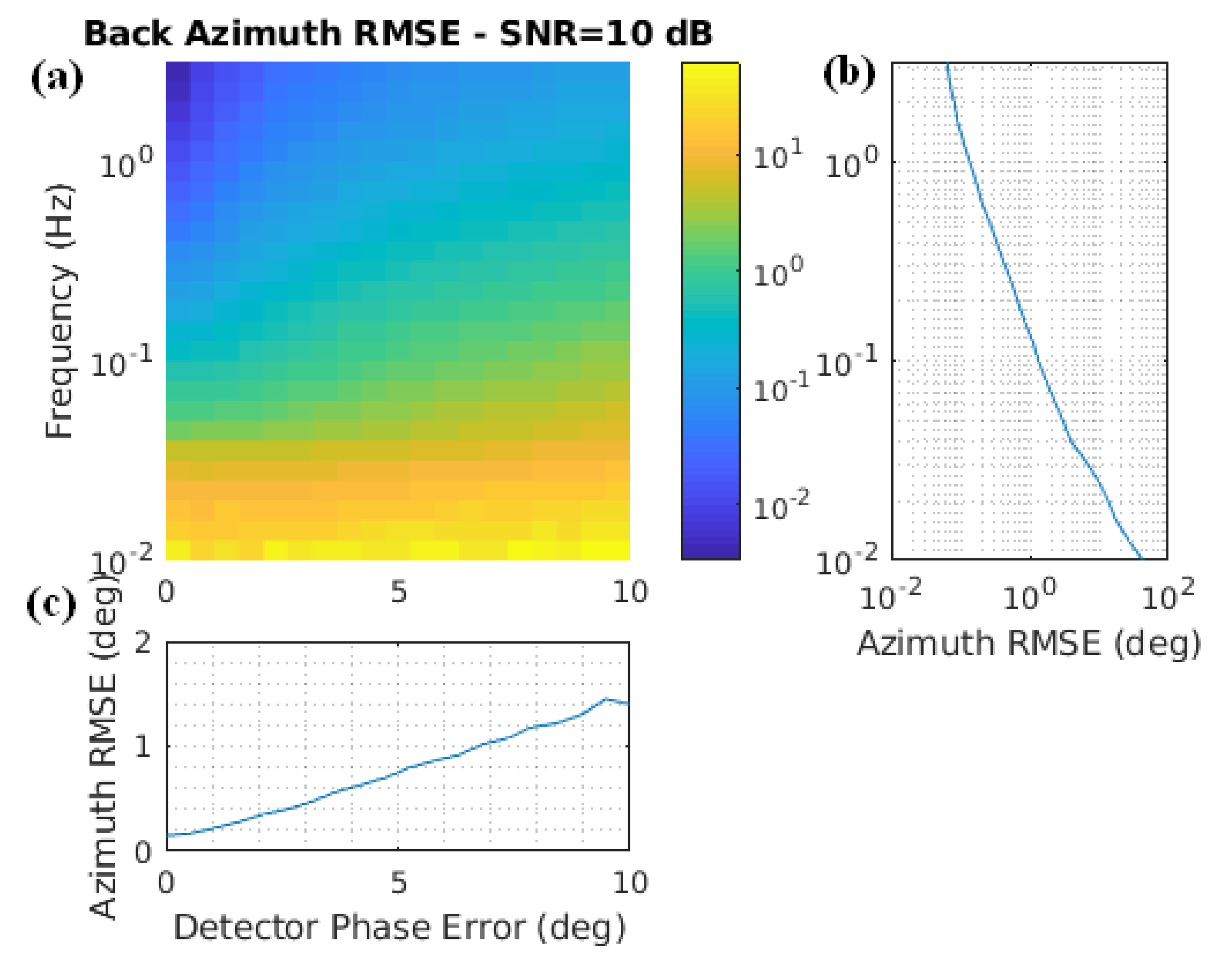
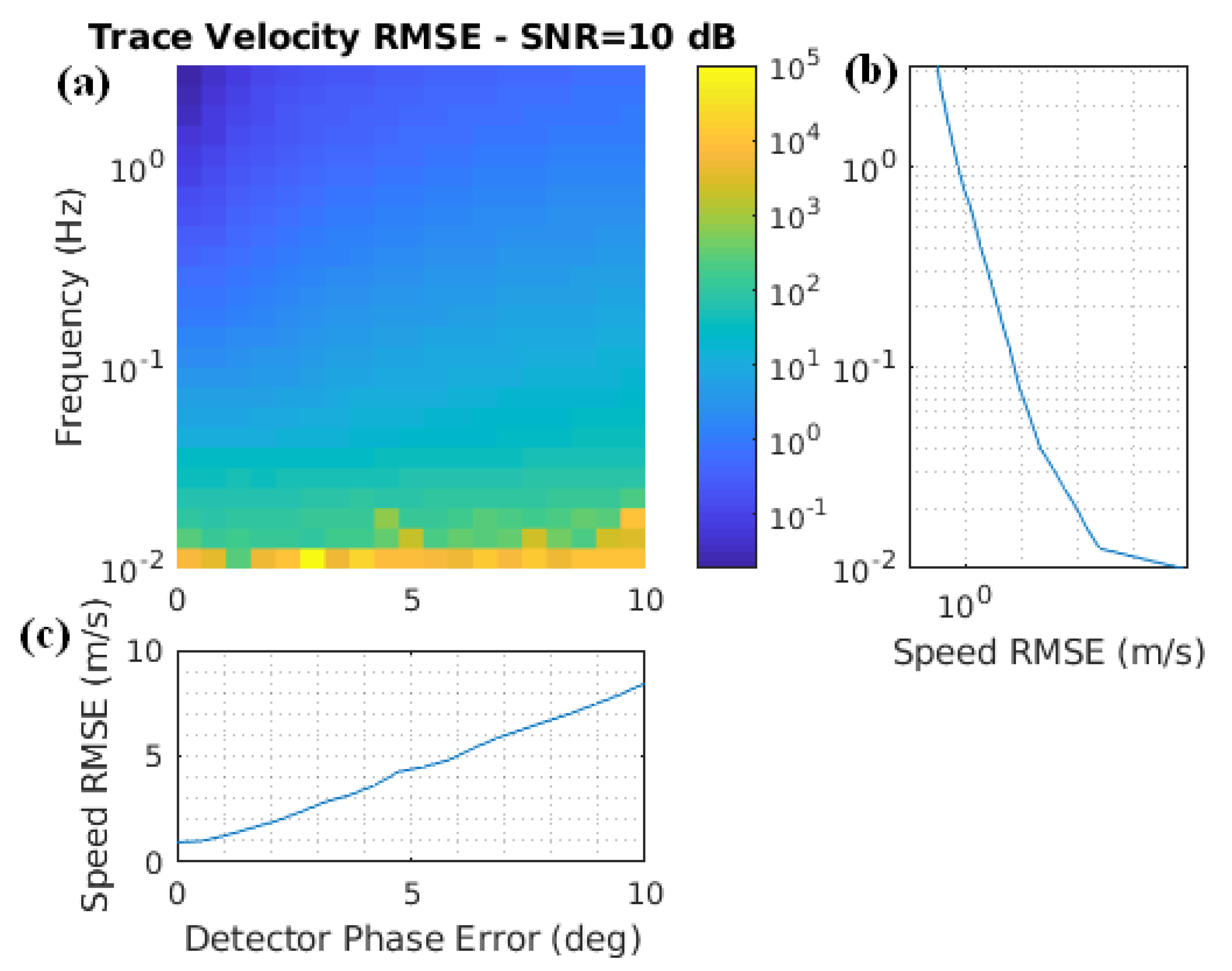
3.2.1. Results for Different SNR

The objective of this section is to analyze the effects of the SNR (infinite, 20 dB, 0 dB) on the Monte Carlo estimation of the back azimuth and trace velocity when the sensor uncertainty is taken into account.
To begin, we will focus on the microbarometer (see Figure 5 for a typical MB2005/MB3 response). The resulting uncertainties caused by the MB2005/MB3 microbarometers are shown in Figure 14, where the dots represent the MAE and the dashed lines represent the standard deviation. As expected, the uncertainty decreases with increasing frequency and with increasing SNR. As the frequency increases, the uncertainty begins to converge and approaches the no-noise limit. The higher the SNR, the lower the frequency at which the uncertainty converges with the no-noise limit. The errors themselves do not appear to be preferentially positive or negative, suggesting that the errors remain randomly distributed around 0. Additionally, it is clear that the errors are always within the uncertainty bounds, indicating negligible bias at all frequencies.
Next, the resulting errors caused by the sensor, which are the microbarometer and WNRS, are shown in Figure 15. Once again, the uncertainty decreases with both the increasing frequency and SNR. The errors have a negligible deviation from 0, considering the values of the uncertainty. The sensor results are very similar to those of the microbarometer. A comparison between the RMSE of the microbarometer and sensor, shown in Figure 16, shows that the sensor errors at low frequencies (below 0.1 Hz) are typically larger than those of the microbarometer. This is caused by increased uncertainty in the sensor calibration at a low frequency due to a partial coherence of the wind-generated noise [31,36]. At higher frequencies, this increased error is much smaller. The difference in error also decreases with decreasing SNR. Therefore, at a lower SNR, there is no discernible difference between the microbarometer alone and the whole sensor.
Histograms of the errors (after bias removal according to Section 3.1) at each of the 26 frequencies for back azimuth and trace velocity, and SNR equals infinity, 0 dB and 20 dB are displayed in Appendix B, Appendix C and Appendix D, respectively.

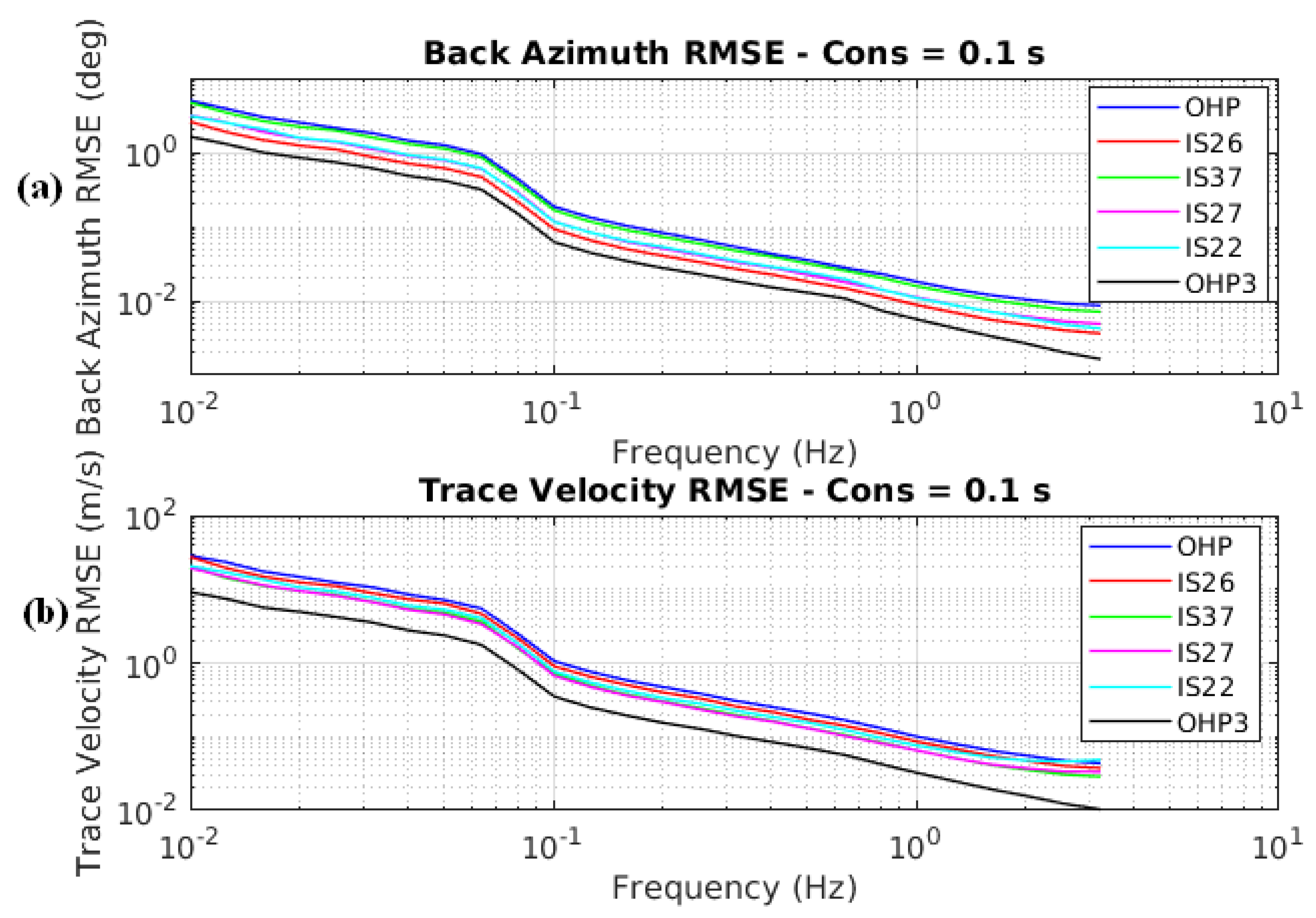
3.2.2. Results for Different Sensor Arrays

The design of the sensor array, including its size and shape, has been shown to have an impact on the precision and accuracy of infrasound detections [8,20]. Previous studies have investigated uncertainties associated with the sensor array [20], but they have used the sampling frequency as a measure of time measurement uncertainty. In this study, sensor uncertainty is determined through calibration, including amplitude and phase. Array apertures can range from 10 m for a small high-frequency array to several kilometers (1–3 km for IMS stations). Typically, a larger aperture array will be more precise but may experience aliasing issues at higher frequencies. However, a very dense large aperture array could avoid these issues, but practical limitations such as site availability and cost must also be considered in designing the array. It is, therefore, of interest to study the effects that different arrays may have on the TDOA output parameters. Therefore, several different array designs of existing stations were considered, the Observatoire de haute-provence (OHP), IS22 in New Caledonia, IS26 in Germany, IS27 in Antarctica, IS37 in Norway, and a synthetic array that was the same design as OHP but three times larger, hereinafter referred to as OHP3. These arrays were chosen to provide several different array sizes and shapes, including arrays with different numbers of sensors. However, all of these synthetic data suppose a temperature of 23 ° C and pressure of 1000 hPa. In this manner, only the effects of the sensor array size and shape were considered; for real station data, the different environmental conditions would affect the results.
The results for these six different arrays are shown in Figure 17. Given that IS22 (cyan), a triangle with a four-central element, is largely the same as OHP (blue) but larger, and OHP3 (black), a larger array will return smaller root-mean-squared errors in both back azimuth and trace velocity. There appears to be little correlation between the number of sensors and the errors. However, it should be noted that these analyses do not include decoherence of the infrasound beam form, which would greatly affect the results such that the arrays with small subnets would be better at measuring signals with high decoherence. Decoherence (or loss of coherence) is the result of the finite size of the beam form caused by small variances in the wavenumber. Therefore, as measurements are made further apart, there will be a decrease in coherence until there is no coherence between the measurements at sufficiently large distances. For the purpose of this study, it has been assumed that this decoherence is negligible over the length scales of the arrays that were used.
It is worth noting that stations with approximately the same-sized apertures (IS22, IS26, IS27, IS37) have inverted orders in terms of back azimuth and trace velocity RMSE. However, this is caused by the complementarity of the back azimuth and trace velocity uncertainties as a function of the back azimuth angle. That is to say, at angles where the back azimuth uncertainty is smaller, the trace velocity uncertainty is larger, and vice versa. Therefore, this apparent inversion of the order of the RMSE is due to the choice of back azimuth for the input signal. If all back azimuths were considered, then the order of the mean RMSE would be the same for both back azimuth and trace velocity. In such a case, the RMSE would be, in descending order, OHP, IS22, IS37, IS26, IS27, and OHP3.

3.2.3. Results for a Defective WNRS

Regarding the infrasound station, it is worth considering the effects due to defective WNRS, i.e., a WNRS, which has blockages or leaks. Since there are an enormous number of different combinations of defects and WNRS designs, a single defective system was chosen. Using the same nominal system which has been used throughout the paper (see Figure 6), one of the four sensors was considered to be defective with eight (one-quarter) of the inlets blocked, as shown in Figure 7. The same Monte-Carlo calculations as presented in Section 3.2.1 were performed using this array with one defective WNRS.
For this defective system, there is a noticeable increase in the observed errors for both the back azimuth and trace velocity, as shown in Figure 18. This is quite evident in the no-noise case (blue lines), as, starting around 1 Hz, the errors begin increasing. However, the uncertainties are still trending downward with very small values above 1 Hz. This results in non-negligible biases in both the back azimuth and the trace velocity. As the SNR is decreased, the uncertainties and errors at all frequencies increase, with the exception of the errors near the WNRS resonance peak (2–3 Hz), which approach the same values for all three noise cases (it should be noted that, above 1 Hz, the blue and red dots are hidden behind the green dots). This suggests that a defective WNRS would act as an error floor for a system, and as the noise or other sources of uncertainty increase, the effects of the defect would become less evident. Of course, as the noise and other sources of uncertainty increase, the measurement uncertainty would also increase.

3.3. Sensor Phase Uncertainty

For the IMS stations, the CTBTO has defined an acceptable limit of ± 5 % for the sensor response [9,36]. Therefore, it is important to investigate the effects of sensor uncertainty on the output parameters and to determine acceptable sensor uncertainty thresholds for these stations. Since phase plays a crucial role in the calculation of back azimuth and trace velocity using TDOA, the focus is on phase uncertainty rather than amplitude uncertainty. Any phase error in a signal measured by a sensor will result in a corresponding error in the time of arrival of the signal, which is inversely proportional to the frequency. Additionally, the sensitivity to phase errors will depend on the array size, with smaller arrays being more sensitive.
To study the effects of different levels of phase errors on the back azimuth and trace velocity calculations, the phase errors were set to a single value over the entire frequency range of interest (0.01–4 Hz), and varied between 0 and 10 to see the effects of different phase errors on the final results. The differences between the expected back azimuth and trace velocity were calculated. Figure 19 and Figure 20 show the RMSE for the back azimuth and trace velocity, respectively. As was previously observed in Section 3.2.1, there is a strong frequency dependence on the errors, with the errors decreasing with increasing frequency. As would be expected, there is also an increase in errors with an increase in sensor uncertainty. At high frequencies (>1 Hz), the observed errors are low, even up to a 10 uncertainty for the sensor. However, at low frequencies (<0.1 Hz), the errors can be quite large (several degrees and 10 m/s) at even small sensor uncertainties.
At a lower SNR of 10 dB, the results are similar, with an increase in the overall errors, as shown in Figure 21 and Figure 22. It should be noted that there are far fewer values that are below the consistency threshold for frequencies lower than 0.025 Hz. This is why there is additional variability at these very low frequencies. Overall, there is a similar trend as with the no-noise case. However, more low-frequency events are missed at an SNR of 10 dB.
Overall, it can be concluded that at high frequencies, sensor errors of less than 5° should not greatly impact results, with other factors such as decoherence and SNR being more important. At low frequencies, sensor errors can have significant impacts on the results, even as little as 2° can result in errors larger than 5° and 20 m/s in back azimuth and trace velocity, respectively. This analysis was performed using the OHP array, with an aperture of approximately 1.2 km. For an array of a significantly different size, a similar analysis with those dimensions would need to be performed. It is, therefore, of use to perform this type of analysis when designing an infrasound array to determine if the sensor is sufficiently precise for the frequency band of interest.

4. Conclusions

In an attempt to determine the effects of the sensor uncertainty on the parametric outputs of the TDOA algorithms for infrasound stations, a propagation of the sensor uncertainty was accomplished. First, the in situ calibration of the sensor was performed using a reference sensor with a known calibration response. Then, after generating a synthetic signal, where we had a synthetic sensor output signal, the signal was deconvolved with the sensor response, including the uncertainty, to provide a latent signal with the measured sensor uncertainties. This latent signal was then used as an input to the TDOA algorithm, providing distributions of the QoI, the back azimuth, and the trace velocity.
Overall, this approach was fruitful, as the distributions of the back azimuth and trace velocity, as functions of frequency, were successfully determined at several different SNR levels for the microbarometers alone, and the sensor (microbarometer and WNRS). The resulting errors in back azimuth and trace velocity were unbiased, with the errors increasing dramatically with decreasing frequency. For example, for the sensor case, at the highest frequency, the back azimuth and trace velocity errors were 0.01° and 0.1 m/s, respectively. However, at the lowest frequency, these errors were 5° and 30 m/s, respectively. This was due to the relative decrease in the phase resolution of the infrasound wave at lower frequencies.
Additionally, the uncertainty was inversely related to the SNR. However, there was also a frequency dependence. In fact, there was no noticeable difference between the uncertainties for the infinite and 20 dB SNR cases above 0.2 Hz, with the 20 dB case having larger uncertainties at lower frequencies. Therefore, it would be possible to measure lower SNR signals at higher frequencies, or with a larger aperture station, assuming that the effects of decoherence are minimal. This Monte Carlo approach could be applied to any station configuration and SNR, and as such, could be used in the identification of ideal station designs in the future.
It was shown that the CTBTO sensor uncertainty threshold of 5% is sufficient at high frequencies, above about 0.1 Hz. However, at low frequencies, sensor phase errors of even 2° can lead to large errors in the back azimuth and trace velocity measurements. Therefore, one must be aware of how the uncertainties vary with frequency when considering the sensor uncertainty.
It is difficult to conclude which parameters have the largest impact on the results as this depends on the frequency. In general, at low frequencies (below ∼ 0.1 Hz), the phase errors in the sensor calibration result in substantial uncertainties in the QoI. At higher frequencies, the sensor phase errors result in almost no noticeable variability in the QoI, with the SNR being a much more important parameter. A full sensitivity analysis would be useful to provide a more complete estimation of the relative importance of the different parameters. An increase in the size of the array is equivalent to a decrease in the frequency.
Future work using this analysis tool would involve additional uncertainty sources, such as the loss of coherence, to consider more input back azimuth angles, or use real infrasound data in the uncertainty analysis. In addition, as previously mentioned, a sensitivity analysis would provide valuable information concerning the relative importance of the different input parameters.

Author Contributions

Conceptualization, S.D. and S.K.K.; methodology, S.D. and S.K.K.; software, S.K.K.; validation, S.D. and S.K.K.; formal analysis, S.D. and S.K.K.; investigation, S.K.K. and A.L.P.; resources, A.L.P. and F.L.; data curation, S.K.K.; writing—original draft preparation, S.D. and S.K.K.; writing—review and editing, all; visualization, S.D. and S.K.K.; supervision, F.L.; project administration, F.L.; funding acquisition, F.L. and N.F. All authors have read and agreed to the published version of the manuscript.

Funding

This project 19ENV03 Infra-AUV received funding from the EMPIR program co-financed by the participating states and the European Union’s Horizon 2020 research and innovation program.

Data Availability Statement

The calibration data presented in this study are openly available at https://doi.org/10.5281/zenodo.7785697.

Conflicts of Interest

The authors declare no conflict of interest. The funders had no role in the design of the study; in the collection, analyses, or interpretation of data; in the writing of the manuscript; or in the decision to publish the results.

Abbreviations

The following abbreviations are used in this manuscript:
F Fourier transform
RMSE root mean squared error
TDOA time difference of arrival
PMCCprogressive multi-channel correlation
QoIquantity of interest
WNRSwind noise reduction system
SNRsignal-to-noise ratio
SOIsignal of interest
CTBTOComprehensive Test Ban Treaty Organization
CEACommissariat à l’Energie Atomique et aux Energies Alternatives
OHPObservatoire de Haute Provence
IMSInternational Monitoring System
MBmicrobarometer
Htransfer function of the MB or the sensor
hmean response of the MB or the sensor

Appendix A. Signal Simulation from Sensors in an Array

To demonstrate the methodology developed in the paper for uncertainty propagation of infrasound measurements, we chose to work on a simulated signal with known wave parameters (back azimuth and trace velocity). This allowed for the comparison of results to known values and the analysis in terms of bias.
To accomplish this, we focused on synthetic broadband data. A broadband signal was chosen to enable the study of all frequency bands at once, reducing calculation time by a factor of 26.
The broadband signal is created by starting with randomly generated Gaussian noise with a mean of 0 and a standard deviation of 1. For this study, a 1-h signal sampled at 20 Hz is generated. Then, a known back azimuth and trace velocity are chosen, and the signal is shifted in time for each sensor, given the known orientations of the sensors. This step is essentially the inverse of (5), such that the time delay at the sensors is given by
τ = XY S .
This provides a signal at each sensor shifted in time relative to the other signals by an amount consistent with the known slowness and sensor array orientation. Gaussian noise is then added to the signal individually at each sensor based on the input SNR. In this manner, the noise is completely incoherent between the different sensors. Given the typical coherence length of wind is small compared to the distances between sensors for the IMS frequency band, this accurately represents the behavior of the wind noise [33]. Although the noise typically measured by infrasound sensors is not white, this color of noise was chosen to represent the correct SNR at each frequency. Since the input signals have the same amplitude at all frequencies, a ’real’ noise would result in different SNRs for each frequency band.
At this stage, the effects of the microbarometer and WNRS can be included by convolving the signal at each sensor with the nominal (that is to say, mean) response of the sensor. To do this, the signal is converted to the frequency domain by taking the Fourier transform, such that
s ^ ( f ) = F ( s ( t ) )
where s ( t ) is the synthetic signal (in Pa).
We introduce the notation h s e n , which represents the best estimate of the sensor response obtained from the calibration information using the Gabrielson method. To convert the amplitude from dB to a complex space, we use the following equation:
h s e n ( f ) = 10 a d B , s e n 20 e j ϕ s e n ,
where a d B , s e n is the amplitude given in dB and ϕ s e n is the phase in radians.
The signal is then convolved with the sensor response, resulting in the simulated sensor output:
y ^ ( f ) = s ^ ( f ) h s e n .
This sensor output is the signal measured at each microbarometer in the array.

Appendix B. Results with SNR = Inf

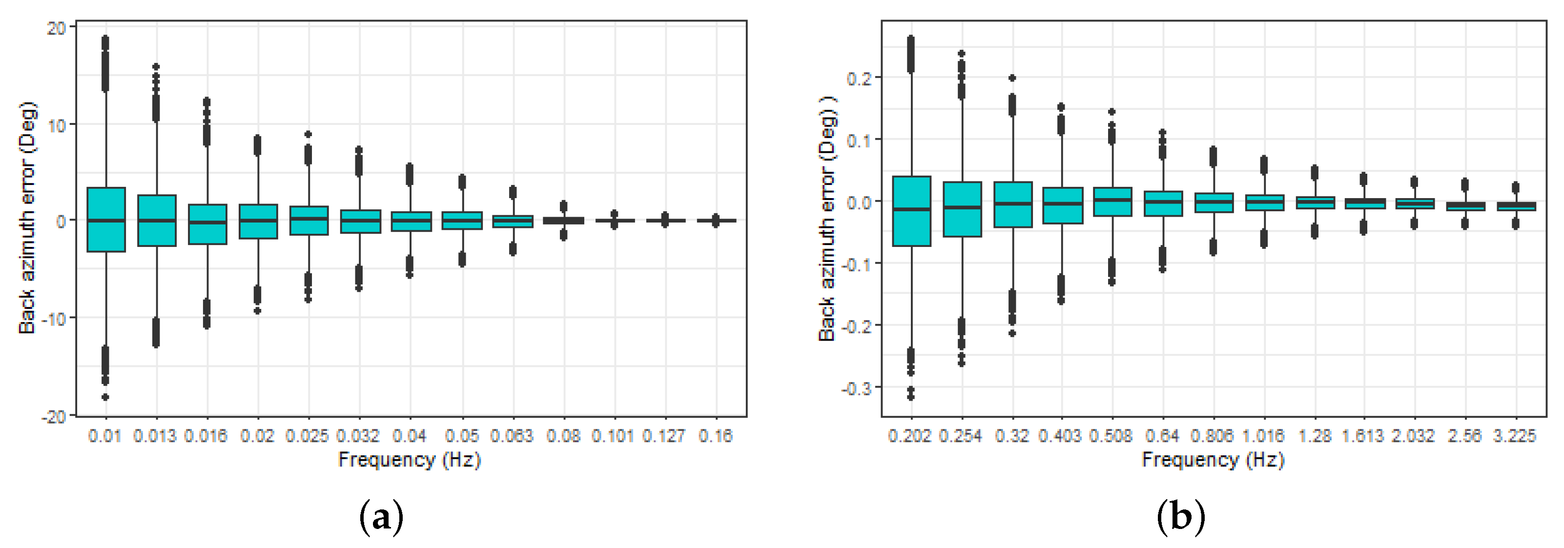
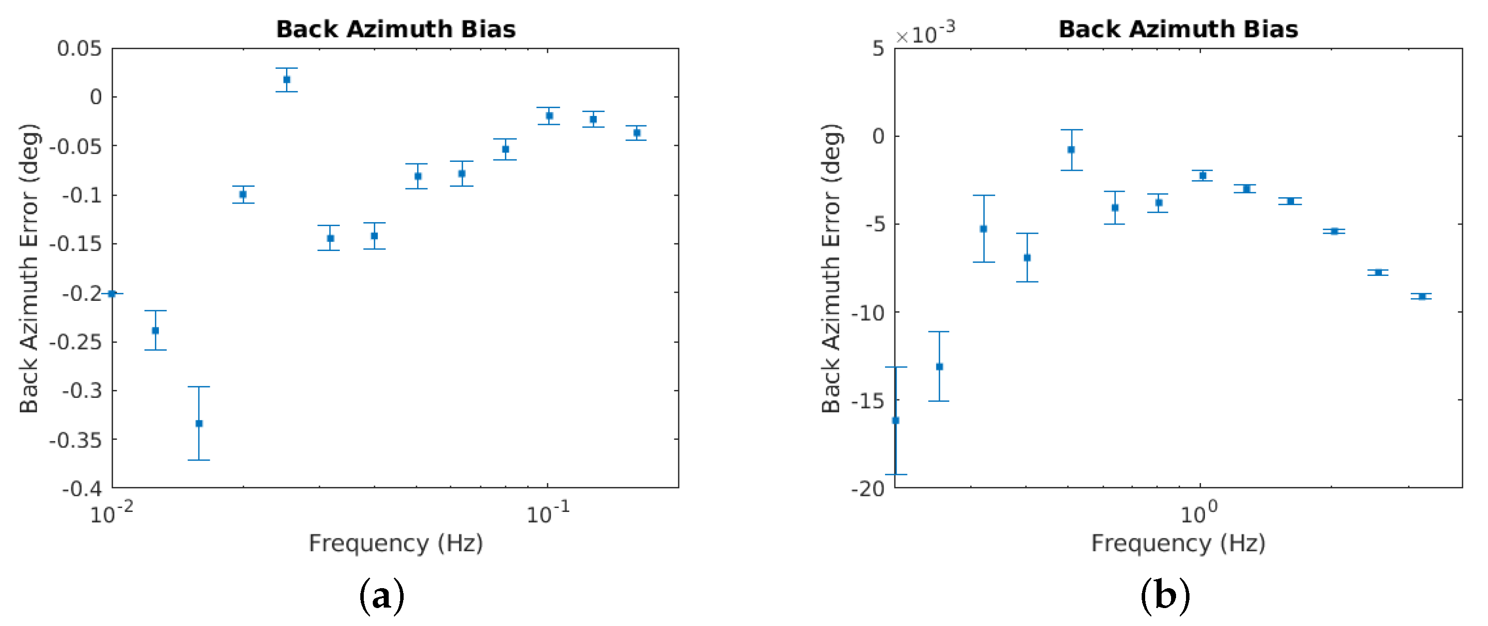
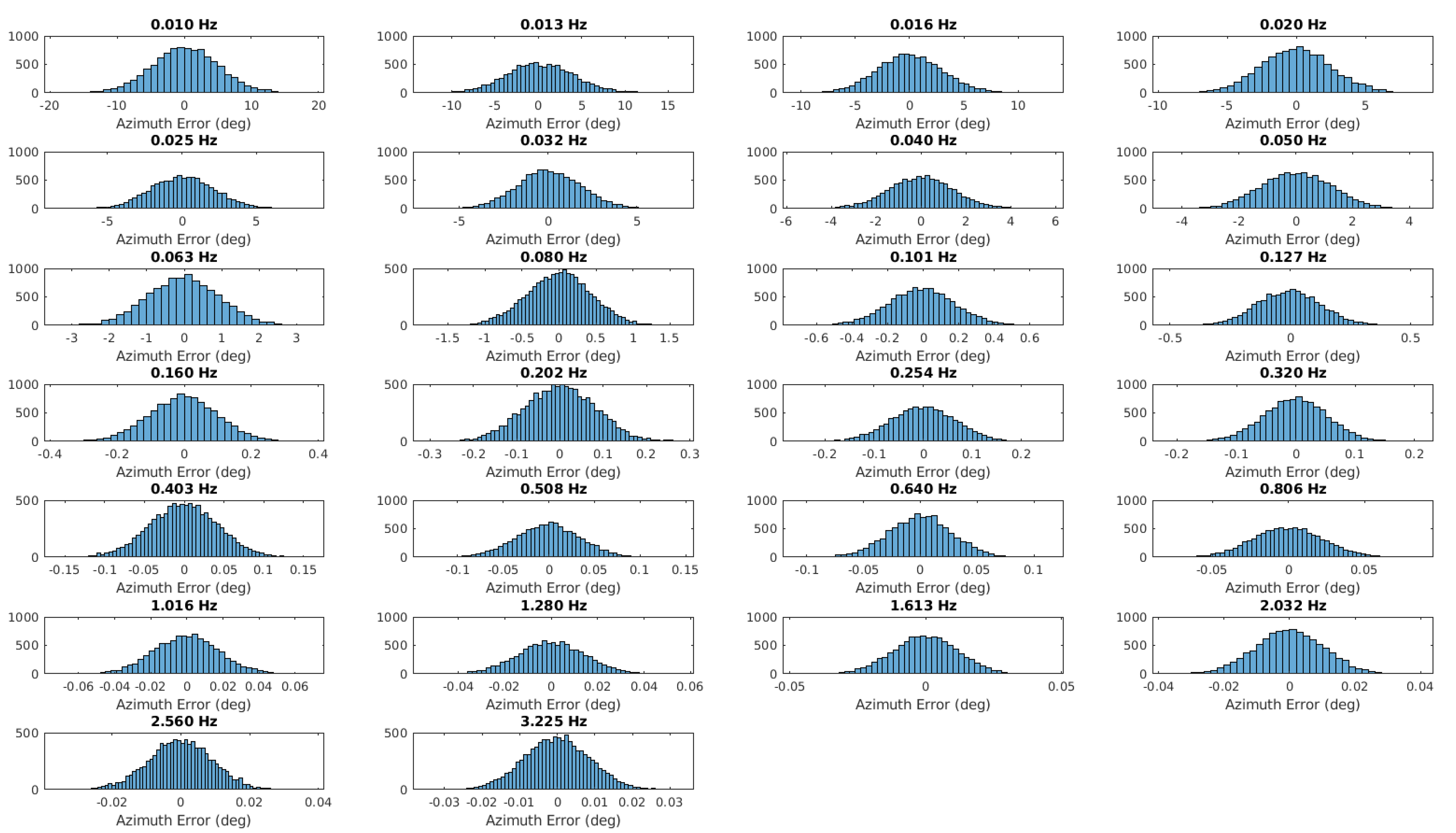
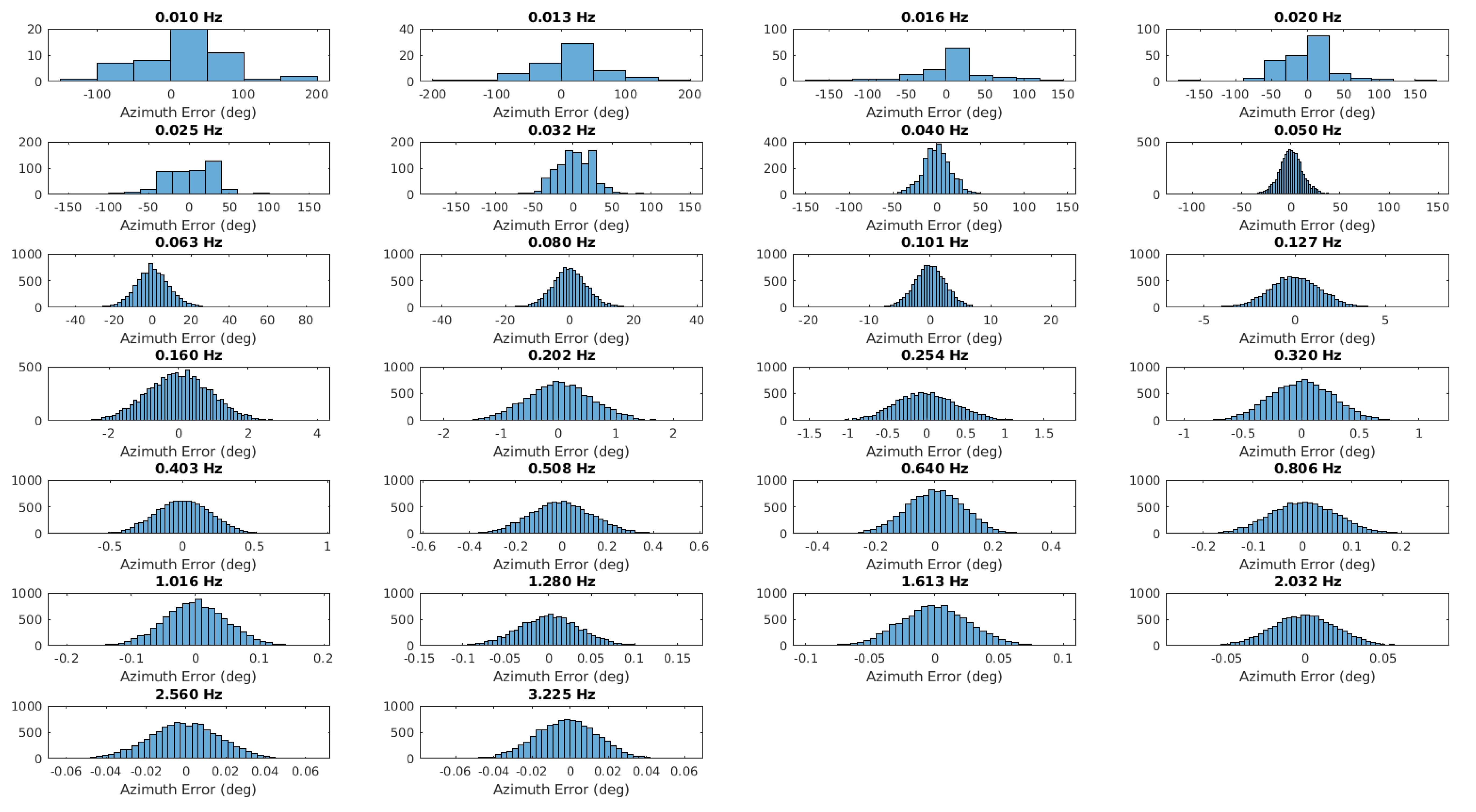
Appendix B.1. Back Azimuth

Figure A1. Back azimuth error (bias), SNR = Inf, M = 10 4 .
Remotesensing 15 01892 g0a1

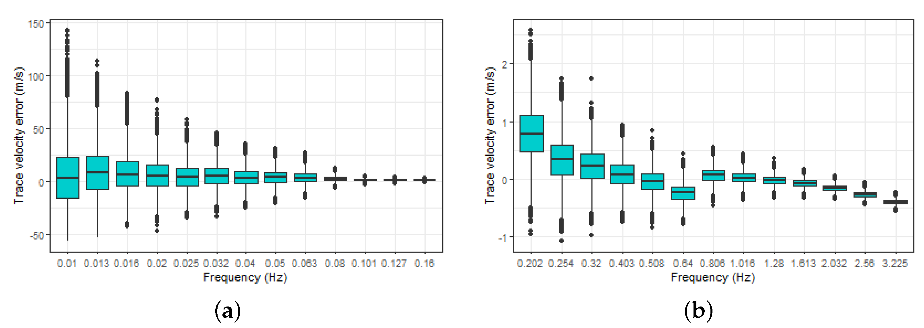
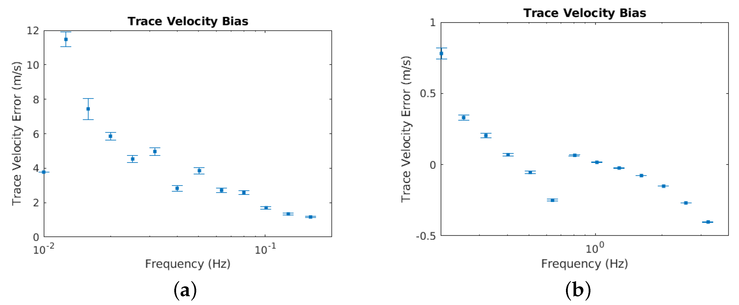
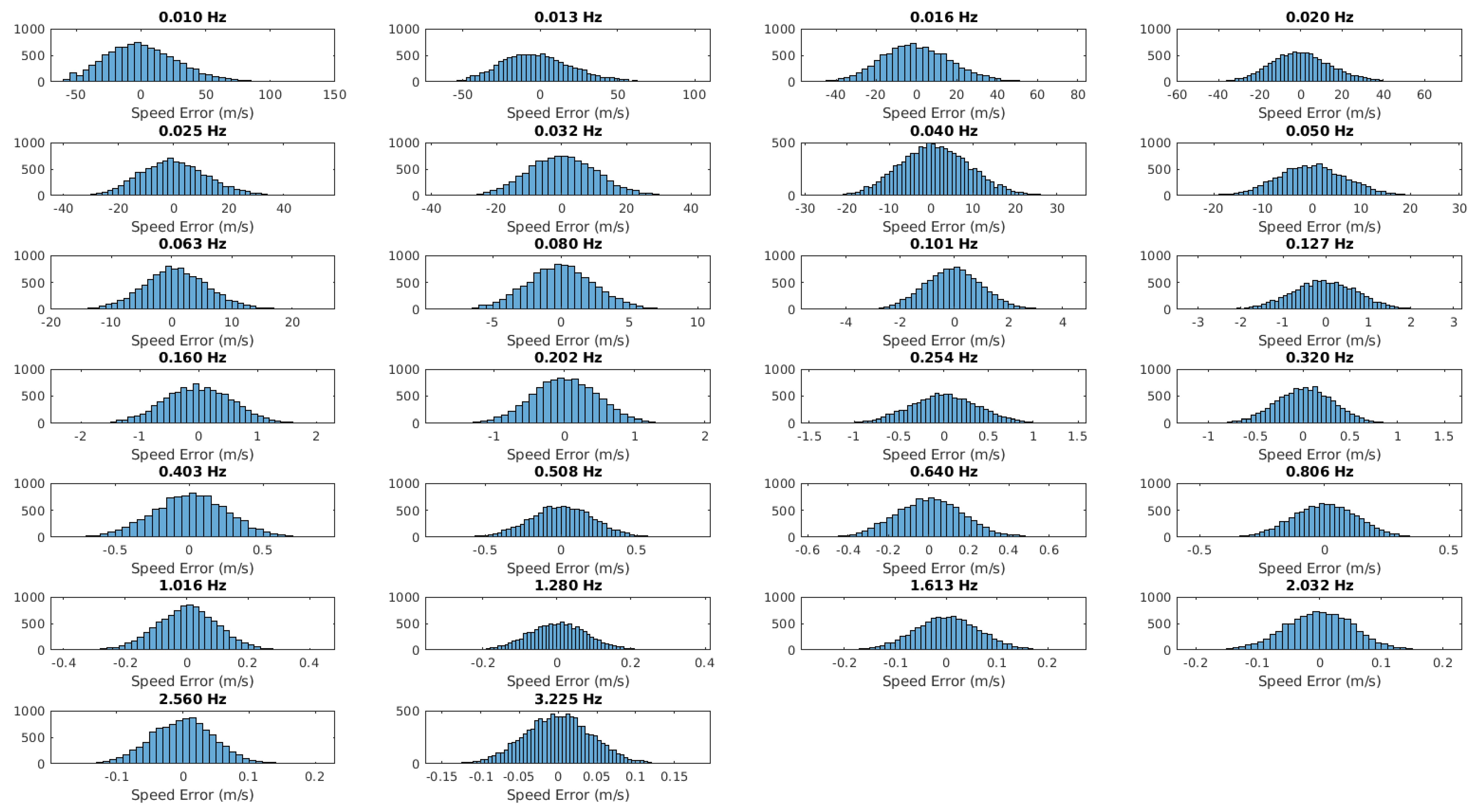
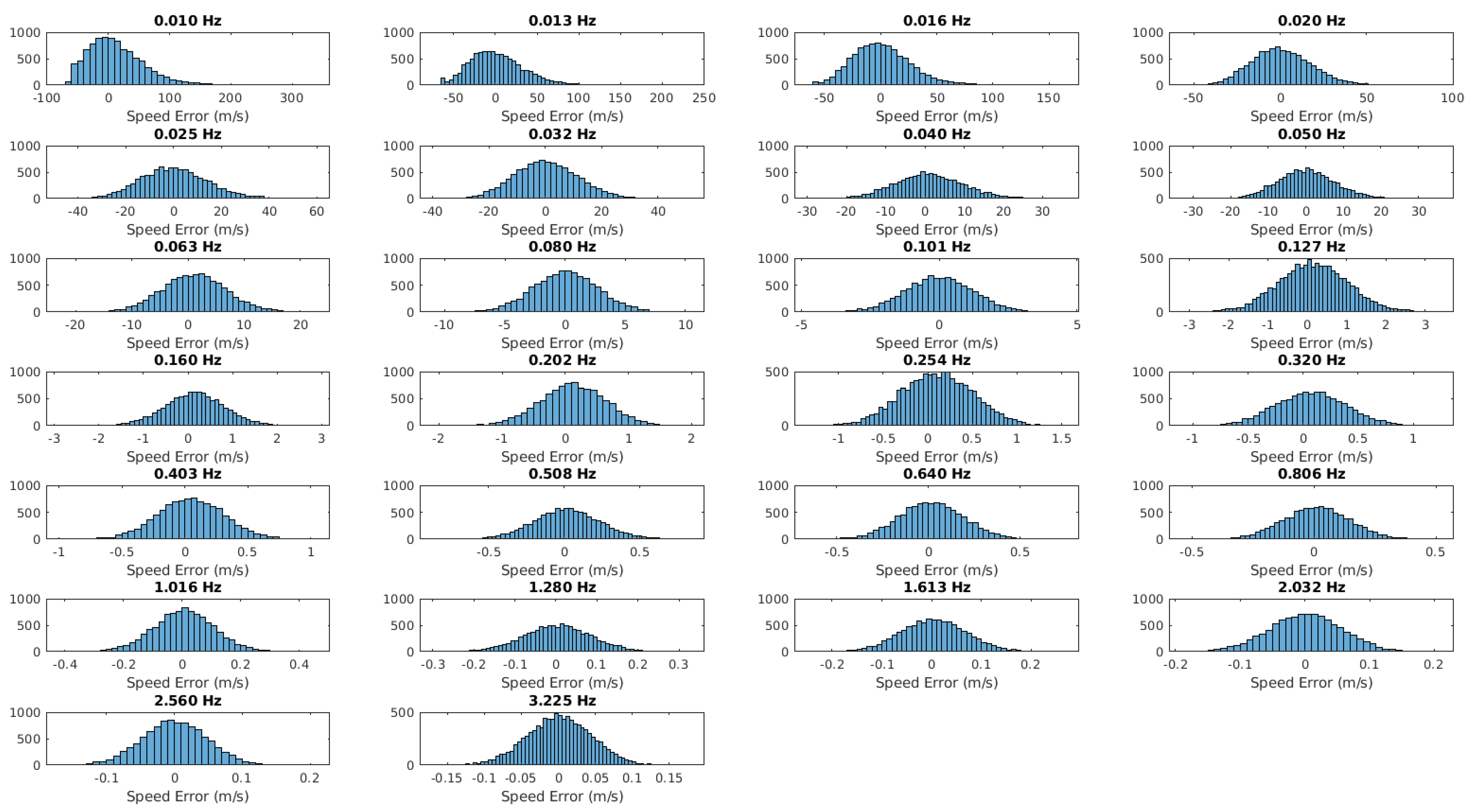
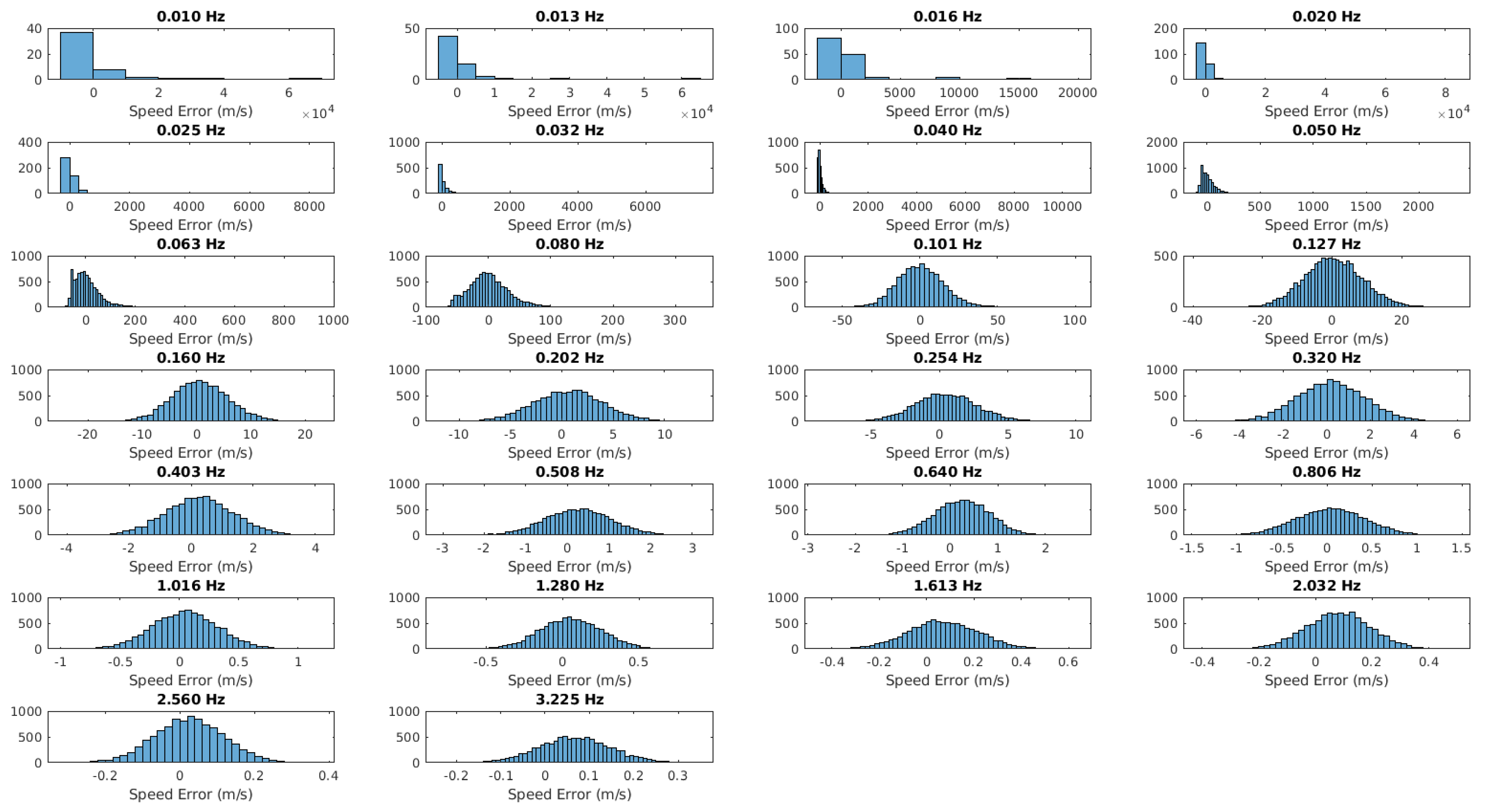
Appendix B.2. Trace Velocity

Figure A2. Trace velocity error (bias), SNR = Inf, M = 10 4 .
Remotesensing 15 01892 g0a2

Appendix C. Results with SNR = 20 dB

Appendix C.1. Back Azimuth

Figure A3. Back azimuth error (bias), SNR = 20 dB, M = 10 4 .
Remotesensing 15 01892 g0a3

Appendix C.2. Trace Velocity

Figure A4. Trace velocity error (bias), SNR = 20 dB, M = 10 4 .
Remotesensing 15 01892 g0a4

Appendix D. Results with SNR = 0 dB

Appendix D.1. Back Azimuth

Figure A5. Back azimuth error (bias), SNR = 0 dB, M = 10 4 .
Remotesensing 15 01892 g0a5

Appendix D.2. Trace Velocity

Figure A6. Trace velocity error (bias), SNR = 0 dB, M = 10 4 .
Remotesensing 15 01892 g0a6

References

  1. Murayama, T.; Kanao, M.; Yamamoto, M.Y.; Ishihara, Y.; Matsushima, T.; Kakinami, Y. Infrasound array observations in the Lützow-Holm Bay region, East Antarctica. Polar Sci. 2015, 9, 35–50. [Google Scholar] [CrossRef]
  2. Evers, L.G.; Haak, H.W. The Characteristics of Infrasound, its Propagation and Some Early History. In Infrasound Monitoring for Atmospheric Studies; Le Pichon, A., Blanc, E., Hauchecorne, A., Eds.; Springer: Dordrecht, The Netherlands, 2009; pp. 3–27. [Google Scholar] [CrossRef]
  3. de Groot-Hedlin, C.; Hedlin, M. Detection of Infrasound Signals and Sources Using a Dense Seismic Network. In Infrasound Monitoring for Atmospheric Studies: Challenges in Middle Atmosphere Dynamics and Societal Benefits; Le Pichon, A., Blanc, E., Hauchecorne, A., Eds.; Springer International Publishing: Cham, Switzerland, 2019; pp. 669–700. [Google Scholar] [CrossRef]
  4. Waxler, R.; Assink, J. Propagation Modeling Through Realistic Atmosphere and Benchmarking. In Infrasound Monitoring for Atmospheric Studies: Challenges in Middle Atmosphere Dynamics and Societal Benefits; Le Pichon, A., Blanc, E., Hauchecorne, A., Eds.; Springer International Publishing: Cham, Switzerland, 2019; pp. 509–549. [Google Scholar] [CrossRef]
  5. Matoza, R.; Le Pichon, A.; Vergoz, J.; Herry, P.; Lalande, J.M.; Lee, H.i.; Che, I.Y.; Rybin, A. Infrasonic observations of the June 2009 Sarychev Peak eruption, Kuril Islands: Implications for infrasonic monitoring of remote explosive volcanism. J. Volcanol. Geotherm. Res. 2011, 200, 35–48. [Google Scholar] [CrossRef] [Green Version]
  6. Freret-Lorgeril, V.; Bonadonna, C.; Corradini, S.; Donnadieu, F.; Guerrieri, L.; Lacanna, G.; Marzano, F.S.; Mereu, L.; Merucci, L.; Ripepe, M.; et al. Examples of Multi-Sensor Determination of Eruptive Source Parameters of Explosive Events at Mount Etna. Remote Sens. 2021, 13, 2097. [Google Scholar] [CrossRef]
  7. De Angelis, S.; Diaz-Moreno, A.; Zuccarello, L. Recent Developments and Applications of Acoustic Infrasound to Monitor Volcanic Emissions. Remote Sens. 2019, 11, 1302. [Google Scholar] [CrossRef] [Green Version]
  8. Campus, P.; Christie, D.R. Worldwide Observations of Infrasonic Waves. In Infrasound Monitoring for Atmospheric Studies; Le Pichon, A., Blanc, E., Hauchecorne, A., Eds.; Springer: Dordrecht, The Netherlands, 2009; pp. 185–234. [Google Scholar] [CrossRef]
  9. Marty, J. The IMS Infrasound Network: Current Status and Technological Developments. In Infrasound Monitoring for Atmospheric Studies; Le Pichon, A., Blanc, E., Hauchecorne, A., Eds.; Springer: Cham, Switzerland, 2019; Chapter 1. [Google Scholar] [CrossRef]
  10. Hupe, P.; Ceranna, L.; Le Pichon, A.; Matoza, R.S.; Mialle, P. International Monitoring System infrasound data products for atmospheric studies and civilian applications. Earth Syst. Sci. Data Discuss. 2022, 2022, 1–40. [Google Scholar] [CrossRef]
  11. Brachet, N.; Brown, D.; Le Bras, R.; Cansi, Y.; Mialle, P.; Coyne, J. Monitoring the Earth’s Atmosphere with the Global IMS Infrasound Network. In Infrasound Monitoring for Atmospheric Studies; Le Pichon, A., Blanc, E., Hauchecorne, A., Eds.; Springer: Dordrecht, The Netherlands, 2009; pp. 77–118. [Google Scholar] [CrossRef]
  12. Cansi, Y. An automatic seismic event processing for detection and location: The P.M.C.C. Method. Geophys. Res. Lett. 1995, 22, 1021–1024. [Google Scholar] [CrossRef]
  13. Cansi, Y.; Klinger, Y. An automated data processing method for mini-arrays. News Lett 1997, 11. [Google Scholar]
  14. Cansi, Y.; Le Pichon, A. Infrasound Event Detection Using the Progressive Multi-Channel Correlation Algorithm. In Handbook of Signal Processing in Acoustics; Havelock, D., Kuwano, S., Vorländer, M., Eds.; Springer: New York, NY, USA, 2008; pp. 1425–1435. [Google Scholar] [CrossRef]
  15. Smart, E.; Flinn, E.A. Fast Frequency-Wavenumber Analysis and Fisher Signal Detection in Real-Time Infrasonic Array Data Processing. Geophys. J. Int. 1971, 26, 279–284. [Google Scholar] [CrossRef] [Green Version]
  16. Evers, L.G.; Haak, H.W. Listening to sounds from an exploding meteor and oceanic waves. Geophys. Res. Lett. 2001, 28, 41–44. [Google Scholar] [CrossRef]
  17. Poste, B.; Charbit, M.; Pichon, A.L.; Listowski, C.; Roueff, F.; Vergoz, J. The Multi-Channel Maximum-Likelihood (MCML) method: A new approach for infrasound detection and wave parameter estimation. In Proceedings of the EGU General Assembly, Vienna, Austria, 23–27 May 2022. [Google Scholar] [CrossRef]
  18. Charbit, M.; abed meraim, K.; Blanchet, G.; Le Pichon, A.; Cansi, Y. OLS vs. WLS for DOA Estimation Based on TDOA Estimates: Application to Infrasonic Signals. In Proceedings of the EGU General Assembly, Vienna, Austria, 23–27 May 2012; p. 7410. [Google Scholar]
  19. Castañeda, N.; Charbit, M.; Moulines, É. Source Localization from Quantized Time of Arrival Measurements. In Proceedings of the 2006 IEEE International Conference on Acoustics Speech and Signal Processing Proceedings, Toulouse, France, 14–19 May 2006; Volume 4, pp. 933–936. [Google Scholar]
  20. Szuberla, C.A.L.; Olson, J.V. Uncertainties associated with parameter estimation in atmospheric infrasound arrays. J. Acoust. Soc. Am. 2004, 115, 253–258. [Google Scholar] [CrossRef]
  21. Bishop, J.W.; Fee, D.; Szuberla, C.A.L. Improved infrasound array processing with robust estimators. Geophys. J. Int. 2020, 221, 2058–2074. [Google Scholar] [CrossRef]
  22. De Angelis, S.; Haney, M.; Lyons, J.; Wech, A.; Fee, D.; Díaz Moreno, A.; Zuccarello, L. Uncertainty in Detection of Volcanic Activity Using Infrasound Arrays: Examples From Mt. Etna, Italy. Front. Earth Sci. 2020, 8, 169. [Google Scholar] [CrossRef]
  23. Norris, D.; Gibson, R.; Bongiovanni, K. Numerical Methods to Model Infrasonic Propagation Through Realistic Specifications of the Atmosphere. In Infrasound Monitoring for Atmospheric Studies; Le Pichon, A., Blanc, E., Hauchecorne, A., Eds.; Springer: Dordrecht, The Netherlands, 2009; pp. 541–573. [Google Scholar] [CrossRef]
  24. Kulichkov, S. On the Prospects for Acoustic Sounding of the Fine Structure of the Middle Atmosphere. In Infrasound Monitoring for Atmospheric Studies; Le Pichon, A., Blanc, E., Hauchecorne, A., Eds.; Springer: Dordrecht, The Netherlands, 2009; pp. 511–540. [Google Scholar] [CrossRef]
  25. Wang, R.; Yi, X.; Yu, L.; Zhang, C.; Wang, T.; Zhang, X. Infrasound Source Localization of Distributed Stations Using Sparse Bayesian Learning and Bayesian Information Fusion. Remote Sens. 2022, 14, 3181. [Google Scholar] [CrossRef]
  26. Garcés, M.A.; Hansen, R.A.; Lindquist, K.G. Traveltimes for infrasonic waves propagating in a stratified atmosphere. Geophys. J. Int. 1998, 135, 255–263. [Google Scholar] [CrossRef] [Green Version]
  27. Assink, J.; Smets, P.; Marcillo, O.; Weemstra, C.; Lalande, J.M.; Waxler, R.; Evers, L. Advances in Infrasonic Remote Sensing Methods. In Infrasound Monitoring for Atmospheric Studies: Challenges in Middle Atmosphere Dynamics and Societal Benefits; Le Pichon, A., Blanc, E., Hauchecorne, A., Eds.; Springer International Publishing: Cham, Switzerland, 2019; pp. 605–632. [Google Scholar] [CrossRef]
  28. Kristoffersen, S.K.; Le Pichon, A.; Hupe, P.; Matoza, R.S. Updated global reference models of broadband coherent infrasound signals for atmospheric studies and civilian applications. Earth Space Sci. 2022, 9. [Google Scholar] [CrossRef]
  29. Walker, K.T.; Hedlin, M.A. A Review of Wind-Noise Reduction Methodologies. In Infrasound Monitoring for Atmospheric Studies; Le Pichon, A., Blanc, E., Hauchecorne, A., Eds.; Springer: Dordrecht, The Netherlands, 2009; pp. 141–182. [Google Scholar] [CrossRef]
  30. Alcoverro, B.; Le Pichon, A. Design and optimization of a noise reduction system for infrasonic measurements using elements with low acoustic impedance. J. Acoust. Soc. Am. 2005, 117, 1717–1727. [Google Scholar] [CrossRef]
  31. Gabrielson, T.B. In situ calibration of atmospheric-infrasound sensors including the effects of wind-noise-reduction pipe systems. J. Acoust. Soc. Am. 2011, 130, 1154–1163. [Google Scholar] [CrossRef]
  32. Raspet, R.; Abbott, J.P.; Webster, J.; Yu, J.; Talmadge, C.; Alberts II, K.; Collier, S.; Noble, J. New Systems for Wind Noise Reduction for Infrasonic Measurements. In Infrasound Monitoring for Atmospheric Studies: Challenges in Middle Atmosphere Dynamics and Societal Benefits; Le Pichon, A., Blanc, E., Hauchecorne, A., Eds.; Springer International Publishing: Cham, Switzerland, 2019; pp. 91–124. [Google Scholar] [CrossRef]
  33. Alcoverro, B. The Design and Performance of Infrasound Noise-Reducing Pipe Arrays. In Handbook of Signal Processing in Acoustics; Havelock, D., Kuwano, S., Vorländer, M., Eds.; Springer: New York, NY, USA, 2008; pp. 1473–1486. [Google Scholar] [CrossRef]
  34. Daniels, F.B. Noise-Reducing Line Microphone for Frequencies below 1 cps. J. Acoust. Soc. Am. 1959, 31, 529–531. [Google Scholar] [CrossRef]
  35. Christie, D.R.; Kennett, B.L.; Tarlowski, C. Advances in infrasound technology with application to nuclear explosion monitoring. In Proceedings of the 29th Monitoring Research Review: Ground-Based Nuclear Explosion Monitoring Technologies, Denver, CO, USA, 25–27 September 2007; Los Alamos National Laboratory: Los Alamos, NM, USA, 2007; pp. 825–835. [Google Scholar]
  36. Green, D.N.; Nippress, A.; Bowers, D.; Selby, N.D. Identifying suitable time periods for infrasound measurement system response estimation using across-array coherence. Geophys. J. Int. 2021, 226, 1159–1173. [Google Scholar] [CrossRef]
  37. Kim, T.S.; Hayward, C.; Stump, B. Local infrasound signals from the Tokachi-Oki earthquake. Geophys. Res. Lett. 2004, 31, 20. [Google Scholar] [CrossRef]
  38. Fee, D.; Macpherson, K.; Gabrielson, T. Characterizing Infrasound Station Frequency Response Using Large Earthquakes and Colocated Seismometers. Bull. Seismol. Soc. Am. 2023. [Google Scholar] [CrossRef]
  39. Wave, S. MB3a Analog Infrasound Sensor Datasheet. 2022. Available online: http://seismowave.com/wp-content/uploads/2019/07/datasheet-MB3a-V2022.2.pdf (accessed on 18 March 2023).
  40. Nief, G.; Talmadge, C.; Rothman, J.; Gabrielson, T. New Generations of Infrasound Sensors: Technological Developments and Calibration. In Infrasound Monitoring for Atmospheric Studies: Challenges in Middle Atmosphere Dynamics and Societal Benefits; Le Pichon, A., Blanc, E., Hauchecorne, A., Eds.; Springer International Publishing: Cham, Switzerland, 2019; pp. 63–89. [Google Scholar] [CrossRef]
  41. Esward, T.; Eichstädt, S.; Smith, I.; Bruns, T.; Davis, P.; Harris, P. Estimating dynamic mechanical quantities and their associated uncertainties: Application guidance. Metrologia 2019, 56, 015002. [Google Scholar] [CrossRef]
  42. Husebye, E.S. Direct measurement of dT/dΔ. Bull. Seismol. Soc. Am. 1969, 59, 717–727. [Google Scholar] [CrossRef]
  43. Mykkeltveit, S.; Ringdal, F.; Kværna, T.; Alewine, R.W. Application of regional arrays in seismic verification research. Bull. Seismol. Soc. Am. 1990, 80, 1777–1800. [Google Scholar] [CrossRef]
  44. Cansi, Y.; Plantet, J.L.; Massinon, B. Earthquake location applied to a mini-array: K-spectrum versus correlation method. Geophys. Res. Lett. 1993, 20, 1819–1822. [Google Scholar] [CrossRef]
  45. Runco, A.; Louthain, J.; Clauter, D. Optimizing the PMCC Algorithm for Infrasound and Seismic Nuclear Treaty Monitoring. Open J. Acoust. 2014, 04, 204–213. [Google Scholar] [CrossRef] [Green Version]
  46. Park, J.; Hayward, C.T.; Zeiler, C.P.; Arrowsmith, S.J.; Stump, B.W. Assessment of Infrasound Detectors Based on Analyst Review, Environmental Effects, and Detection Characteristics. Bull. Seismol. Soc. Am. 2017, 107, 674–690. [Google Scholar] [CrossRef]
  47. Robert, C.; Casella, G. Monte Carlo Statistical Methods; Springer Verlag: Berlin/Heidelberg, Germany, 2004. [Google Scholar]
  48. Rubinstein, R.; Kroese, D. Simulation and the Monte Carlo Method, 3rd ed.; Wiley Series in Probability and Statistics; Wiley: Hoboken, NJ, USA, 2016. [Google Scholar]
  49. ISO 16269-4:2010; Statistical Interpretation of Data—Part 4: Detection and Treatment of Outliers. ISO: Geneva, Switzerland, 2010.
Figure 1. Flowchart of the methodology of uncertainty propagation in the frequency domain with the main uncertainty sources having an effect on the back azimuth and trace velocity of an infrasound wave. In this graph, W and W M C denote, respectively, a QoI and its Monte Carlo estimator.
Remotesensing 15 01892 g001
Figure 2. Example of TDOA outputs arrays for consistency, back azimuth, and trace velocity for a broadband white noise signal, which is filtered between 0.5 and 4 Hz, with a back azimuth of 30° and a trace velocity of 340.3 m/s.
Remotesensing 15 01892 g002
Figure 3. Third-octave frequency bands (y-axis) and corresponding window lengths (x-axis) used by TDOA for this study.
Remotesensing 15 01892 g003
Figure 4. Ishikawa diagram for back azimuth and trace velocity. The red circles indicate the quantifiable uncertainty sources that are considered in this work.
Remotesensing 15 01892 g004
Figure 5. MB2005 response curves. The top panels show the amplitude response (in dB V/Pa) and the bottom panels shows the phase (degrees). The left panels show the absolute results, and the right panels show deviations relative to the average results. The average response is the blue line with the expanded uncertainty being the shaded area.
Remotesensing 15 01892 g005
Figure 6. Calibrated gain of an 18 m WNRS. Top panel is the amplitude of the gain and the bottom panel is the phase of the gain in degrees. For each frequency, the mean and standard deviations (vertical interval) are represented. The red bars highlight the point at approximately 0.08 Hz, which denotes the frequency at which the dip artifact ceases.
Remotesensing 15 01892 g006
Figure 7. The same as Figure 6 but for a defective WNRS with one-quarter of the inlets blocked.
Remotesensing 15 01892 g007
Figure 8. Calibrated gain of an 18 m WNRS + MB3. Top panel is the amplitude of the gain, and the bottom panel is the phase of the gain in degrees. For each frequency, the mean and standard deviations (vertical interval) are represented.
Remotesensing 15 01892 g008
Figure 9. Plots of the six array geometries used in this study.
Remotesensing 15 01892 g009
Figure 10. Back azimuth error (bias) resulting from the estimation method and the uncertainty propagation. The box contains 75 % of the Monte Carlo sampled values for back azimuth error and the error bars range from the lower fence to the upper fence (see [49] for the definition of boxplots). (a) Frequency lower than 0.2 Hz. (b) Frequency higher than 0.2 Hz.
Remotesensing 15 01892 g010
Figure 11. The same as Figure 10, for the trace velocity error (bias). (a) Frequency lower than 0.2 Hz. (b) Frequency higher than 0.2 Hz.
Remotesensing 15 01892 g011
Figure 12. Back azimuth error (bias) due to filtering in TDOA. The error bars represent the standard deviation of the back azimuth errors. (a) Frequency lower than 0.2 Hz. (b) Frequency higher than 0.2 Hz.
Remotesensing 15 01892 g012
Figure 13. Trace velocity error (bias) due to filtering in TDOA. The error bars represent the standard deviation of the trace velocity errors. (a) Frequency lower than 0.2 Hz. (b) Frequency higher than 0.2 Hz.
Remotesensing 15 01892 g013
Figure 14. Plots (log-scales) of the absolute values of the (a) back azimuth and (b) trace velocity mean errors (bias) (points) and standard deviations (dashed lines) as functions of frequency for the microbarometer. The colors represent the different noise levels; blue is infinite SNR (no noise), red is an SNR of 20 dB, and black is 0 dB. The triangles denote the negative errors.
Remotesensing 15 01892 g014
Figure 15. The same as Figure 14, but for the sensor. (a) back azimuth and (b) trace velocity.
Remotesensing 15 01892 g015
Figure 16. Plots (log-scales) of the (a) back azimuth and (b) trace velocity RMSE. The solid lines are the results of the MB2005, and the dashed lines are for the sensor (microbarometer and WNRS). The colors represent different noise levels; blue is infinite SNR, red is 20 dB, and green is 0 dB.
Remotesensing 15 01892 g016
Figure 17. Plots (log-scales) of the (a) back azimuth and (b) trace velocity RMSE as functions of frequency. The OHP station is blue, IS22 is cyan, IS26 is red, IS37 is green, IS27 is magenta, and OHP3 is black.
Remotesensing 15 01892 g017
Figure 18. Plots (log-scales) of the (a) back azimuth and (b) trace velocity mean absolute errors (points) and standard deviations (dashed lines) as functions of frequency, for the case with one defective WNRS. The colors represent the different noise levels; blue is infinite SNR (no noise), red is an SNR of 20 dB, and green is 0 dB. The triangles denote the negative errors.
Remotesensing 15 01892 g018
Figure 19. The color plot (a) shows the back azimuth RMSE for a case with no noise, and a consistency threshold of 0.1 s, as a function of frequency and sensor phase error. The color is the back azimuth RMSE using a log scale. The panel to the right (b) is the median back azimuth RMSE over all sensor phase errors, which is essentially the RMSE for a phase error of 5°; hence, the RMSE is observed at the IMS acceptable limit for the sensor response. The bottom plot (c) is the median RMSE over all frequencies, thus showing the dependency of the RMSE on the sensor phase error.
Remotesensing 15 01892 g019
Figure 20. The same as Figure 19 but for trace velocity. (a) RMSE for a case with no noise, and a consistency threshold of 0.1 s, as a function of frequency and sensor phase error, (b) median RMSE over all sensor phase errors, (c) median RMSE over all frequencies.
Remotesensing 15 01892 g020
Figure 21. The same as Figure 19 but with an SNR of 10 dB. (a) RMSE for a case with no noise, and a consistency threshold of 0.1 s, as a function of frequency and sensor phase error, (b) median RMSE over all sensor phase errors, (c) median RMSE over all frequencies.
Remotesensing 15 01892 g021
Figure 22. The same as Figure 20 but with an SNR of 10 dB. (a) RMSE for a case with no noise, and a consistency threshold of 0.1 s, as a function of frequency and sensor phase error, (b) median RMSE over all sensor phase errors, (c) median RMSE over all frequencies.
Remotesensing 15 01892 g022
Disclaimer/Publisher’s Note: The statements, opinions and data contained in all publications are solely those of the individual author(s) and contributor(s) and not of MDPI and/or the editor(s). MDPI and/or the editor(s) disclaim responsibility for any injury to people or property resulting from any ideas, methods, instructions or products referred to in the content.

