A Single Array Approach for Infrasound Signal Discrimination from Quarry Blasts via Machine Learning

Abstract

Since various phenomena produce infrasound, including both man-made and natural sources, the ever-growing dataflow demands automatic processes via machine learning for signal classification. In this study, we demonstrate a single array approach at the Piszkés-tető (PSZI) infrasound array. Our dataset contains nearly 14,000 manually categorized infrasound detections, processed with the progressive multi channel correlation (PMCC) algorithm from three different sources, such as quarry blasts, storms and signals from a power plant. The dataset was split into a training, a validation and a test subset. Time and frequency domain features as well as PMCC-related features were extracted. Three additional PMCC-related features were constructed in a way to measure the similarity between detections and to be used in single array monitoring. Two different classifiers, support vector machine and random forest, were used for training. Training was performed with three-fold cross validation with grid search. The classifiers were tuned on the training and validation set using the f1 metric (harmonic mean of positive predictive value and true positive rate). Training, validation and testing were performed with and without our three new features that measure similarity between the detections in order to assess their importance in single array monitoring. The selected classifiers reached f1 scores between 0.88 and 0.93. Our results show a promising step toward automatic infrasound event classification.

1. Introduction

Infrasound is known as very low-frequency acoustic wave in the 0.01–20 Hz frequency range. The source of infrasound can be of either natural origin (e.g., microbaroms, bolides, volcanos, and storms) or anthropogenic (e.g., quarry blasts, power plants, and supersonic flights). Since the Comprehensive Nuclear-Test-Ban Treaty (CTBT) was opened for signature in 1996, 53 of 60 planned infrasound stations have been installed worldwide as a component of the International Monitoring System (IMS). In addition, national networks operate permanent and temporary infrasound arrays. In Europe, much of the infrasound related atmospheric research was coordinated by the ARISE project [1,2], and more recently the Central and Eastern European Infrasound Network project [3] contributed to the European Infrasound Bulletin [4].

The ever-growing data volume demands automatic signal processing and classification. When dealing with infrasound signals, classification usually requires ground truth information. For example, this could be seismic data for earthquakes or quarry blasts (e.g., [5,6,7,8]), visual observation for bolides (e.g., [9]) or meteorological data for associating infrasound detections to storms and lightnings (e.g., [10,11,12]). Although the waveform correlation method [13,14,15] is a powerful tool for event association in seismology, it can hardly be used for infrasound waveforms due to the rapid changes in the atmosphere. Hence, infrasound waveforms may look very different from event to event [16,17]. The idea behind automatic infrasound signal classification is that the source mechanism is unique for each kind of event [18]. So even when the signals are changed due to propagation, a set of time domain but mostly frequency domain features can be extracted which are specific for each event type and less dependent on propagation effects.

Machine learning (ML) has been proven to be powerful in different fields of everyday life and science. In infrasound research, it has been used for nuclear reactor monitoring [19], predicting transmission loss due to propagation [20] and signal classification. In the past 20 years there have been different approaches to apply ML models to classify infrasound signals from different kinds of events.

A large set of various features has been proposed, and different methods have been used by researchers. Ham and Park [21] extracted the mel-frequency scaled cepstral coefficients with their derivatives from four different kinds of events. On the coefficients, they applied multi-layer feedforward perceptron by backpropagation, radial basis-function networks and a partial least-squares calibration model. The raw data were collected from five different locations with four different array geometries. Chilo et al. [22] compared three feature extraction methods, the discrete wavelet transform (DWT), the time scale spectrum using continuous wavelet transforms and the mel-frequency scaled cepstral coefficients and their derivatives. On the extracted features, neural networks, logistic regression and support vector machine (SVM) models were trained and tested. A new, different feature extraction method was proposed by Liu et al. [23] by using the Hilbert–Huang transform [24]. The Hilbert–Huang transform performed on each instantaneous mode function derived by empiric mode decomposition and the features were extracted from the marginal spectrum. A SVM classifier was trained and tested on the dataset, which included 45 signals from volcanoes, 42 from tsunamis and 45 from earthquakes, recorded at different IMS stations. On the same dataset, Li et al. [25] tested three types of entropies as features that resulted in somewhat lower accuracy but faster runtime compared to DWT. Albert and Linville [18] used frequency and time domain features as well as normalized power spectra in SVM and convolutional neural network models on a subset of the Infrasound Reference Event Database.

The studies highlighted above represent the state-of-the-art methodologies. They achieved a high variety of accuracy (the number of correctly classified events compared to the number of all events in the test set) from 55% to 100%. The size of the datasets was relatively small, comprising a total of 100–1000 events. It is worth pointing out that the models were robust in the sense that they were trained and tested with data from different stations.

In this paper, we discriminate infrasound signals originating from quarry blasts, storms and a power plant, recorded at a single infrasound array. Our main objective is to build at least a one magnitude larger dataset to demonstrate with high confidence that machine learning models can indeed be used in infrasound signal classification. Our dataset for training, validation and testing consists of approximately 14,000 events, a significantly larger number of events than those used in previous studies. We extracted both time and frequency domain features recommended by the state-of-the-art studies. In addition, we also defined new features and tested their validity. We trained our machine learning discrimination algorithm using SVM and random forest models to demonstrate that they can be successfully applied in infrasound signal classification.

2. Materials and Methods

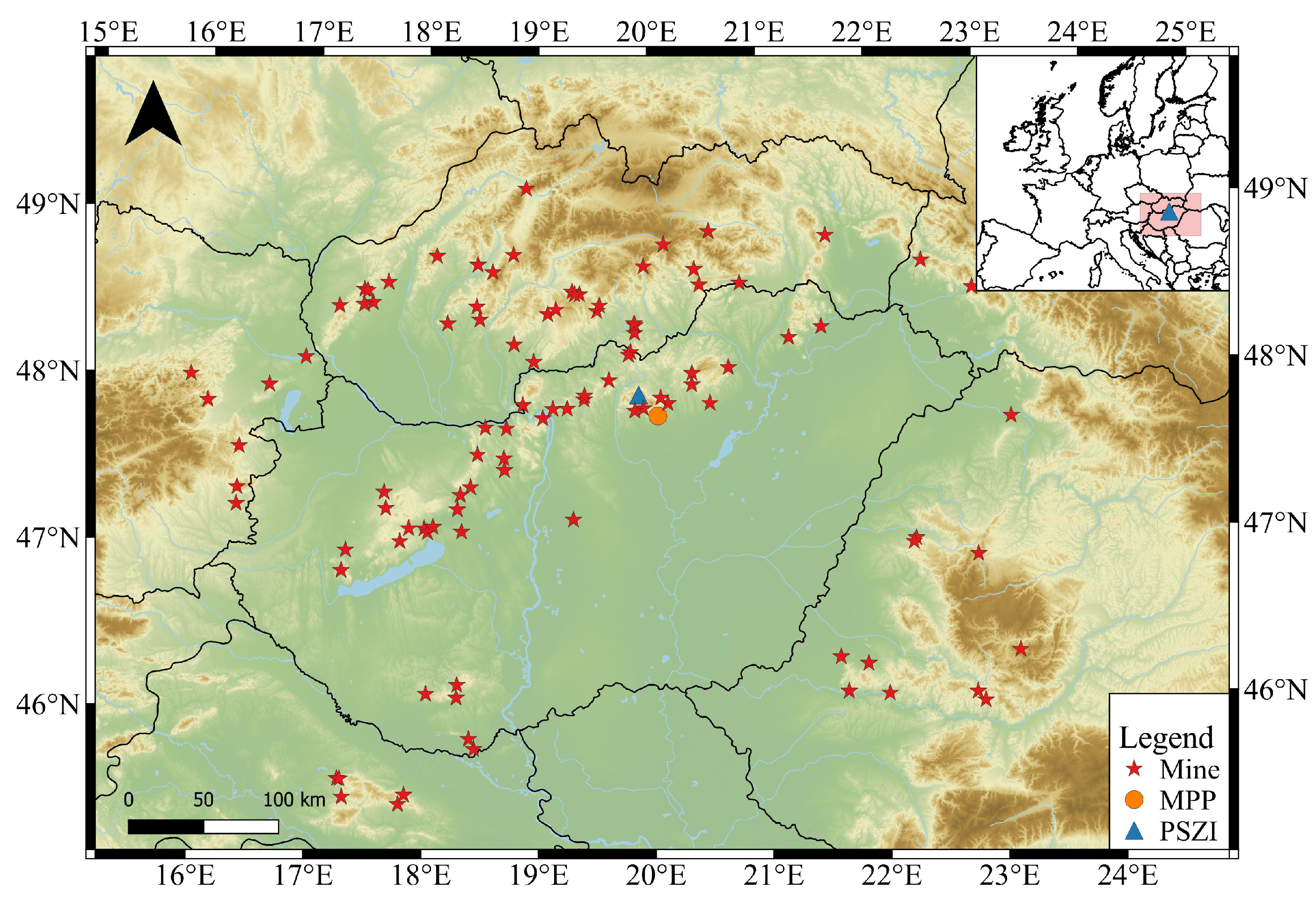
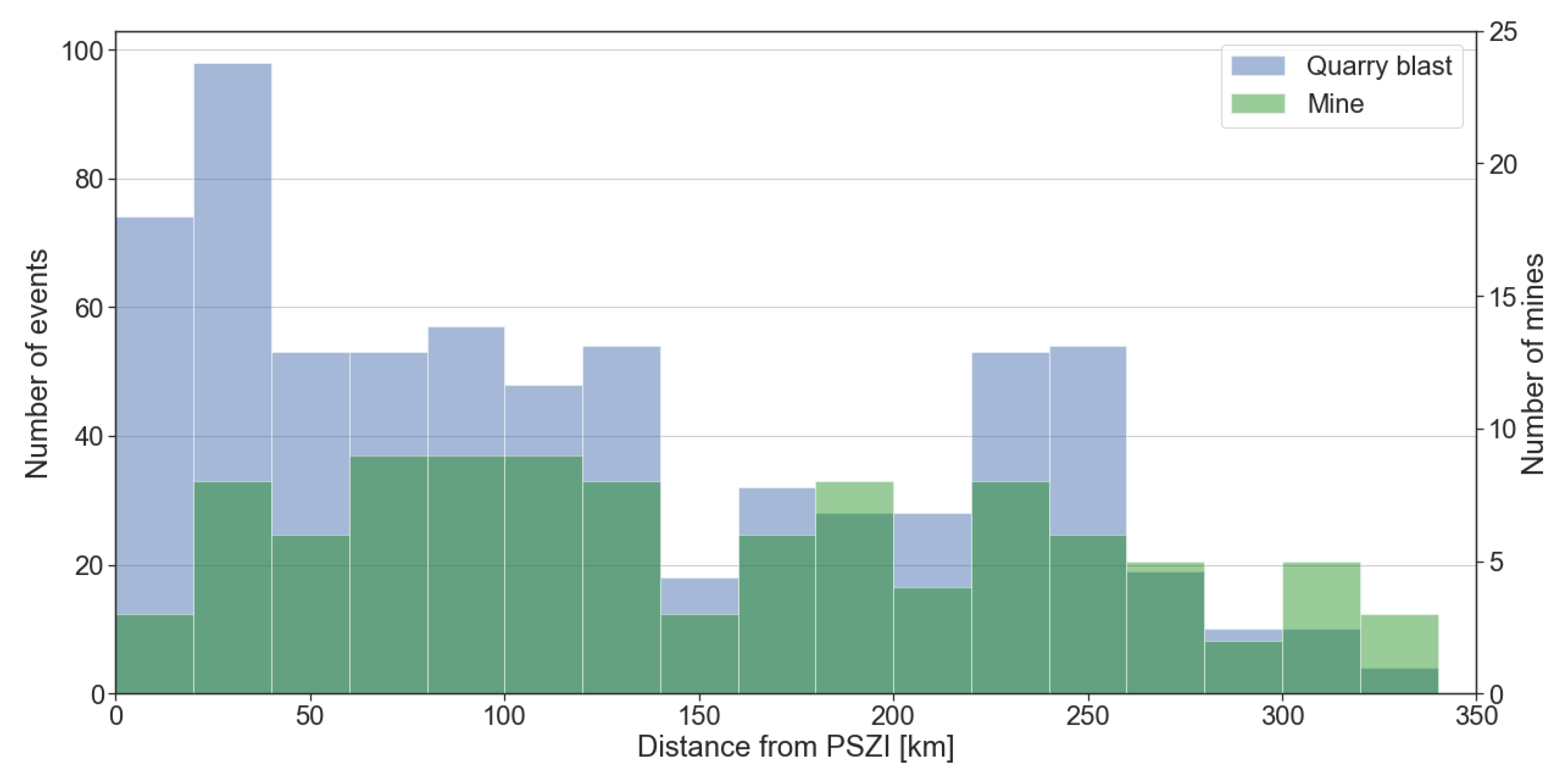
2.1. Data

The infrasound array in Hungary has been operational at Piszkés-tető (PSZI) as part of the Hungarian National Infrasound Network [26], ARISE [1] and Central and Eastern European Infrasound Network [3] collaborations since May 2017. Since then, it has collected approximately a million infrasound detections. The array consists of four SeismoWave MB3d microbarometers with 100 Hz sampling frequency. The aperture is about 250 m, and all instruments are located in a forested area. The central element (PSZI1) of the array is co-located with a seismological station, PSZ, operated by ELKH Kövesligethy Radó Seismological Observatory and the GFZ German Research Center for Geosciences.

For routine data processing, the progressive multi-channel cross correlation (PMCC, [27]) algorithm is used. Infrasound detections are analyzed with the DTK-PMCC and DTK-DIVA processing software that are part of the CTBTO NDC-in-a-box software package. Hereafter, a detection will refer to a PMCC detection. PSZI regularly detects infrasound from microbaroms from the Northern Atlantic [3,28], supersonic flights, bolides [29,30], storms and lightnings [31,32] and quarry blasts [8,33,34,35,36]. The Mátra Power Plant (MPP) at Visonta at about 139° azimuth and at 20 km distance is considered the most dominant coherent noise source near PSZI.

Supervised ML models require labeled datasets for training and testing. For this study, three kinds of event signals from quarry blasts, storms and MPP were classified manually. Detections originated from quarry blasts were taken from the Hungarian Seismo-acoustic Bulletin (HSAB). HSAB has been published annually since 2019, containing several hundreds of quarry blasts events each year [8,33,34,35,36] and is available at http://infrasound.hu (16 March 2023) in IASPEI Seismic Format (ISF). Quarry blasts are relocated using both seismic and infrasound data with iLoc, a further developed version of the single-event location algorithm implemented at the International Seismological Center [37].

Figure 1 shows the active mines and quarries, MPP and PSZI in our region of interest. Figure 2 shows the distributions of quarry blasts and quarries as a function of distance from PSZI. The 695 quarry blasts were detected from 102 different quarries and mines. PSZI is located in an active mining area, and hence a high number of close quarry blasts have been registered. The closest quarry blast in the dataset is 4 km, the farthest is 334 km away from the array, and the mean distance value is 122.5 km. The drop in the number of events at around 140 km can be explained by the geometrical shadow zone, which is consistent with the findings of Czanik et al. [8]. They reported that the geometrical shadow zone for PSZI is in the typical range between 90 and 190 km between tropospheric and stratospheric phases. Nevertheless, shadow zones are not as well defined as those for seismic waves traveling in the Earth’s interior. Owing to the dynamic nature of the atmosphere, under specific conditions, atmospheric ducts may exist that allow for infrasound detections at PSZI, even if the source of the signal falls in the geometrical shadow zone.

Nearly 32,000 infrasound detections were associated to storms at PSZI in earlier studies [31,32]. Note that multiple detections belong to a single storm. Storms were searched for in the time–azimuth domain using DTK-DIVA. The idea was that storms appear as linear features of varying length on the time–azimuth diagrams as they move in time. After collecting the detections into several bulletins, they were compared to lightning distribution from the Blitzortung [38] database as ground truth information. Association was determined on time and space correlation between the detections and the lightning distribution. Spatially, those lightnings were used which fell within $\pm {10}^{°}$ of the azimuthal range defined by the detection list. In time, those lightnings were used which fell within $\pm 10$ minutes of the time interval determined by the first and last detection in the bulletin. Note that the lightning detection times were shifted by the travel time from their location to the infrasound array, with the assumption of direct wave propagation. Additionally, note that in this study, storm class includes everything that comes with storms, e.g., signals from lightnings, turbulence, and vortices [39].

Signals from MPP were classified on a statistical basis and manually. In total, 695 quarry blasts, 32,000 storms and 7615 MPP infrasound detections were labeled. The list of the manually classified detections can be found in the supplementary file, and the waveforms are available at the Geofon website [26].

2.2. Pre-Processing

The input for the feature extraction and ML model training pipeline was an infrasound detection determined by PMCC. For each event, waveforms were cut for the interval of the detection. Prior to the feature extraction, pre-processing was performed on the waveforms. We applied a bandpass filter between 1 and 10 Hz. The lower limit was set to filter out the very low frequency content of the microbaroms considered as noise in this study. The upper limit was driven by the cut off frequency of the instruments used at the array. After filtering, in order to increase the signal-to-noise ratio, beamforming was performed. Delay-and-sum beams were created for each event using the available three or four waveforms.

Note that our dataset of detections is imbalanced in the sense that there are many more available detections associated with storms and MPP than with quarry blasts. Hence, downsampling and the widely used ML technique augmentation were applied. We downsampled the storm detections to reduce the size of the storm set. To minimize the effects of propagation, detections from storms up to 335 km distance were selected, which corresponds to the farthest quarry blast event in the dataset. This way, the number of events labeled as storms was decreased to 5665. To increase the size of the quarry blast sample in the training set, we augmented the quarry blast signals. Augmentation is the process where from the original data a new sample is created [40] through applying transformation or a set of transformations with random parameters and random probability on an instance of a class. Augmentation is a good way to increase the dataset without changing its statistical characteristics. It also helps the model to generalize better and helps against overfitting. For instance, in the case of images, augmentation could represent operations such as random clipping, zooming in or out, rotating, adding noise, and masking. For audio signals, augmentation could be adding noise, time stretch, random gain, polarity change, time, and frequency domain masking. In this study, random Gaussian noise, random time shift, time and frequency masking were applied for all 284 quarry blasts in the training set to make their numbers comparable to the number of storm and MPP detections. Adding random noise to the waveforms means the modulation within a minimum and maximum amplification factor. Applying time shift results in shifting a part of the signal within a range given as a fraction of the total sound length. The time domain mask sets the amplitude values to zero in the signal within a range given as a fraction of the signal length. The frequency domain mask sets the frequency values to zero on the power spectrogram within a given minimum and maximum fraction of the frequency range. For the parameters used please see

Table 1. Transformation parameters used for augmentation.

Transformation	Parameter Range	Probability
Gaussian noise	0.01–0.05	0.5
Time shift	0.0–0.3	1
Time domain mask	0.0–0.03	1
Frequency domain mask	0.0–0.03	1

.

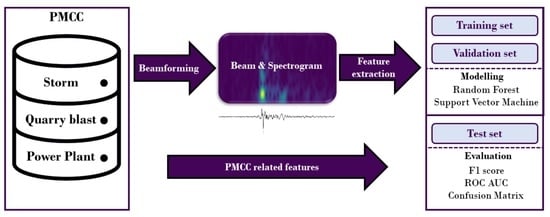
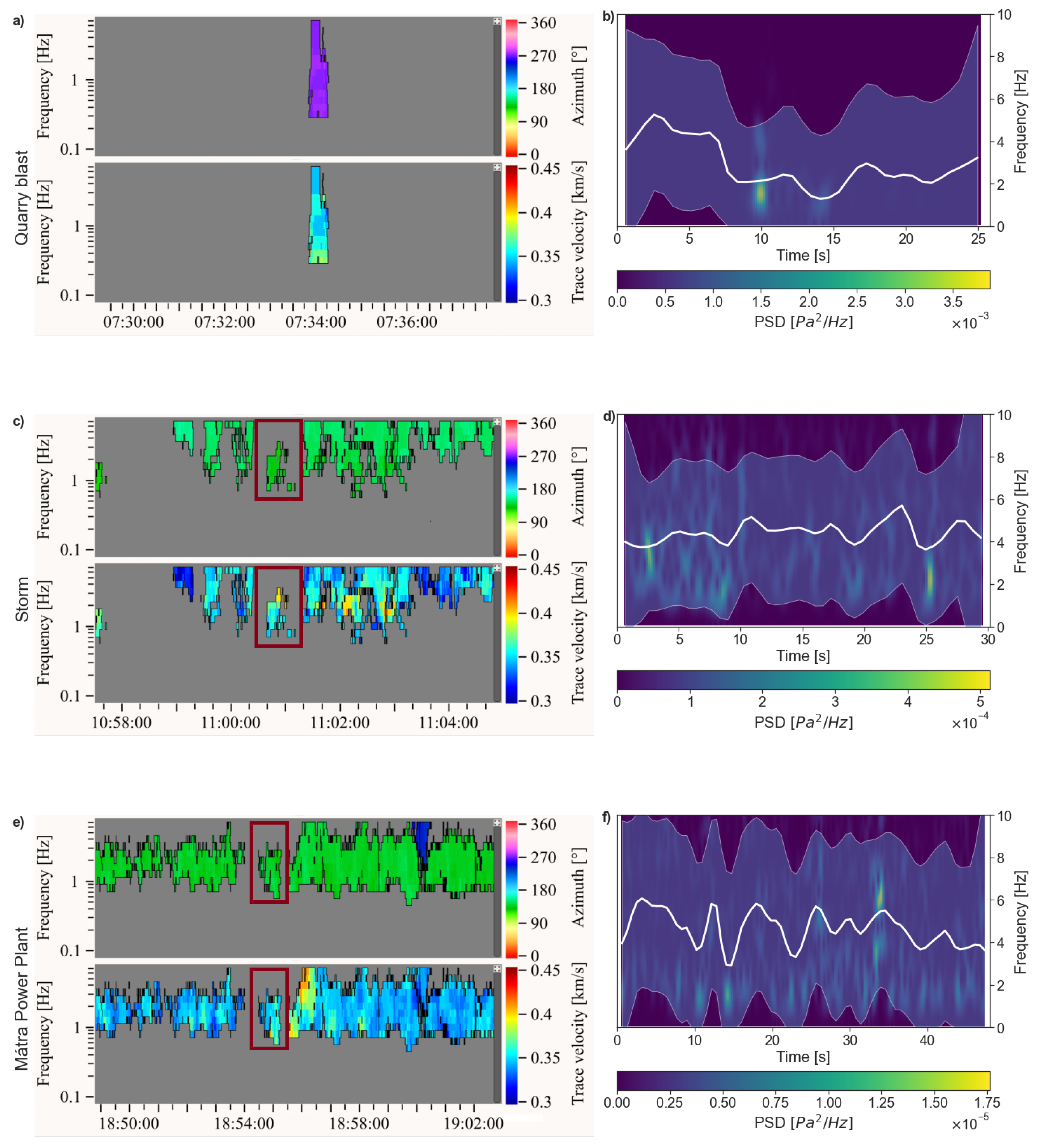
2.3. Feature Extraction

After pre-processing, basically three types of features were extracted; time domain, frequency domain and PMCC-related features. The purpose of time domain and frequency domain features is to describe physical properties of the signals, whereas PMCC-related features include metadata and features that measure similarity between neighboring detections.

We used three time domain features, the number of zero crossings, the signal-to-noise ratio (SNR, here defined as the fraction of the mean and the standard deviation of the amplitude values) and the root mean squared energy ($E_{RMS}$). Even though the number of zero crossings in the signal is computed in the time domain, this feature carries information on a fundamental frequency present in the signal. Let $A_i$ denote the i-th amplitude value in the signal and K the number of points, and then SNR here is defined by

$$\mathrm{SNR}=\frac{\frac{1}{K}{\displaystyle \sum _{k=0}^K}{A}_i}{\sqrt{\frac{{\displaystyle \sum _{k=0}^K}{(A_i-\overline{A_i})}^2}{K}}},$$

(1)

where $\overline{A_i}$ is the mean of the amplitudes. With the denotions used above, the $E_{RMS}$ can be computed by the following equation:

$$E_{RMS}=\sqrt{\frac{1}{K}\sum _{k=0}^K{A}_i^2}$$

(2)

Among the frequency domain features, four were derived from the power spectrograms: the spectral centroid, the spectral bandwidth, the spectral rolloff and the spectral band energy ratio. The spectral centroid is the weighted mean of the magnitudes in each frame of the spectrograms, describing the dominant frequency in the signal as a function of time. The spectral centroid in the i-th frame of spectrogram ($S{C}_i$) can be calculated with the following equation [41]:

$$S{C}_i=\frac{{\displaystyle \sum _{n=1}^N}{S}_i\left(n\right)·n}{{\displaystyle \sum _{n=1}^N}{S}_i\left(n\right)},$$

(3)

here $S_i\left(n\right)$ is the magnitude of the spectrogram in the i-th frame at frequency bin n and N is the number of frames. Spectral bandwidth is the variance or spread around the spectral centroid, and thus it indicates the important frequency range. Similarly to the spectral centroid, the spectral bandwidth in the i-th frame of spectrogram is defined by the following equation with the same denotations [41]:

$$B{W}_i=\frac{{\displaystyle \sum _{n=1}^N}|n-S{C}_i|·S_i\left(n\right)}{{\displaystyle \sum _{n=1}^N}{S}_i\left(n\right)}$$

(4)

The spectral rolloff defines the frequency bin at which a certain percentage of energy (in our case 80% ) is cumulated. The band energy ratio measures the presence of the lower frequencies compared to the higher ones, given by the following equation using $S_i\left(n\right)$ as above [41]:

$${BER}_i=\frac{{\displaystyle \sum _{n=1}^{F-1}}{S}_i{\left(n\right)}^2}{{\displaystyle \sum _{n=F}^N}{S}_i{\left(n\right)}^2},$$

(5)

where F means a predefined frequency value where the split is made. We choose 3 Hz as the split line because analysis of the spectrograms showed that quarry blast events peak below 3 Hz. Figure 3 shows typical detections visualized by DTK-GPMCC and the power spectrograms for the three different sources with two features: the spectral centroid and the spectral bandwidth.

The spectral centroid, spectral bandwidth, spectral rolloff and spectral band energy ratio were calculated in each frame of the spectrogram. This would result in about a 200-element-long feature vector for a 30-s-long beam. For the sake of dimension reduction, median values were derived from these features.

We also extracted two entropy type features, power spectrum entropy (PSE) and singular value decomposition entropy (SVDE), both proposed by Li et al. [25]. PSE is defined as the Shannon entropy of the power spectrum [42]:

$$\mathrm{PSE}=-{\displaystyle \sum _{f=0}^{f_s/2}}S\left(f\right){log}_{2}S\left(f\right),$$

(6)

where $f_s$ is the sampling frequency and $S\left(f\right)$ is the power spectrum. PSE measures how uniform the power spectrum’s distribution is. For a monochromatic signal, PSE is at its minimum and with the presence of more frequency components, the value of the PSE increases [42]. SVDE reflects the dimensionality of the signal. SVDE can be computed in the following way [43,44]. From the signal $[x_1,x_2,\cdots x_N]$ the delay vectors (y(i)) are created:

$$\mathbf{y}\left(i\right)=[x_i,x_{i+\tau },\cdots ,x_{i+(d_E-1)\tau }],$$

(7)

where $\tau$ and $d_E$ denote the delay and the embedding dimension, respectively. In the following step, the embedding space is

$$Y={[\mathbf{y}\left(1\right),\mathbf{y}\left(2\right),\cdots ,\mathbf{y}(N-(d_E-1)\tau )]}^T.$$

(8)

Singular value decomposition is applied on matrix Y to calculate the M number of singular values, ${\sigma }_1,{\sigma }_2,\cdots ,{\sigma }_M$, which compose the singular spectrum. From the singular spectrum, SVDE is given by

$$\mathrm{SVDE}=-{\displaystyle \sum _{i=1}^M}{\overline{\sigma }}_i{log}_2{\overline{\sigma }}_i,$$

(9)

where ${\overline{\sigma }}_1,{\overline{\sigma }}_2,\cdots ,{\overline{\sigma }}_M$ are the normalized singular values in the way that

$${\overline{\sigma }}_i=\frac{{\sigma }_i}{{\displaystyle \sum _{j=1}^M}{\sigma }_j}$$

(10)

From the PMCC result files, the hour of the day and the apparent velocity (horizontal component of the infrasound wave velocity) were taken and used as features. Note that we used hour of the day in UTC, but in Central Europe it still reflects the alternation of days and nights. Furthermore, we defined a three-dimensional box in the time–azimuth–frequency domain in which three features were calculated. The dimensions of the box were $\pm 15$ min $\pm {10}^{°}$ $\pm 1$ Hz wide in each direction for a given detection, respectively. Technically, this means filtering the database that contains all detections with the given parameters. The idea behind this was to measure the similarity between a particular detection and its neighboring detections. The three features are the following:

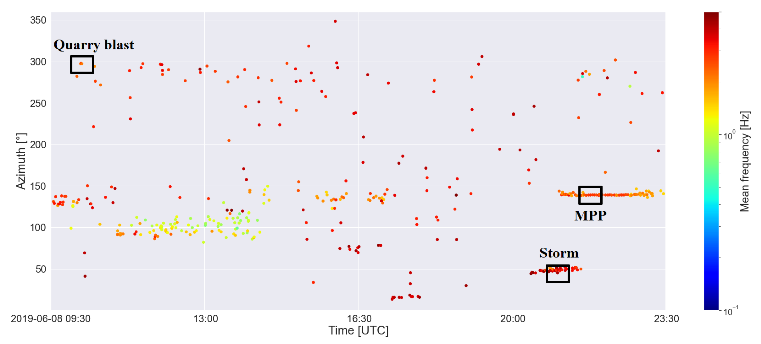
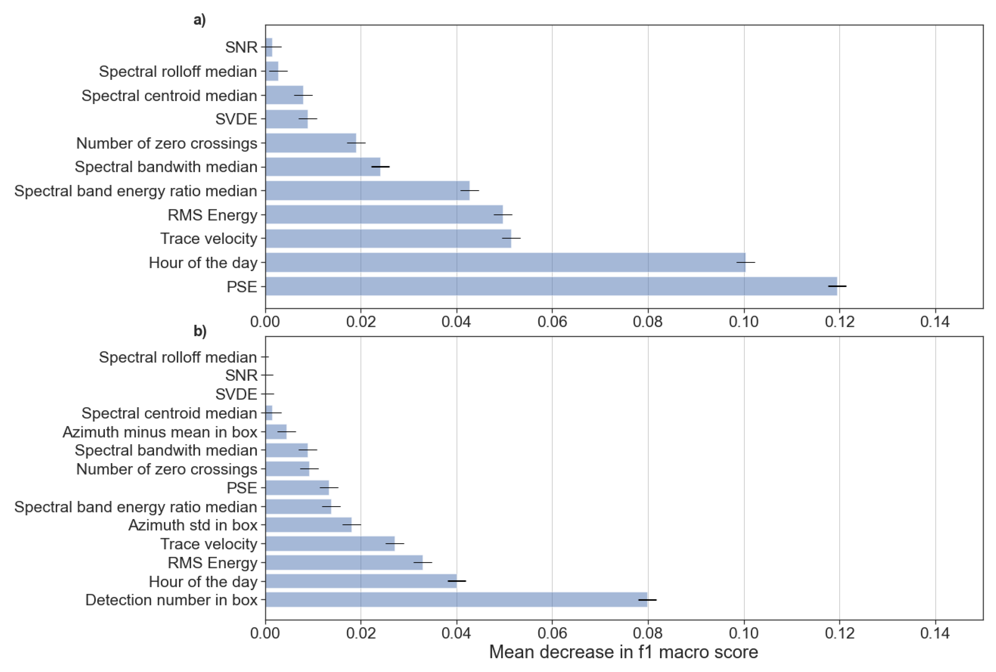
• Number of detections. This feature helps to distinguish between coherent noise sources (e.g., the power plant) and sources when multiple detections belong to the same “event” (e.g., storms) and between, for example, explosions which are usually solitary (or at least have only a few neighbors) on the time–azimuth diagram.
• The difference between the mean azimuth in the box and the detection’s azimuth. For the MPP, almost zero is expected for this value since it is not a moving source. For storms, this feature varies, depending on the movement of the storm relative to the station (visually, the angle on the time–azimuth domain). For quarry blasts, the value also varies. When no neighboring detections are present, basically this feature takes a value of zero, whereas a big difference from the mean is expected when there are adjacent detections.
• The standard deviation of the azimuths in the box. As with the previous feature, we expect larger values for storms and lower ones for MPP. For quarry blasts the same is true as with the foregoing feature.

Figure 4 shows the detections on the time–azimuth diagram, color coded by time, on 8 June 2019 between 09:30 and 23:30 UTC. In this interval, detections from all the three sources can be seen. The black boxes frame one detection from each class in which the three features are calculated. Note that the box is illustrated only in the time–azimuth domain. Additionally, note that the PMCC-derived features are all considered station specific.

With the dimension reduction, 14 element feature vectors were generated. Figure 5 shows the mean and standard deviation of each feature for each class. Note that each feature is normalized with a standard scaler. Even though all three classes follow a similar pattern on the polar plot, a separation can be seen for the detection number in the box from feature between the quarry blasts and the other two classes. The separation is seen both for the mean values and the standard deviation, which implies that this might be an important feature.

2.4. Model Selection

For training, validation and testing, the dataset was split into three parts. The number of events in each subset for the different sources can be found in

Table 2. Distribution of the number of labeled storms, quarry blast and MPP detections among the training, validation and test subsets. The quarry blast events in the training set include the augmented samples. The approximate percentages are present in the brackets.

	Storm	Quarry Blast	MPP
Training	3962 (75%)	568 (58%)	5334 (75%)
Validation	834 (15%)	203 (21%)	1161 (15%)
Test	869 (15%)	208 (21%)	1120 (15%)

. Note that the quarry blast events in the training set also include the augmented samples. The approximate percentages are presented in the brackets. We used a 70%–15%–15% split for the training, validation and test sets, respectively, which is a commonly applied practice to divide a dataset into these three parts [45]. However, due to the low number of quarry blasts, the split percentage for this class is slightly different. The total number of events used in this study is 13,975 plus the 284 augmented quarry blasts in the quarry blast training set. On all subsets, a standard scaler was applied (fit on the training set), meaning that the features were scaled to zero mean and unit variance.

Classification was performed with two fundamentally different classifiers, random forest [46] and support vector machine (SVM) [47]. SVM has been proven to be powerful at infrasound signal classification (e.g., [18,23,25] ), whilst random forests are easy to interpret. These models were also favored since they work well on relatively small datasets. Training was performed without and with the three features that measure the similarity between the detections, resulting in 11- and 14-element-long feature vectors, respectively, to assess their importance in a single array signal classifier.

Even though augmentation and downsampling were performed, the number of quarry blast events was still small compared to the size of the other two classes. Hence, accuracy was not selected as the evaluation metric because this can be misleading when imbalance is present. Instead, we used the f1 score. The f1 score is calculated as the harmonic mean of precision (positive predictive value) and recall (true positive rate). We also computed the area under the receiver operating curve (ROC AUC) scores to evaluate the results. We also generated and analyzed confusion matrices on the validation set. Afterward, the selected random forest and SVM models were tested on the test set. Model training and evaluation was performed via the Sckikit-learn framework [48], a widely used Python library for ML.

Fine tuning of the hyperparameters for both SVM and random forest models was performed by grid search with three-fold cross validation on the training set. For the random forest classifiers, the following hyperparameters were tuned: number of trees, minimum samples per leaf, minimum samples per split, maximum depth, and maximum features. Minimum samples per split gives the minimum number of samples needed to make a split at an internal node. Minimum samples per leaf give the minimum number of samples needed to be present at a leaf node. The maximum feature hyperparameter gives the number of features to consider when looking for the best split, computed from the total number of features. Hyperparameter tuning for the SVM models was mainly about tuning the regularization parameter C. For the kernel, the radial basis function was used. For the kernel coefficient, $\gamma$ both auto and scale were used. In the case of auto, $\gamma =1/n_{features}$, where $n_{features}$ is the number of features (11 or 14 in our case). When the scale is set, $\gamma =1/(n_{features}·var\left(X\right))$, where $var\left(X\right)$ is the variance of the input matrix. For more details, please see the Skickit-learn documentation [48]. We tried different grids; the final ones are presented in

Table 3. Hyperparameter grid for the random forest classifiers.

Parameter	Values
Number of trees	20, 30, 40, 50, 60, 80
Minimum samples per leaf	2, 4, 8, 12, 16, 20, 24
Minimum samples per split	2, 4, 8, 12, 16, 20, 24
Maximum depth	10, 20, 30, 40, 50
Maximum features	all, log2, square root

and

Table 4. Hyperparameter grid for the SVM classifiers.

Parameter	Values
C	1, 2, 3, 4, 5, 10, 20, 50, 100, 200, 500, 1000
kernel	Radial Basis Function
$\gamma$	scale, auto

for the random forest and the SVM classifiers, respectively.

3. Results

Approximately 14,000 previously categorized PMCC detections were processed and used to extract features. Frequency domain, time domain and PMCC-related features were fed into SVM and random forest models, which were trained with three-fold cross-validation using grid search for hyperparameter tuning on the training set. The performance of the models was measured using f1 and ROC AUC scores; in addition, the confusion matrices were analyzed on the test set.

First, training was performed without the three features that measure similarity between the features, i.e., 11 features were used. For this case, Figure 6a,c show the confusion matrices on the test set for the selected random forest and SVM classifiers, respectively. On the test set, the best random forest and SVM models (in the sense of highest number of true positive quarry blasts and f1 score) reached an f1 score of 0.88. For mean cross validation on the training set and validation scores, see

Table 5. Performance of the selected random forest and SVM classifiers.

	Training CV Mean f1 Score	Training CV f1 Score Standard Deviation	Validation f1 Score	Test f1 Score
Random forest with 11 features	0.84	0.009	0.89	0.88
Random forest with 14 features	0.86	0.005	0.92	0.92
SVM with 11 features	0.83	0.016	0.88	0.88
SVM with 14 features	0.88	0.012	0.93	0.93

. After adding the three specific features that measure the similarity between the detections, and training on all the 14 features, we experienced an increase in the f1 and AUC scores, as well as in the number of true positive quarry blast events. On the test set, Figure 6b,d show the confusion matrices for the highest true positive quarry blast event and f1 score achieved by random forest and SVM classifiers, respectively. It should be noted that the largest difference between this and the case above is that the number of correctly identified quarry blasts increased from 162 to 195 (77.9% to 93.8%) and from 169 to 192 (81.2% to 92.3%) for the random forest and SVM models, respectively. On the test set, the random forest model with the lowest number of false positive quarry blasts reached 0.92 f1 score, whereas this number for the SVM model is 0.93. Table 5 contains mean cross validation on the training set and validation scores.

Figure 7 shows the one-versus-all ROC curves generated on the test set, meaning that the classifiers are trained with the parameters determined by the cross validation but in a binary case, e.g., quarry blasts versus signals from MPP plus storms. The upper row contains the results of the random forest classifiers and the lower one the results of SVM. The ROC curves are consistent with the confusion matrices in the sense that storms are less separated from the other classes, especially in the 14-element-long feature vector case (right column). After the addition of the three features that measure the similarity between the detections, the ROC curves moved closer to the upper left corner, indicating a better performance.

4. Discussion

Training, validation and testing were performed without and with the detection number in box, the azimuth minus mean in box and the azimuth standard deviation in box, the three features that measure the similarity between the detections. In both cases, random forest and SVM classifiers were used and compared. Based on the confusion matrices (Figure 6) and on the ROC curves (Figure 7) in both cases, the selected classifiers could distinguish well between the quarry blast events and storm and MPP associated signals. However, when adding the three specific features, the classifiers performed better when it came to differentiating between quarry blasts and the others. The f1 score, measured on the test set, increased from 0.88 to 0.92 in the case of the random forest and to 0.93 in the case of the SVM classifiers. The number of true positive quarry blasts increased from 162 to 195 (77.9% to 93.8%) and from 169 to 192 (81.2% to 92.3%) for the random forest and SVM models, respectively. Thus, single array monitoring might benefit from these three features. In each case, the trained classifiers predicted much more quarry blasts to be storms than signals from MPP. The reason behind this is most likely the method of labeling the detections as storms, due to which the storms class is not as pure as the quarry blast and MPP ones, i.e., more mislabeled detections are in this class than in the other two. Based on the f1 scores, the ROC curves and confusion matrices of both the SVM and random forest models worked well on our dataset.

Our goal was to discriminate detections associated with quarry blasts from the two other classes. The classifiers managed to distinguish quarry blasts and MPP but struggled more with storms. To better interpret these misclassifications, we analyzed the beams and the spectrograms. The detections that were predicted to be quarry blasts originated from 22 different storms. Out of the 22 storms, 14 that were predicted to be quarry blasts were close or just above the array. On their beams, large peaks or pulses are present, which might be associated with lightnings, and thus they look similar to beams from quarry blasts. On the other hand, the waveforms of the quarry blasts predicted as storms are noisy and have higher frequency components than most of the samples in this class. These characteristics are the probable cause for the misidentifications.

For the two selected random forest models, the permutation feature importance was calculated. The permutation feature importance can be derived using trained tree models, randomly swapping two features and measuring, in our case, the f1 score drop. The bigger the drop in the metric, the more important the feature. The process was run 50 times, which was enough to give reliable permutation feature importances. The permutation feature importances can be seen in Figure 8. Where the features that measure similarity between the detections were included (Figure 8b), two of them, the detection number in box and the azimuth standard deviation in box, placed first and fifth, indicating that these two features are behind the improvement of the model’s performance, and they are indeed important and useful in single array monitoring. The azimuth minus mean in box, however, was less important. In both cases, the SNR, spectral rolloff and spectral centroid slid to the last three places. Among the four features derived from the power spectrograms, spectral bandwidth reached the best places. The power spectrum entropy had the greatest role in the 11-feature case but fell back with the addition of the three specific features. Note that in both cases, the hour of the day feature took second place, even though it is a simple feature. Since quarries carry out their explosions at specific times of the day, the discriminating power of the hour of the day feature is somewhat expected, and indeed machine learning has found this feature on its own.

When it comes to infrasound signal classification, the most significant issue is the effect of propagation on the signals. Albert and Linville [18] trained SVM and convolutional neural network (CNN) models on a subset of the Infrasound Reference Event Database (IRED). The signals in the dataset were recorded at IMS stations from all around the world, consisting of 256 signals from mines and quarries, 152 from chemical and accidental explosions, 103 from earthquakes and 104 associated with volcanic activity. The average distances between the source and receiver were 581, 1571, 1199 and 2084 km for the four classes, respectively. Training was performed in a binary case, i.e., earthquakes versus volcanic activity, and with all four classes. Using SVM, in the former case they achieved 75% accuracy and 55% in the latter. These numbers were 74% and 56% for the CNN architectures, respectively. The input for the SVM models were time and frequency domain features. Spectrograms were used to train the CNN classifiers. Prior to training SVM models, they selected eight features based on relative feature importance determined by random forests. The top two among these were distance between the source and receiver, and waveform duration (which increases with distance), suggesting range dependency on infrasound signal classification. The authors tried to identify a range beyond which the misclassification rate highly increases. They found a range for the mines and quarries class only, although they did not quantify it.

In our study, the dataset for training, validation and testing was constructed in such a way that it contains events from a 335 km radius, measured from PSZI. This allows a more local investigation than with the IRED, described above. The MPP is at a fixed location, so only the distance of storms and quarry blasts vary. We did not include the distance between the source and receiver for three reasons. Firstly, for storms, only estimated values could have been given for this feature. Secondly, due to the fixed distance of MPP, the models might have learned that everything at 20 km distance is from the MPP class. Lastly, for unknown events, the distance between the source and receiver is also unknown, so it cannot be used in automatic monitoring. On the other hand, it might be useful to analyze the results. Figure 9 shows the distribution of misclassified quarry blasts as a function of distance in the test set for the four final models. Based on the histograms, no clear dependency can be seen for misclassification as a function of distance in our dataset. The major difference in our study is the more local distance range, where the propagation time is much shorter and therefore there is not enough time for the differences in the features to accumulate. However, range-dependent conditions could also be responsible for particular guiding conditions that would be detrimental to classification in some cases.

Besides the distances, we analyzed the celerities (the average speed along the raypath between source and receiver) of the quarry blasts. Celerities were calculated as a fraction of the known distances and the travel times, given as the difference of the blast times and detection times. In our dataset, based on the celerities, tropospheric (>310 m/s) and stratospheric (280–320 m/s) phases are present [49,50,51]. Figure 10 shows the computed celerities as a function of distance for the training set and for the detections that were misclassified in the test set. Here, each event is plotted, which was misclassified either by the random forest or the SVM model. The high variability below 50 km is due to the errors in the event location. The gap around 140 km is caused by the geometrical shadow zone, from which we only have few detections. Based on the figure, we did not find connection between misclassification and celerities (thus different phases). Previously, we did not find a relation between the distance and the misclassification either. Based on the foregoing, it would be an exaggeration to say that classification is not affected by propagation, but we can say that we have not seen any evidence of it in the local range we examined. Future studies might benefit from features that describe the state of the atmosphere, but such features are indeed difficult to construct for ML.

To be consistent with other studies, we calculated the accuracies (number of correctly classified events divided by the number of all events in the test set), which are 90% and 93% for the random forest models and 91% for the two SVM models, whereas the studies mentioned in the introduction reached accuracies between 55% and 100%. Note that our accuracy values may be affected by the imbalanced sets of events in our dataset. Additionally, note that previous studies used datasets containing 100–1000 events in total. The results on our 1–2 magnitude larger dataset, containing approximately 14,000 detections from three categories in total, imply that ML techniques are powerful at automatic infrasound event discrimination.

Finally, it should be noted that during the dimension reduction, when median values were taken from the features that are calculated in each frame, information loss may have occurred. Thus, a better approach would be to use spectrograms (as applied by Albert and Linville [18] ), and make an automatic feature extraction, e.g., using a CNN. Although deep learning methods require bigger databases, this is our future goal. We plan to add more classes and increase the size of the classes as well. The use of increasingly larger datasets for ML-based infrasound event classification should be necessary for future studies.

5. Conclusions

In this paper, we trained, validated and tested SVM and random forest machine learning models using features extracted from infrasound waveforms and PMCC detections. The dataset contained nearly 14,000 manually categorized infrasound detections from three different sources, such as quarry blasts, storms and signals from the Mátra Power Plant. The performance of the classifiers was measured using the f1 metric; also, the ROC curves and confusion matrices were analyzed. Training was performed, including and excluding three features that measure the similarity between the detections, resulting in 11- and 14-element-long feature vectors, respectively, to retrieve their importance. In the former case, both classifiers carried out an f1 score of 0.88. In the latter case, random forest reached 0.92 and SVM achieved 0.93 f1 scores. Our results show that both the SVM and random forest models are applicable for infrasound signal classification.

To describe the physical properties of the signals, we used time and frequency domain features recommended by previous studies. Based on the permutation feature importances, the SNR, spectral rolloff median and spectral centroid median performed worst, while PSE, RMS energy and spectral band energy ratio median were the best performers. We introduced new, PMCC-derived features in order to measure the similarity between detections. We found that two of these features, the detection number in box and the azimuth standard deviation in box, are highly efficient for event monitoring and discrimination at a single infrasound station. The hour of the day proved to be a powerful feature in the discrimination.

We analyzed the misclassified detections from quarry blasts as a function of celerity and distance, as these are propagation-related features. It cannot be claimed that classification is not affected by propagation, but we did not find a clear correlation between these two propagation features and misclassification in the local range we examined. Future studies might benefit from constructing features that are related to the state of the atmosphere.

The use of a dataset that is at least one magnitude larger than those used in previous studies showed promising results in the field of automatic, ML-based infrasound event classification. However, the compilation and application of even larger datasets which not only contain more detections in each class but have a larger variety of different types of events are required for future studies.

References

1. Blanc, E.; Ceranna, L.; Hauchecorne, A.; Charlton-Perez, A.; Marchetti, E.; Evers, L.G.; Kvaerna, T.; Lastovicka, J.; Eliasson, L.; Crosby, N.B.; et al. Toward an Improved Representation of Middle Atmospheric Dynamics Thanks to the ARISE Project. Surv. Geophys. 2018, 39, 171–225. [Google Scholar] [CrossRef] [Green Version]
2. Blanc, E.; Pol, K.; Le Pichon, A.; Hauchecorne, A.; Keckhut, P.; Baumgarten, G.; Hildebrand, J.; Höffner, J.; Stober, G.; Hibbins, R.; et al. Middle Atmosphere Variability and Model Uncertainties as Investigated in the Framework of the ARISE Project. In Infrasound Monitoring for Atmospheric Studies, 2nd ed.; Le Pichon, A., Blanc, E., Hauchecorne, A., Eds.; Springer: Dordrech, The Netherlands, 2019; pp. 845–888. [Google Scholar]
3. Bondár, I.; Šindelářová, T.; Ghica, D.; Mitterbauer, U.; Liashchuk, A.; Baše, J.; Chum, J.; Czanik, C.; Ionescu, C.; Neagoe, C.; et al. Central and Eastern European Infrasound Network: Contribution to infrasound monitoring. Geophys. J. Int. 2022, 230, 565–579. [Google Scholar] [CrossRef]
4. Pilger, C.; Ceranna, L.; Ross, J.O.; Vergoz, J.; Le Pichon, A.; Brachet, N.; Blanc, E.; Kero, J.; Liszka, L.; Gibbons, S.; et al. The European Infrasound Bulletin. Pure Appl. Geophys. 2018, 175, 3619–3638. [Google Scholar] [CrossRef] [Green Version]
5. Stump, B.W.; Hedlin, M.A.H.; Pearson, D.C.; Hsu, V. Characterization of mining explosions at regional distances: Implications with the International Monitoring System. Rev. Geophys. 2002, 40, 2-1–2-21. [Google Scholar] [CrossRef]
6. Arrowsmith, S.; Hedlin, M.; Stump, B.; Arrowsmith, M. Infrasonic Signals from Large Mining Explosions. Bull. Seismol. Soc. Am. 2008, 98, 768–777. [Google Scholar] [CrossRef]
7. Che, I.Y.; Park, J.; Kim, T.S.; Hayward, C.; Stump, B. On the use of a dense network of seismo-acoustic arrays for near-regional environmental monitoring. In Infrasound Monitoring for Atmospheric Studies, 2nd ed.; Le Pichon, A., Blanc, E., Hauchecorne, A., Eds.; Springer: Dordrecht, The Netrherlands, 2019; pp. 409–448. [Google Scholar]
8. Czanik, C.; Kiszely, M.; Mónus, P.; Süle, B.; Bondár, I. Identification of Quarry Blasts Aided by Infrasound Data. Pure Appl. Geophys. 2021, 178, 2287–2300. [Google Scholar] [CrossRef]
9. Belli, G.; Pace, E.; Marchetti, E. Detection and source parametrization of small-energy fireball events in Western Alps with ground-based infrasonic arrays. Geophys. J. Int. 2021, 225, 1518–1529. [Google Scholar] [CrossRef]
10. Farges, T.; Blanc, E. Characteristics of infrasound from lightning and sprites near thunderstorm areas. J. Geophys. Res. Space Phys. 2010, 115, 1–17. [Google Scholar] [CrossRef] [Green Version]
11. Chum, J.; Diendorfer, G.; Šindelářová, T.; Baše, J.; Hruška, F. Infrasound pulses from lightning and electrostatic field changes: Observation and discussion. J. Geophys. Res. Atmos. 2013, 118, 653–664. [Google Scholar] [CrossRef]
12. Farges, T.; Hupe, P.; Le Pichon, A.; Ceranna, L.; Listowski, C.; Diawara, A. Infrasound Thunder Detections across 15 Years over Ivory Coast: Localization, Propagation, and Link with the Stratospheric Semi-Annual Oscillation. Atmosphere 2021, 12, 1188. [Google Scholar] [CrossRef]
13. Israelsson, H. Correlation of waveforms from closely spaced regional events. Bull. Seismol. Soc. Am. 1990, 80, 2177–2193. [Google Scholar] [CrossRef]
14. Harris, D.B. A waveform correlation method for identifying quarry explosions. Bull. Seismol. Soc. Am. 1991, 81, 2395–2418. [Google Scholar] [CrossRef]
15. Gibbons, S.J.; Ringdal, F. The detection of low magnitude seismic events using array-based waveform correlation. Geophys. J. Int. 2006, 165, 149–166. [Google Scholar] [CrossRef] [Green Version]
16. Kulichkov, S.N. Long-range propagation and scattering of low-frequency sound pulses in the middle atmosphere. Meteorol. Atmos. Phys. 2004, 85, 47–60. [Google Scholar] [CrossRef]
17. Gibbons, S.; Asming, V.; Fedorov, A.; Fyen, J.; Kero, J.; Kozlovskaya, E.; Kvaerna, T.; Liszka, L.; Näsholm, S.P.; Raita, T.; et al. The European Arctic: A Laboratory for Seismoacoustic Studies. Seismol. Res. Lett. 2015, 86, 917–928. [Google Scholar] [CrossRef] [Green Version]
18. Albert, S.; Linville, L. Benchmarking Current and Emerging Approaches to Infrasound Signal Classification. Seismol. Res. Lett. 2020, 91, 921–929. [Google Scholar] [CrossRef]
19. Chai, C.; Ramirez, C.; Maceira, M.; Marcillo, O. Monitoring Operational States of a Nuclear Reactor Using Seismoacoustic Signatures and Machine Learning. Seismol. Res. Lett. 2022, 93, 1660–1672. [Google Scholar] [CrossRef]
20. Brissaud, Q.; Näsholm, S.P.; Turquet, A.; Le Pichon, A. Predicting infrasound transmission loss using deep learning. Geophys. J. Int. 2023, 232, 274–286. [Google Scholar] [CrossRef]
21. Ham F., M.; Park, S. A robust neural network classifier for infrasound events using multiple array data. In Proceedings of the 2002 International Joint Conference on Neural Networks, Honolulu, HI, USA, 12–17 May 2002. [Google Scholar]
22. Chilo, J.; Lindblad, T.; Olsson, R.; Hansen, S. Comparison of Three Feature Extraction Techniques to Distinguish between Different 72 Infrasound Signals. In Progress in Pattern Recognition; Sameer, S., Maneesha, S., Eds.; Springer: London, UK, 2007; pp. 75–82. [Google Scholar]
23. Liu, X.; Li, M.; Tang, W.; Wang, S.; Wu, X. A New Classification Method of Infrasound Events Using Hilbert-Huang Transform and Support Vector Machine. Math. Probl. Eng. 2014, 2014, e456818. [Google Scholar] [CrossRef] [Green Version]
24. Huang, N.E.; Shen, Z.; Long, S.R.; Wu, M.C.; Shih, H.H.; Zheng, Q.; Yen, N.; Tung, C.C.; Liu, H.H. The empirical mode decomposition and the Hilbert spectrum for nonlinear and non-stationary time series analysis. Proc. Math. Phys. Eng. Sci. 1998, 454, 903–995. [Google Scholar] [CrossRef]
25. Li, M.; Liu, X.; Liu, X. Infrasound signal classification based on spectral entropy and support vector machine. Appl. Acoust. 2016, 113, 116–120. [Google Scholar] [CrossRef]
26. Hungarian National Infrasound Network on Geofon Website. Available online: https://geofon.gfz-potsdam.de/waveform/archive/network.php?ncode=HN (accessed on 10 March 2023).
27. Cansi, Y. An automatic seismic event processing for detection and location: The P.M.C.C. Method. Geophys. Res. Lett. 1995, 22, 1021–1024. [Google Scholar] [CrossRef]
28. Šindelářová, T.; De Carlo, M.; Czanik, C.; Ghica, D.; Kozubek, M.; Podolská, K.; Baše, J.; Chum, J.; Mitterbauer, U. Infrasound signature of the post-tropical storm Ophelia at the Central and Eastern European Infrasound Network. J. Atmos. Solar-Terr. Phys. 2021, 217, 105603. [Google Scholar] [CrossRef]
29. Kereszturi, A.; Barta, V.; Bondar, I.; Czanik, C.; Igaz, A.; Monus, P. Connecting ionospheric, optical, infrasound and seismic data from meteors over Hungary. J. Int. Meteor Organ. 2020, 48, 188–192. [Google Scholar]
30. Kereszturi, Á.; Barta, V.; Bondár, I.; Czanik, C.; Igaz, A.; Mónus, P.; Rezes, D.; Szabados, L.; Pál, B.D. Review of synergic meteor observations: Linking the results from cameras, ionosondes, infrasound and seismic detectors. Mon. Notices R. Astron. Soc. 2021, 506, 3629–3640. [Google Scholar] [CrossRef]
31. Pásztor, M.; Czanik, C.; Bondár, I. Exploiting infrasound detections to identify and track regional storms. In Proceedings of the EGU General Assembly Conference Abstracts, Online Conference, 19–30 April 2021. EGU21-6525. [Google Scholar]
32. Pásztor, M.; Czanik, C.; Sindelarova, T.; Chum, J.; Bondár, I. Identifying and tracking regional storms with infrasound data. In Proceedings of the CTBTO Science and Technology Conference Book of Abstracts, Online Conference, 28 June–2 July 2021; p. P2.3-585. [Google Scholar]
33. Bondár, I.; Czanik, C.; Czecze, B.; Kalmár, D.; Kiszely, M.; Mónus, P.; Süle, B. Hungarian Seismo-Acoustic Bulletin, 2017–2018; MTA CSFK GGI-Kövesligethy Radó Seismological Observatory: Budapest, Hugary, 2019. [Google Scholar]
34. Bondár, I.; Czanik, C.; Czecze, B.; Kalmár, D.; Kiszely, M.; Mónus, P.; Pásztor, M.; Süle, B. Hungarian Seismo-Acoustic Bulletin, 2019–2020; MTA CSFK GGI-Kövesligethy Radó Seismological Observatory: Budapest, Hugary, 2020. [Google Scholar]
35. Bondár, I.; Czanik, C.; Czecze, B.; Kalmár, D.; Kiszely, M.; Mónus, P.; Pásztor, M.; Süle, B. Hungarian Seismo-Acoustic Bulletin, 2020–2021; MTA CSFK GGI-Kövesligethy Radó Seismological Observatory: Budapest, Hugary, 2021. [Google Scholar]
36. Bondár, I.; Pásztor, M.; Czanik, C.; Kiszely, M.; Mónus, P.; Süle, B. Hungarian Seismo-Acoustic Bulletin; 2019–2020; Bondár, I., Ed.; Institute for Geological and Geochemical Research, Research Centre for Astronomy and Earth Sciences: Budapest, Hungary; ELKH Budapest and Kövesligethy Radó Seismological Observatory, Institute of Earth Physics and Space Science, ELKH: Sopron, Hungary, 2022. [Google Scholar]
37. Bondár, I.; Storchak, D. Improved location procedures at the International Seismological Centre. Geophys. J. Int. 2011, 186, 1220–1244. [Google Scholar] [CrossRef] [Green Version]
38. Blitzortung. Available online: https://www.blitzortung.org (accessed on 11 March 2023).
39. Bowman, H.S.; Bedard, A.J. Observations of Infrasound and Subsonic Disturbances Related to Severe Weather. Geophys. J. Int. 1971, 26, 215–242. [Google Scholar] [CrossRef]
40. Géron, A. Hands-On Machine Learning with Scikit-Learn, Keras, and TensorFlow, 2nd ed.; Roumeliotis, R., Tache, N., Eds.; O’Reilly Media: North Sepastopol, CA, USA, 2019. [Google Scholar]
41. Krishnamurthi, R.; Dhanalekshmi, G.; Adarsh, K. Chapter 10—Using Wavelet Transformation for Acoustic Signal Processing in Heavy Vehicle Detection and Classification. In Autonomous and Connected Heavy Vehicle Technology; Krishnamurthi, R., Kumar, A., Gill, S.S., Eds.; Academic Press: Cambridge, MA, USA, 2022; pp. 199–209. [Google Scholar] [CrossRef]
42. Inouye, T.; Shinosaki, K.; Sakamoto, H.; Toi, S.; Ukai, S.; Iyama, A.; Katsuda, Y.; Hirano, M. Quantification of EEG Irregularity by Use of the Entropy of the Power Spectrum. Electroencephalogr. Clin. Neurophysiol. 1991, 79, 204–210. [Google Scholar] [CrossRef]
43. Roberts, S.J.; Penny, W.; Rezek, I. Temporal and Spatial Complexity Measures for Electroencephalogram Based Brain-Computer. Med. Biol. Eng. Comput. 1999, 39, 93–98. [Google Scholar] [CrossRef] [PubMed]
44. Bao, F.S.; Liu, X.; Zhang, C. PyEEG: An Open Source Python Module for EEG/MEG Feature Extraction. Comput. Intell. Neurosci. 2011, 2011, 406391. [Google Scholar] [CrossRef] [Green Version]
45. Nguyen, Q.H.; Ly, H.; Ho, L.S.; Al-Ansari, N.; Le, H.V.; Tran, V.Q.; Prakash, I.; Pham, B.T. Influence of Data Splitting on Performance of Machine Learning Models in Prediction of Shear Strength of Soil. Math. Probl. Eng. 2021, 2021, 4832864. [Google Scholar] [CrossRef]
46. Breiman, L. Random Forests. Mach. Learn. 2001, 45, 5–32. [Google Scholar] [CrossRef] [Green Version]
47. Cortes, C.; Vapnik, V. Support-Vector Networks. Mach. Learn. 1995, 20, 273–297. [Google Scholar] [CrossRef]
48. Pedregosa, F.; Varoquaux, G.; Gramfort, A.; Michel, V.; Thirion, B.; Grisel, O.; Blondel, M.; Prettenhofer, P.; Weiss, R.; Dubourg, V.; et al. Scikit-Learn: Machine Learning in Python. J. Mach. Learn. Res. 2011, 12, 2825–2830. [Google Scholar]
49. Kulichkov, S.N. On infrasonic arrivals in the zone of geometric shadow at long distances from surface explosions. In Proceedings of the Ninth Annual Symposium on Long-Range Propagation, Oxford, MS, USA, 14–15 September 2000. [Google Scholar]
50. Negraru, P.T.; Golden, P.; Herrin, E.T. Infrasound Propagation in the “Zone of Silence”. Seismol. Res. Lett. 2010, 81, 614–624. [Google Scholar] [CrossRef]
51. Nippress, A.; Green, N.D.; Marcillo, E.O.; Arrowsmith, J.S. Generating regional infrasound celerity-range models using ground-truth information and the implications for event location. Geophys. J. Int. 2014, 197, 1154–1165. [Google Scholar] [CrossRef] [Green Version]
Figure 1. Map of Hungary and neighboring countries showing PSZI (blue triangle), MPP (orange circle) and known mines and quarries (red stars). The map in the upper right shows an overview of the examined region in Europe.
Remotesensing 15 01657 g001
Figure 2. Distribution of the quarry blasts (blue) and distribution of known mines and quarries (green) as a function of distance measured from PSZI. The high number of close-distance quarry blasts are due to the active mining region near PSZI. The drop in the number of events at 140 km can be explained by the geometrical shadow zone, from which PSZI can detect signals only during specific atmospheric conditions.
Remotesensing 15 01657 g002
Figure 3. Typicaldetections and power spectrograms for quarry blasts, storms and signals from MPP. The left column (a,c,e) shows the detections visualized by DTK-GPMCC, and the right column (b,d,f) contains power spectrograms for each type of events used. In the case of storms and MPP where more detections are present, the selected ones for which the power spectrogram is calculated are marked with a red rectangle. In the left column, detections are plotted in the time–frequency domain using the logarithmic frequency scale. In the upper panels, the detections are color coded by azimuth, whereas they are color coded by trace velocity in the lower ones. In the right column, the spectral centroid is depicted with a white solid line, the shaded area represents the spectral centroid ± spectral bandwidth.
Remotesensing 15 01657 g003
Figure 4. Detections on the time–azimuth diagram, color coded by time, on 8 June 2019 between 09:30 and 23:30 UTC. In this interval detections from a quarry blast (upper left), from MPP (middle right) and from a storm (bottom right) are present. The black boxes frame one detection from each class in which the three features (detection number in box, azimuth standard deviation in box and azimuth minus mean in box) are calculated.
Remotesensing 15 01657 g004
Figure 5. Mean feature values (solid line) and standard deviation (shaded area) for the three classes used. Note that each feature is normalized with a standard scaler.
Remotesensing 15 01657 g005
Figure 6. Confusion matrices for the selected models generated on the test set. The upper row (a,b) contains the results of the random forest classifiers and the lower one (c,d) the ones of SVM. The left column (a,c) represents the case without the three PMCC-derived features and the right column (b,d) shows the confusion matrices with the PMCC-derived features. The percentages in each row sum up to 100%.
Remotesensing 15 01657 g006
Figure 7. One-versus-all ROC curves for the random forest and SVM models generated on the test set. The upper row (a,b) contains the results of the random forest classifiers and the lower one (c,d) the of SVM ones. The left column (a,c) represents the case, when the three features that measures the similarity between detections were excluded (resulting in 11 element-long feature vectors) and the right column (b,d) represents the results with them (resulting in 14 element-long feature vectors). For each one-versus-all classifier, the ROC AUC scores are present in the legend. The black dashed line represents a random classifier. A line reaching the (0,1) point in the top left corner would mean a perfect classifier.
Remotesensing 15 01657 g007
Figure 8. Permutation feature importance for the selected random forest models. The bars represent the mean f1 score decrease in the 50 runs and the black ticks mark the standard deviations. (a) shows when the features that measure the similarity between the detections were excluded (resulting in 11-element-long feature vectors) and (b) shows the case when they were included (resulting in 14-element-long feature vectors).
Remotesensing 15 01657 g008
Figure 9. Distribution of misclassified quarry blasts in the test set as a function of distance measured from PSZI. The upper row (a,b) contains the results of the random forest classifiers and the lower one (c,d) those of SVM. The left column (a,c) represents the case, when the three features that measure the similarity between detections were excluded (resulting in 11-element-long feature vectors) and the right column (b,d) represents the results with them (resulting in 14-element-long feature vectors).
Remotesensing 15 01657 g009
Figure 10. Scatter plot of the celerities as a function of distance measured from PSZI for the quarry blast detections. Detections from the training set are colored by blue, misclassified detections in the test set are orange.
Remotesensing 15 01657 g010