Communication

Basal Melt Patterns around the Deep Ice Core Drilling Site in the Dome A Region from Ice-Penetrating Radar Measurements

1
School of Earth Sciences and Resources, China University of Geosciences, Beijing 100083, China
2
Key Laboratory of Polar Science of Ministry of Natural Resources (MNR), Polar Research Institute of China, Shanghai 200136, China
3
School of Oceanography, Shanghai Jiao Tong University, Shanghai 200030, China
4
Institute for Interdisciplinary and Innovate Research, Xi’an University of Architecture and Technology, Xi’an 710055, China
5
School of Earth and Space Sciences, University of Science and Technology of China, Hefei 230026, China
6
Department of Earth and Space Sciences, Southern University of Science and Technology, Shenzhen 518055, China
*
Author to whom correspondence should be addressed.
Remote Sens. 2023, 15(7), 1726; https://doi.org/10.3390/rs15071726
Submission received: 9 February 2023 / Revised: 9 March 2023 / Accepted: 21 March 2023 / Published: 23 March 2023
(This article belongs to the Section Environmental Remote Sensing)

Abstract

:
Basal melt in the Dome A region will influence the deep-ice-core drilling at Kunlun Station. The melting point (wet bedrock) has a higher reflectivity than the surrounding area, which can be assessed using radar echoes from the bedrock. This paper uses a linear absorption model to determine wet and dry ice–bedrock interfaces around the Kunlun drilling site. In the determination process, an artificial intelligence model was applied to extract the ice–bedrock interface for inferring the ice thickness. Additionally, the various depth-averaged attenuation rates were used to identify the maximal range of basal melting. We mapped the patterns of the wet points on the bottom of the ice sheet and the modeled basal temperature to verify the results of the wet bed conditions. According to these maps of wet bed conditions, the areas with basal melting around the drilling site primarily appear in valley walls with low basal temperatures and are linked with hydraulic potential and bedrock elevation. Identifying the ice–bedrock interface is challenging in the valley bottom area, where the melting points are less than at the valley walls. Additionally, the melting proportions of 11.8% and 3.62% were calculated from two ice-penetrating radar data in this research. The mapped melting points around the site of Kunlun ice core drilling suggest complex ice flow effects and can be used to better interpret archives of old ice for paleoclimate research.

Graphical Abstract

1. Introduction

The deep ice core from the Antarctic ice sheet contains high-quality climatic information, which is important for understanding the past climate of Earth [1,2,3]. As a major center of ice-sheet nucleation during the Cenozoic, the Gamburtsev Subglacial Mountains (GSMs) beneath Dome A are considered an ideal location for deep ice core drilling [1,4]. At the Chinese Kunlun Station (80°25′01″S, 77°06′58″E, 4092 m a.s.l.) in Dome A, the Chinese First Deep Ice Core Drilling Project DK-1 has started to drill into a deep ice core and had obtained an 800 m ice core by January 2017 [3]. In previous research, the glaciological conditions of the drilling site were acquired, including essential environmental factors, such as the surface temperature, ice flow and the average snow accumulation rate in the Dome A region [5,6,7]. The englacial layers and subglacial drainage network in this area were identified from radar data [8,9,10]. The model studies further limited the ice age at the bottom of the Kunlun drilling site to about 649–831 ka [11]. However, the morphology of the GSM beneath Dome A is dominated by a dendritic valley network [10]. The ice flow and basal heat flux in Dome A are highly complex [1,10]. In addition, the basal melting and frozen-on processes under Dome A may also influence the age of the deep ice core [11,12,13]. Therefore, we determined wet or dry ice–bedrock interfaces around Kunlun Station in Dome A based on a more refined ice-penetrating radar (IPR) survey to further explore the subglacial conditions near the deep-ice-core drilling site.
In previous studies, the ice–bedrock interface was often determined as wet or dry (melting or freezing points) by using radar echoes from the bedrock [14,15,16]. These melting points will affect the upwarping and melting of the old ice at the bottom of the glacier [11]. Moreover, melting points are also related to ice-stream initiation and the water networks between subglacial lakes [17,18]. Compared with the identification of subglacial lakes, the wet or dry bed conditions are more challenging to determine using basal reflectivity (the subglacial lake is characterized by flat and bright radar image features and is 20 dB higher than the surrounding area in basal reflectivity) [17,19,20,21,22,23]. The basal reflectivity is influenced by lithology, sediment, englacial chemistry, and other factors [18,24,25]. To reduce the impact of these factors, a linear model proposed by Zirizzotti et al. was used to distinguish the bedrock conditions more accurately based on the analysis of IPR measurements [18,25,26,27,28,29]. In this linear model, the radar englacial attenuation is a vital quantity to be evaluated, which is caused by the ice fabric and temperature. Radar attenuation in glaciers is often extracted according to the ice thickness and the total radar power losses [18,24,26,27]. However, this method of estimating the radar englacial attenuation is limited by dismissing the impact of ice temperature and englacial chemistry. Therefore, it is challenging to infer the variation in attenuation rates in glaciers over an extensive range [30,31,32,33]. Additionally, the input data (such as ice thickness, and the depth-averaged attenuation rates) also influence the determined results of wet and dry bedrock. Therefore, the previous studies used a combination of different radar systems and plotted the determined results on a bedrock topography map to improve the accuracy of the results [29,31,34,35].
To distinguish the ice–bedrock interface around the deep ice core drilling site, we use the method proposed by Zirizzotti et al. [18] to determine wet areas using the IPR dataset collected during the 21st and 29th Chinese Antarctic Research Expedition (CHINARE 21 and 29). An artificial intelligence model and various depth-averaged attenuation rates are used in this research to improve the accuracy of the results. Additionally, we plotted the wet-bed condition points onto basal topography and the modeled basal temperature maps to discuss the connection between these characteristics and the wet areas. The wet–dry map around the Kunlun drilling site in the Dome A region will also help us to analyze the impact of the melting and freezing-on phenomenon at the old ice core.

2. Study Area and Data

During the CHINARE 21 (2004/05), Chinese glaciologists first crossed from the Zhongshan Station to the Dome A region and were able to measure this area in the detailed IPR research [36]. Since then, different radar systems have been used in the survey of Dome A and GSM [9,36,37,38,39]. To improve the mapping ability of the ice layer, the deep IPR conducted a survey on the Dome A Center during CHINARE 29 (2012/13). A new IPR survey of the square grid was conducted in the area of 20 × 20 square kilometers to obtain more detailed and accurate ice thickness and the bed Digital Elevation Model (DEM).
The data reliability can support the research in determining the wet or dry ice–bedrock interfaces around the drilling site at Kunlun Station in the Dome A region. As shown in Figure 1, these surveys include two grids at Kunlun Station, which covered the deep ice core drilling site. Two radar systems (Table 1 shows the technical characteristics of two IPR systems) were used during the CHINARERE 21 and 29 to collect continuous radar profiles in the Dome A region. The trace positions and surface elevations were determined by continuously recorded high-precision global positioning system (GPS) measurements [37]. These data provide accurate values for the linear absorption model [18]. The continuous radar profiles enable the discussion of melting trends and their impact on the old ice at the drilling site.

3. Methods

3.1. Estimated Bed Returned Power

According to the marking method of Matsuoka et al. [31], the radar equation we used in the discussion of radar echo power is
[ P ] d B = [ K ] d B 2 [ L ] d B [ G ] d B + [ R ] d B
where square brackets represent the quantities in the dB scale ([X] dB = 10 × log10 (X)).
In Equation (1), P represents the received echo power, which mainly depends on the initial transmitted power K, removing the radar englacial attenuation L, the geometric expansion loss G, and the basal reflectivity R.
K includes system gain, processing gain, birefringence, surface transmission and other elements. L represents the unidirectional radar englacial attenuation. G represents the geometric spreading loss. Additionally, R represents the substrate reflectivity, the final value to obtain. Previous studies often assume that the birefringence and surface transmission losses are constant in calculating the basal reflectivity R.
Geometric correction power P c is generated by correcting the geometric spread loss of the received signal, i.e.,
[ P c ] d B = [ P ] d B + [ G ] d B
The geometric spreading loss of airborne radar is [ G ] d B = 2[H + D/n]dB. H is the flight height of the aircraft above the ice surface, the distance of radar-wave propagation in the air; D is the depth of the ice layer; and n = 1.78 is the refractive index of the ice [18,24]. The radar systems used in this research are all vehicle-mounted radars, so the geometric expansion loss of the space above the ice surface can be excluded. Only the geometric expansion loss of the propagation distance in the ice needs to be calculated.
As seen in Equations (1) and (2), the basal reflection depends on the transmitting power (influenced by radar system characteristics), the radar attenuation within the glacier (influenced by factors such as temperature and chemical properties within the ice column) and the basal reflectivity (controlled by the ice–rock interface material). According to Equation (2), Zirizzotti et al. [18,24] expressed the echo power from the ice surface ( P a i ) and the ice–rock interface ( P i r ), respectively in dB as:
P a i = P t + R a i + L G a
P i r = P t + 2 T a i + R i r + Δ R + 2 L i + L G r
where the subscript ai is the air–ice surface, and the subscript ir represents the ice–rock surface (a—air, i—ice, r—rock). Pt is the radar transmit power. L G a and L G r are the losses due to scattering from air and glacier. R and T are the refractions and scattering losses due to different interfaces (Table 2). Δ R includes all the variations in reflection attenuation at the ice-rock interface due to material changes (water, rock, sediment, etc.).
L i represents the radar attenuation within the glacier. L i as an unknown quantity in the equation, including the radar attenuation caused by all factors within the glacier. In this research, we used a linear model based on the ice thickness value and the depth-averaged attenuation rates to calculate L i [18,24].
Combining Equations (3) and (4), we can obtain:
L i = 1 / 2 ( P i r P a i + R a i + L G a L G r 2 T a i R i r )
using here Δ R = 0 dB.
In previous studies, the loss term L i was assumed to depend linearly on depth, which can be expressed as
L i = N ¯ · z
where z is the ice thickness. N ¯ can be obtained through the linear regression, and is equal to the depth-averaged attenuation rates on the selected sampling window.
Combine Equation (5) with Equation (6), and in the case of Δ R 0 , the loss term L i can be expressed as:
L i = N ¯ · z Δ R / 2

3.2. Artificial Intelligence Extraction of Ice Thickness

Ice thickness is necessary for obtaining the depth-averaged attenuation rates. In recent years, artificial intelligence (AI) techniques have been applied to radar image interpretation. EisNet, trained on synthetic radar image datasets, has been introduced in ice bottom roughness estimation and has shown high performance in bedrock interface picking [40,41]. In this study, we use the AI-based EisNet to extract the ice–bedrock interface and ice thickness of the CHINARE 29 radar data. The extracted results around the drilling site at Kunlun Station in the Dome A region are shown in Figure 2a–d.
As the identification of the basal interfaces is challenging in the bottom of the valleys, some ice–bedrock interfaces are insufficiently extracted, shown as blank areas in the radar lines in Figure 2e. These blank areas may affect the identification of the wet–dry ice–bedrock interfaces in the valley bottom areas. To reduce the impact of these blank areas, the melting trends across the valley can serve as a supplement.

3.3. Classification of Bed Conditions

The threshold selection will affect the melting point range when determining wet and dry bedrock interfaces. In this study, we identified some false positives as wet bed conditions to maximize the prediction of the wet ice–bedrock interface area. The linear model used in this study is based on the difference in reflected energy loss caused by the ice–bedrock interface material. Additionally, a threshold of Δ R = 7.7 dB across the wet and dry interfaces was used, which was also used by Zirizzotti et al. in a previous study [18]. This threshold represents the maximum difference in the reflectivity variation from the ice–bedrock interface with no melting conditions [18,24]. The maximum achievable value caused by different ice bedrocks is 4.8 dB, less than the threshold (7.7 dB) defined for the wet and dry interfaces [24].

4. Results

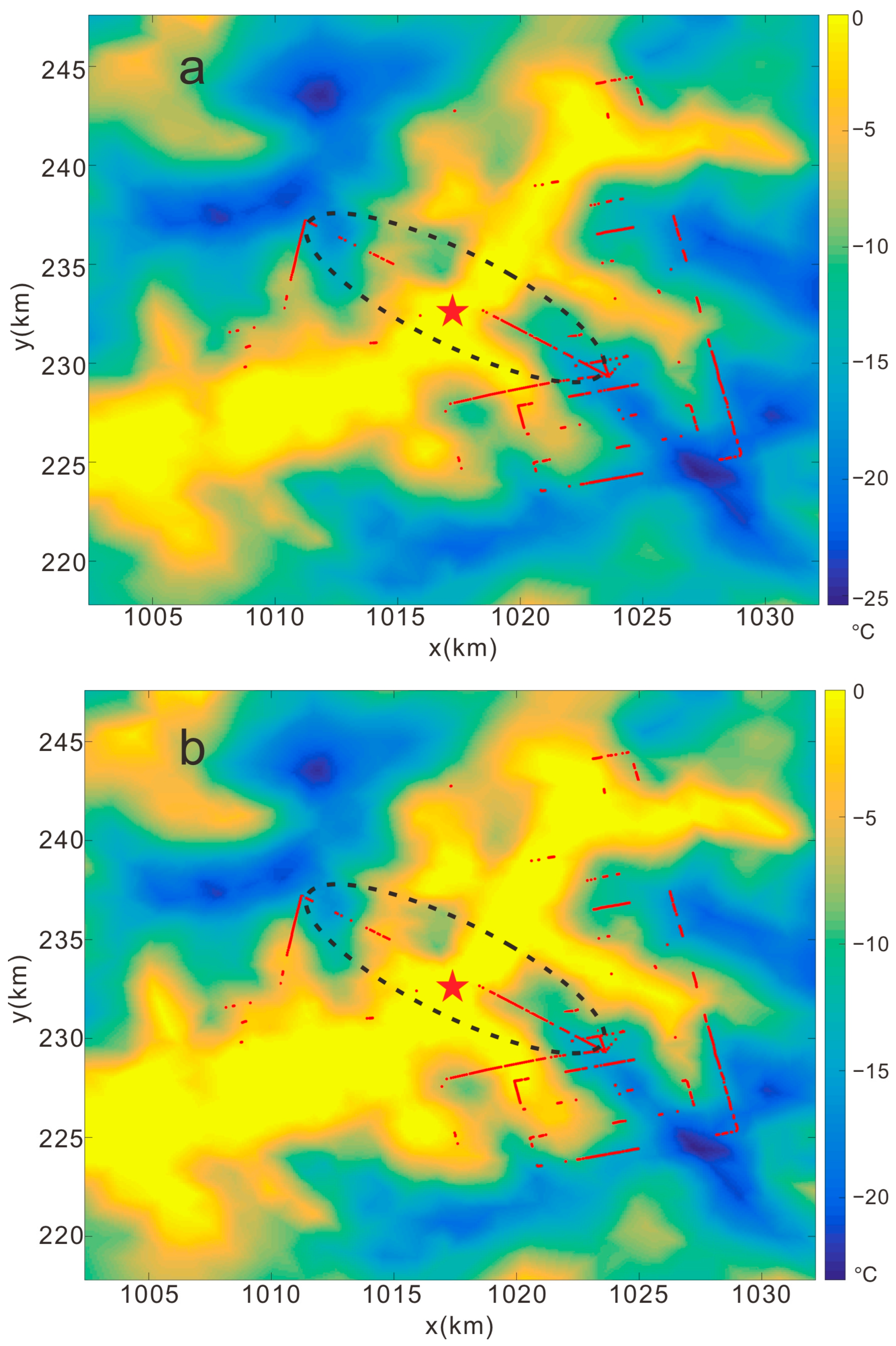
4.1. Various Depth-Averaged Attenuation Rates

In Equation (6), depth-averaged attenuation rates N ¯ can be obtained from L i /z plots (Figure 3). This process simplified the influence of all englacial depth reflectors and the reflection changes. The depth-averaged attenuation rates are often obtained by ordinary least squares [18,42,43] and weighted least squares methods [30]. This method represents the depth-averaged attenuation of all reflectors in the study area rather than every single reflector. However, the attenuation rate depends on the englacial chemistry, the temperature of the ice column, ice thickness and thermal boundary conditions [30]. Additionally, the depth-averaged attenuation rate is often used as an empirical measurement, representing the one-dimensional dependence of attenuation rate on ice thickness without considering the nonlinear dependence on other conditions.
In previous studies, the depth-averaged attenuation rates N ¯ were assumed to be stable along parts of the radar profile. These attenuation rates can be estimated according to the plots of the loss term L i and ice thickness [18,19,24,43]. In Figure 3a–e, plots of L i evaluated from Equation (5) based on the surface and bedrock reflectivity of the radar data during CHINARE 21 in the Dome A region at different depths are shown (red points). The reflectivity-coefficient variation in bedrock leads to the scattering of L i points from the same depth of bedrock, which indicates the difference in bedrock characterization [18].
In Figure 3, the slope of the orange lines are the depth-averaged attenuation rates obtained from the radar data analysis of CHINARE 21 in the Dome A region. As is clear from figures, the depth-averaged attenuation rates show a significant fluctuation in four triangles radar profiles ( N ¯ = 15 dB/km, 5.7 dB/km, 8.4 dB/km, and 11 dB/km from Figure 3a–d), with N ¯ = 9.7 dB/km of all radar data plotted. We selected depth-averaged attenuation rates of 9.7 ± 1.3 dB/km based on the sudden changes in the R values plots (see in the next section) to determine the maximal range of wet bedrock interfaces around the drilling site at Kunlun Station.
Figure 4 shows the plot of L i and ice thickness of the CHINARE 29. Compared with CHINARE 21, the radar profiles of CHINARE 29 are distributed in a narrow zone, and the ice absorption obtained from CHINARE 29 radar data shows a fine linear trend. A depth-averaged attenuation rate of N ¯ = 28 dB/km can be obtained by fitting these absorption losses.

4.2. Analysis of the Reflectivity Variation ( Δ R )

In Figure 3 and Figure 4, the scattering of the absorption loss points with the same depth is due to the reflectivity coefficient of the ice–bedrock interface ( Δ R ≠ 0). The plots of loss term L i obtained from the radar data show linear trends (Figure 3e and Figure 4), representing the depth-averaged attenuation rate N ¯ described previously [18]. Additionally, N ¯ is not constant over wide zones, as the ice temperature and chemical properties change in the ice column [18,31,32]. It is clear from Figure 3e and Figure 4 that the absorption loss points of the CHINARE 21 radar data around the drilling site are more scattered than CHINARE 29, indicating a higher proportion of wet points and making the depth-averaged attenuation rates challenging to obtain accurately. Therefore, we selected the values between the attenuation rates N ¯ obtained from all radar data plots and the plots of four triangle radar profiles of CHINARE 21. We also attempted various depth-averaged attenuation rates in previous studies, including those based on Wolovick et al. and MacGregor et al. [10,44]. In the attempt process, we checked the results of melting point selection, including the minimum ( N ¯ = 5.8 dB/km) and maximum depth average attenuation rate ( N ¯ = 15 dB/km), to eliminate the influence of ion concentration, ice temperature, and other factors on attenuation rate. MacGregor et al. indicated that the attenuation rates shift caused by these factors can reach 10 dB [21,28,44,45]. The N ¯ = 9.7 ± 1.3 dB/km attenuation rates show preferable results in the reflectivity variation ( Δ R ) plots (Figure 5). Additionally, the CHINARE 29 radar data analysis uses N ¯ = 28 dB/km as the attenuation rate.
Figure 5 shows the reflectivity variation ( Δ R ) plots around the drilling site at Kunlun Station in the Dome A region using CHINARE 21 radar data (four triangles). In the plotting process, we used Equation (5) to calculate the loss term L i in the glacier based on the surface and basal reflectivity. Additionally, the loss term L i is calculated from the average depth attenuation rate N ¯ and ice thickness (multiplying the N ¯ by twice the depth). Additionally, the reflectivity variation Δ R can be calculated by Equation (7). The plots of Δ R will help to distinguish the wet or dry ice–bedrock interfaces. In Figure 5, the Δ R points in the orange dashed line zones show the areas with sudden changes in the reflectivity plot ( Δ R > 7.7 dB, the threshold indicated by the red line in the figure), indicating the existence of a wet interface (melting points). To attempt various depth-averaged attenuation rates, we assume all these areas with sudden changes to be the melting points. Additionally, we adjusted the average attenuation rate N ¯ to ensure all these sudden reflectivity changes were over the threshold. As a result, we allowed some false positives as melting points, and obtained the depth-averaged attenuation rate N ¯ = 9.7 ± 1.3 dB/km of the CHINARE 21 radar data.

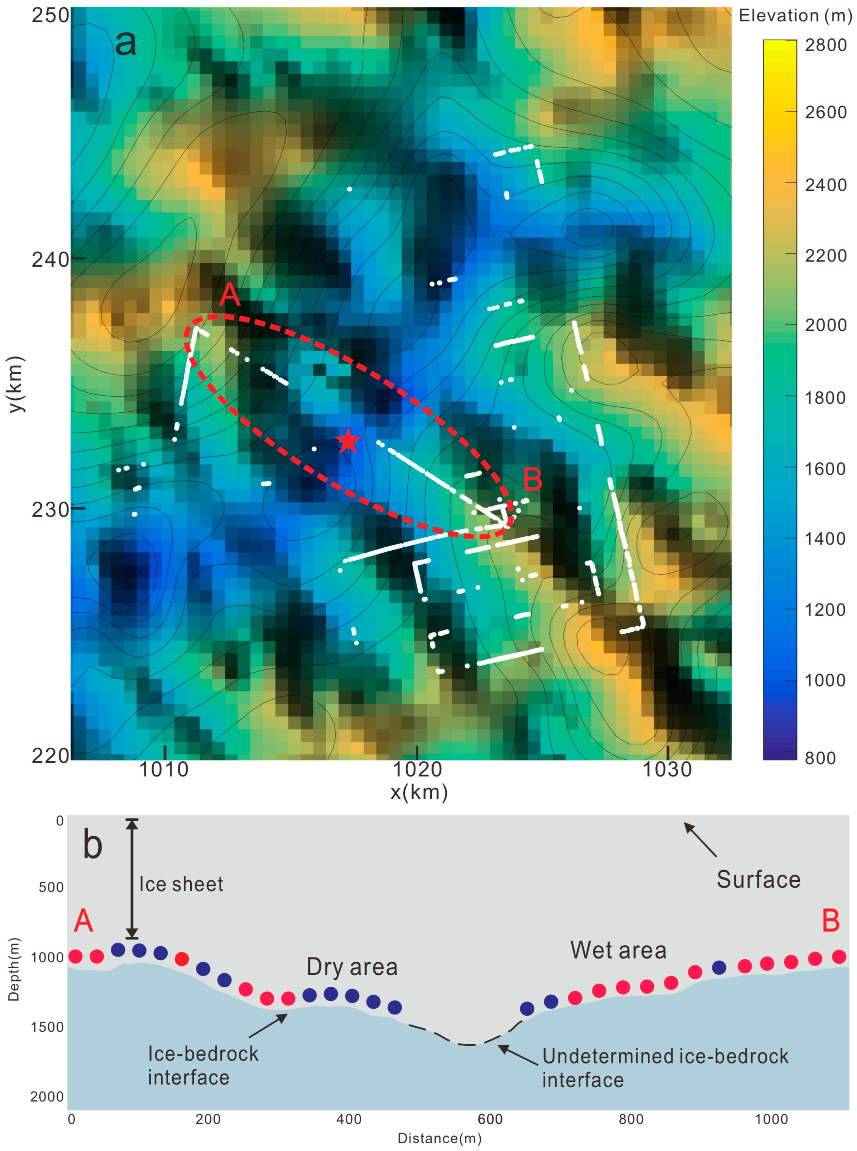
4.3. Wet Bed Condition Map on Bedrock Elevation

According to the above analysis, we plotted the bed conditions with a reflectivity change value higher than the threshold along the radar profiles. These points on a bedrock elevation map reveal the distribution patterns of wet areas around the drilling site at Kunlun Station (Figure 6a). Based on the CHINARE 21 radar data, we also plotted a dry–wet schematic diagram along a radar profile cross-section of the valley bottom. Figure 6 will reveal the impact of basal topography on the wet points. In Figure 6b, the dry areas are mainly concentrated at local high places and above the undetermined ice-bedrock interface area, which may be related to the conduction dominated frozen-on ice [12]. Additionally, the wet areas are mainly concentrated on steep slopes, which may be linked to the direction of water flow [46].

5. Discussion

In CHINARE 21 and 29, the radar data collected in the Dome A region were used to identify the internal isochrone [9,37,38]. These data are reliable for plotting the wet or dry ice–bedrock interface map in this research. Based on the results of the determining and plotting, Figure 6a shows the distribution of wet ice–bedrock interfaces around the drilling site at Kunlun Station. It is clear from the figure that: (1) wet bed conditions determined by two radar systems are locally continuous and scatter in both the northeast and southwest of the Kunlun drilling site; (2) these wet points are mainly present on the northeast valley wall, which may be the consequence of the basal topography and hydraulic potential [12,19]; (3) most of the continuous wet points are distributed along the direction of the slope; and (4) few wet points exist in the east of the drilling site. As identifying the ice–bedrock interface is challenging in the valley bottom area, it is hard to determine wet or dry bed conditions in the valley bottom. Figure 6b illustrates the distribution of wet and dry points along the radar profile across the valley bottom, which may help us to discuss the basal melt near the Kunlun drilling site. In Figure 6b, wet points on the southwest side of the drilling site are lesser than on the northeast side, similar to the overall trend shown in Figure 6a. This phenomenon may be due to the difference in bedrock topography and the hydraulic potential on both sides of the valley. Additionally, dry points are scattered on both sides of the valley above the undetermined ice–bedrock interface area.
Figure 7 shows the plot of wet points on the model basal temperature map using a geothermal heat flux of 55 mW m−2 (a) and 60 mW m−2 (b) [11]. The undetermined ice–bedrock interface mainly exists in the high basal temperature area, so only a few wet points are scattered in the area above −5 °C. Most wet points are located in areas with −10 °C basal temperature, and a few melting points are scattered in lower-temperature areas. Based on the analysis of Figure 6 and Figure 7, the melting trend identified around the drilling site at Kunlun Station in the Dome A region is relatively clear. In the study area, wet points are primarily present in the direction of decreasing hydraulic potential, which is controlled by basal topography and hydraulic gradient [12]. The surface slope around the drilling site is very low, so the water potential mainly depends on the bedrock elevation. Thus, the wet points are primarily concentrated northeast of Kunlun Station and gradually increase with the bedrock elevation. Additionally, most wet points are mainly scattered on the valley wall with low temperatures. This character is similar to the melting and freeze-on in the Dome A region proposed by Bell et al. [12]. The marked radar profile in Figure 6a and Figure 7 shows the potential melting trend controlled by the topography and temperatures. Especially in the southwest part of the marked radar profile, wet points mainly exist in the gentle slope areas with higher temperatures (about −10 °C) and frozen at low-temperature slopes. These wet trends may protect the GSM from glacier erosion [47].
The Dome A region satisfies the potential old-ice drilling sites requirement, with the slow ice flow, thick ice, cold basal conditions, and low accumulation rate [1,3,4,5,6,7,11]. However, the widespread persistent thickening by freezing from the bed in Dome A made it challenging to ensure the existence of the oldest ice [11,12]. Figure 6a and Figure 7 also show the widespread wet points around the drilling site at Kunlun Station. The wet points determined by the CHINARE 21 radar data account for 11.8% of the total. Wet points determined by the CHINARE 29 radar data only account for 3.62%. These melting trends indicate that wet points are scattered along the valley wall in the direction of the water flow, which may lead to potential melting at the valley bottom. However, the process of basal freeze-on is still undetermined [11,12]. Additionally, dry points were determined above both sides of the undetermined ice–bedrock interface area (Figure 6b). Such results are consistent with the previous assumption that the freeze-on process may raise the basal ice by accretion and move the old ice to a higher altitude of the ice sheet [11,12]. This assumption may increase the potential that there is preserved ancient ice around the drilling site at Kunlun Station. Previous studies summarize that reasonably old ice may preserve tens to hundreds of meters above the bed, and the expected 1-million-year-old ice may be located at least 200 m above the ice bed [11]. Conversely, the valley bottom with a higher basal temperature will promote the melting process before freeze-on, which may destroy the old ice with ancient climate records [11,12].

6. Conclusions

We evaluated the wet points around the DK-1 drilling site at Kunlun Station in the Dome A region based on the continuous radar profiles of different IPR systems (CHINARE 21 and CHINARE 29 radar data). The linear absorption model, artificial intelligence model, and various depth-averaged attenuation rates were used during the determination and plotting process. The wet maps on the bedrock elevation and the modal basal temperature show that basal topography is the primary factor controlling the distribution of wet points, and basal temperature influences the basal melt at the flat terrain area. The melting trends show that dry points are scattered above both sides of the undetermined ice–bedrock interface area, similar to the frozen-on phenomenon in the Dome A region. These frozen-on points may induce the movement of old ice to a higher elevation beneath the ice sheet and make it possible to find older ice from hundreds of meters above the base. Additionally, the impact of these wet and dry points on ice core drilling still requires more detailed research on the frozen-on process in the Dome A region.

Author Contributions

Conceptualization, X.T.; methodology, H.W., K.L. and S.D.; software, K.L. and S.D.; validation, H.W.; data curation, K.L. and B.S.; writing—original draft preparation, H.W.; writing—review and editing, X.T.; supervision, X.T. and E.X. All authors have read and agreed to the published version of the manuscript.

Funding

This study was supported by the National Key Research and Development Program of China (Nos. 2019YFC1509102, 2021YFB3900105-7) and the National Natural Science Foundation of China (Nos. 42276257, 41876230, 41941006).

Acknowledgments

The authors thank the Chinese National Antarctic Research Expedition for their help in the field data collection.

Conflicts of Interest

The authors declare no conflict of interest.

References

  1. Sun, B.; Moore, J.C.; Zwinger, T.; Zhao, L.; Steinhage, D.; Tang, X.; Zhang, D.; Cui, X.; Martín, C. How old is the ice beneath Dome A, Antarctica? Cryosphere 2014, 8, 1121–1128. [Google Scholar] [CrossRef] [Green Version]
  2. Zhang, N.; An, C.; Fan, X.; Shi, G.; Li, C.; Liu, J.; Hu, Z.; Talalay, P.; Sun, Y.; Li, Y. Chinese First Deep Ice-Core Drilling Project DK-1 at Dome A, Antarctica (2011–2013): Progress and performance. Ann. Glaciol. 2014, 55, 88–98. [Google Scholar] [CrossRef] [Green Version]
  3. Hu, Z.; Shi, G.; Talalay, P.; Li, Y.; Fan, X.; An, C.; Zhang, N.; Li, C.; Liu, K.; Yu, J.; et al. Deep ice-core drilling to 800 m at Dome A in East Antarctica. Ann. Glaciol. 2021, 62, 293–304. [Google Scholar] [CrossRef]
  4. Sun, B.; Siegert, M.J.; Mudd, S.M.; Sugden, D.; Fujita, S.; Cui, X.; Jiang, Y.; Tang, X.; Li, Y. The Gamburtsev mountains and the origin and early evolution of the Antarctic ice sheet. Nature 2009, 459, 690–693. [Google Scholar]
  5. Hou, S.; Li, Y.; Xiao, C.; Ren, J. Recent accumulation rate at Dome A, Antarctic. Chin. Sci. Bull. 2007, 52, 428–431. [Google Scholar] [CrossRef]
  6. Yang, Y.; Sun, B.; Wang, Z.; Ding, M.; Hwang, C.; Ai, S.; Wang, L.; Du, Y.; Dongchen, E. GPS-derived velocity and strain fields around Dome Argus, Antarctica. J. Glaciol. 2014, 60, 735–742. [Google Scholar] [CrossRef] [Green Version]
  7. Jiang, S.; Cole-Dai, J.; Li, Y.; Ferris, D.G.; Ma, H.; An, C.; Shi, G.; Sun, B. A detailed 2840 year record of explosive volcanism in a shallow ice core from Dome A, East Antarctica. J. Glaciol. 2012, 58, 65–75. [Google Scholar] [CrossRef] [Green Version]
  8. Tang, X.; Sun, B.; Wang, T. Radar isochronic layer dating for a deep ice core at Kunlun Station, Antarctica. Sci. China Earth Sci. 2020, 63, 139–144. [Google Scholar] [CrossRef]
  9. Tang, X.; Sun, B.; Zhang, Z.; Zhang, X.; Cui, X.; Li, X. Structure of the internal isochronous layers at Dome A, East Antarctica. Sci. China Earth Sci. 2011, 54, 445–450. [Google Scholar] [CrossRef]
  10. Wolovick, M.J.; Robin, E.B.; Timothy, T.C.; Frearson, N. Identification and control of subglacial water networks under Dome A, Antarctica. J. Geophys. Res. Earth Surf. 2013, 118, 140–154. [Google Scholar] [CrossRef]
  11. Zhao, L.; Moore, J.C.; Sun, B.; Tang, X.; Guo, X. Where is the 1-million-year-old ice at Dome A? Cryosphere 2018, 12, 1651–1663. [Google Scholar] [CrossRef] [Green Version]
  12. Bell, R.E.; Ferraccioli, F.; Creyts, T.T.; Braaten, D.; Corr, H.; Das, I.; Damaske, D.; Frearson, N.; Jordan, T.; Rose, K.; et al. Widespread Persistent Thickening of the East Antarctic Ice Sheet by Freezing from the Base. Science 2011, 331, 1592–1595. [Google Scholar] [CrossRef]
  13. Wrona, T.; Wolovick, M.J.; Ferraccioli, F.; Corr, H.; Jordan, T.A.; Siegert, M. Position and variability of complex structures in the central East Antarctic Ice Sheet. Geol. Soc. Lond. Spec. Publ. 2018, 461, 113. [Google Scholar] [CrossRef] [Green Version]
  14. Bentley, C.R.; Lord, N.; Liu, C. Radar reflections reveal a wet bed beneath stagnant Ice Stream C and a frozen bed beneath ridge BC, West Antarctica. J. Glaciol. 1998, 44, 149–156. [Google Scholar] [CrossRef] [Green Version]
  15. Bindschadler, R. Monitoring ice sheet behavior from space. Rev. Geophys. 1998, 36, 79–104. [Google Scholar] [CrossRef] [Green Version]
  16. Catania, G.A.; Conway, H.B.; Gades, A.M.; Raymond, C.F.; Engelhardt, H. Bed reflectivity beneath inactive ice streams in West Antarctica. Ann. Glaciol. 2003, 36, 287–291. [Google Scholar] [CrossRef] [Green Version]
  17. Peters, M.E.; Blankenship, D.D.; Morse, D.L. Analysis techniques for coherent airborne radar sounding: Application to West Antarctic ice streams. J. Geophys. Res. 2005, 110, B06303. [Google Scholar] [CrossRef]
  18. Zirizzotti, A.; Cafarella, L.; Baskaradas, J.A.; Tabacco, I.E.; Urbini, S.; Mangialetti, M.; Bianchi, C. Dry–Wet Bedrock Interface Detection by Radio Echo Sounding Measurements. IEEE Trans. Geosci. Remote Sens. 2010, 48, 2343–2348. [Google Scholar] [CrossRef]
  19. Lindzey, L.E.; Beem, L.H.; Young, D.A.; Quartini, E.; Blankenship, D.D.; Lee, C.K.; Lee, W.; Lee, J.; Lee, J. Aerogeophysical characterization of an active subglacial lake system in the David Glacier catchment, Antarctica. Cryosphere 2020, 14, 2217–2233. [Google Scholar] [CrossRef]
  20. Yan, S.; Blankenship, D.D.; Greenbaum, J.; Young, D.; Li, L.; Rutishauser, A.; Guo, J.; Roberts, J.L.; van Ommen, T.D.; Siegert, M.; et al. A newly discovered subglacial lake in East Antarctica likely hosts a valuable sedimentary record of ice and climate change. Geology 2022, 50, 949–953. [Google Scholar] [CrossRef]
  21. Macgregor, J.A.; Matsuoka, K.; Studinger, M. Radar detection of accreted ice over Lake Vostok, Antarctica. Earth Planet. Sci. Lett. 2009, 282, 222–233. [Google Scholar] [CrossRef]
  22. Dowdeswell, J.A.; Siegert, M. The physiography of modern Antarctic subglacial lakes. Global Planet. Chang. 2003, 35, 221–236. [Google Scholar] [CrossRef]
  23. Carter, S.P. Radar-based subglacial lake classification in Antarctica, Geochem. Geophys. Geosy. 2007, 8, Q03016. [Google Scholar] [CrossRef]
  24. Zirizzotti, A.; Cafarella, L.; Urbini, S. Ice and Bedrock Characteristics Underneath Dome C (Antarctica) From Radio Echo Sounding Data Analysis. IEEE Trans. Geosci. Remote Sens. 2012, 50, 37–43. [Google Scholar] [CrossRef]
  25. Urbini, S.; Cafarella, L.; Tabacco, I.E.; Baskaradas, J.A.; Serafini, M.; Zirizzotti, A. RES Signatures of Ice Bottom Near to Dome C (Antarctica). IEEE Trans. Geosci. Remote Sens. 2014, 53, 1558–1564. [Google Scholar] [CrossRef]
  26. Hills, B.H.; Christianson, K.; Holschuh, N. A framework for attenuation method selection evaluated with ice-penetrating radar data at South Pole Lake. Ann. Glaciol. 2020, 61, 176–187. [Google Scholar] [CrossRef]
  27. Fujita, S.; Holmlund, P.; Matsuoka, K.; Enomoto, H.; Fukui, K.; Nakazawa, F.; Sugiyama, S.; Surdyk, S. Radar diagnosis of the subglacial conditions in Dronning Maud Land, East Antarctica. Cryosphere 2012, 6, 1203–1219. [Google Scholar] [CrossRef] [Green Version]
  28. Macgregor, J.A.; Winebrenner, D.P.; Conway, H.; Matsuoka, K.; Mayewski, P.A.; Clow, G.D. Modeling Englacial Radar Attenuation at Siple Dome, West Antarctica, Using Ice Chemistry and Temperature Data. J. Geophys. Res.-Atmos. 2007, 112, F03008. [Google Scholar] [CrossRef] [Green Version]
  29. Jordan, T.M.; Bamber, J.L.; Williams, C.N.; Paden, J.; Siegert, M.; Huybrechts, P.; Gagliardini, O.; Gillet-Chaulet, F. An ice-sheet-wide framework for englacial attenuation from ice-penetrating radar data. Cryosphere 2016, 10, 1547–1570. [Google Scholar] [CrossRef] [Green Version]
  30. Macgregor, J.A.; Li, J.; Paden, J.; Catania, G.; Clow, G.D.; Fahnestock, M.; Gogineni, S.P.; Grimm, R.; Morlighem, M.; Nandi, S.; et al. Radar attenuation and temperature within the Greenland Ice Sheet. J.Geophys. Res. Earth Surf. 2015, 120, 983–1008. [Google Scholar] [CrossRef] [Green Version]
  31. Matsuoka, K.; Morse, D.; Raymond, C.F. Estimating englacial radar attenuation using depth profiles of the returned power, central West Antarctica. J. Geophys. Res. Earth Surf. 2010, 115, 1–15. [Google Scholar] [CrossRef] [Green Version]
  32. Matsuoka, K.; Macgregor, J.A.; Pattyn, F. Predicting radar attenuation within the Antarctic ice sheet. Earth Planet. Sci. Lett. 2012, 359–360, 173–183. [Google Scholar] [CrossRef]
  33. Matsuoka, K.; Pattyn, F.; Callens, D.; Conway, H. Radar characterization of the basal interface across the grounding zone of an ice-rise promontory in East Antarctica. Ann. Glaciol. 2012, 53, 29–34. [Google Scholar] [CrossRef] [Green Version]
  34. Holschuh, N.; Christianson, K.; Anandakrishnan, S.; Alley, R.B.; Jacobel, R.W. Constraining attenuation uncertainty in common midpoint radar surveys of ice sheets. J.Geophys. Res. Earth Surf. 2016, 121, 1876–1890. [Google Scholar] [CrossRef] [Green Version]
  35. Bingham, R.G.; Siegert, M.J. Radio-Echo Sounding Over Polar Ice Masses. J. Environ. Eng. Geoph. 2007, 12, 47–62. [Google Scholar] [CrossRef] [Green Version]
  36. Cui, X.; Sun, B.; Tian, G.; Tang, X.; Zhang, X.; Jiang, Y.; Guo, J.; Li, X. Ice radar investigation at Dome A, East Antarctica: Ice thickness and subglacial topography. Chin. Sci. Bull. 2010, 55, 425–431. [Google Scholar] [CrossRef]
  37. Tang, X.; Sun, B.; Guo, J.; Cui, X.; Zhao, B.; Chen, Y. A freeze-on ice zone along the Zhongshan–Kunlun ice sheet profile, East Antarctica, by a new ground-based ice-penetrating radar. Sci. Bull. 2015, 60, 574–576. [Google Scholar] [CrossRef] [Green Version]
  38. Tang, X.; Sun, B.; Wang, T. Internal layering structure and subglacial conditions along a traverse line from Zhongshan Station to Dome A, East Antarctica, revealed by ground-based radar sounding. Appl. Geophys. 2020, 17, 870–878. [Google Scholar] [CrossRef]
  39. Cui, X.; Wang, T.; Sun, B.; Tang, X.; Guo, J. Chinese radioglaciological studies on the Antarctic ice sheet: Progress and prospects. Adv. Polar Sci. 2017, 28, 14–23. [Google Scholar]
  40. Dong, S.; Tang, X.; Guo, J.; Fu, L.; Chen, X.; Sun, B. EisNet: Extracting Bedrock and Internal Layers From Radiostratigraphy of Ice Sheets With Machine Learning. IEEE Trans. Geosci. Remote Sens. 2022, 60, 1–12. [Google Scholar] [CrossRef]
  41. Tang, X.; Luo, K.; Dong, S.; Zhang, Z.; Sun, B. Quantifying Basal Roughness and Internal Layer Continuity Index of Ice Sheets by an Integrated Means with Radar Data and Deep Learning. Remote Sens. 2022, 14, 4507. [Google Scholar] [CrossRef]
  42. Jacobel, R.W.; Welch, B.C.; Osterhouse, D.; Pettersson, R.; Gregor, J.A.M. Spatial variation of radar-derived basal conditions on Kamb Ice Stream, West Antarctica. Ann. Glaciol. 2009, 50, 10–16. [Google Scholar] [CrossRef] [Green Version]
  43. Winebrenner, D.; Smith, B.; Catania, G.; Conway, H.; Raymond, C. Radio frequency attenuation beneath Siple dome, West antarctica, from wide angle and profiling radar observations. Ann. Glaciol. 2003, 37, 226–232. [Google Scholar] [CrossRef] [Green Version]
  44. MacGregor, J.A.; Matsuoka, K.; Waddington, E.D.; Winebrenner, D.P.; Pattyn, F. Spatial variation of englacial radar attenuation: Modeling approach and application to the Vostok flowline. J.Geophys. Res. Earth Surf. 2012, 117, 1–15. [Google Scholar] [CrossRef] [Green Version]
  45. MacGregor, J.A.; Anandakrishnan, S.; Catania, G.A.; Winebrenner, D.P. The grounding zone of the Ross Ice Shelf, West Antarctica, from ice-penetrating radar. J. Glaciol. 2011, 57, 917–928. [Google Scholar] [CrossRef] [Green Version]
  46. Olivier, P.; Catherine, R.; Frédéric, P.; Stefano, U.; Massimo, F. Geothermal flux and basal melt rate in the Dome C region inferred from radar reflectivity and heat modelling. Cryosphere 2017, 11, 2231–2246. [Google Scholar]
  47. Paxman, G.J.G.; Watts, A.B.; Ferraccioli, F.; Jordan, T.A.; Bell, R.E.; Jamieson, S.S.R.; Finn, C.A. Erosion-driven uplift in the Gamburtsev Subglacial Mountains of East Antarctica. Earth Planet. Sci. Lett. 2016, 452, 1–14. [Google Scholar] [CrossRef] [Green Version]
Figure 1. Bedrock topography in the vicinity of Dome A and Kunlun Station (contour spacing 100 m), white lines show ground-based radar surveys, asterisks show the Kunlun Station and the Dome A, 1–4 show the radar paths during the CHINARE 21, 5–8 show the radar paths during the CHINARE 29.
Remotesensing 15 01726 g001
Figure 2. (ad). Radar profiles of CHINARE 29; white lines show the ice–bedrock interfaces extracted by EisNet; (e) the positions of extracted results around the drilling site at Kunlun Station in the Dome A region (white arrows represent the direction of the radar path).
Remotesensing 15 01726 g002
Figure 3. Absorption loss (red points) radar data of the CHINARE 21 compared with linear trends (orange lines) with slopes of about 15 dB/km, 5.7 dB/km, 8.4 dB/km, 11 dB/km, and 9.7 dB/km (ad): absorption loss radar data of four triangles of CHINARE 21 in Dome A region, (e): all radar data of CHINARE 21 in Dome A region).
Remotesensing 15 01726 g003
Figure 4. Absorption loss (red points) radar data of the CHINARE 29 compared with linear trends (orange line) with slopes of about N ¯ = 28 dB/km.
Remotesensing 15 01726 g004
Figure 5. Reflectivity variation plots along four radar profiles calculated using a linear absorption model and the CHINARE 21 radar data; the vertical lines show Δ R > 7.7 dB area (radar data at the undetermined ice-bedrock interfaces area were removed).
Remotesensing 15 01726 g005
Figure 6. (a). Wet map on a color bedrock elevation map (contour spacing 100 m) around drilling site at Kunlun Station in the Dome A region; white points are wet points, asterisk is the Kunlun Station. (b). Dry–wet schematic diagram of the marked area in (a) (red points for wet ice–bedrock interface s; blue points for dry ice–bedrock interfaces).
Remotesensing 15 01726 g006
Figure 7. Wet (red) bed conditions on the modeled basal temperature map using geothermal heat flux of 55 mW m−2 (a) and 60 mW m−2 (b) (the red asterisk is Kunlun Station drilling site). The base map is from Zhao et al., 2018 [11].
Remotesensing 15 01726 g007
Table 1. Technical characteristics of IPR systems used during CHINARE 21 and CHINARE 29 [39].
Radar SystemsCHINARE 21
Dual-Frequency Radar
CHINARE 29
Developed Deep IPR
AntennaThree-element YagiLog-periodical
Center frequency/MHz60/179150
Peak power/kW10.5
Pulse width/μs250/500/10002000/4000/8000
Sampling time window/μs5050
Sampling frequency/MHz100500
Noise/dB<1<3
Dynamic range/dB80>110
Bandwidth/MHz4100
Antenna gain/dBi7.29
Beam width/(°)7060
Table 2. Power loss of interface [18].
Interface (Reflection/Transmission Losses)Power Loss L (dB)
ice–air ( T a i )0.35
air–ice ( R a i )11.0
ice–water ( R i w )3.5
ice–rock ( R i r )11.2
Disclaimer/Publisher’s Note: The statements, opinions and data contained in all publications are solely those of the individual author(s) and contributor(s) and not of MDPI and/or the editor(s). MDPI and/or the editor(s) disclaim responsibility for any injury to people or property resulting from any ideas, methods, instructions or products referred to in the content.

