
Inversion of Upstream Solar Wind Parameters from ENA Observations at Mars
 , , and
Abstract
: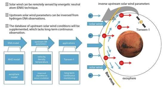
1. Introduction
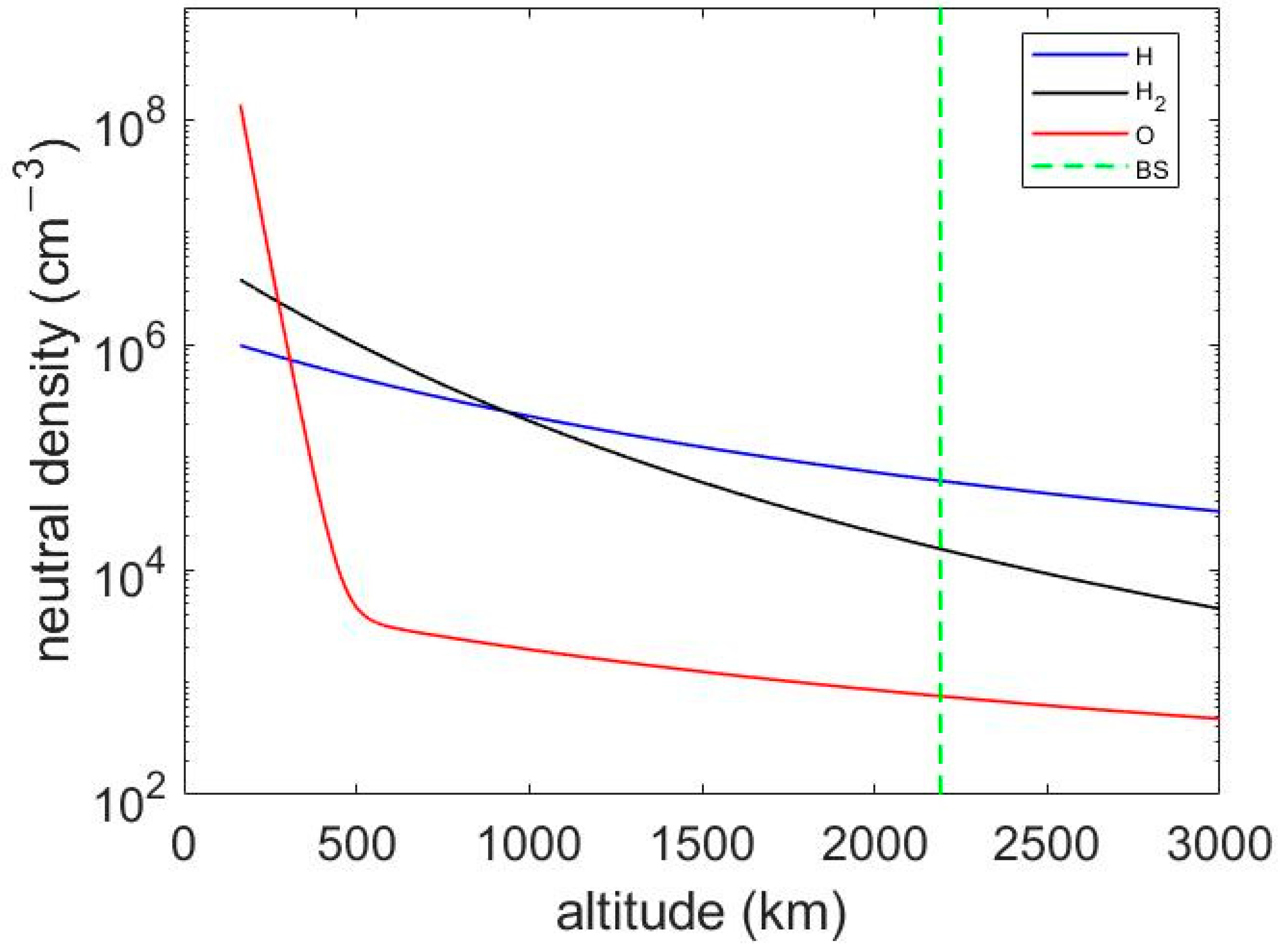
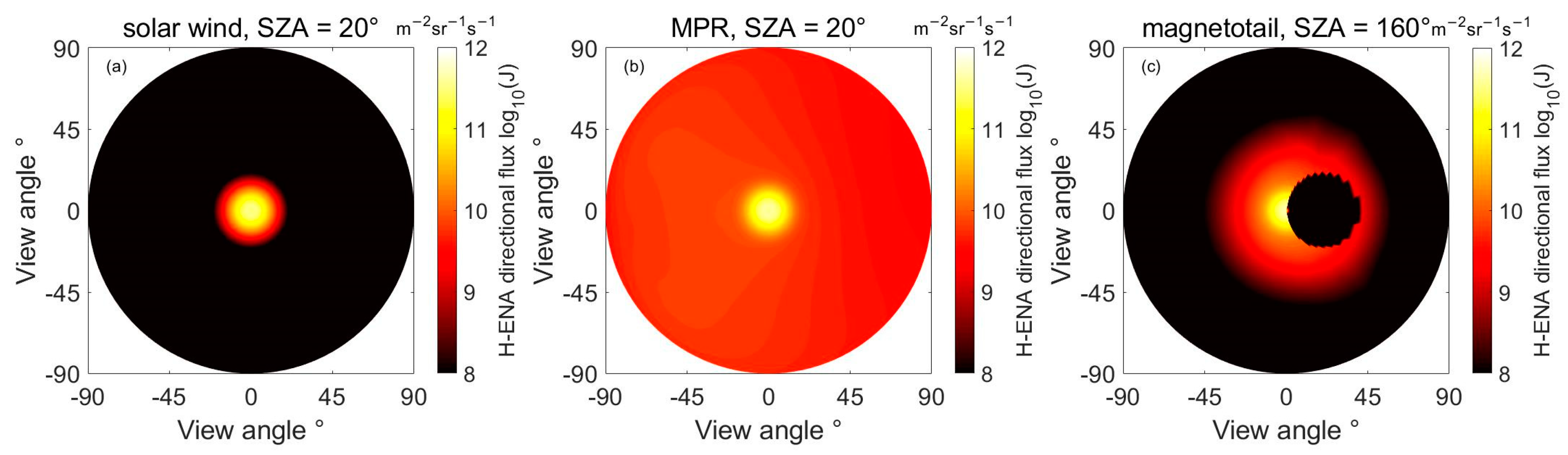
2. Modeling H-ENA
- H+ + H → H + H+;
- H+ + O → H + O+;
- H+ + H2 → H + H2+.
3. Inversion of Solar Wind Parameters from H-ENA Observation
3.1. Basic Algorithm
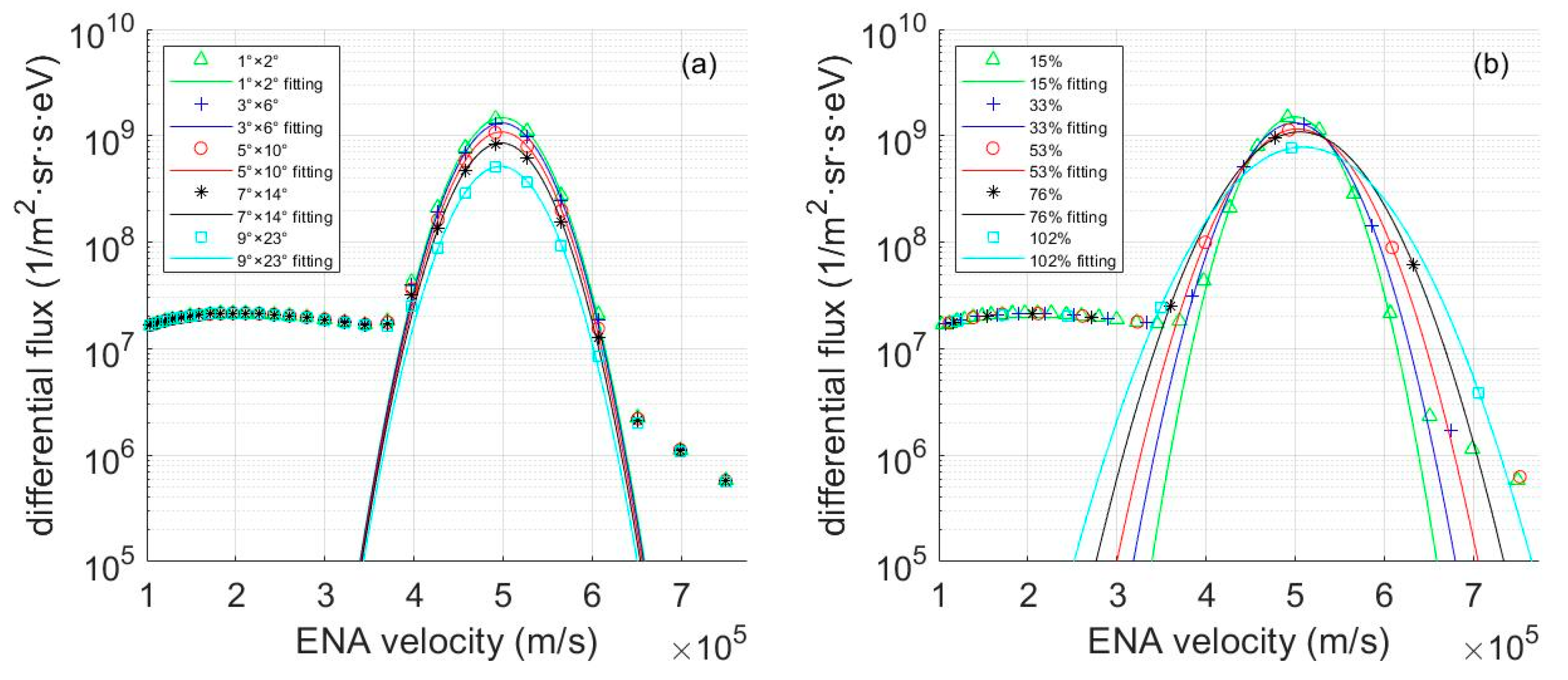
3.2. Resolution in Inversion
3.3. Mitigating the Angular Resolution Effect
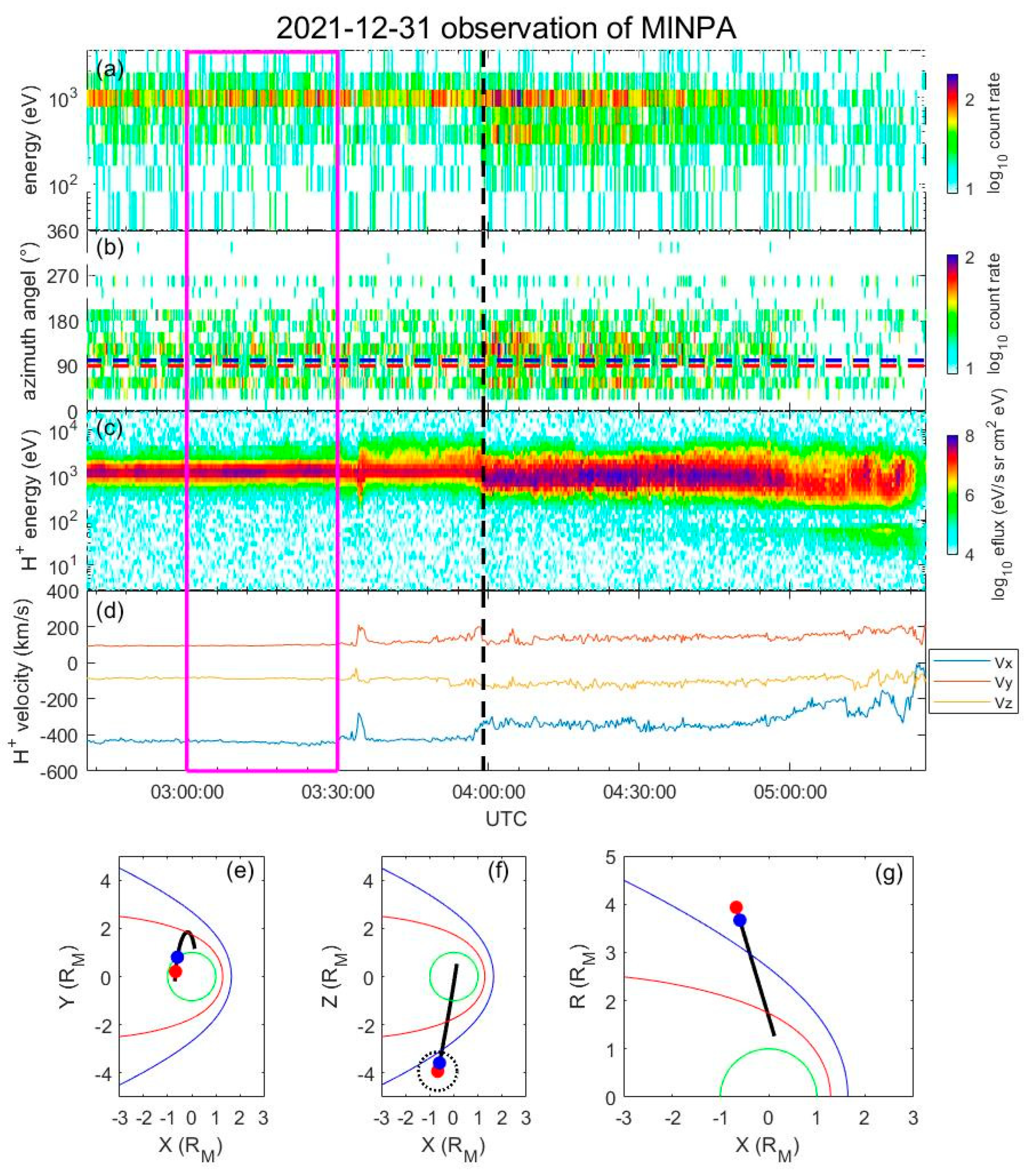
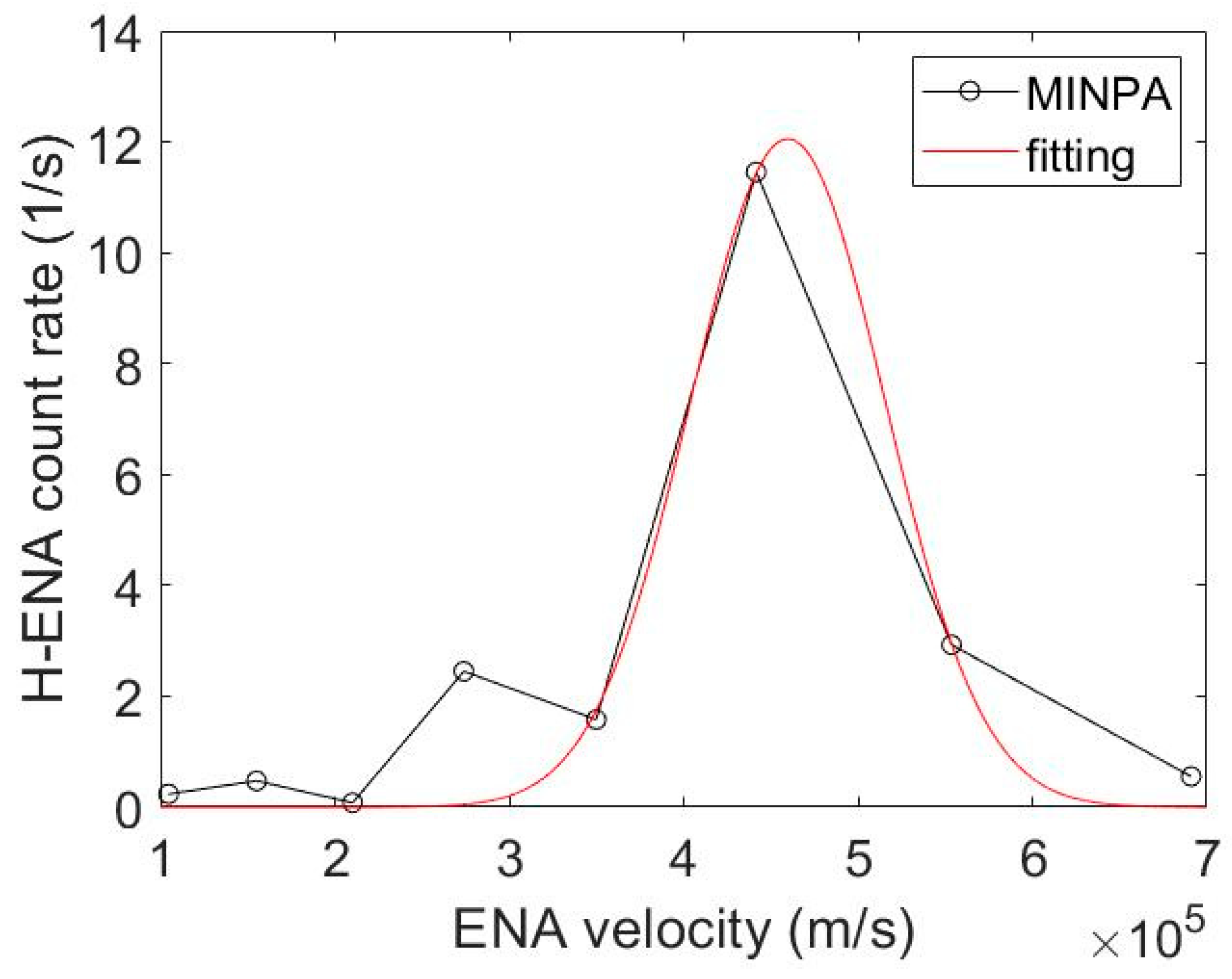
3.4. Application to Tianwen-1 Observation
4. Discussion
5. Conclusions
Author Contributions
Funding
Data Availability Statement
Acknowledgments
Conflicts of Interest
References
- Swaczyna, P.; McComas, D.J.; Zirnstein, E.J.; Heerikhuisen, J. Angular Scattering in Charge Exchange: Issues and Implications for Secondary Interstellar Hydrogen. Astrophys. J. 2019, 887, 223. [Google Scholar] [CrossRef]
- Gruntman, M. Energetic neutral atom imaging of space plasmas. Rev. Sci. Instrum. 1997, 68, 3617–3656. [Google Scholar] [CrossRef] [Green Version]
- Wurz, P. Detection of Energetic Neutral Atoms. In The Outer Heliosphere: Beyond the Planets; Katlenburg-Lindau: Berlin/Heidelberg, Germany, 2000; pp. 251–288. [Google Scholar]
- Vignes, D.; Mazelle, C.; Rme, H.; Acuna, M.H.; Connerney, J.E.P.; Lin, R.P.; Mitchell, D.L.; Cloutier, P.; Crider, D.H.; Ness, N.F. The Solar Wind interaction with Mars: Locations and shapes of the Bow Shock and the Magnetic Pile-up Boundary from the observations of the MAG/ER experiment onboard Mars Global Surveyor. Geophys. Res. Lett. 2000, 27, 49–52. [Google Scholar] [CrossRef]
- Futaana, Y.; Barabash, S.; Grigoriev, A.; Holmstrom, M.; Kallio, E.; Brandt, P.C.; Gunell, H.; Brinkfeldt, K.; Lundin, R.; Andersson, H.; et al. First ENA observations at Mars: Subsolar ENA jet. Icarus 2006, 182, 413–423. [Google Scholar] [CrossRef]
- Futaana, Y.; Barabash, S.; Grigoriev, A.; Holmstrom, M.; Kallio, E.; Brandt, P.C.; Gunell, H.; Brinkfeldt, K.; Lundin, R.; Andersson, H.; et al. First ENA observations at Mars: ENA emissions from the martian upper atmosphere. Icarus 2006, 182, 424–430. [Google Scholar] [CrossRef]
- Gunell, H.; Brinkfeldt, K.; Holmstrom, M.; Brandt, P.C.; Barabash, S.; Kallio, E.; Ekenback, A.; Futaana, Y.; Lundin, R.; Andersson, H.; et al. First ENA observations at Mars: FCharge exchange ENAs produced in the magnetosheath. Icarus 2006, 182, 431–438. [Google Scholar] [CrossRef]
- Mura, A.; Orsini, S.; Milillo, A.; Kallio, E.; Galli, A.; Barabash, S.; Wurz, P.; Grigoriev, A.; Futaana, Y.; Andersson, H.; et al. ENA detection in the dayside of Mars: ASPERA-3 NPD statistical study. Planet. Space Sci. 2008, 56, 840–845. [Google Scholar] [CrossRef]
- Galli, A.; Wurz, P.; Kallio, E.; Ekenbäck, A.; Holmström, M.; Barabash, S.; Grigoriev, A.; Futaana, Y.; Fok, M.C.; Gunell, H. Tailward flow of energetic neutral atoms observed at Mars. J. Geophys. Res. 2008, 113, E12012. [Google Scholar] [CrossRef]
- Galli, A. Energetic Neutral Atoms Imaging of Mars, Venus, and the Heliosphere; University of Bern: Bern, Switzerland, 2008. [Google Scholar]
- Milillo, A.; Mura, A.; Orsini, S.; Massetti, S.; son Brandt, P.C.; Sotirelis, T.; D’Amicis, R.; Barabash, S.; Frahm, R.A.; Kallio, E.; et al. Statistical analysis of the observations of the MEX/ASPERA-3 NPI in the shadow. Planet. Space Sci. 2009, 57, 1000–1007. [Google Scholar] [CrossRef]
- Ma, J.; Kong, L.; Li, W.; Zhang, Y.; Wurz, P.; Galli, A.; Tang, B.; Xie, L.; Zhang, A.; Li, L. Solar Wind Energetic Neutral Atom Observation at Mars by MINPA Onboard the Tianwen-1 Orbiter. In Proceedings of the Fall Meeting 2022, AGU, Chicago, IL, USA, 12–16 December 2022. [Google Scholar]
- Kallio, E.; Luhmann, J.G.; Barabash, S. Charge exchange near Mars: The solar wind absorption and energetic neutral atom production. J. Geophys. Res. Space Phys. 1997, 102, 22183–22197. [Google Scholar] [CrossRef]
- Wang, X.D.; Alho, M.; Jarvinen, R.; Kallio, E.; Barabash, S.; Futaana, Y. Emission of hydrogen energetic neutral atoms from the Martian subsolar magnetosheath. J. Geophys. Res. Space Phys. 2016, 121, 190–204. [Google Scholar] [CrossRef] [Green Version]
- Wang, X.D.; Alho, M.; Jarvinen, R.; Kallio, E.; Barabash, S.; Futaana, Y. Precipitation of Hydrogen Energetic Neutral Atoms at the Upper Atmosphere of Mars. J. Geophys. Res. Space Phys. 2018, 123, 8730–8748. [Google Scholar] [CrossRef]
- Holmstrom, M.; Barabash, S.; Kallio, E. Energetic neutral atoms at Mars—1. Imaging of solar wind protons. J. Geophys. Res. Space Phys. 2002, 107, 1277. [Google Scholar] [CrossRef]
- Ramstad, R.; Brain, D.A.; Dong, Y.X.; Halekas, J.S.; McFadden, J.P.; Espley, J.; Jakosky, B. Energetic Neutral Atoms near Mars: Predicted Distributions Based on MAVEN Measurements. Astrophys. J. 2022, 927, 11. [Google Scholar] [CrossRef]
- Kallio, E.; Barabash, S.; Brinkfeldt, K.; Gunell, H.; Holmstrom, M.; Futaana, Y.; Schmidt, W.; Sales, T.; Koskinen, H.; Riihela, P.; et al. Energetic Neutral Atoms (ENA) at Mars: Properties of the hydrogen atoms produced upstream of the martian bow shock and implications for ENA sounding technique around non-magnetized planets. Icarus 2006, 182, 448–463. [Google Scholar] [CrossRef]
- Lu, L.; McKenna-Lawlor, S.; Barabash, S.; Brandt, P.C.; Balaz, J.; Liu, Z.X.; He, Z.H.; Reeves, G.D. Comparisons between ion distributions retrieved from ENA images of the ring current and contemporaneous, multipoint ion measurements recorded in situ during the major magnetic storm of 15 May 2005. J. Geophys. Res. Space Phys. 2010, 115, A12218. [Google Scholar] [CrossRef] [Green Version]
- Fuselier, S.A.; Dayeh, M.A.; Galli, A.; Funsten, H.O.; Schwadron, N.A.; Petrinec, S.M.; Trattner, K.J.; McComas, D.J.; Burch, J.L.; Toledo-Redondo, S.; et al. Neutral Atom Imaging of the Solar Wind-Magnetosphere-Exosphere Interaction Near the Subsolar Magnetopause. Geophys. Res. Lett. 2020, 47, e2020GL089362. [Google Scholar] [CrossRef]
- Ma, Y.; Fang, X.; Halekas, J.S.; Xu, S.; Russell, C.T.; Luhmann, J.G.; Nagy, A.F.; Toth, G.; Lee, C.O.; Dong, C.; et al. The Impact and Solar Wind Proxy of the 2017 September ICME Event at Mars. Geophys. Res. Lett. 2018, 45, 7248–7256. [Google Scholar] [CrossRef] [Green Version]
- Gunell, H.; Holmstrom, M.; Barabash, S.; Kallio, E.; Janhunen, P.; Nagy, A.F.; Ma, Y. Planetary ENA imaging: Effects of different interaction models for Mars. Planet. Space Sci. 2006, 54, 117–131. [Google Scholar] [CrossRef]
- Lindsay, B.G.; Stebbings, R.F. Charge transfer cross sections for energetic neutral atom data analysis. J. Geophys. Res. 2005, 110, A12213. [Google Scholar] [CrossRef]
- Rinsuke, I.; Tatsuo, T.; Toshizo, S.; Phaneuf, R.A. Analytic Cross Sections for Collision of H, H2, He and Li Atoms and Ions with Atoms and Melecules; Japan Atomic Energy Research Institute: Ibaraki, Japan, 1993. [Google Scholar]
- Ma, Y.J.; Russell, C.T.; Fang, X.; Dong, Y.; Nagy, A.F.; Toth, G.; Halekas, J.S.; Connerney, J.E.P.; Espley, J.R.; Mahaffy, P.R.; et al. MHD model results of solar wind interaction with Mars and comparison with MAVEN plasma observations. Geophys. Res. Lett. 2015, 42, 9113–9120. [Google Scholar] [CrossRef] [Green Version]
- Ma, Y.J.; Nagy, A.F.; Sokolov, I.V.; Hansen, K.C. Three-dimensional, multispecies, high spatial resolution MHD studies of the solar wind interaction with Mars. J. Geophys. Res. Space Phys. 2004, 109, A07211. [Google Scholar] [CrossRef] [Green Version]
- Chamberlain, J.W.; Hunten, D.M. Theory of Planetary Atmospheres; Academic Press Inc., Ltd.: San Diego, CA, USA, 1987. [Google Scholar]
- Wang, X.D.; Barabash, S.; Futaana, Y.; Grigoriev, A.; Wurz, P. Directionality and variability of energetic neutral hydrogen fluxes observed by Mars Express. J. Geophys. Res. Space Phys. 2013, 118, 7635–7642. [Google Scholar] [CrossRef]
- Kong, L.; Zhang, A.; Tian, Z.; Zheng, X.; Wang, W.; Liu, B.; Wurz, P.; Piazza, D.; Etter, A.; Su, B.; et al. Mars Ion and Neutral Particle Analyzer (MINPA) for Chinese Mars Exploration Mission (Tianwen-1): Design and ground calibration. Earth Planet. Phys. 2020, 4, 333–344. [Google Scholar] [CrossRef]
- Zhang, A.; Kong, L.; Li, W.; Li, L.; Tang, B.; Rong, Z.; Wei, Y.; Ma, J.; Zhang, Y.; Xie, L.; et al. Tianwen-1 MINPA observations in the solar wind. Earth Planet. Phys. 2022, 6, 1–9. [Google Scholar] [CrossRef]
- Anderson, B.J.; Fuselier, S.A. Magnetic pulsations from 0.1 to 4.0 Hz and associated plasma properties in the Earth’s subsolar magnetosheath and plasma depletion layer. J. Geophys. Res. Space Phys. 1993, 98, 1461–1479. [Google Scholar] [CrossRef]
- Jin, T.; Lei, L.; Zhang, Y.; Xie, L.; Qiao, F. Statistical Analysis of the Distribution and Evolution of Mirror Structures in the Martian Magnetosheath. Astrophys. J. 2022, 929, 165. [Google Scholar] [CrossRef]


| Parameter | Value |
|---|---|
| SW density | 1.8 cm−3 |
| SW velocity | (500, 0, 0) km/s |
| SW proton temperature | 1.5 × 10⁵ K |
| SW magnetic field | (−1.6, 2.5, 0) nT |
| Parameter | Temperature | Density |
|---|---|---|
| H | 192 K | 9.9 × 105 cm−3 |
| H2 | 192 K | 3.8 × 106 cm−3 |
| O (thermal) | 173 K | 1.4 × 108 cm−3 |
| O (hot) | 4.4 × 10³ K | 5.5 × 103 cm−3 |
| Angular Resolution | SW Velocity (km/s) | SW Temperature (×105 K) | SW Density (cm−3) With/Without Correction |
|---|---|---|---|
| real value | 502 | 1.5 | 1.8 |
| 1° × 2° | 499 | 1.54 | 1.85/1.80 |
| 3° × 6° | 499 | 1.55 | 1.86/1.60 |
| 5° × 10° | 498 | 1.56 | 1.86/1.33 |
| 7° × 14° | 498 | 1.57 | 1.86/1.06 |
| 9° × 23° | 497 | 1.60 | 1.87/0.67 |
| Energy Resolution ΔE/E | SW Velocity (km/s) | SW Temperature (×105 K) | SW Density (cm−3) |
|---|---|---|---|
| real value | 502 | 1.5 | 1.8 |
| 15% | 499 | 1.54 | 1.85 |
| 33% | 499 | 2.00 | 2.39 |
| 53% | 502 | 2.55 | 2.98 |
| 76% | 506 | 3.27 | 4.02 |
| 102% | 509 | 4.27 | 4.26 |
Disclaimer/Publisher’s Note: The statements, opinions and data contained in all publications are solely those of the individual author(s) and contributor(s) and not of MDPI and/or the editor(s). MDPI and/or the editor(s) disclaim responsibility for any injury to people or property resulting from any ideas, methods, instructions or products referred to in the content. |
© 2023 by the authors. Licensee MDPI, Basel, Switzerland. This article is an open access article distributed under the terms and conditions of the Creative Commons Attribution (CC BY) license (https://creativecommons.org/licenses/by/4.0/).
Share and Cite
Zhang, Y.; Li, L.; Xie, L.; Kong, L.; Li, W.; Tang, B.; Ma, J.; Zhang, A. Inversion of Upstream Solar Wind Parameters from ENA Observations at Mars. Remote Sens. 2023, 15, 1721. https://doi.org/10.3390/rs15071721
Zhang Y, Li L, Xie L, Kong L, Li W, Tang B, Ma J, Zhang A. Inversion of Upstream Solar Wind Parameters from ENA Observations at Mars. Remote Sensing. 2023; 15(7):1721. https://doi.org/10.3390/rs15071721
Chicago/Turabian StyleZhang, Yiteng, Lei Li, Lianghai Xie, Linggao Kong, Wenya Li, Binbin Tang, Jijie Ma, and Aibing Zhang. 2023. "Inversion of Upstream Solar Wind Parameters from ENA Observations at Mars" Remote Sensing 15, no. 7: 1721. https://doi.org/10.3390/rs15071721