Article

Study on the Identification of Habitat Suitability Areas for the Dominant Locust Species Dasyhippus Barbipes in Inner Mongolia

1
College of Geography, Remote Sensing Sciences Xinjiang University, Urumqi 830046, China
2
Xinjiang Institute of Engineering, Urumqi 830091, China
3
Key Laboratory of Digital Earth Science, Aerospace Information Research Institute, Chinese Academy of Sciences, Beijing 100094, China
*
Author to whom correspondence should be addressed.
Remote Sens. 2023, 15(6), 1718; https://doi.org/10.3390/rs15061718
Submission received: 3 March 2023 / Revised: 10 March 2023 / Accepted: 15 March 2023 / Published: 22 March 2023

Abstract

:
Grassland locusts harm a large amount of grassland every year. Grassland locusts have caused devastating disasters across grassland resources and have greatly impacted the lives of herdsmen. Due to the impacts of climate change and human activity, the distribution of grassland locust habitats changes constantly. The monitoring and identification of locust habitats is of great significance for the production and utilization of grassland resources. In order to further understand the behavior of these grassland pests and carry out precise prevention and control strategies, researchers have often used survey points to reveal the distribution of habitat-suitability areas or establish the high density of locusts (more than 15 locusts/m2) to identify the different risk levels of habitat-suitability areas for grassland locusts. However, the results of these two methods have often been too large, which is not conducive to the precise control of grassland locusts in large areas. Starting from the sample points of our locust investigation, we conducted a hierarchical prediction of the density of locusts and used the probability value of locust occurrence, as predicted by a maximum entropy model, to categorize the habitat-suitability areas according to the probability thresholds of suitable species growth. The results were in good agreement with the actual situation and there was little difference between the prediction results for locust densities greater than 15 locusts/m2 in the middle- and high-density habitat-suitability areas and those for all survey points, while there was a big difference between the prediction results for densities in the middle- and low-density habitat-suitability areas and those for all survey points. These results could provide a basis for the efficient and accurate control of grassland locusts and could have practical significance for future guidance.

1. Introduction

China has vast grassland areas. Grassland animal husbandry comprises the main body of the pastoral economy and is an important source of livestock products in China. Grassland plays a very important role in ecosystem services, such as windbreak and sand fixation, water conservation, water and soil conservation, air purification and biodiversity maintenance [1,2]. Due to the impacts of global warming, overgrazing and other factors, grassland locust outbreaks have become increasingly serious and have accelerated grassland degradation and desertification. Wherever locusts go, they seriously damage grassland ecological environments. Once an outbreak occurs, they often cause large-scale disasters, which in turn cause huge losses for the livestock industry and individual herdsmen [3,4,5]. Since 2000, due to climate conditions, human activity and other factors, there has been a continuous period of drought and desertification across the grasslands of Inner Mongolia, which led to a large-scale outbreak of locusts in 2004 [6] that posed a serious threat to grassland ecological environments and the production and lives of farmers and herdsmen.
The dominant species of locusts in Inner Mongolia grassland include Oedaleus asiaticus (Bey-Bienko), Bryodema luctuosum, Dasyhippus barbipes (Fischer von Waldheim, 1846), Angaracris rhodopa, Pararcyptera microptera meridionalis (Ikonn. uss), Bryodemella Tuberculatum dilutum and Calliptomus abbreviatus Ikonn, among others. Grassland locusts reside in 12 leagues (cities) across the region [7]. Due to the rapid spread of locusts, high-resolution time data are needed for dynamic monitoring. The Food and Agriculture Organization (FAO) of the United Nations released the first desert-locust early-warning and control system (SWARMS) to analyze and monitor habitat information by acquiring real-time remote-sensing data and provide early warning information for relevant countries and regions. Voss et al. (1997) used multisource remote sensing data to analyze influencing habitat factors for desert locusts in the Red Sea region of Sudan, mainly using TM (Thermal Mapper) to find suitable vegetation cover and spawning sites for locusts in the desert. NOAA/AVHRR (advanced very-high-resolution radiometer) and meteorological data have also been used to find areas of precipitation and drought and locate places where outbreaks of desert locusts are prone to occur [8,9].
Diego Gómez (2019) [10] used data from the Earth observation satellite in Mauritania to monitor the life cycle of desert locusts (i.e., eggs, planthoppers (nymphs) and adults) and identify favorable ecological conditions for desert locusts, based on artificial-intelligence algorithms and the latest Earth-observation and remote-sensing technologies, to improve existing early-warning systems. Scott et al. [11] proposed a new method based on the balance of surface energy. According to the root zones of existing vegetation, the average soil-water depth was calculated and artificial intelligence algorithms and the latest Earth-observation and remote-sensing technologies were used to determine favorable ecological conditions for desert locusts so as to improve existing early-warning systems. Lu et al. [12] proposed an interactive segmentation method based on grabbing and cutting that could quickly extract images of various parts of locust bodies and selected eight characteristic variables to identify locust species and instar stages, which enabled them to accurately establish the density of locusts. Gomez et al. (2021) [13] studied and predicted bee-colony movement and various development stages using meteorological and ecological parameter information, such as rainfall, soil humidity, soil and air temperature, surface wind speed, synoptic scale models and atmospheric convection state, and then estimated the locations of desert locust breeding areas using machine-learning methods and SMOS (MIR_SMNRT2) near-real-time products [10,11,12]. Diego Gómez (2020) [14] also used 32 years of soil-moisture data to simulate the behavior of desert locusts on a large scale. Petteri Talas [15] used a mathematical model to evaluate the impact of desert locust outbreaks on crop production. Some studies have simulated intervention measures to reduce desert locust outbreaks using models and have used remote-sensing big data combined with the spatiotemporal characteristics of different crop growth to run and modify the models to improve locust-monitoring technologies [16,17,18,19].
Xu et al. used soil type, LUCC (land-use and land-cover change) and vegetation cover to evaluate the habitat suitability of given areas and established a patch-based habitat-suitability-assessment model to identify habitat-suitability areas for locusts [20,21]. Xiuzhen Han used remote sensing to retrieve temperature and water data to study changes in habitats before and after locust outbreaks so as to informatize locust disaster monitoring [22]. Zhang et al. used multiple linear regression analysis to screen factors closely related to habitat factors so as to predict locust occurrence areas with high efficiency and accuracy [23,24,25]. Zhao et al. monitored dynamic changes in locust outbreak areas during different phases and quantified the impact of LUCC on the evolution of locust outbreak areas within different ecotypes. A general locust-outbreak-area-identification method based on habitat-suitability assessments has also been proposed, which provides suggestions for ecological controls and potential locust outbreak monitoring [26,27,28,29].
Yun Geng used a PB-AHP model to analyze the habitat-selection process for locust hatching and development, obtain the influence weights of different habitat factors, obtain the suitability of patch scales via the quantitative analysis of landscape structures and draw a locust habitat distribution map of their study area [30]. Arnob Saha used a Maxent model to predict the potential distributions of desert locusts in 2050 and 2070 under different climate-change scenarios, which could be an effective method for developing prevention and management programs [31]. Bin Wang established two machine-learning species-distribution models (SDMs) and random-forest and enhanced-regression-tree algorithms using a 32-year locust survey database and revealed the relationships between historical bioclimatic variables and spatial seasonal outbreaks [32]. Du Guilin used “3S” and other technologies to establish the criteria and methods to categorize habitat-suitability areas for Asian small locusts, based on the characteristics of Inner Mongolia grassland, and integrated the geographical characteristics, grassland types and other factors to construct a grassland locust habitat-suitability index model, thereby realizing the regional classification of habitat-suitability areas for Asian small locusts [1].
Ecological and environmental factors determine the distributions of species. It has become common to analyze the distribution ranges, spread trends and distribution areas of animals and plants using niche models to study the relationships between animals, plants, environments, vegetation and climate. At present, there are many ecological models that can analyze the potential distribution areas of species, such as the Maxent entropy model, DOMAIN model, CLIMEX model, BIOCLIM model and more. The monitoring of grassland locusts is usually carried out using sample-point datasets or data regarding a certain density (i.e., >15 locusts/m2) to identify and grade habitat-suitability areas for grassland locusts in ecological niche models. Existing locust-monitoring research has covered the aspects of grassland locust life cycle monitoring, locust capture and age recognition, as well as the identification and monitoring of habitat-suitability areas for locusts, using mechanical-learning methods, which can provide powerful help for the efficient large-scale monitoring and precise prevention and control of grassland locusts. Based on the existing research, we intended to start with survey site samples of the dominant species of grassland locust and use density stratification to accurately classify and identify habitat-suitability areas for grassland locusts and conduct a comparative analysis between our results and the habitat-suitability areas for grassland locusts that were identified using conventional methods so as to provide a basis for the accurate monitoring and control of grassland locusts.

2. Materials and Methods

2.1. Study Area and Datasets

2.1.1. Study Area

This study covered Xilingol League, Ordos City, Chifeng City, Hulunbeier City and Ulanqab City in Inner Mongolia, as shown in Figure 1. The area is relatively high-altitude, with an average altitude of about 1000 m, and is dominated by a temperate continental monsoon climate.

2.1.2. Grassland Locust Dataset

Grassland locusts have been reported in many different countries. In our research, we used a public database to collect the current distribution data for grassland locusts, which we then used to estimate a distribution model. The distribution data for dasyhippus barbipes in Inner Mongolia grassland areas were collected from the national grassland pest census system (https://cypc.bdpc.org.cn (accessed on 1 January 2022)).
Our investigation on dasyhippus barbipes in Inner Mongolia was conducted from May to October 2022. According to the density of dasyhippus barbipes, there were 1104 high-density sample points (i.e., more than 15 locusts/m2), 261 medium–high-density sample points (i.e., between 11 and 15 locusts/m2), 331 medium–low-density sample points (i.e., between 6 and 10 locusts/m2), 1022 low-density sample points (i.e., between 1 and 5 locusts/m2) and 2718 sample points in total. We saved the collected grassland locust survey data in CSV format and saved them in the order of species name, along with the longitude and latitude of the distribution points, and then processed the data using ArcGIS software. The specific point distribution is shown in Figure 1. The vector base map of China’s border and the provincial administrative division map were from the National Basic Geographic Information Center (http://ngcc.sbsm.gov.cn/ (accessed on 1 January 2022).
Figure 1. The survey data points for the dominant locust species in Inner Mongolia.
Remotesensing 15 01718 g001

2.1.3. Environmental and Climatic Data

Dasyhippus barbipes usually hatch in mid- to late April and the adults are mainly distributed in leymus chinensis and Stipa macrophylla in mid- to late June, where they mostly feed on gramineous herbage. In Dasyhippus barbipes (Fischer von Walheim), Cyclopoidea, Mallet Cyclopoideae and Cyclopodidae, one generation is born every year in the northern region of the country, and eggs are laid in soil during the winter. Overwintering eggs begin to hatch in early May, and then adults reach peak emergence in mid-June and copulate to lay eggs in early July. In slightly degraded or overgrazed grassland, the population density is larger. These species are distributed across Inner Mongolia, Jilin, Heilongjiang, Gansu, Qinghai and other provinces (autonomous regions) [4] (Li and Chen, 1985; Chu He Xia Kiling, 2003). The life cycle of grassland locusts in Inner Mongolia can be divided into four stages: the spawning period (from July to September of the previous year), overwintering period (from January to February), hatching period (from April to May) and growing period (June).
To develop our SDM of steppe locusts, we considered 19 bioclimatic variables (bio1-bio19), which were obtained from long-term records of monthly rainfall and temperature values. We obtained the data for these 19 bioclimatic variables from the Worldclim2.1 database (www.worldclim.org/ current (accessed on 1 July 2022.)) at the spatial resolution of 30 arcseconds. Bioclimatic variables are biologically significant parameters that are derived from monthly temperature and rainfall values and describe annual trends and seasonality, which are critical to the survival of species within a given area. Bioclimatic parameters have been used in ecological studies to assess the effects of climatic conditions and their possible distributions. In total, we selected 41 environmental variables, including soil type, soil pH, soil salinity, grassland type, vegetation type, vegetation coverage during the investigation period, aboveground plant coverage, DEM, slope, slope direction, mean monthly precipitation, mean monthly temperature and mean monthly vegetation index during the growth period (Table 1).
The grassland vegetation data were obtained from a 1:1,000,000 China vegetation map, and the soil type data were obtained from a 1:1,000,000 China soil map. The NDVI data source was MOD13Q1.061, the LST data source was MOD11A2.061, the precipitation data were from UCSB-CHG/CHIRPS/DAILY and the elevation data were from SRTM Digital Elevation Data Version 4. The slope and aspect data were derived from DEM data using ArcGIS software. The soil pH and soil salinity data were obtained from the FAO Soils Portal. The vegetation coverage and aboveground biomass were calculated using the NDVI data and the slope direction was calculated using DEM data and ArcGIS software.
Vegetation Coverage: VFC = (NDVI − NDVImin)/(NDVImax − NDVImin)
where NDVImax and NDVImin are the maximum and minimum NDVI values in the region, respectively. Since noise was unavoidable, the maximum and minimum values were taken generally from within a certain range of confidence. The ArcGIS→Basic Tools→Statistics→Computer Statistics tool was used to select the NDVImin and NDVImax values from the statistical results, with a cumulative probability of 5–95%. Then, the vegetation coverage could be obtained using band calculations in the envi program.
The ecological conditions of the grassland areas of Inner Mongolia are very different, the regional differentiation laws are obvious and the different regional yields are different. The aboveground vegetation coverage of our locust survey area in Inner Mongolia during the study period could be calculated according to the aboveground biomass estimation model (Y = 179.71 × NDVImax1.6228) by Shilong et al. [33].

2.2. Research Methods

2.2.1. Species Distribution Model

Species distribution models (SDMs) are also known by other names, including climate envelope models, habitat models and environmental or ecological niche models. The aim of SDMs is to estimate the similarity between conditions at a given site and conditions at the locations of the known occurrence (and perhaps of non-occurrence) of a phenomenon. A common application of this method is to predict species ranges, using climate data as predictors.
In SDMs, the following steps are usually taken: (1) the known locations of occurrence of a species (or other phenomenon) are compiled; (2) the values of environmental predictor variables (such as climate) at those locations are extracted from spatial databases; (3) the environmental values are used to fit a model to estimate the similarity between the sites of occurrence or another measure, such as the abundance of the species; (4) the model is used to predict the variable of interest across the region of interest (and perhaps for future or past climate conditions).

2.2.2. Maxent Model

Maximum entropy (Maxent) models only use environmental and species presence data to estimate species distribution and have the characteristics of short running times, simple graphical interfaces and high-precision simulations. In this study, we used Maxent software version 3.4.1 (biodiversityinformatics.amnh.org/open source/maxent). The general formulae for Maxent models are as follows:
P w ( y | x ) = 1 Z w ( x ) exp ( i = 1 n w i f i ( x , y ) )
Z w ( x ) = y exp ( i = 1 n w i f i ( x , y ) )
where x is the input environment variable, y is the geographical location of the species occurrence, fi(x,y) is the delta Eigenfunction, wi is the weight of the characteristic function, n represents the number of datasets and Pw(y|x) is the representative of habitat suitability for the species.
In addition, we also adopted the subsampling replication operation in this study to randomly select 75% of the sample points to use as the training dataset, with the remaining 25% being used as the test dataset. The convergence threshold was set at 10−5, so the training stopped when the logarithmic loss of each iteration was lower than the convergence threshold. The logistic output format was chosen for the prediction distribution, which had a probability value (i.e., between 0 and 1) and could be interpreted as relative fitness [34].

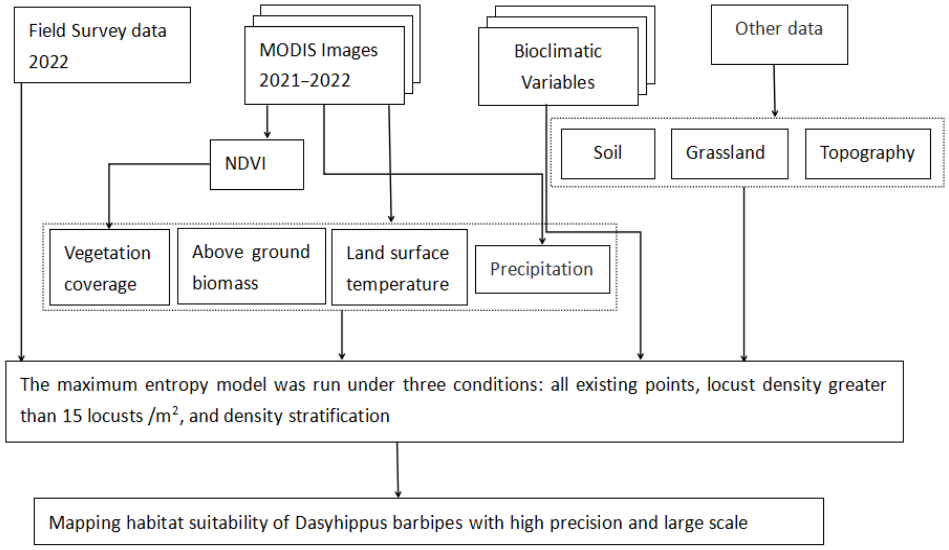
2.2.3. Research Process

The datasets of the field sample points were stratified according to locust distribution density in advance and the low-density, medium-density and medium–high-density datasets were screened out. In the ArcGIS software, the sample points were converted into shp files and then the bioclimatic variables of the sample points were obtained using a multivalue extraction spatial analyst tool. Meanwhile, the hierarchical dataset was input into the Maxent model in batches and the model contribution and correlation were less than 0.8. The bioclimatic variables were screened and input into the Maxent model. The output result was the probability of the occurrence of grassland locusts within the research area. Then, according to the results of the different density levels of the locust sample points and the high-density and all-point data from the conventional methods, the habitat-suitability areas for grassland locusts were identified and compared.
Using ArcGIS, the model calculation results were then reclassified according to the growth of suitable species, with the corresponding ecological factor values when the distribution probability was greater than 0.5. The habitat-suitability areas were identified according to the different density levels and then they were overlaid for analysis. The high-density habitat-suitability areas were selected as the overlapping areas. Thus, the grade distribution map of the habitat-suitability areas for Trichophyta was drawn. The whole research process is shown in Figure 2.

2.2.4. Data Preprocessing

(1)
We imported the downloaded environmental variable data and input the data into the ArcGIS software using a unified geographic coordinate system (WGS84);
(2)
Then, we resampled the data at the same resolution as the bio1 data;
(3)
The data were then cut according to the study area;
(4)
We set the cropped no-data value to −9999;
(5)
Finally, we unified the ranks and numbers of all environmental factors and exported them into ASCII format.

3. Results

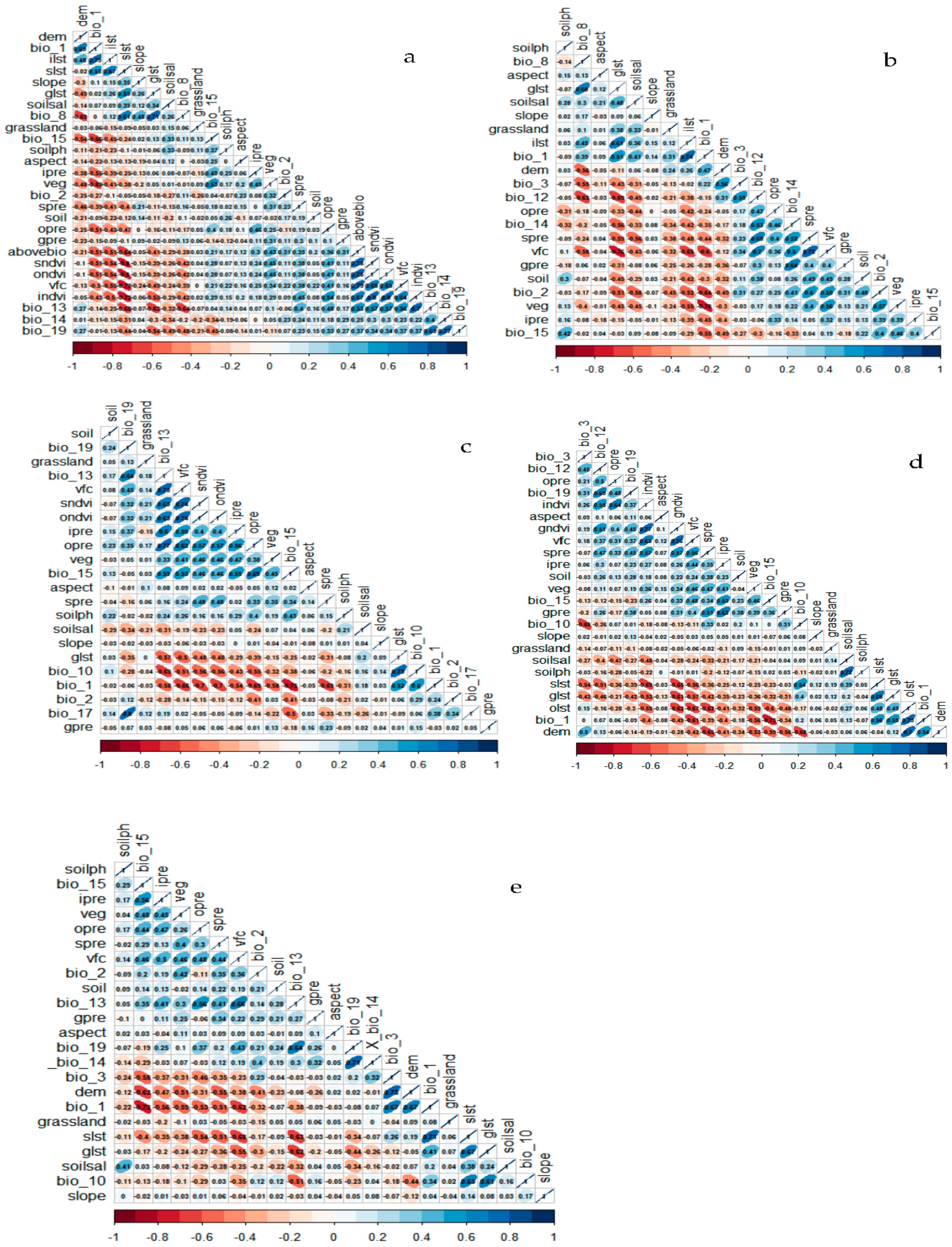
3.1. Filtering the Bioclimatic Variables

Climatic factors are the main factors affecting species distribution. In this study, 41 bioclimatic environmental variables were selected. Because collinearity between variables leads to the overfitting of distribution prediction models, Spearman’s correlation analysis was used to identify the variables with a correlation coefficient of less than 0.8. Those with a correlation coefficient greater than 0.8 were retained and had the largest contribution rate. After filtering, the bioclimatic environmental variables at points 22, 27, 22, 23 and 23 were selected (Table 2) as the dominant variables that affected locust distribution in the grassland areas and were used for our model prediction. The correlation analysis and the removal of highly correlated variables were conducted in R and the corrplot function was used to draw the filtered correlation coefficient matrix. The results are shown in Figure 3.

3.2. Model Training

For our density stratification, all survey sites with a density of more than 15 locusts/m2, the geographical distribution data collected on grassland locusts in Inner Mongolia and the selected bioclimatic variable data were imported into Maxent 3.4.1. Then, 75% of the grassland locust distribution points were randomly selected for model training, with the remaining locust distribution points being used for model verification. During the training process of the model, the AUC evaluation index was used in Jackknife to detect the effects of the model and the importance of each bioclimatic variable in order to verify the accuracy of the model.

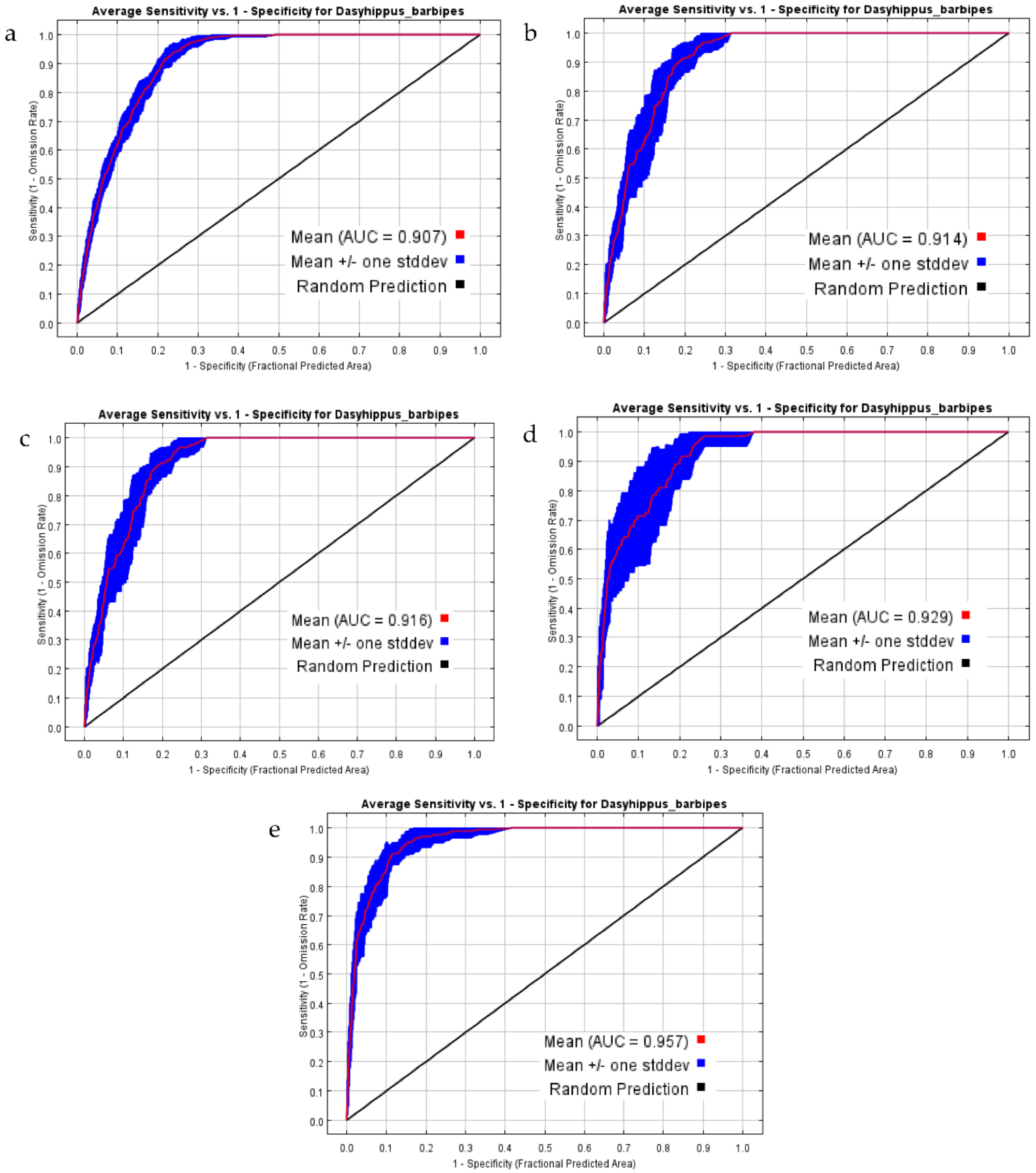
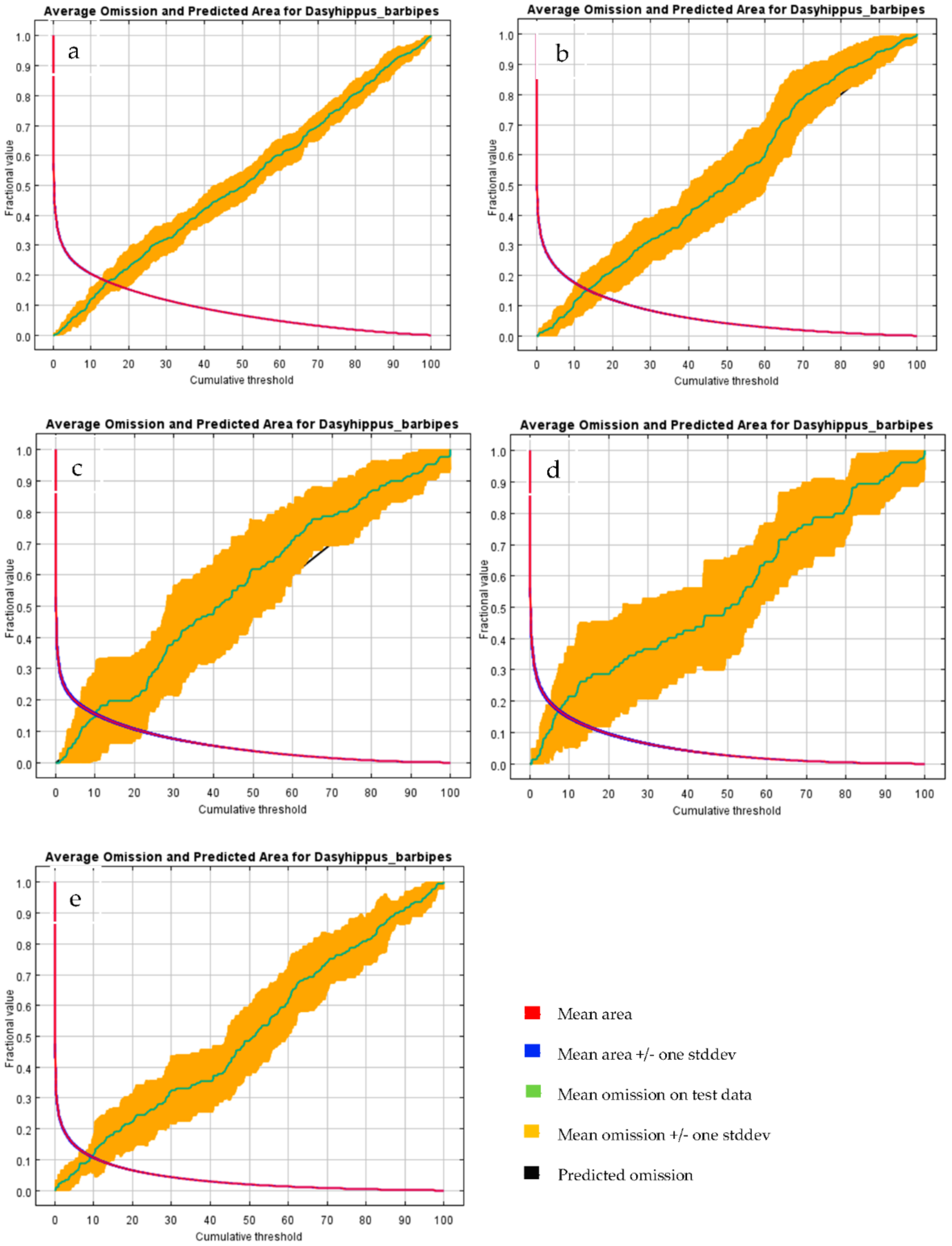
3.3. Maxent Model Verification

To determine the best model, we assessed the quality of the models using the area under the receiver-operating-characteristic curve (ROC) of the test data, i.e., the AUC. The AUC value is between 0.5 and 1.0, with an AUC of 0.5 being assigned for random models and 1.0 for perfect models. The performance of the different models was classified according to their AUC values: 0.5–0.6 = failure; 0.6–0.7 = poor; 0.7–0.8 = common; 0.8–0.9 = good; 0.9–1.0 = excellent (Table 3).
The results showed that the Maxent model had a good AUC value, with an average of 0.907. The average AUC value of the low-density survey points was 0.914, the average AUC value of the low–medium-density survey points was 0.916, the average AUC value of the high–medium-density survey points was 0.929 and the average AUC value of the high-density survey points was 0.957. The different sample-point models had good repeatability and stability. According to the evaluation criteria, the overall prediction accuracy of the models was excellent, indicating that the models were very suitable for simulating the potential distribution of dasyhippus barbipes in the grassland areas of Inner Mongolia. The simulation results are shown in Figure 4.

3.4. Model Evaluation

As can be seen from the function diagrams of the relationships between the omission rate, the probability of occurrence and the cumulative threshold output by the Maxent software (Figure 5), the omission rate of the test set was consistent with the predicted omission rate, indicating that the better the fit between the model and the training data, the more independent the test data and training data.

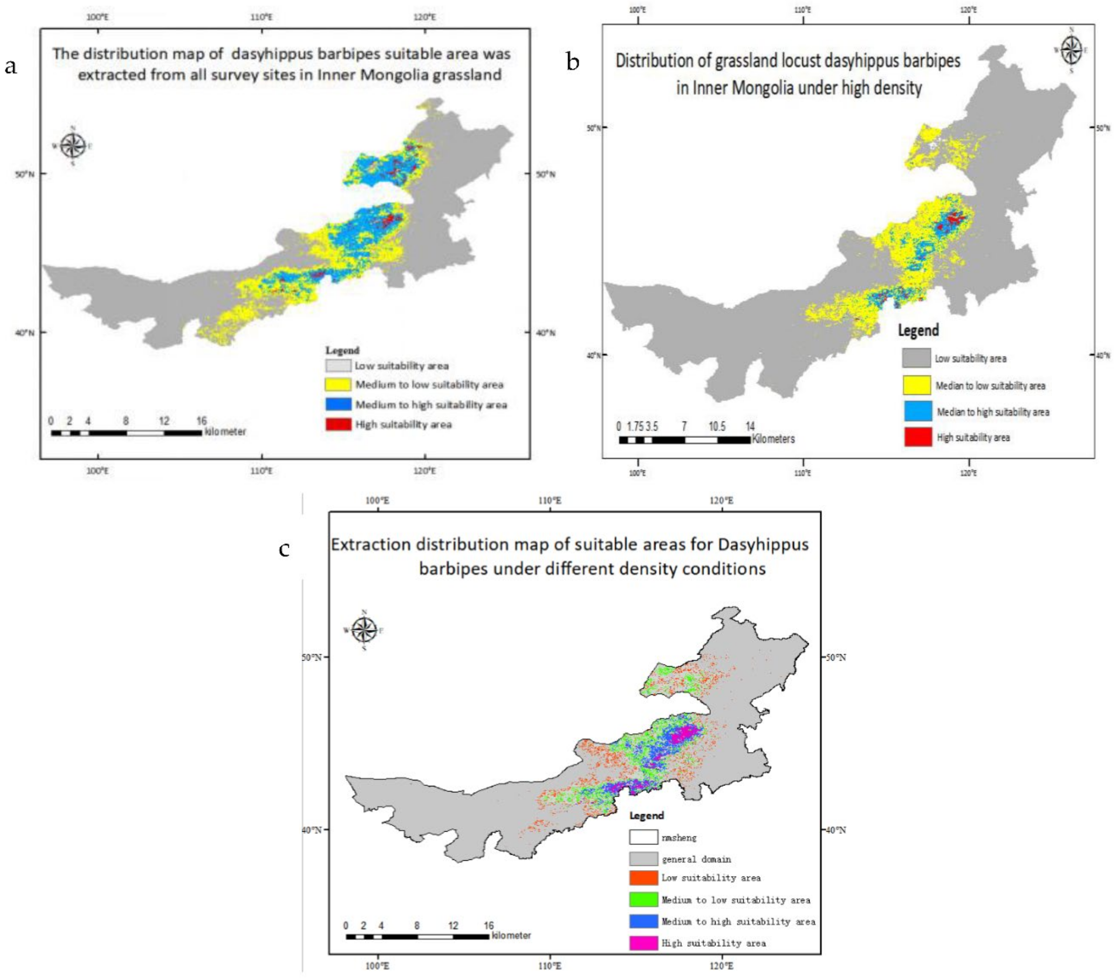
3.5. Distribution and Identification of Habitat-Suitability Areas for the Dominant Species Dasyhippus Barbipes in Inner Mongolia

The output result of the Maxent model was the probability of the occurrence of grassland locusts in the study area. The data were in ASC II format. Firstly, we used the ArcToolbox format-conversion tool in ArcGIS to convert the data into Raster format so that the results could be displayed in ArcGIS. Then, we used the extraction analysis function to obtain the probability distribution map of locusts in the grassland areas of Inner Mongolia. In the expert experience method, the probability of the occurrence of locusts at each grid point (p) was graded according to the research on the identification method for habitat-suitability areas for locusts in Inner Mongolia, where p < 0.05 represented a low-suitability habitat, 0.05 ≤ p <0.33 represented a medium–low-suitability habitat, 0.33 ≤ p < 0.66 represented a medium–high-suitability habitat and p ≥ 0.66 represented a high-suitability habitat [7]. The distribution of the dominant species of grassland locust (Cladochoptera pilipeda) was identified using all survey points and the high-density survey points (i.e., more than 15 locusts/m2), as shown in Figure 6a,b.
When identifying the distributions of the different density levels of habitat-suitability areas for grassland locusts, grid projection was initially carried out using the data-management tool in ArcGIS and then reclassified using the spatial-analysis tool. When the distribution probability was greater than 0.5, its corresponding ecological factor value was suitable for the growth of the species [35]. During the reclassification, the interrupt value was set as 0.5 and the grid operator was used to overlay and analyze the results. During the identification process, we first determined the distribution of high-density grassland locust habitats and then subtracted any overlapping areas of other density classes. Using the same operational method, the low- and medium-density habitat-suitability areas for dasyhippus barbipes were also identified. The results are shown in Figure 6c.
Figure 6. The distribution maps of the dominant species dasyhippus barbipes, based on our maximum entropy model under three scenarios: (a) the extract results using all survey points; (b) the results using the high-density (more than 15 locusts/m2) survey points; (c) the density stratification results.
Remotesensing 15 01718 g006

4. Discussion

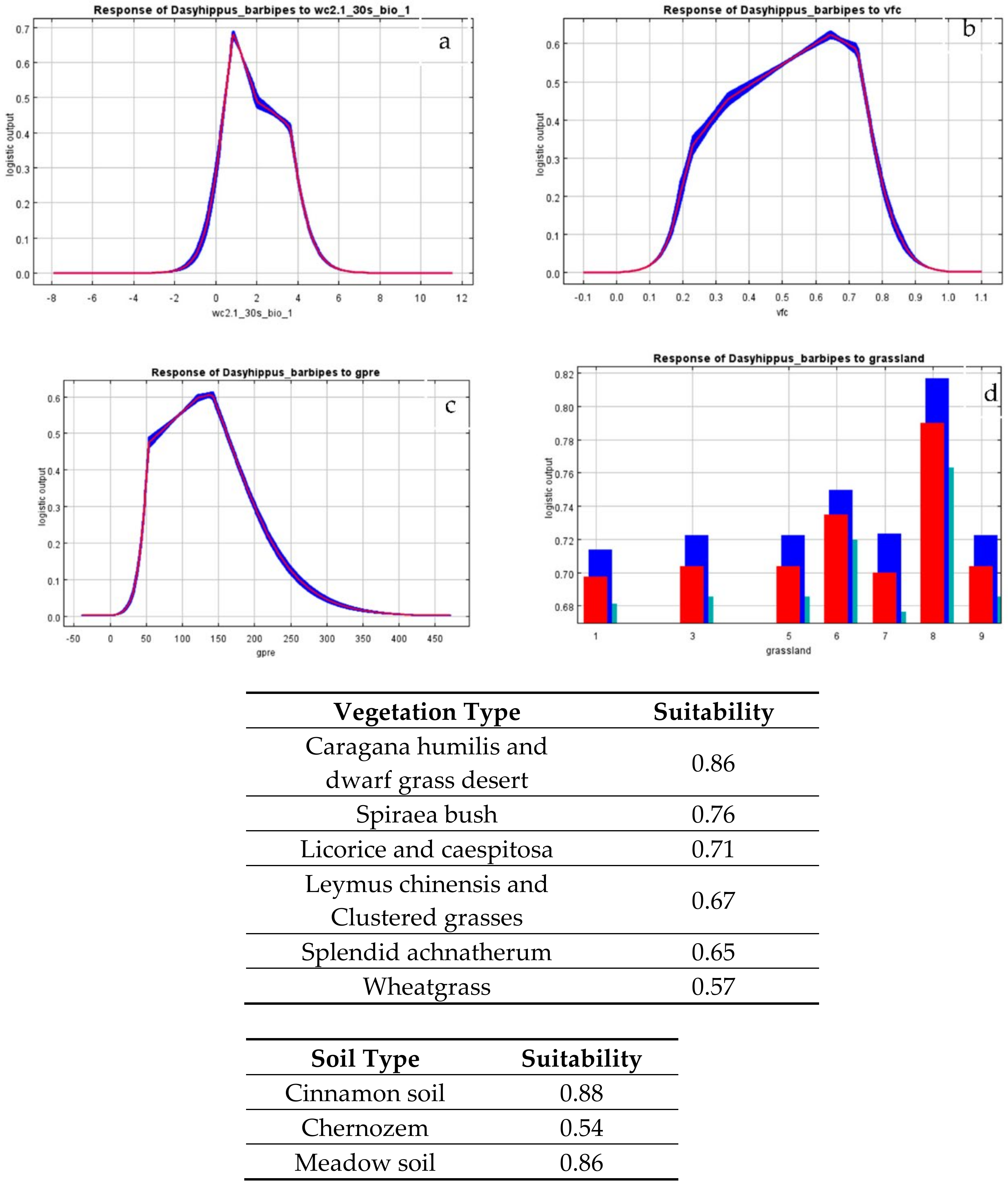
4.1. Response Analysis of the Main Habitat Factors

The Maxent model had two ways to determine the contribution of each environmental factor in the simulation of the geographical distribution of grassland locusts: the percentage contribution and permutation importance, where the percentage contribution was the contribution value of each environmental factor to the geographical distribution of grassland locusts, as given by the Maxent model in the training process, and the permutation importance was the degree to which the AUC value obtained from the model simulation matched that of the real situation after randomly replacing the environmental factors of the training-sample points. The greater the permutation importance, the higher the dependence of the model on that variable.

4.1.1. Response Analysis of the Main Habitat Factors for Locusts in High-Density Grassland Areas

Certain variables, such as bio1, soil, vfc, veg, grassland and gpre, were used to obtain the best model fit in the high-density scenario (Table 4). The following six habitat factors produced the highest independent training gains: mean annual temperature, soil type, vegetation coverage, vegetation type, grassland type and precipitation level in growth season. Figure 7 shows the response curves of these six major habitat factors. The mean annual temperature range was 0.5–2 °C, the soil types were cinnamon, meadow and chernozem and the vegetation coverage was 0.4–0.73. The vegetation types were Caragana humilis, dwarf grass desert, spiraea bush, licorice, cryptosporidium, Leymus chinensis, tufted grass, Achnatherum splendens and ice grass. The grassland types were temperate desert, temperate desertification, other types of grassland, typical temperate grassland, temperate grassland and nongrassland areas. The precipitation level in the growth season was 60–160 mm. These response characteristics were conducive to the spread of the dominant species of grassland locust.

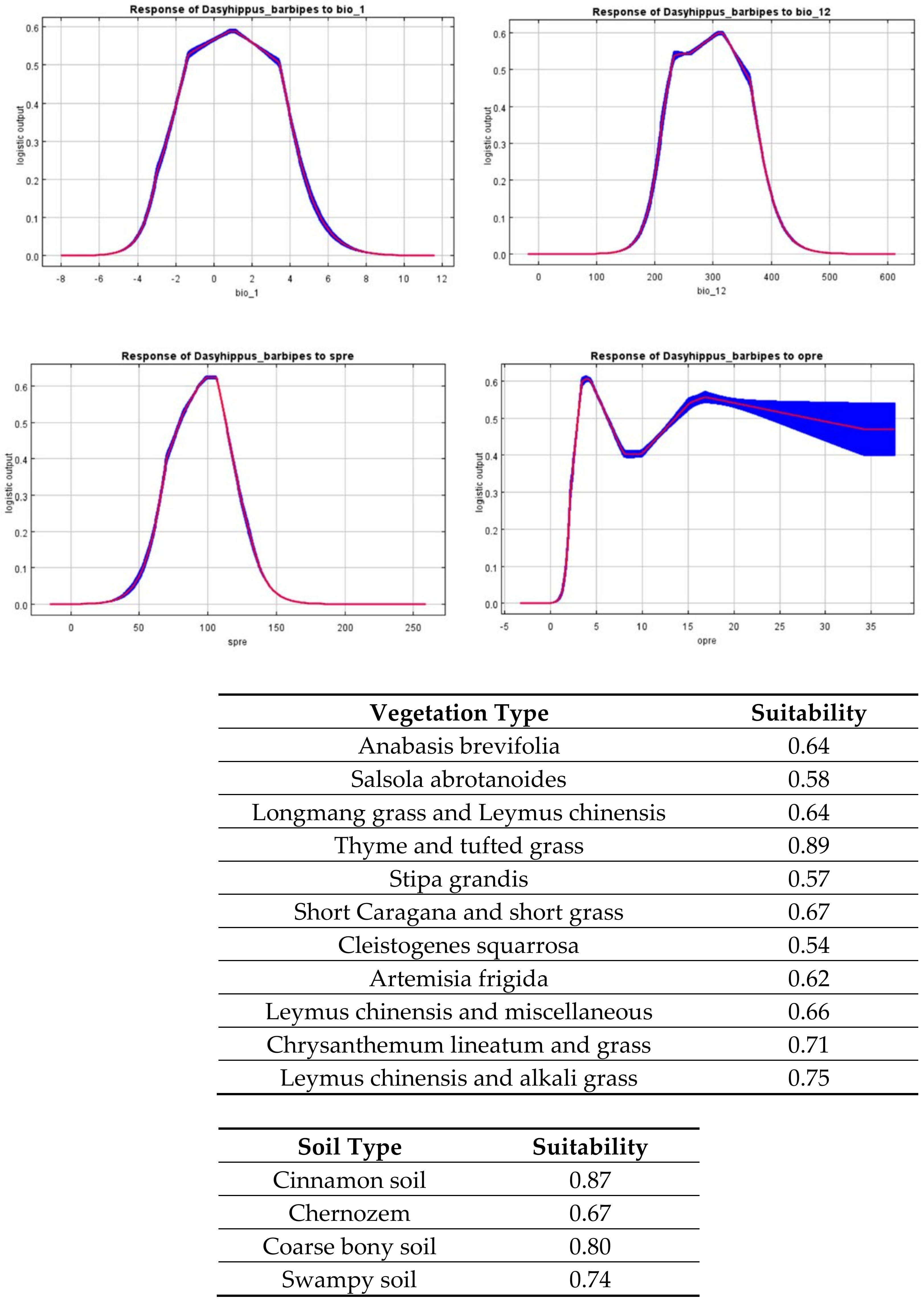
4.1.2. Response Analysis of the Main Habitat Factors for Dasyhippus Barbipes at All Survey Sites

The best model fits for all survey points under the different scenarios were obtained using the bio1, bio12, spre, soil, opre and veg variables (Table 4). The following six habitat factors had the highest independent training gains: mean annual temperature, mean annual precipitation, precipitation level in incubation period, soil type, precipitation level in winter and vegetation type. Figure 8 shows the response curves of these six major habitat factors.
The mean annual temperature range was 1.3–3.5 °C, the mean annual rainfall range was 230–360 mm, the precipitation level in the incubation period was 80–115 mm and the soil types were cinnamon, chernozem, coarse boney and swampy soil. There were two peaks in precipitation levels in the winter period: 3–5 mm and 13–28 mm. The vegetation types were thyme, tufted grass, Leymus chinensis, alkali grass, chrysanthemum linearis, grass, miscellaneous grass, Caragana humilis, dwarf grass, Cryptocarpus scabra, Artemisia frigida, Leymus chinensis, Stipa grandis, pseudowood brevifolia, Salsola artemisiae, Sargassum longifolia, Leymus chinensis and Artemisia annua. These response characteristics were conducive to the occurrence and spread of the dominant species of grassland locust (Rhynchophophora ciliate). The response of dasyhippus barbipes to the main habitat factors in all survey sites was significantly affected by changes in temperature and precipitation, while the response to the main habitat factors in high-density grassland areas was significantly affected by temperature changes.
Figure 7. The response curves of the main habitat factors predicted by our high−density grassland locust dataset model: (a) mean annual temperature; (b) vegetation coverage; (c) precipitation in growth season; (d) grassland type. The response curves show the relationships between the probability of occurrence of locusts and the habitat variables. The displayed values are the average of 10 repeated runs. The blue areas show the ±SD of the 10 repetitions. For each panel, the X axis represents the variable and the Y axis represents the probability of occurrence. Note: the grassland types were classified as follows: 1 = nongrassland area; 3 = other types of grassland; 5 = typical temperate grassland; 6 = temperate desertification; 7 = temperate grassland; 8 = temperate desert; 9 = background value.
Remotesensing 15 01718 g007
Figure 8. The response curves of the main habitat factors in our model prediction, showing the relationships between the probability of the occurrence of locusts and the habitat variables. The displayed values are the average of 10 repeated runs. The blue areas show the ±SD of the 10 repetitions. For each panel, the X axis represents the variable and the Y axis represents the probability of occurrence.
Remotesensing 15 01718 g008

4.1.3. Response Analysis of the Main Habitat Factors for Locusts under Different Density Levels

The response of grassland locusts to the main habitat factors in areas with different density levels is shown in Table 4. The low-density grassland locusts were affected by bio13, bio1, vfc and bio4, whereas other variables, such as oil and ipre, obtained the best model fits. The following six habitat factors produced the highest independent training gains: precipitation level in the wettest month, mean annual temperature, vegetation coverage, temperature variability, soil type, average annual precipitation and precipitation in the incubation period. The best model fit was obtained using bio1, oil, bio13, vfc, spre, veg and other variables in areas with a medium–low density of dasyhippus barbipes. The following six habitat factors produced the highest independent training gains: mean annual temperature, soil type, precipitation in the wettest month, vegetation coverage, monthly average precipitation in the spawning period and vegetation type. The areas with a medium–high density of grassland locusts obtained the best model fits using the variables of soil, bio1, vfc, grassland, dem and veg. The following six habitat factors produced the highest independent training gains: soil type, mean annual temperature, vegetation coverage, grassland type, digital elevation model and vegetation type. The areas with a high density of grassland locusts obtained the best model fits using the bio1, oil, vfc, grassland, veg and gpre variables. The following six habitat factors produced the highest independent training gains: mean annual temperature, soil type, vegetation coverage, grassland type, vegetation type and monthly average precipitation in the growth period.

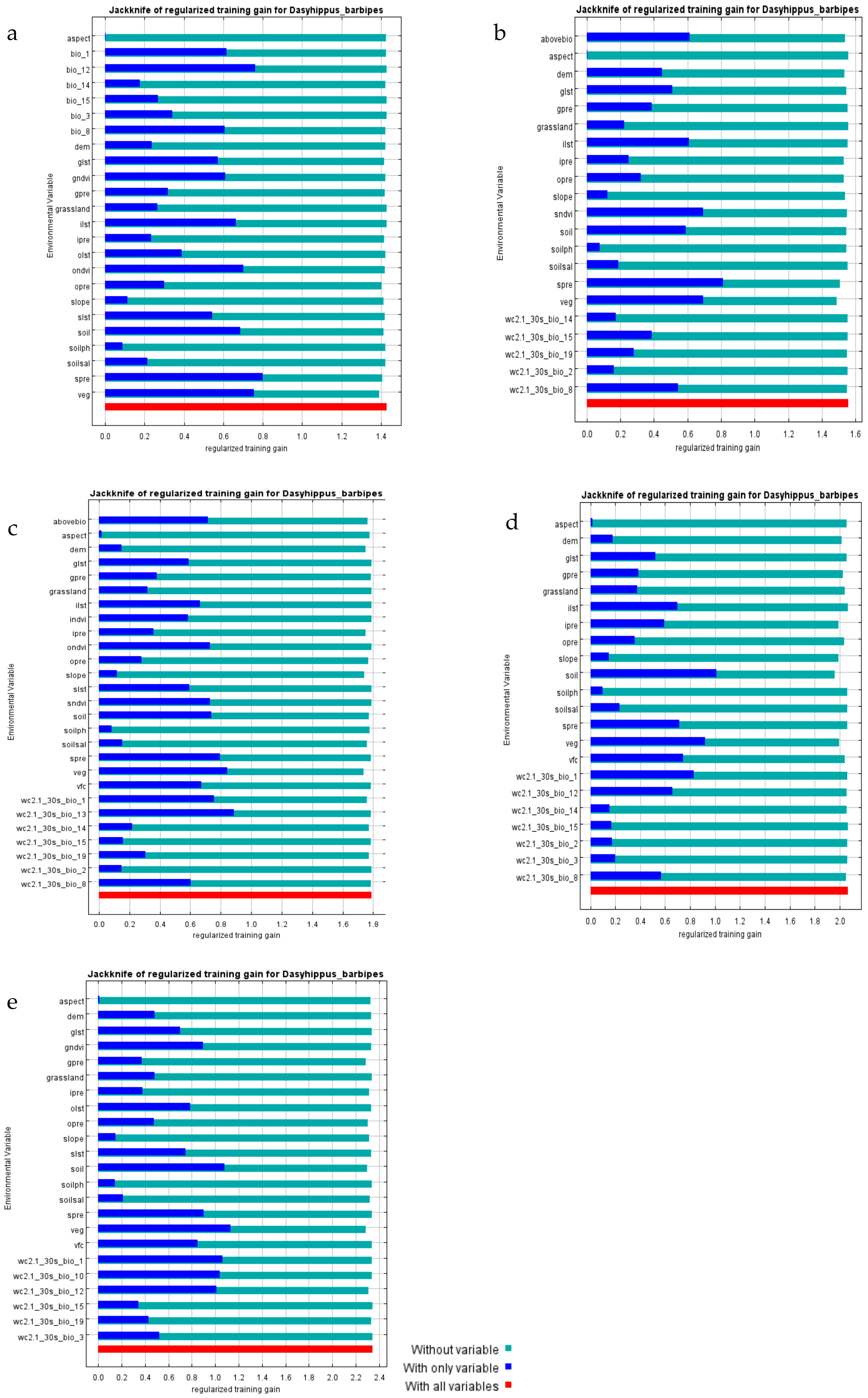
4.1.4. Knife-Cutting Method

The knife-cutting method is similar to cross-validation, in which one or more sample points are excluded at a time and the remaining sample points are used to obtain a corresponding statistic, thereby analyzing the importance of each single variable in the development of a distribution model. Figure 9 shows the importance of each single variable in the development of models for three different scenarios, which were established using the knife-cutting method. For each variable, the red band represents the score of all environmental factors when simulating grassland locust distribution and the dark blue bands indicate the score when only one environmental factor was used to simulate the grassland locust distribution. The higher the score, the more important the climate factor. The light blue bands indicate the score when the other environmental factors were used to simulate the geographical distribution of grassland locusts when that environmental factor was removed. When the difference between the light blue and the dark blue bands was significant, this indicated that the distribution information contained in that climatic factor could not be replaced by other climatic factors and vice versa.

4.2. Difference in Habitat-Suitability Areas for Grassland Locusts under Different Sample Scenarios

The results of the dominant species of grassland locusts in different situations are shown in Table 5, according to the low-, medium–low-, medium–high- and high-suitability areas.
The comparative analysis of the results for the dominant species of grassland locust (Cladochoptera pilipeda) in the three scenarios found that areas with a medium–high and high fitness had a density hierarchy of 95%, which was the same as that of areas with a medium–high and high fitness using the high-density sample data. This was consistent with the research results of Zhongxiang [29,36]. However, there was a large difference between the all-point sample data. When rapidly identifying high-density habitat-suitability areas, the high-density sample-point data could be quickly analyzed with high accuracy, which could provide a favorable means for the rapid and accurate control of locusts.

5. Conclusions

For the first time, we proposed a way to monitor grassland locusts and identify habitat-suitability areas using sample-data-density layering. Through the decorrelation analysis and percentage contribution screening of bioclimatic variables among the sample datasets under various scenarios, the screened environmental variables generally accounted for relatively large proportions of the contribution analysis. Additionally, 70% of the variables had an 80% contribution, such as soil type, vegetation type and other variables. These relatively stable environmental factors could help locust prediction research within the context of future climate models.
In the identification and prediction of habitat-suitability areas for grassland locusts, all-point and high-density methods are often used, and the size and distribution of the sample points have great impacts on the prediction and identification results, thus affecting the large-scale high-quality control of grassland locusts. According to the probability of occurrence of the species, the distributions of different density levels were identified using density stratification, starting from the sample points. The distributions under the three scenarios were explored using data preprocessing, correlation analysis, screening, model inputs and operations and output results, according to their survey geographical locations and environmental variables. The comparative analysis of the habitat-suitability areas for the dominant species of grassland locust (Rhynchophophora ciliate) under the three scenarios found that areas with a medium–high and high fitness had a density hierarchy of 95%, which was the same as that of areas with a medium–high and high fitness using the high-density sample data. The agreement was also good with the actual situation, which demonstrated the significance of the risk assessment of grassland locusts and the timely and accurate prevention and control of locust outbreaks.

Author Contributions

Conceptualization, X.Z. and L.L.; methodology, X.Z. and L.L.; software, X.Z. and L.L.; validation, X.Z.; investigation, X.Z., L.L. and W.H.; data curation, W.H.; Formal analysis, H.Y. and W.H.; writing—original draft preparation, X.Z.; writing—review and editing, X.Z., L.L., H.Y. and. W.H.; supervision, W.H.; funding acquisition, W.H. and H.Y. All authors have read and agreed to the published version of the manuscript.

Funding

This research was funded by the National Key R&D Program of China (Grant No.2021YFE0194800), and the External Cooperation Program of the Chinese Academy of Sciences (Grant No. 183611KYSB20200080), the National Natural Science Foundation of China (Grant No. 42071320), the Alliance of International Science Organizations (Grant No. ANSO-CR-KP-2021-06), the SINO-EU, Dragon 5 proposal: Application of Sino-Eu Optical Data into Agronomic Models to Predict Crop Performance and to Monitor and Forecast Crop Pests and Diseases (Grant No. 57457).

Data Availability Statement

The data are not publicly available because the data needs to be used in future work.

Conflicts of Interest

The authors declare no conflict of interest.

References

  1. Du, G.; Zhao, H.; Tu, X.; Zhang, Z. Study on the division of suitable habitats of Asiatic Locust in Inner Mongolia Grassland. Plant Prot. Res. Rep. 2018, 44, 24–31. [Google Scholar]
  2. Li, G.; Kong, D.; Li, F. Review and prospect of historical locust evolution and water system changes in China. Trop. Geogr. 2017, 37, 226–237. [Google Scholar]
  3. He, K. Habitat Suitability Assessment of Grasshoppers in Inner Mongolia Grassland Based on Multi-Source Remote Sensing Satellite Data. Master’s Thesis, Zhejiang University, Hangzhou, China, 2018. [Google Scholar]
  4. Zhu, M.; Huang, W.; Zhang, R.; Wei, S.; Luo, X.; Yang, Y. Habitat and distribution of grasshopper in Ningxia grassland. J. Plant Prot. 2021, 48, 237–238. [Google Scholar]
  5. Huang, W.; Zhang, J.; Luo, J.; Zhao, J.; Huang, L.; Zhou, X. Monitoring and Forecasting of Crop Diseases and Pests by Remote Sensing; Science Press: Beijing, China, 2015. [Google Scholar]
  6. Liu, L.; Hong, A. Analysis on meteorological and ecological conditions of locust outbreak in Inner Mongolia Grassland in 2004. Atmosphere 2004, 30, 55–57. [Google Scholar]
  7. Li, H.C.; Chen, Y.L. Feeding Habits of Grasshoppers in Typical Steppe of Inner Mongolia, II, Feeding Characteristics in Natural Plant Communities//Study on Grassland Ecosystem, First Episode; Science Press: Beijing, China, 1985; pp. 156–165. [Google Scholar]
  8. Hiekema, J.U.; Roffcy, C.J. Assessment of ecological conditions associated with the 1980/81 desert locust plague upsurge in West Africa using environmental satellite data. Int. J. Remote Sens. 1986, 7, 1609–1622. [Google Scholar] [CrossRef]
  9. Voss, F.; Dreiser, U. Mapping of Desert Locust Habitats using Remote Sensing Techniquest. In New Strategies in Locust Control; Birkhauser: Basel, Switzerland, 1997; pp. 37–45. [Google Scholar]
  10. Gómez, D.; Salvadorect, P. Desert locust detection using Earth observation satellite data in Mauritania. J. Arid. Environ. 2019, 164, 29–37. [Google Scholar] [CrossRef]
  11. Scott, C.A.; Bastiaanssen, W.G.; Ahmad, M.U. Mapping Root Zone Soil Moisture Using Remotely Sensed Optical Imagery. J. Irrig. Drain. Eng. 2003, 129, 326–335. [Google Scholar] [CrossRef] [Green Version]
  12. Lu, S.; Ye, S. Using an image segmentation and support vector machine method for identifying two locust species and instars. J. Integr. Agric. 2020, 19, 1301–1313. [Google Scholar] [CrossRef]
  13. Gómez, D.; Salvador, P.; Sanz, J.; Rodrigo, J.F.; Gil, J.; Casanova, J.L. Prediction of desert locust breeding areas using machine learning methods and SMOS (MIR_SMNRT2) Near Real Time product. J. Arid. Environ. 2021, 194, 104599. [Google Scholar] [CrossRef]
  14. Gómez, D.; Salvador, P. Modelling desert locust presences using 32-year soil moisture data on a Large scale. Ecol. Indic. 2020, 117, 106655. [Google Scholar] [CrossRef]
  15. Taalas, P.; da Silva, J.G. Weather and Desert Locusts; WMO-No.1175; World Meteorological Organization and Food and Agriculture Organization of the United Nations, FAO Desert Locust Information Service: Rome, Italy, 2016. [Google Scholar]
  16. Mamo, D.K.; Bedane, D.S. Modelling the effect of desert locust infestation on crop production with intervention measures. Heliyon 2021, 7, e07685. [Google Scholar] [CrossRef] [PubMed]
  17. Yao, X.; Lu, S.; Gu, J.; Zhang, L.; Yang, J.; Fan, C.; Li, L. A locust remote sensing monitoring system based on dynamic model library. Comput. Electron. Agric. 2021, 186, 106218. [Google Scholar] [CrossRef]
  18. Scanlan, J.C.; Grant, W.E.; Hunter, D.M.; Milner, R. Habitat and environmental factors influencing the control of migratory locusts (Locusta migratoria) with an entomopathogenic fungus (Metarhizium anisopliae). Ecol. Model. 2001, 136, 223–236. [Google Scholar] [CrossRef]
  19. Wang, J.; Du, B.; Gao, S.; Meng, G.; Wang, N.; Lin, K. Research progress in monitoring and warning technology of grasshopper in grassland. J. Plant Prot. 2021, 48, 65–72. [Google Scholar]
  20. Xu, C.; Wang, J. Research progress of integrated locust control technology. J. Plant Prot. 2021, 48, 73–83. [Google Scholar]
  21. Tu, X.; Du, G.; Zhang, Z. Integration and application of green locust control technology system in China. J. Plant Prot. 2021, 48, 1–4. [Google Scholar]
  22. Han, X.; Ma, J.; Luo, J.; Zhang, Y.; Tang, J. Application of remote sensing and GIS in the study of migratory locusts in East Asia. Geogr. Res. 2003, 22, 253–261. [Google Scholar]
  23. Chen, J.; Wang, X. Application of remote sensing and GIS in locust habitat research. J. Ecol. Environ. 2012, 21, 970–976. [Google Scholar]
  24. Chu, X. Tree Species Classification Based on Leaf Non-Imaging Hyperspectral Data. Master’s Thesis, Zhejiang A&F University, Hangzhou, China, 2012. [Google Scholar]
  25. Zhang, J.; Yuan, L.; Wang, J.; Luo, J.; Du, S.; Huang, W. Research progress in remote sensing monitoring of crop diseases and insect pests. Trans. Chin. Soc. Agric. Eng. 2012, 28, 1–10. [Google Scholar]
  26. Jin, R.; Sun, K.; He, H.; Zhou, Y. Research progress of habitat suitability index model. J. Ecol. 2008, 27, 841–846. [Google Scholar]
  27. Zhao, L.; Huang, W.; Chen, J.; Dong, Y.; Ren, B.; Geng, Y. Land use/cover changes in the Oriental migratory locust area of China: Implications for ecological control and monitoring of locust area. Agric. Ecosyst. Environ. 2020, 303, 107110. [Google Scholar] [CrossRef]
  28. Zhao, L. Remote sensing monitoring of temporal and spatial dynamics of locust locust regions in China and its relationship with land use/cover change. Res. Rep. 2019, 1, 1–107. [Google Scholar]
  29. Sun, Z. Study on Extraction of Suitable Habitat Areas of Grassland Locust and Remote Sensing Prediction Method of Occurrence Risk. Ph.D. Thesis, University of Chinese Academy of Sciences, Beijing, China, 2021. [Google Scholar]
  30. Geng, Y.; Zhao, L.; Dong, Y.; Huang, W.; Shi, Y.; Ren, Y.; Ren, B. Migratory Locust Habitat Analysis With PB-AHP Model Using TimeSeries Satellite Images. IEEE Access 2020, 8, 166813–166823. [Google Scholar] [CrossRef]
  31. Saha, A.; Rahman, S.; Alam, S. Modeling current and future potential distributions of desert locust Schistocerca gregaria (Forskål) under climate change scenarios using MaxEnt. J. Asia-Pacifific Biodivers. 2020, 14, 399–409. [Google Scholar] [CrossRef]
  32. Wang, B.; Deveson, E.D.; Waters, C.; Spessa, A.; Lawton, D.; Feng, P.; Liu, D.L. Future climate change likely to reduce the Australian plague locust (Chortoicetes terminifera) seasonal outbreaks. Sci. Total Environ. 2019, 668, 947–957. [Google Scholar] [CrossRef] [PubMed]
  33. Piao, S.L.; Fang, J.Y.; He, J.S.; Xiao, Y. Grassland vegetation biomass and its spatial distribution pattern in China. J. Plant Ecol. 2004, 28, 491–498. [Google Scholar]
  34. Huang, Y.R.; Dong, Y.Y.; Huang, W.J.; Ren, B.; Deng, Q.; Shi, Y.; Bai, J.; Ren, Y.; Geng, Y.; Ma, H. Overwintering distribution of fall armyworm (Spodoptera frugiperda) in Yunnan, China, and influencing environmental factors. Insects 2020, 11, 805. [Google Scholar] [CrossRef]
  35. Yin, X.; Xia, K. Zoology of China. Class Insecta, Orthoptera, Locust Idea: Malleophoridae, Sacroceridae; Science Press: Beijing, China, 2003; Volume 32, pp. 1–340. [Google Scholar]
  36. Liao, J.; Yi, Z.; Li, S.; Xiao, L. Study on the potential distribution of Radix anthomiae in different periods based on Maxent model. Acta Ecol. Sin. 2020, 40, 8297–8305. [Google Scholar]
Figure 2. A flowchart of the research approach.
Remotesensing 15 01718 g002
Figure 3. The correlations between selected variables at different density levels: (a) the low–density correlation coefficient; (b) the medium–low–density correlation coefficient; (c) the medium–high–density correlation coefficient; (d) the high–density correlation coefficient; (e) the all–points correlation coefficient.
Remotesensing 15 01718 g003
Figure 4. The average AUC values of the different density scenarios: (a) all survey points; (b) the low-density survey points; (c) the low–medium-density survey points; (d) the medium–high-density survey points; (e) the high-density survey points.
Remotesensing 15 01718 g004
Figure 5. The relationships between the omission rate, occurrence probability and cumulative threshold at different density levels: (a) all survey points; (b) the low-density survey points; (c) the medium–low-density survey points; (d) the medium–high-density survey points; (e) the high-density survey points.
Remotesensing 15 01718 g005
Figure 9. The results of the knife-cutting test for the importance of the environmental variables in the Maxent model at different density levels: (a) all survey points; (b) the low-density survey points; (c) the medium–low-density survey points; (d) the medium–high-density survey points; (e) the high-density survey points. The environment variables in this figure have the same meanings as those shown in Table 1.
Remotesensing 15 01718 g009
Table 1. The environmental climate variables in our Maxent model.
Variable and DescriptionUnit
bio1, Mean Annual Temperature°C
bio2, Mean Diurnal Range (i.e., mean of monthly (max. temp.–min. temp.))°C
bio3, Mean Annual Temperature Range (i.e., bio2/bio7 × 100)%
bio4, Temperature Seasonality°C
bio5, Max. Temperature of Warmest Month°C
bio6, Min Temperature of Coldest Month°C
bio7, Annual Temperature Range (i.e., bio5–bio6)°C
bio8, Mean Temperature of Wettest Quarter°C
bio9, Mean Temperature of Driest Quarter°C
bio10, Mean Temperature of Warmest Quarter°C
bio11, Mean Temperature of Coldest Quarter°C
bio12, Annual Precipitationmm
bio13, Precipitation Level in Wettest Monthmm
bio14, Precipitation Level in Driest Monthmm
bio15, Precipitation Seasonality (i.e., coefficient of variation)%
bio16, Precipitation Level in Wettest Quartermm
bio17, Precipitation Level in Driest Quartermm
bio18, Precipitation Level in Warmest Quartermm
bio19, Precipitation Level Coldest Quartermm
soil, Soil Typecategorization
soilph, Soil AcidityPH
soilsal, Soil SalinitydS/m
grassland, Grassland Typecategorization
veg, Vegetation Typecategorization
vfc, Vegetation Coverage%
abovebio, Aboveground Plant Coveragekg/m2
dem, Digital Elevation Modelm
Slope°
Aspect°
spre, Mean Monthly Precipitation in Growth Periodmm
slst, Mean Monthly Temperature in Growth Period°C
sndvi, Mean Monthly Vegetation Index in Growth Period%
gpre, Mean Monthly Precipitation in Growth Periodmm
glst, Mean Monthly Temperature in Growth Period°C
gndvi, Mean Monthly Vegetation Index in Growth Period%
ipre, Mean Monthly Precipitation in Incubation Periodmm
ilst, Mean Monthly Temperature in Incubation Period°C
indvi, Mean Monthly Vegetation Index in Incubation Period%
opre, Mean Monthly Precipitation in Wintermm
olst, Mean Monthly Temperature in Winter°C
ondvi, Mean Monthly Vegetation Index in Winter%
Table 2. The filtered results of the different density levels of the environmental variables.
Low DensityMedium-to-Low DensityMedium-to-High DensityHigh DensityAll Points
aspectabovebioaspectaspectaspect
glstaspectdemdemdem
gpredemglstglstglst
grasslandglstgpregndvigpre
ipregpregrasslandgpregrassland
ondvigrasslandilstgrasslandipre
opreilstipreipreopre
slopeindviopreolstslope
sndviipreslopeopreslst
soilondvisoilslopesoil
soilphopresoilphslstsoilph
soilsalslopesoilsalsoilsoilsal
spreslstspresoilphspre
vegsndvivegsoilsalveg
vfcsoilvfcsprevfc
bio1soilphbio1vegbio1
bio2soilsalbio2vfcbio2
bio10sprebio3bio1bio3
bio13vegbio8bio10bio10
bio15vfcbio12bio12bio13
bio17bio1bio14bio15bio14
bio19bio2bio15bio19bio15
bio8 bio3bio19
bio13
bio14
bio15
bio19
Table 3. The AUC values for our model accuracy verification.
AUC ValueModel Results
<0.5Failed to describe reality
0.5Random distribution
0.5–0.6Failed
0.6–0.7Poor
0.7–0.8Common
0.8–0.9Good
>0.9Excellent
Table 4. The response variables, percentage contributions and permutation importance of the major habitat factors under the three scenarios.
DensityVariablePercentage ContributionPermutation ImportanceDensityVariablePercentage ContributionPermutation Importance
Lowbio_1316.519.6Medium–Lowbio_121.628
bio_114.20.9soil15.50.7
vfc12.42.5bio_1311.93.1
bio_411.50.3vfc10.32.7
soil50.9spre8.24.5
ipre4.94.8veg5.44.5
Medium–Highsoil26.94.3Highbio_124.94.8
bio_120.510.8soil20.12.5
vfc11.86.1vfc11.80.8
grassland7.60.5grassland7.20.3
dem620.9veg6.92.8
veg5.74.9gpre5.59.8
All Pointsbio_1323.317.1
bio_121.59.1
vfc135.2
soil11.12.2
spre6.17.9
veg5.84.1
Table 5. The results for the habitat-suitability areas for grassland locusts under different scenarios.
Sample Point TypeDegree of FitnessHabitat-Suitability Area (km2)
All pointsLow301,810
Medium–Low229,331
Medium–High180,940
High12,647
Greater than 15 locusts/m2Low217,976
Medium–Low173,141
Medium–High46,283
High7318
Different density classesLow57,344
Medium–Low55,855
Medium–High32,242
High23,934
Disclaimer/Publisher’s Note: The statements, opinions and data contained in all publications are solely those of the individual author(s) and contributor(s) and not of MDPI and/or the editor(s). MDPI and/or the editor(s) disclaim responsibility for any injury to people or property resulting from any ideas, methods, instructions or products referred to in the content.

