A Partial Reconstruction Method for SAR Altimeter Coastal Waveforms Based on Adaptive Threshold Judgment

Abstract

Due to land contamination and human activities, the sea surface height (SSH) data retrieved from altimeter coastal waveforms have poor precision and cannot provide effective information for various tasks. The along-track high-resolution characteristic of the new synthetic aperture radar (SAR) altimeter makes the retracking methods of traditional coastal waveforms difficult to apply. This study proposes a partial reconstruction method for SAR altimeter coastal waveforms. By making adaptive threshold judgments of model matching errors and repairing the contaminated waveforms based on the nearest linear prediction, the success rate of retracking and retrieval precision of SSH are significantly improved. The data from the coastal experimental areas of the Sentinel-3B satellite altimeter are processed. The results indicate that the mean proportion of waveform quality improvement brought by partial reconstruction is 80.30%, the mean retracking success rate of reconstructed waveforms is 85.60%, and the mean increasing percentage is 30.98%. The noise levels of SSH data retrieved by different methods are calculated to evaluate the processing precision. It is shown that the 20 Hz SSH precisions of the original and reconstructed coastal waveforms are 12.75 cm and 6.32 cm, respectively, and the corresponding 1 Hz SSH precisions are 2.85 cm and 1.41 cm, respectively. The results validate that the proposed partial reconstruction method has improved the SSH precision by a factor of two, and the comparison results with mean sea surface (MSS) model data further verify this conclusion.

1. Introduction

Satellite radar altimeters are advanced remote sensing equipment that can effectively observe the global marine environment all day and in any weather condition [1]. By retracking the altimeter waveform, important parameters, such as the sea surface height (SSH), significant wave height (SWH), backscattering coefficient, and wind speed, can be retrieved [2]. To further improve observation accuracy and spatial resolution, satellite radar altimeters have gradually evolved from real to synthetic aperture systems, providing long-term and high-quality ocean measurement results for decades [3]. At this stage, the 1 Hz height measurement precision of the traditional radar altimeter (such as Poseidon-3B carried by the Jason-3 satellite) in the open ocean can be better than 2 cm (SWH = 2 m) [4]. The along-track resolution of the synthetic aperture radar (SAR) altimeter (such as the SAR altimeters carried by the Sentinel-3 satellite and Jason-CS satellite) is approximately 300 m [5,6], and the 1 Hz height measurement precision in the open ocean can reach approximately 1 cm (SWH = 2 m) [7,8]. These high-precision observations have significantly promoted the development of marine science.

Nevertheless, the SSH measurement precision of satellite radar altimeters in coastal areas remains low for two main reasons. First, the beam coverage of spaceborne radar altimeters is very large, typically in the range of 10–20 km. Therefore, when the offshore distance of the subsatellite point is within 10 km, the land reflection signal interferes with the radar echo, causing the altimeter waveform to deviate from the standard form of the ocean echo [9,10,11]. In addition, many ports, airports, ships, and islands are scattered throughout the coastal area, which aggravates the degree of contamination of the coastal waveform. In this case, performing retracking based on the theoretical model of ocean echo will inevitably lead to large errors in the ranging results, resulting in the low retrieval precision of the SSH [12,13]. Second, the correction items of altimeter height measurement, such as the wet tropospheric component, ocean tide, sea state bias, and inverse atmospheric pressure, are of poor quality in near-shore areas, and the measurement accuracies are much worse than those in open-ocean areas [14,15]. Therefore, most current studies use grid data extrapolated from the open ocean to the coastal zone [16]. Such data can only reflect a theoretical gradual change trend but cannot be used to observe or reveal new coastal physical phenomena.

However, coastal areas are most directly related to human activities, and changes in SSH are closely interrelated with climate prediction, ship navigation, and fishery production. Traditional single-point and single-route hydrological measurement methods, such as buoys, mooring arrays, and ship surveys, have very limited measurement ranges and time efficiency. Thus, they are far from providing large-area, long-term data for studying the temporal and spatial changes of the sea surface. The satellite radar altimeter, on the other hand, has the above observation ability and has accumulated decades of measurement data, including a large number of coastal waveforms, which still contain a lot of valuable information. Therefore, many institutions and scholars have begun to study the processing method of altimeter coastal waveforms to improve the usable proportion and retrieval precision of coastal data and better serve human activities.

Altimeter-based investigations in Corsica, Capraia, and the Contiguous Area (ALBICOCCA) and Altimetry for Coastal Regions (ALTICORE) projects were jointly initiated by France, Italy, and the United Kingdom in 2001 and 2006, respectively [17]. These two projects aim to study the altimeter data processing method suitable for coastal areas by establishing regional tidal and inverse atmospheric pressure models and combining the orbit correction of multiple satellites. However, these two projects only considered the measurement accuracies of the correction terms in nearshore water bodies and did not study the waveform of the altimeter itself. To solve the problems of altimetry height measurements in coastal areas and generate available coastal products, the Centre National d’Etudes Spatiales (CNES) initiated the PISTACH project based on the Jason-2 satellite [18]. In this project, altimeter waveforms are divided into 16 types through a neural network algorithm, and four different retracking methods are used for follow-up processing, which improves the retrieval precision of coastal data to a certain extent.

Additionally, many scholars have proposed specific processing methods for altimeter coastal waveforms. These methods can be divided into three categories: The first type is the total waveform retracking method, which can be subdivided into model-based (physical) and empirical-based algorithms. The former, such as the ocean algorithm [19], Beta 5/9 algorithm [20], and Ice-2 algorithm [21], have a high calculation accuracy owing to iterative processing. However, the precondition is that the waveform characteristics conform to the model definition; otherwise, it can easily fail. The latter, such as the offset center of gravity (OCOG) [22] and threshold [23] algorithms, are more robust, with faster calculation speed but lower accuracy. The second type is the machine-learning method, which includes three main steps [24,25]. First, some waveform characteristics are manually defined; then, altimeter waveforms are classified based on the neural network algorithm; and finally, different model- or empirical-based algorithms are used to perform retracking. The third type is the sub-waveform retracking method, the key to which is extracting the correct sub-waveform. Representative methods include the multi-peak sub-waveform retracking algorithm [26] and the adaptive leading edge sub-waveform (ALES) algorithm [27,28,29]. The ALES algorithm was initially proposed to process the traditional altimeter waveforms [27] and then extended to process the SAR altimeter waveforms [29]. However, its echo model still adopts the Brown model and has not been improved to the SAR echo model. Moreover, based on the assumption that the primary peak of the waveform is the water surface signal, Jain et al. [30] proposed a narrow primary peak retracking (NPPR) algorithm to process the SAR altimeter data of the Cryosat-2 satellite.

In general, these methods have their own advantages, and their processing effects for specific types of waveforms have been improved. However, except for empirical algorithms and the NPPR algorithm, other algorithms have mostly been proposed for traditional altimeter waveforms, and their applicability to SAR altimeter coastal waveforms remains to be verified. In addition, the along-track high-resolution characteristic of the SAR altimeter makes the waveform present a narrow peak; therefore, it is difficult to extract a sectional, uncontaminated sub-waveform. Based on the above analysis, this study proposes a partial reconstruction method for SAR altimeter coastal waveforms, which significantly improves the success rate of retracking and retrieval precision of SSH.

In Section 2, the satellite dataset and the experimental areas are introduced. The vital steps of the coastal waveform processing method are studied afterwards, mainly including echo model fitting, matching error calculation, adaptive threshold judgment, and nearest waveform reconstruction. The NPPR algorithm for precision comparison is illustrated at the end. In Section 3, the retracking results of the coastal waveforms are presented. The retracking success rates before and after reconstruction are then compared. Finally, the retrieval precisions of SSH data obtained by different methods are calculated and validated based on the mean sea surface (MSS) model. Section 4 concludes the study.

2. Materials and Methods

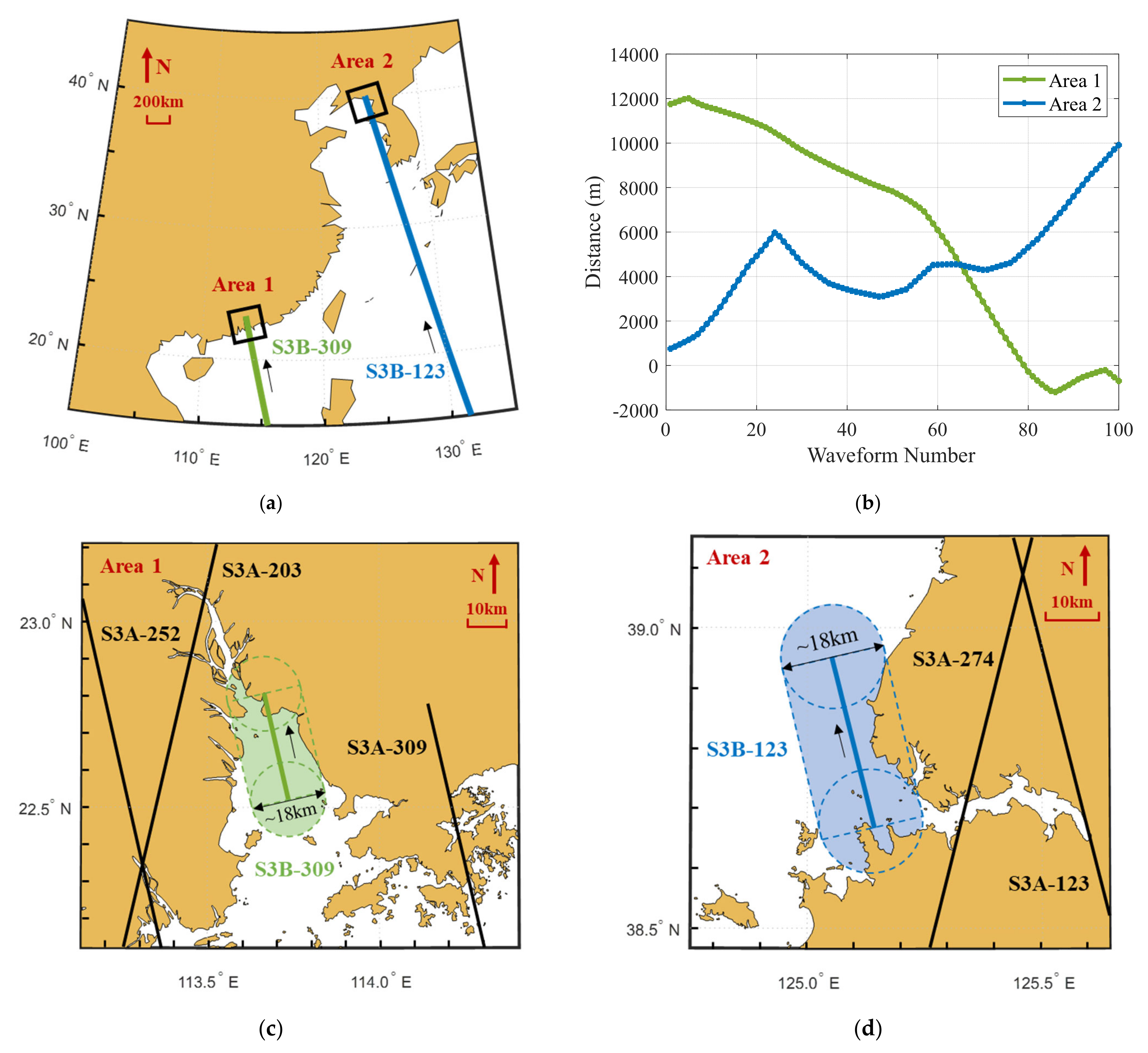
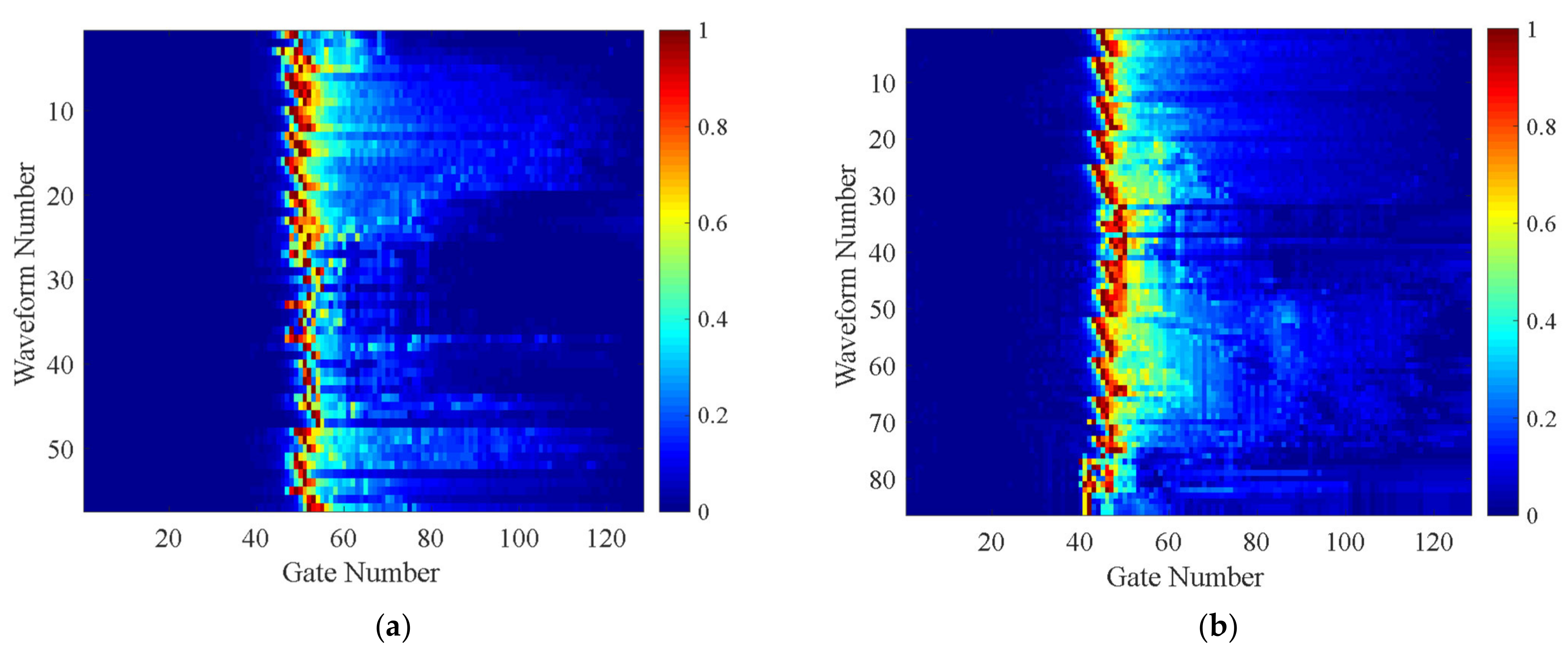
2.1. Coastal Waveform Data of the Sentinel-3 SAR Altimeter

To collect high-quality, long-term ocean, land, and atmospheric information, the European Commission and the European Space Agency jointly initiated the Global Monitoring for Environment and Security program, including the development of the Sentinel-3 satellite for the Earth Observation project [31]. The Sentinel-3 mission consists of A/B satellites launched on 16 February 2016, and 25 April 2018, respectively. Sentinel-3A is equipped with the SAR altimeter (SRAL), which operates in SAR mode on a global scale for the first time. Sentinel-3B has an identical orbit design and load composition as Sentinel-3A but flows 180° out of phase with 3A [32]. The SAR mode measurement data of the two satellite altimeters were both subjected to long-term quality monitoring.

The two black boxes in Figure 1a represent the two experimental areas selected for this study. Experimental area 1 is located in the nearshore of the South China Sea, and experimental area 2 is located in the nearshore of the West Korean Gulf. In the figure, the yellow part represents land, and the white part represents the ocean. The green and blue lines represent the subsatellite tracks, which correspond to passes 309 and 123 of Sentinel-3B, and the two black arrows represent the satellite’s flight directions. Figure 1b shows the offshore distances of the subsatellite points in the two experimental areas, which are mainly concentrated within 10 km of the coastal area. The distance data are obtained from the L2 geographical data record (GDR) of satellite products, which are downloaded from the EUMETSAT Data Store [33], and a negative number indicates that the satellite has entered land. Figure 1c,d show the coastal details of the two experimental areas. The light green and blue areas within the dotted lines represent the coverage of the altimeter beam. The diameter of the radar beam was approximately 18 km, which was calculated using the satellite system parameters. Since the two experimental areas are located near ports, where human activities are intensive and the probability of ship occurrence is high, the altimeter echo will not only be contaminated by land but also be affected by ships. Additionally, there are also differences between the two experimental areas. For area 1, the altimeter measures from the sea to the land, and the along-track direction is gradually contaminated. For area 2, the altimeter measures from land to sea, and there is continuous land contamination in the cross-track direction. The different measurement features of the two experimental areas can better test the robustness and accuracy of the proposed method. Figure 1c,d also show several passes of Sentinel-3A in the experimental areas (black lines). It can be seen that, due to the sparse sampling of satellites, the tracks of Sentinel-3A in these two areas do not pass the coastal regions; therefore, Sentinel-3B altimeter data are selected for processing.

The data used in this study were obtained from the L2 GDR product of Sentinel-3B. The dataset information for the two experimental areas is listed in

Table 1. Dataset information for experimental areas used for coastal waveform processing.

Item	Area 1	Area 2
Measure Satellite	Sentinel-3B
Measure Mode	SAR
Measure Year	2022
Measure Pass	309	123
Measure Month	3, 4, 6, 7, 9	a whole year
Data Rate	20 Hz
Data Level	L2 GDR

. For experimental area 1, the measurement data from pass 309 in five months of 2022 were selected. As area 1 is used for testing the effectiveness of the proposed reconstructive method step by step, the waveforms of the selected months are seriously contaminated and deviate significantly from the standard ocean shape. Then, the reconstructive method was applied to the measurement data of area 2, which corresponded to pass 123, and the time span was a whole year of 2022. Since Sentinel-3B adopts a repeated orbit design with a period of approximately 27 days, the subsatellite tracks in different months almost coincide. The sampling rate of the data is 20 Hz, and 100 continuous waveforms are selected from each pass. The corresponding measurement time was approximately 5 s, and the satellite flight distance was approximately 35 km. Figure 2a–d show the normalized coastal waveforms of the two areas in different months, and the normalization is achieved by dividing the maximum value of the waveform. It can be seen that, owing to the complex nearshore terrain and intensive human activities, the echo shapes change dramatically even in the almost coincident geographical location.

Figure 3 shows typical coastal waveforms in the experimental area, in which the amplitudes are normalized by dividing the maximum values of the waveforms. It can be observed that the shapes of the waveforms are very different. Figure 3a shows a sharp single-peak waveform, which means that the observing surface is rather smooth, such as a calm lake or flat ice. Figure 3b shows a double-peak waveform, which means that there are targets slightly farther away from the radar altimeter that have stronger scattering characteristics than seawater, such as metal ships, aircraft, or buildings, assuming that the first peak corresponds to the seawater. The waveform in Figure 3c contains multiple peaks, which means that the targets in the observation range are more complicated. The waveform in Figure 3d is slightly contaminated but can still distinguish the ocean echo form, which means that the edge of the beam may be covering part of the land. Yet the waveforms in Figure 3e,f are heavily contaminated and can hardly distinguish the ocean form, which means that the complicated coastal topography has distorted the waveforms severely. It has been concluded from the previous introduction that the processing methods of the altimeter total waveform can be divided into two categories: empirical-based algorithms, such as classic OCOG retracking, and model-based physical waveform retracking. The former has strong robustness but poor accuracy, whereas the latter has high accuracy but poor adaptability. To improve the retrieval precision of coastal SSH data, this study adopted the processing idea of model-based physical waveform retracking. The main reason for the failure of model fitting is that there is a large difference between the actual coastal waveform and the theoretical echo model. Therefore, this study proposes a partial reconstruction method applied to SAR altimeter coastal waveforms. By improving the matching degree between the waveform and model, the success rate of retracking and SSH retrieval precision increases remarkably.

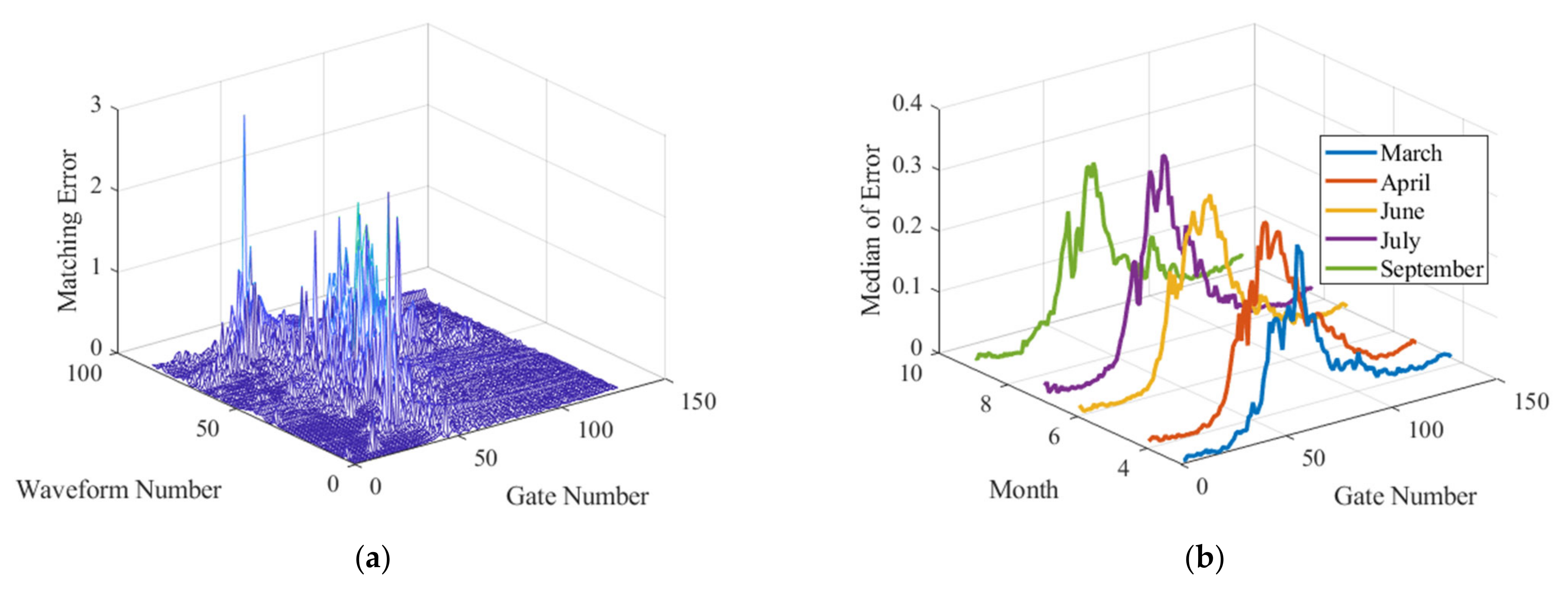
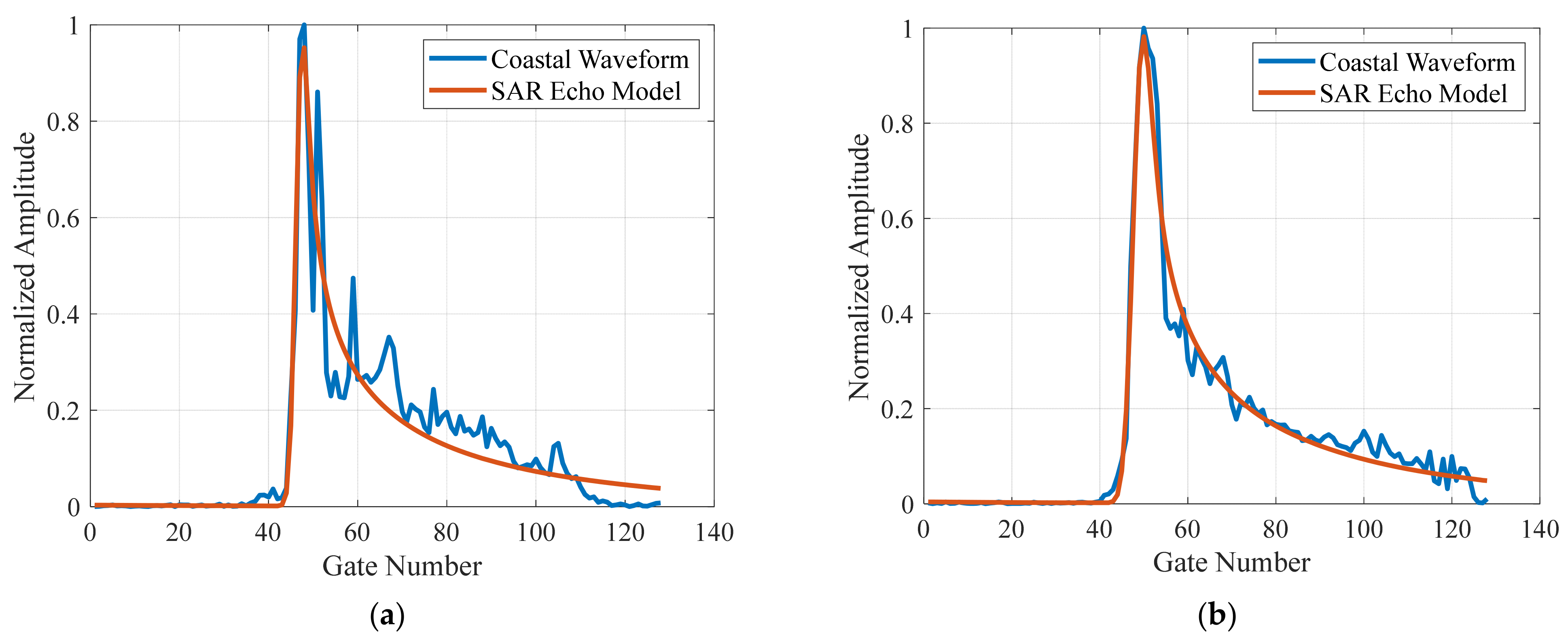
2.2. Echo Model Fitting and Matching Error Calculation

In 1977, Brown proposed an explicit expression of the sea surface backscatter echo model for radar altimeters [12]:

$$P(t)=P_{FS}(t)\ast q_s(t)\ast s_r(t);$$

(1)

where $P(t)$ is the average power of the received echo, $P_{FS}(t)$ is the impulse response function of the flat sea surface, $q_s(t)$ is the probability density function of surface wave height, and $s_r(t)$ is the point target response of radar system.

The echo model of the SAR altimeter is established based on the Brown model, in which:

$$q_s(t)=\frac{1}{\sqrt{2\pi }{\sigma }_s}\exp (-\frac{t^2}{2{\sigma }_s^2});$$

(2)

$$s_r(t)=\frac{1}{\sqrt{2\pi }{\sigma }_p}\exp (-\frac{t^2}{2{\sigma }_p^2});$$

(3)

where ${\sigma }_s=\frac{\mathrm{SWH}}{2c}$, $c$ is the light speed, SWH is the significant wave height, ${\sigma }_p=1.125/B$, $B$ is the bandwidth of the radar transmitting signal.

Let ${\sigma }_c=\sqrt{{\sigma }_p^2+{\sigma }_s^2}$, then the convolution of the above two functions is:

$$Y(t)=\frac{1}{\sqrt{2\pi }{\sigma }_c}\exp (-\frac{t^2}{2{\sigma }_c^2});$$

(4)

For the SAR altimeter, the along-track echoes are processed using synthetic aperture technique. Therefore, the radar beam has been sharpened, and the real aperture beam is divided into several along-track sub-beams [34]. Each sub-beam corresponds to a Doppler strip along the flight track, and the strip width determines the azimuth resolution of the SAR altimeter. Due to the relative velocity variation from the aircraft to the along-track strips, the echoes from different strips have different Doppler frequencies, which are called sub-look echoes. The sub-look echoes are performed with range migration correction to compensate the range migration produced by the motion of the sensor along the orbit with respect to each surface strip and improve the signal-to-noise ratio, and accumulated incoherently afterwards to obtain the multi-look echo, which is the SAR waveform [35].

Based on the above processing procedure, it can be concluded that the steps of establishing the SAR echo model are as follows: firstly, establishing single-look $P_{FS}(t)$ for each strip according to the Doppler frequencies, then convolving $P_{FS}(t)$ with $Y(t)$ to obtain the single-look model, and finally performing multi-look processing [36,37].

To determine the impulse response function of the flat sea surface is the most challenging part, and many SAR altimeter echo models are established based on different approximate conditions [38,39]. Liu et al. [40] propose a high-precision SAR altimeter echo model. In this study, coastal waveform data are processed using this model. When the total number of accumulated looks is $M$, the echo model can be expressed as:

$$P(t)={\displaystyle \sum _{i=1}^M{P}_i(t)};$$

(5)

$$P_i(t)=Y(t-\tau )\ast P_{FS}^i(t);$$

(6)

$$P_{FS}^i(t)=\frac{{\lambda }^2{G}_0^2{D}_{0}c{\sigma }^0}{32{\pi }^2{H}^3\eta }\cdot J(t+\frac{\eta H{\xi }_k^2}{c})\cdot {\displaystyle \underset{0}{\overset{2\pi }{\int }}F}({\rho }_{k}cos\vartheta -{\xi }_k)\cdot G({\rho }_k,\vartheta )d\vartheta ;$$

(7)

where $P_i(t)$ is the single-look echo model, $\tau$ is the echo epoch, and $P_{FS}^i(t)$ is the single-look impulse response function. The meanings of the physical quantities in Equation (7) are consistent with those in Ref. [40].

The echo model of the SAR altimeter includes three parameters: the epoch, SWH, and amplitude. The epoch corresponds to the half-power point on the leading edge, based on which the SSH can be retrieved; the SWH corresponds to the slope of the rising edge; and the amplitude can be used to calculate the backscattering coefficient. Waveform retracking uses a certain mathematical method (usually the least-squares algorithm) to fit the echo model with the actual waveform to obtain the best parameter results [41,42].

The processing steps of SAR altimeter coastal waveforms are described as follows.

Step 1: Thermal noise removal. The gate range corresponding to the noise region is set to [1, 35]. As shown in Figure 2, the noise region may also be contaminated (as shown in Figure 2a,b,d). Therefore, the median value of the noise region, rather than the average value, is selected as the thermal noise level of the waveform, which is subtracted from the entire waveform to complete thermal noise removal.

Step 2: Amplitude normalization. The maximum value of the waveform is considered the normalization coefficient, and the entire waveform is divided by this coefficient to obtain the normalized waveform. This step quantifies all waveforms to the same scale so that the matching error calculated subsequently is based on the same standard.

Step 3: OCOG retracing. This step provides the initial position of the epoch adaptively, which will be used as the changing center when sliding the echo model to fit the coastal waveform in the next step. The calculation formulas are:

$$W=\frac{{({\displaystyle \sum _{k=1}^N{P}_k^2})}^2}{{\displaystyle \sum _{k=1}^N{P}_k^4}},COG=\frac{{\displaystyle \sum _{k=1}^{N}k{P}_k^2}}{{\displaystyle \sum _{k=1}^N{P}_k^2}}$$

(8)

$$E_{n\_OCOG}=COG-W/2$$

(9)

where $P_k$ is the sample of the normalized waveform, $N$ is the total number of range gates, $W$ is the estimated waveform width, $COG$ is the estimated center of gravity, and $E_{n\_OCOG}$ is the gate position corresponding to the epoch.

Step 4: Echo model fitting. The echo model includes three parameters: the epoch, SWH, and amplitude. The SWH is set to a fixed value of 0.3 m, which is the median of the corresponding coastal waveform processing results in the Sentinel-3B GDR products. The variation range of the epoch is [−10, 10] gates of the epoch result obtained in step 3, and the echo model is slid in this range with a 0.1 gate step. After generating the echo model, the amplitude is normalized to 1.

During each fitting time, the gate corresponding to the maximum value of the echo model is searched, and the amplitude value of the actual waveform at this gate is taken as the scale factor. The entire waveform is divided by this factor to obtain the waveform used to calculate the matching errors. If the sampling sequence of the above waveform is $X[k],k=1,2,3,\dots ,N$ and the sampling sequence of the normalized echo model is $Y[k],k=1,2,3,\dots ,N$, then the mean quadratic error (MQE) of this fitting is:

$$\mathrm{MQE}=\frac{1}{N}{(X[k]-Y[k])}^2,k=1,2,3,\dots ,N.$$

(10)

After completing the echo model fitting of the waveform, the minimum MQE and the corresponding epoch are selected as the output results.

Step 5: Outlier correction. For a group of continuous coastal waveforms, the epoch position corresponding to the real sea surface should not change suddenly. This is because the onboard tracker can adjust the sampling window in a timely manner, stabilizing the position of the echo in the sampling window [43]. However, owing to the influence of land, ships, and other factors, waveforms with higher energy may be collected at gates that deviate from the nominal tracking point (the 43rd gate for Sentinel-3), as shown in Figure 3b. Therefore, the epoch selected based on the minimum MQE principle may be incorrect.

To correct this situation, when a group of coastal waveforms completes the model fitting, the median value of the epoch series is calculated. The epoch results outside four gates around the median are determined as outliers, and the corresponding waveforms are fit again within the range of [−5, 2] gates of the median to obtain the final epoch and MQE. Figure 4a shows the epoch sequences obtained by processing the coastal waveforms of experiment area 1 in April after steps 3, 4, and 5. As OCOG retracking is a simple calculation based on the energy of the whole waveform, its accuracy is relatively low, and the estimated epoch results display a significant continuous change, as shown by the blue curve in Figure 4a. After the first model fitting, the changing range of epochs was notably reduced, but several outliers emerged as burrs, as shown by the red curve in Figure 4a. After the second model fitting, the outliers were successfully repaired, as indicated by the green dotted curve in Figure 4a. In Figure 4b, the dark and light blue curves represent the coastal waveforms before and after step 5, respectively, and the red and green curves represent the corresponding fitting models. It can be observed that the epoch position has been corrected.

Step 6: Matching error calculation. The matching error sequence is obtained by subtracting the normalized model from the waveform and taking the absolute value. Then 100 waveforms for each month are taken as a group, and they correspond to a matching error matrix used for subsequent processing.

In addition, the peak-like waveform with very small energy (as shown in Figure 3a) is not reconstructed because it significantly deviates from the standard ocean echo model. The epoch obtained in step 5 is the final result for this type of waveform. By setting an appropriate energy threshold, waveforms with powers that are less than the threshold are assessed as peak-like and no follow-up processing is conducted. Therefore, the waveform mentioned later only refers to a nonpeak-like waveform.

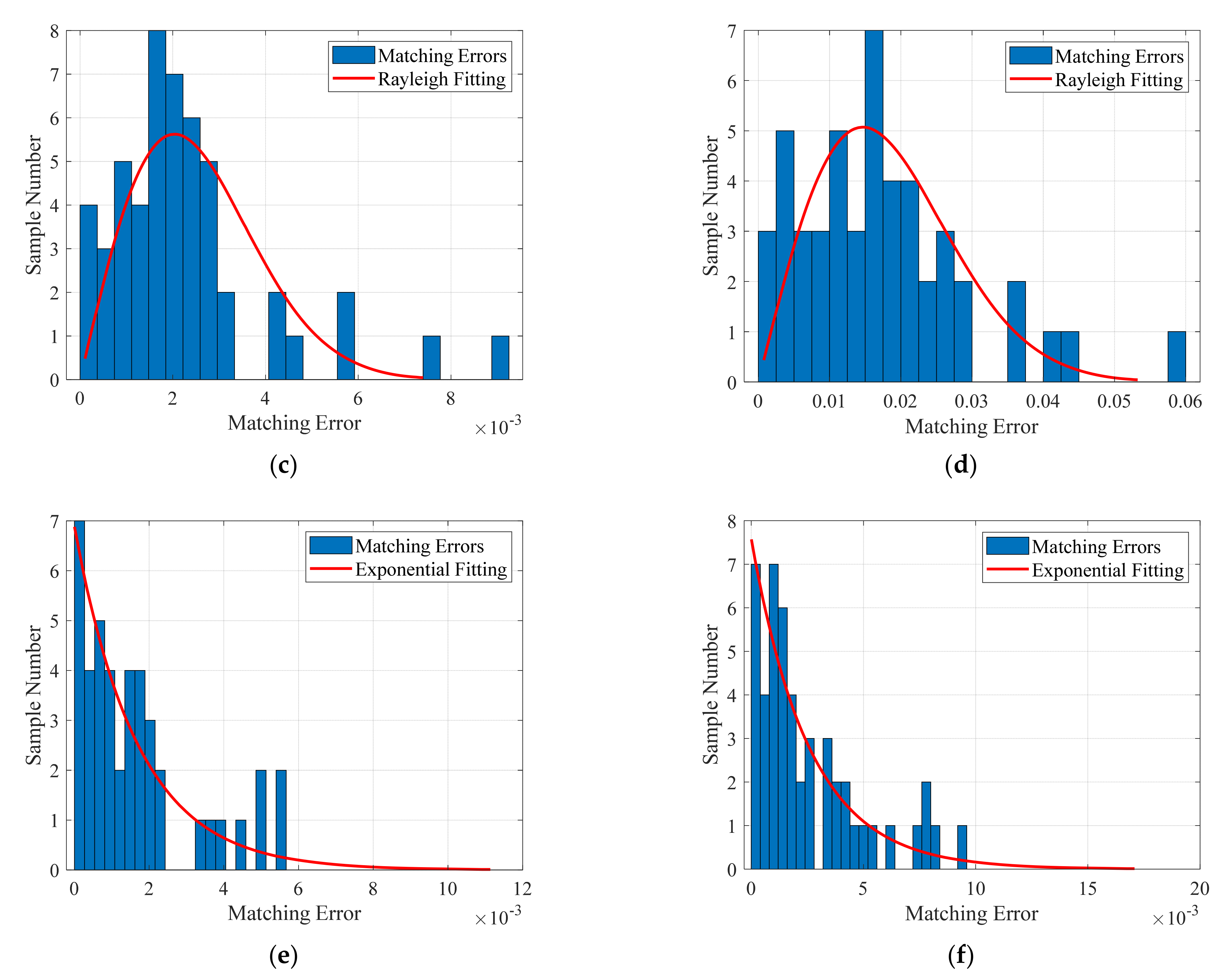
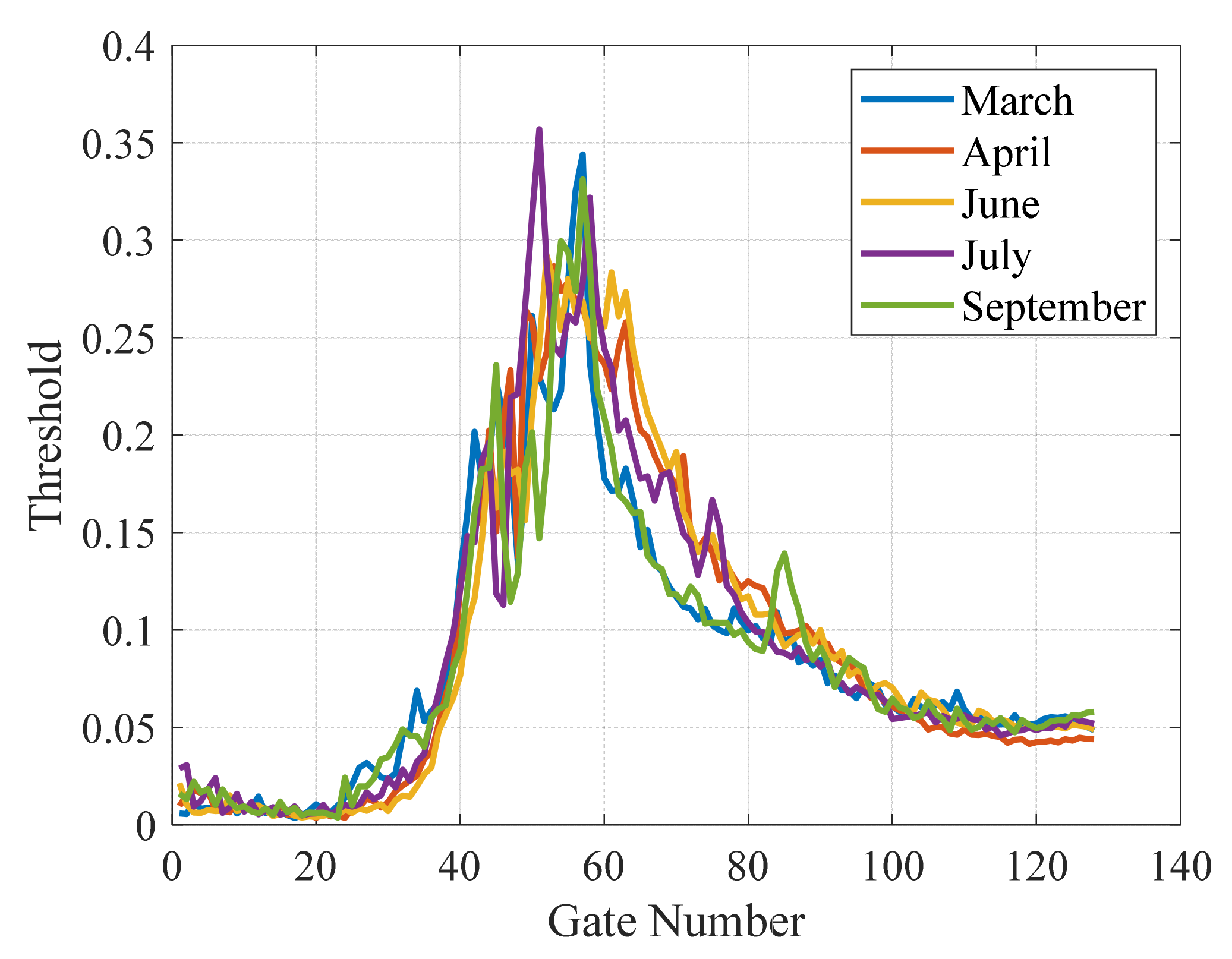
2.3. Adaptive Threshold Judgment Based on Error Distribution

In step 6, the matching errors corresponding to each waveform are obtained. These errors reflect the differences between the waveforms and the standard echo model at each gate. The larger the error, the greater the degree of contamination of the waveform at this gate, whereas the smaller the error, the lighter the degree of contamination of the waveform at this gate. The basic concept of waveform reconstruction is to use the partial waveform with less contamination to repair the partial waveform with more contamination. As the satellite flight distance corresponding to a group of waveforms is only approximately 35 km, the sea surface does not change dramatically at this spatial scale. Therefore, if a group of waveforms is not contaminated, their morphologies should be uniform and consistent. Thus, it is reasonable to use a group of waveforms as a unit and use the inside information to perform waveform reconstruction. Based on the above analysis, it can be concluded that, prior to waveform reconstruction, two tasks need to be completed: deciding on a method for dividing the waveforms into “reference waveforms for reconstruction” and “contaminated waveforms waiting for reconstruction”, and selecting the criteria that should be adopted after the division for reconstruction. This section examines the first task, that is, how to set an appropriate error threshold.

Step 7: Adaptive threshold judgment. As the amplitudes of the waveform at different gates vary in the range direction and the shapes of a group of waveforms are consistent in the azimuth direction, waveform reconstruction should be carried out based on each gate of a waveform unit. Figure 5a shows the matching error matrix corresponding to the coastal waveforms of experimental area 1 in March, and Figure 5b shows the median values of the matching errors at all gates for the different months. It can be seen that the magnitudes of the errors change at different gates, so it is not feasible to set a unified threshold to divide the waveforms. Instead, judgment thresholds should be generated adaptively based on the distribution characteristics of the errors.

To avoid the influence of individual maximum values on the error distribution, the outliers are first removed based on twice the median, while the error distribution at each gate is observed afterwards. Figure 5c–f exhibit two kinds of typical histograms of the errors, respectively. The error values in Figure 5c,d first have short increasing processes, and then gradually decrease, whereas the error values in Figure 5e,f only exhibit declining processes. According to the above changing characteristics, the two kinds of error histograms are fitted by Rayleigh and exponential distributions, respectively, and the results are shown as red curves in Figure 5c–f. It can be observed that the fitting degrees are all satisfactory.

The probability density function and the mean value calculation equation of the Rayleigh distribution can be expressed as:

$$f(x)=\frac{x}{{\sigma }^2}{e}^{-\frac{x^2}{2{\sigma }^2}},x>0;$$

(11)

$$E(x)=\sqrt{\frac{\pi }{2}}\sigma \approx 1.253\sigma ;$$

(12)

The probability density function and the mean value calculation equation of the exponential distribution can be expressed as:

$$f(x)=\lambda e^{-\lambda x},x>0;$$

(13)

$$E(x)=1/\lambda .$$

(14)

As the number of error samples is quite small, it is difficult to judge the distribution of errors in a timely manner. Therefore, to enhance the robustness of the method, the matching errors are simultaneously fitted by Rayleigh and exponential distributions, and the sum of the two mean values is taken as an adaptive threshold. When the error is less than the threshold, the corresponding waveform quality is judged as “Good” otherwise, it is judged as “Bad”. To guarantee that the original information (epoch and SWH) in the leading edge remains the same, the samples in [−2, 2] gates around the peak value (the corresponding wave crest contains the epoch obtained after step 5) are kept unchanged, even if they are judged as “Bad”. In the next step of waveform reconstruction, the “Good” waveform will be used to reconstruct the “Bad” waveform. Figure 6 shows the adaptive thresholds of experimental area 1. It can be observed that the judgment thresholds vary for different months and gates.

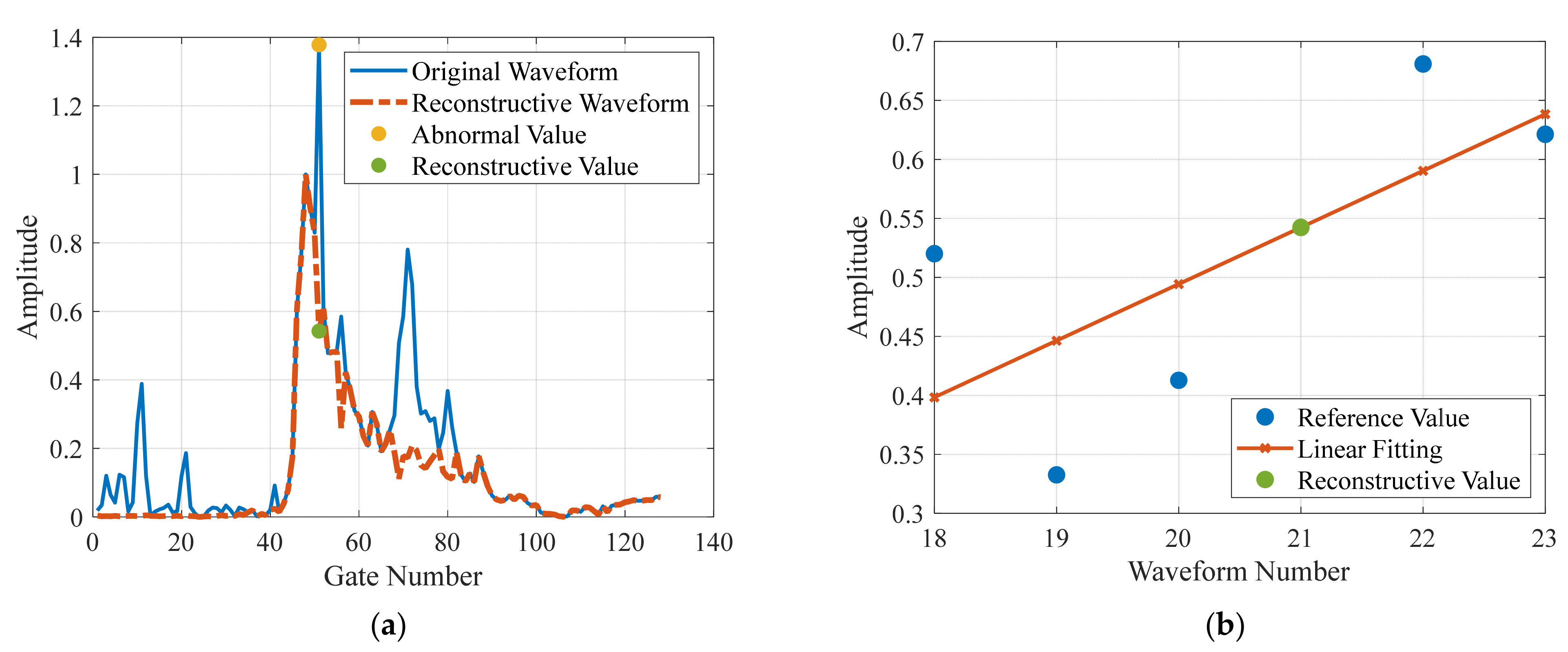
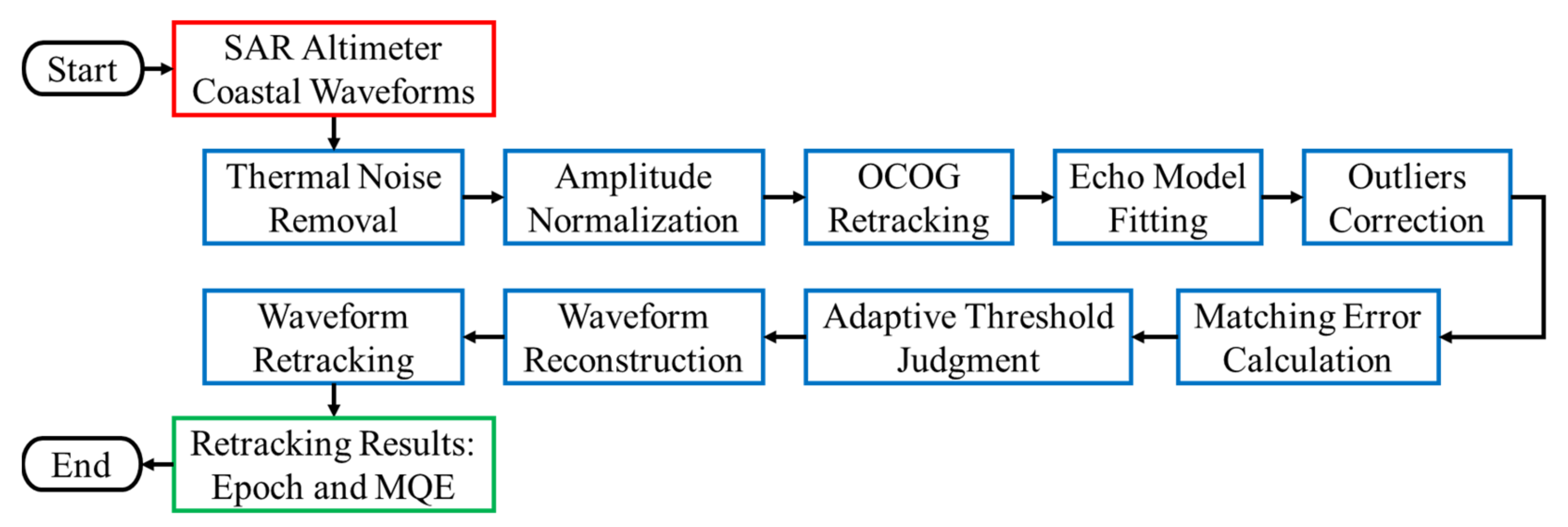
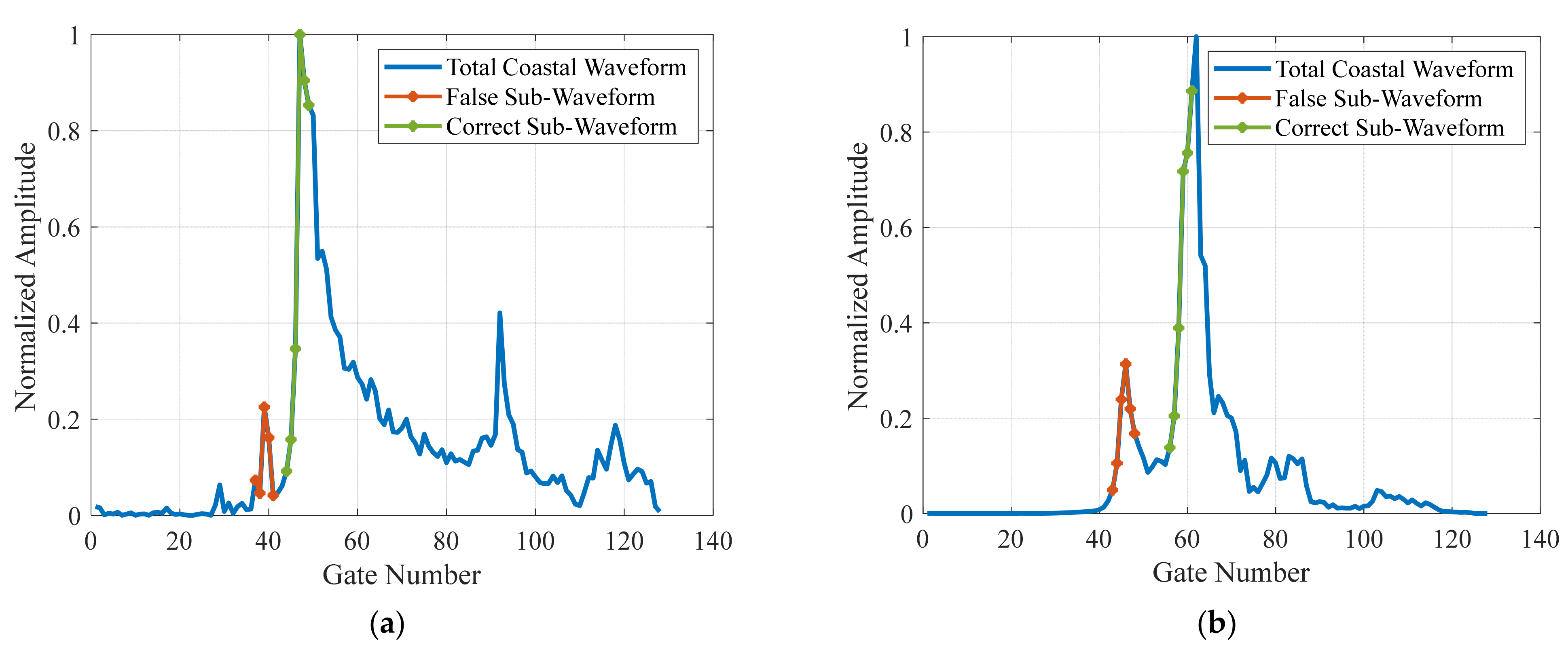
2.4. Waveform Reconstruction and Retracking Method

After processing in step 7, each gate of each waveform is attached to a quality flag (“Good” or “Bad”). In other words, for a certain gate position, we know which waveforms have good and bad quality. The previous analysis shows that the shapes of a group of waveforms are consistent; thus, the “Bad” waveforms can be reconstructed based on the nearest “Good” waveform by linear prediction. Finally, the waveforms can be retracked to obtain the retrieval results. The specific implementation steps are as follows:

Step 8: Nearest waveform reconstruction. Supposing that the gate k of a waveform is judged to be “Bad,” the five nearest waveforms with “Good” gate k are searched, and the value of the “Bad” gate k can be predicted through linear fitting. As shown in Figure 7a, gate 51 of the 21st waveform (blue curve) is judged to be “Bad” (yellow dot), and the nearest waveforms with “Good” gate 51 are numbered 18, 19, 20, 22, and 23, respectively. The amplitudes at gate 51 of the above original waveforms are taken as reference values (blue dots in Figure 7b) for linear fitting (red line in Figure 7b), and the reconstructive value of the 21st waveform at gate 51 can be predicted as the green dot in Figure 7b. After reconstructing all the “Bad” gates of the 21st waveform, the reconstructed result is shown by the red dotted line in Figure 7a. It can be seen that the contaminated partial waveform has been repaired, and the echo form is much closer to the standard ocean echo model.

Figure 8a,b show the reconstruction results corresponding to the waveforms in Figure 2b,d. It can be observed that the reconstructed waveforms are more uniform and regular, and the partial contamination in the noise and signal regions is successfully repaired.

Step 9: Waveform retracking. The retracking procedure is performed after waveform reconstruction based on the least-squares algorithm, and the epoch and MQE results can be obtained. To test the effect of the waveform reconstruction, the original waveforms are also retracked. In addition, most of the existing methods focus on extracting partial sub-waveforms from the contaminated waveform and using empirical algorithms to perform retracking. In this study, the NPPR algorithm is selected as a contrast method, which mainly considers the spike characteristics of the SAR waveform. The NPPR can be further divided into NPPOR and NPPTR according to whether the sub-waveform retracking adopts the OCOG algorithm or threshold algorithm.

The implementation principle of the NPPR algorithm is as follows in [30]. First, the starting and ending thresholds of the sub-waveform are calculated as:

$$T_{start}=\sqrt{\frac{(N-2)\cdot {\displaystyle \sum _{k=1}^{N-2}{(d_2^k)}^2-{({\displaystyle \sum _{k=1}^{N-2}{d}_2^k})}^2}}{(N-2)(N-3)}};$$

(15)

$$T_{end}=\sqrt{\frac{(N-1)\cdot {\displaystyle \sum _{k=1}^{N-1}{(d_1^k)}^2-{({\displaystyle \sum _{k=1}^{N-1}{d}_1^k})}^2}}{(N-1)(N-2)}}.$$

(16)

where $d_1^k$ and $d_2^k$ are the differences between adjacent and separated samplings of the waveform, respectively.

When $d_1^k$ is greater than $T_{start}$ or less than $T_{end}$, for the first time, the current gate is judged as the starting or ending position of the sub-waveform. Then, the sub-waveform is expanded forward and backward to ensure that the total sampling number is greater than five. The current sub-waveform is judged as the primary peak, only if its maximum value exceeds 1/3 of the maximum value of the total waveform, and the search continues backward until the condition is met. Finally, the sub-waveform is retracked using the threshold algorithm to obtain the epoch results.

The processing flow of the SAR altimeter coastal waveforms proposed in this study is illustrated in Figure 9.

3. Results

3.1. MQE Comparison and Retracking Results for Area 1

For all the original coastal waveforms, the NPPR algorithm is used to select the sub-waveforms. Figure 10a,b show two typical results, and the blue curves represent the total coastal waveforms. In Figure 10a, the red curve represents the sub-waveform selected for the first time. After comparing the peak value of the sub-waveform with that of the total waveform, it is believed that the current sub-waveform is not the primary peak. The search continued backwards, and the correct sub-waveform is extracted at the end, as shown by the green curve in Figure 10a. However, as the NPPR algorithm is only based on a simple numerical calculation and does not consider the actual physical meaning of the waveform, it cannot guarantee that the final extracted sub-waveform corresponds to the correct seawater peak. As shown in Figure 10b, the sub-waveform finally determined to be correct is located around gate 60, which is much larger than the nominal tracking point. This is because the power of this sub-waveform is very large, which weakens the peak that corresponds to seawater (the red curve in Figure 10b). From the analysis above, it can be concluded that the NPPR algorithm has certain limitations. Therefore, the results obtained from the threshold retracking of the sub-waveforms are bound to have errors.

The reconstructed coastal waveforms are retracked according to the least-squares algorithm, and the two typical results are shown in Figure 11. The blue curves represent the reconstructed coastal waveforms, and the red curves represent the final iteration results of the echo model. It can be seen that the quality of the coastal waveform in Figure 11a is worse than that in Figure 11b, but the matching degrees between the two waveforms and the final echo models are both good. This demonstrates that the shapes of the reconstructed coastal waveforms are consistent with the ocean echo model; therefore, the success rate of retracking will be greatly improved.

The MQE obtained by echo model fitting is recorded as MQE_1. The MQE obtained by retracking the reconstructed waveform is recorded as MQE_2. The MQE obtained by retracking the original waveform is recorded as MQE_3. As MQE reflects the difference between the coastal waveform and the echo model, the smaller the value, the closer the waveform is to the theoretical model; therefore, if MQE_2 is smaller than MQE_1, it is considered that the reconstruction processing improves the waveform quality. The MQE improvement proportions for each month in experimental area 1 are presented in the first row of

Table 2. MQE improvement proportions and retracking success rates for experimental area 1.

No. Month		1	2	3	4	5
MQE improvement proportion		91.86%	84.44%	84.88%	78.49%	91.86%
Retracking success rate	Without Reconstruction	37.21%	42.22%	51.16%	40.86%	38.37%
	With Reconstruction	90.70%	73.33%	76.58%	79.57%	87.21%
	Increasing Percentage	53.49%	31.11%	25.42%	38.71%	48.84%

. It can be seen that for the coastal waveform data of all five months, the proportions of quality improvement are higher than 78%.

To evaluate whether the waveform retracking is successful, an index needs to be set. It is known that the larger the MQE, the greater the deviation of the waveform from the theoretical model, and the more likely the retracking will fail. Therefore, the index can be set based on the MQE results. The MQE medians for each month of experimental area 1 are calculated, and the mean value of these medians is 0.0038. Set the double mean value of 0.008 as the threshold, and if the MQE after retracking is smaller than 0.008, retracking is considered successful. Thus, the success rate of retracking for the reconstructed waveforms and original waveforms can be calculated based on MQE_2 and MQE_3. The retracking success rates for each month in experimental area 1 are listed in the last three rows of Table 2. Among them, “Without Reconstruction” represents the results of the original waveforms, “With Reconstruction” represents the results of the reconstructed waveforms, and “Increasing Percentage” represents the differences between the above two results. It can be seen that the retracking success rates of the reconstructed waveforms are higher than 73%, with a maximum value of 90%. In the meantime, the success rates have been significantly improved, and the maximum “Increasing Percentage” is 53%.

Figure 12a shows the epoch-retracking results for experimental area 1 in August, and the results for the other months are similar. In the figure, the green dotted line represents the OCOG retracking result, the red dotted line represents the NPPTR result, the blue solid line represents the retracking result of the reconstructed waveform, and the yellow solid line represents the retracking result of the original waveform. The failing part of the retracking in the blue and yellow solid lines is replaced with the corresponding results of the model fitting. It can be observed that the epoch-retracking results of the reconstructed waveforms have an obviously improved regularity. While affected by waveform contamination, the retracking results of other algorithms have many burrs (such as the NPPTR and original waveform retracking results) or gradually deviate from the nominal tracking point of the altimeter (such as the OCOG retracking results).

After obtaining the epoch-retracking result, the SSH can be retrieved by combining the altimeter nominal tracking point $G_0$, satellite orbit height $H$, and the onboard tracking range word $R_0$. The calculation equation is as follows:

$$\mathrm{SSH}=H-(R_0-G_0+\mathrm{Epoch})$$

(17)

The SSH retrieval data of experimental area 1 over five months are averaged to obtain the final mean SSH data, and the results are shown in Figure 12b, in which the meaning of each curve is the same as that in Figure 12a. It can be seen that the SSH retrieval results of the reconstructed waveforms have good continuity, and the magnitude of change is about 2 m, which is consistent with the changing characteristics of real SSH. Although the OCOG results are continuous, the magnitude of the change reaches approximately 10 m. Such a large change is unlikely to occur within the altimeter observation range of 35 km. This is mainly because the estimation of the OCOG algorithm is based on the total waveform; therefore, partial contamination of the waveform has a considerable impact on the retracking results. There are many jump points in the results of NPPTR and a few in the results of the original waveform; thus, the SSH qualities are both unsatisfactory.

3.2. SSH Retrieval Results and Precision Validation of Area 2

The SAR altimeter coastal waveform data of experimental area 2 are processed according to the procedure shown in Figure 9, and the MQE results are evaluated using the same method as area 1. The MQE improvement proportions and retracking success rates for each pass in experimental area 2 are presented in

Table 3. MQE improvement proportions and retracking success rates for experimental area 2.

No. Pass	MQE Improvement Proportion	Retracking Success Rate
		without Reconstruction	with Reconstruction	Increasing Percentage
1	68.13%	21.98%	53.85%	31.87%
2	93.94 %	42.42%	97.98%	55.56%
3	63.64%	49.09%	61.82%	12.73%
4	92.06%	65.08%	93.65%	28.57%
5	59.14%	65.59%	69.89%	4.30%
6	83.00%	54.00%	91.00%	37.00%
7	63.00%	86.00%	88.00%	2.00%
8	79.59%	58.16%	96.94%	38.78%
9	88.33%	61.67%	86.67%	25.00%
10	91.23%	42.11%	87.72%	45.61%
11	84.09%	57.95%	94.32%	36.37%
12	82.83 %	58.59%	92.93%	34.34%
13	94.95%	47.47%	97.98%	50.51%
Mean	80.30%	54.62%	85.60%	30.98%

, and the mean values for the whole year are shown in the last row. It can be seen that for the coastal waveform data of 2022, the mean proportion of quality improvement is 80.30%. The mean retracking success rates of the original and reconstructed waveforms are 54.62% and 85.60%, respectively, and the mean increasing percentage is 30.98%.

Figure 13a,b present the epoch-retracking results of experimental area 2 in March and August, and the results for the other months are analogous. Similar to the results of area 1, the epoch-retracking results of the reconstructed waveforms show obviously improved regularity. While affected by waveform contamination, the retracking results of other algorithms are not satisfactory.

According to Equation (15), the SSH retrieval data for experimental area 2 for a whole year are obtained and averaged to gain the final SSH data, and the results are shown in Figure 14, in which the meaning of each curve is the same as that in Figure 13. It can be seen that the SSH retrieval results of the reconstructed waveforms have good performance and a fluctuation degree that is smaller than that of the original waveforms. While the magnitude of the change in OCOG retrieval results is relatively large, there are many jumps in the results of NPPTR.

The noise levels of the SSH data retrieved by different methods are calculated based on the along-track odd-even differential approach [44], and the results are presented in the first row of

Table 4. Noise level and RMSE results of the SSH data retrieved by different methods.

Method	OCOG	NPPTR	without Reconstruction	with Reconstruction
Noise level	26.23 cm	27.53 cm	12.75 cm	6.32 cm
RMSE	59.87 cm	39.82 cm	15.24 cm	7.06 cm

. Among them, “OCOG “ and “NPPTR” indicate that the SSH data are obtained by OCOG retracking and NPPTR, respectively, and “Without Reconstruction” and “With Reconstruction” mean that the SSH data are obtained by original and reconstructed waveform retracking, respectively. It can be noticed that the noise levels of the OCOG and NPPTR results are relatively high. The main reason is that the accuracies of the empirical retracking methods are relatively low because these methods have no physical significance that can be used as a reference, and the retracking result will contain large errors if the waveform is contaminated. As the method of model retracking is adopted, the noise level results of “Without Reconstruction” and “With Reconstruction” are significantly decreased. Among them, the retracking results of the original waveform without reconstruction are basically consistent with the Sentinel-3B GDR public results, and the failing part of the retracking has been replaced with the corresponding results of model fitting to be comparable with the reconstructive results.

The retrieved SSH data are further verified by comparing them to the MSS model data along the satellite pass. Here the MSS2018 model from the Technical University of Denmark (DTU) is used, which is averaged over years of SSH measurements by satellite altimeters, so it can reflect the changes in SSH to a certain extent. As the coastal area is confined in space and the observation time is only 5 s, the multiple corrections of altimeter height measurement, such as systematic internal delay, ionospheric and tropospheric delay, ocean tides, etc., can be considered a bias. The grid resolution of the MSS model is only 1 min, which is much coarser than the sample distance of the 20 Hz waveform; thus, the MSS data are interpolated first and then extracted according to the information of latitudes and longitudes from GDR products. The comparison results are shown in Figure 15, where the yellow and blue lines represent the retrieved SSH data of the original and reconstructed waveforms, respectively, and the purple line represents the extracted MSS data. Note that the bias between MSS and SSH has been removed. The changing characteristic of the blue line coincides well with the purple line, which indicates that the SSH data of reconstructed waveforms matches well with the MSS data. The fluctuation degree of the yellow line is greater than that of the blue line, which implies that the SSH data of the original waveforms deviates more from the MSS data. By taking the MSS data as a reference value, the root-mean-square errors (RMSE) are calculated, and the results of different methods are shown in the second row of Table 4.

In Table 4, the RMSE results of the original and reconstructed waveforms are 15.24 cm and 7.06 cm, respectively, which are in good agreement with the estimation results of the noise level, and the slightly larger values are probably affected by the sea level anomaly and ocean tides. The noise level estimation results represent the 20 Hz SSH precisions; therefore, it is validated that the partial reconstruction method for SAR altimeter coastal waveforms proposed in this study has successfully improved the SSH measurement precision by a factor of two, and the corresponding 1 Hz SSH precisions of the original and reconstructed waveforms are 2.85 cm and 1.41 cm, respectively.

4. Conclusions

Satellite radar altimeters have been successfully used for decades to monitor global-scale ocean circulation and provide high-precision open-ocean SSH data for many disciplines. However, the precision of the SSH measurement results in coastal areas is poor because of the impact of land contamination and human activities. For traditional altimeters, some retracking methods have been proposed based on the echo model, which improves the SSH retrieval precision of coastal waveforms to a certain extent. The along-track high-resolution waveform characteristics of the new SAR altimeter require different treatments. This study proposes an innovative processing method for SAR altimeter coastal waveforms that can improve the success rate of retracking and the retrieval precision of SSH significantly.

In the proposed method, the coastal waveforms are first fitted through sliding based on the high-precision SAR altimeter echo model, and the preliminary epoch estimation results are provided with the help of outlier correction. Then, by calculating the matching errors between the coastal waveform and the echo model and generating adaptive thresholds based on the distribution characteristics of errors, the partial reference waveforms with good quality and the partially contaminated waveforms with poor quality are classified. Finally, the contaminated waveforms are reconstructed through the nearest linear fitting, and the abnormal sampling values in the noise and signal regions are successfully repaired.

The data used in this study were obtained from the L2 GDR products of satellite Sentinel-3B, and the SAR waveforms were extracted as the processing object. The two experimental areas are located on the nearshores of the South China Sea and the West Korean Gulf. By calculating the MQE between the waveform and model, it is proved that for the coastal data of experimental area 1, the proportion of waveform quality improvement brought by partial reconstruction is greater than 78%, the maximum success rate of retracking is 90%, and the maximum improvement percentage is 53%. For a year of coastal data in experimental area 2, the mean proportion of waveform quality improvement is 80.30%, the mean retracking success rate of the reconstructed waveforms is 85.60%, and the mean increasing percentage is 30.98%.

To further evaluate the effectiveness of the proposed method, the noise levels of the area 2 SSH data retrieved by different methods are calculated based on the along-track odd-even differential approach. The 20 Hz SSH precisions of the original and reconstructed coastal waveforms are 12.75 cm and 6.32 cm, respectively, and the corresponding 1 Hz precisions are 2.85 cm and 1.41 cm, respectively. Therefore, it is validated that the proposed partial reconstruction method for SAR altimeter coastal waveforms has successfully improved the SSH measurement precision by a factor of two.

References

1. Bannoura, W.J.; Wade, A.; Srinivas, D.N. NOAA ocean surface topography mission Jason-2 project overview. In Proceedings of the OCEANS 2005 MTS/IEEE, Washington, DC, USA, 17–23 September 2005; pp. 2155–2159. [Google Scholar]
2. Phalippou, L.; Enjolras, V. Re-tracking of SAR altimeter ocean power-waveforms and related accuracies of the retrieved sea surface height, significant wave height and wind speed. In Proceedings of the 2007 IEEE International Geoscience and Remote Sensing Symposium (IGARSS), Barcelona, Spain, 23–28 July 2007; pp. 3533–3536. [Google Scholar]
3. Tournadre, J.; Chaprono, B. Altimeter as an imager of the sea surface roughness: Comparison of SAR and LRM modes. In Proceedings of the 2020 IEEE International Geoscience and Remote Sensing Symposium (IGARSS), Waikoloa, HI, USA, 26 September–2 October 2020; pp. 3541–3544. [Google Scholar]
4. Jiang, M.; Xu, K.; Xu, X.; Shi, L.; Yu, X.; Liu, P. 2019: Range noise level estimation of the HY-2B radar altimeter and its comparison with Jason-2 and Jason-3 altimeters. In Proceedings of the 2019 IEEE International Geoscience and Remote Sensing Symposium (IGARSS), Yokohama, Japan, 28 July–2 August 2019; pp. 8312–8315. [Google Scholar]
5. Dinardo, S.; Lucas, B.; Benveniste, J. Sentinel-3 STM SAR ocean retracking algorithm and SAMOSA model. In Proceedings of the 2015 IEEE International Geoscience and Remote Sensing Symposium (IGARSS), Milan, Italy, 26–31 July 2015; pp. 5320–5323. [Google Scholar]
6. Donlon, C.J.; Cullen, R.; Giulicchi, L.; Vuilleumier, P.; Francis, C.R.; Kuschnerus, M.; Simpson, W.; Bouridah, A.; Caleno, M.; Bertoni, R.; et al. The Copernicus Sentinel-6 mission: Enhanced continuity of satellite sea level measurements from space. Remote Sens. Environ. 2021, 258, 112395. [Google Scholar] [CrossRef]
7. Yang, J.; Zhang, J.; Wang, C. Sentinel-3A SRAL global statistical assessment and cross-calibration with Jason-3. Remote Sens. 2019, 11, 1573. [Google Scholar] [CrossRef] [Green Version]
8. Donlon, C.; Cullen, R.; Giulicchi, L.; Fornari, M.; Vuilleumier, P. Copernicus Sentinel-6 Michael Freilich satellite mission: Overview and preliminary in orbit results. In Proceedings of the 2021 IEEE International Geoscience and Remote Sensing Symposium (IGARSS), Brussels, Belgium, 11–16 July 2021; pp. 7732–7735. [Google Scholar]
9. Hithin, N.K.; Remya, P.G.; Nair, T.M.B.; Harikumar, R.; Kumar, R.; Nayak, S. Validation and Intercomparison of SARAL/AltiKa and PISTACH-Derived Coastal Wave Heights Using In-Situ Measurements. IEEE J. Sel. Top. Appl. Earth Obs. Remote Sens. 2015, 8, 4120–4129. [Google Scholar] [CrossRef]
10. Gower, J.F.R. Intercalibration of wave and wind data from TOPEX/POSEIDON and moored buoys off the west coast of Canada. J. Geophys. Res. 1996, 101, 3817–3829. [Google Scholar] [CrossRef]
11. Dinardo, S.; Fenoglio-Marc, L.; Buchhaupt, C.; Becker, M.; Scharroo, R.; Fernandes, M.J.; Benveniste, J. Coastal SAR and PLRM altimetry in German Bight and West Baltic Sea. Adv. Space Res. 2018, 62, 1371–1404. [Google Scholar] [CrossRef]
12. Brown, G. The average impulse response of a rough surface and its applications. IEEE Trans. Antennas Propag. 1977, 25, 67–74. [Google Scholar] [CrossRef]
13. Raney, R.K. The delay/Doppler radar altimeter. IEEE Trans. Geosci. Remote Sens. 1998, 36, 1578–1588. [Google Scholar] [CrossRef]
14. Egbert, G.D.; Bennett, A.F.; Foreman, M.G.G. TOPEX/POSEIDON tides estimated using a global inverse model. J. Geophys. Res. 1994, 99, 24821–24852. [Google Scholar] [CrossRef] [Green Version]
15. Liu, X.; Cui, X.; Dong, W.; Sun, H.; Lu, Y. Simulation of wet atmospheric delay correction for interferometric imaging altimeter based on radiometer. In Proceedings of the IET International Radar Conference 2020 (IET IRC 2020), Online, 4–6 November 2020; pp. 511–516. [Google Scholar]
16. Fernandes, M.J.; Pires, N.; Lazáro, C.; Nunes, A. L Tropospheric delays from GNSS for application in coastal altimetry. Adv. Space Res. 2013, 51, 1352–1368. [Google Scholar] [CrossRef]
17. Lebedev, S.; Sirota, A.; Medvedev, D.; Khlebnikova, S.; Vignudelli, S.; Snaith, H.M.; Cipollini, P.; Venuti, F.; Lyard, F.; Bouffard, J.; et al. Exploiting satellite altimetry in coastal ocean through the ALTICORE project. Russ. J. Earth Sci. 2008, 10, ES1002. [Google Scholar] [CrossRef] [Green Version]
18. Coastal and Hydrology Altimetry Product (PISTACH) Handbook; CLS-DOS-NT-10–246, SALP-MU-P-OP-16031-CN01/00; National Center of Spatial Studies: Paris, France, 2010.
19. Ray, C.; Martin-Puig, C.; Clarizia, M.P.; Ruffini, G.; Dinardo, S.; Gommenginger, C.; Benveniste, J. SAR altimeter backscattered waveform model. IEEE Trans. Geosci. Remote Sens. 2015, 53, 911–919. [Google Scholar] [CrossRef]
20. Martin, T.V.; Zwally, H.J.; Brenner, A.C.; Bindschadler, R.A. Analysis and retracking of continental ice sheet radar altimeter waveforms. J. Geophys. Res. 1983, 88, 1608–1616. [Google Scholar] [CrossRef]
21. Legresy, B.; Remy, F. Surface characteristics of the Antarctic ice sheet and altimetric observations. J. Glaciol. 1997, 43, 197–206. [Google Scholar] [CrossRef] [Green Version]
22. Wingham, D.J.; Rapley, C.G.; Griffiths, H. New techniques in satellite altimeter tracking system. In Proceedings of the 1986 IEEE International Geoscience and Remote Sensing Symposium (IGARSS), Zurich, Switzerland, 8–11 September 1986; pp. 1339–1344. [Google Scholar]
23. Davis, C.H. A robust threshold retracking algorithm for measuring ice-sheet surface elevation change from satellite radar altimeter. IEEE Trans. Geosci. Remote Sens. 1997, 35, 974–979. [Google Scholar] [CrossRef]
24. Dabo-Niang, S.; Ferraty, F.; Vieu, P. On the using of modal curves for radar waveforms classification. Comput. Statist. Data. Anal. 2007, 51, 4878–4890. [Google Scholar] [CrossRef]
25. Yang, L. Study on Satellite Radar Altimeter Retrieval Algorithms over Coastal Seas and under High Sea State Events. Ph.D. Thesis, Nanjing University of Science & Technology, Nanjing, China, 2009. [Google Scholar]
26. Ganguly, D.; Chander, S.; Desai, S.; Chauhan, P. A Subwaveform-Based Retracker for Multipeak Waveforms: A Case Study over Ukai Dam/Reservoir. Mar. Geod. 2015, 38, 581–596. [Google Scholar] [CrossRef]
27. Passaro, M.; Cipollini, P.; Vignudelli, S.; Quartly, G.D.; Snaith, H.M. ALES: A multi-mission adaptive subwaveform retracker for coastal and open ocean altimetry. Remote Sens. Environ. 2014, 145, 173–189. [Google Scholar] [CrossRef] [Green Version]
28. Passaro, M.; Rose, S.; Andersen, O.; Boergens, E.; Calafat, F.; Dettmering, D.; Benveniste, J. ALES+: Adapting a homogenous ocean retracker for satellite altimetry to sea ice leads, coastal and inland waters. Remote Sens. Environ. 2018, 211, 456–471. [Google Scholar] [CrossRef] [Green Version]
29. Passaro, M.; Rautiainen, L.; Dettmering, D.; Restano, M.; Hart-Davis, M.G.; Schlembach, F.; Särkkä, J.; Müller, F.L.; Schwatke, C.; Benveniste, J. Validation of an empirical subwaveform retracking strategy for SAR altimetry. Remote Sens. 2022, 14, 4122. [Google Scholar] [CrossRef]
30. Jain, M.; Andersen, O.B.; Dall, J.; Stenseng, L. Sea surface height determination in the Arctic using Cryosat-2 SAR data from primary peak empirical retrackers. Adv. Space Res. 2015, 55, 40–50. [Google Scholar] [CrossRef]
31. The European Space Agency. Available online: https://www.esa.int/ (accessed on 10 January 2023).
32. Aviso+ Satellite Altimetry Data. Available online: https://www.aviso.altimetry.fr/en/home.html (accessed on 10 January 2023).
33. EUMETSAT Data Store. Available online: https://data.eumetsat.int/extended?query=SRAL%20Level%202%20Altimetry%20Global%20-%20Sentinel-3# (accessed on 10 January 2023).
34. Guccione, P. Beam sharpening of Delay/Doppler altimeter data through chirp Zeta transform. IEEE Trans. Geosci. Remote Sens. 2008, 46, 2517–2526. [Google Scholar] [CrossRef]
35. Scagliola, M.; Guccione, P.; Giudici, D. Fully focused SAR processing for radar altimeter: A frequency domain approach. In Proceedings of the 2018 IEEE International Geoscience and Remote Sensing Symposium (IGARSS), Valencia, Spain, 22–27 July 2018; pp. 6699–6702. [Google Scholar]
36. Wingham, D.J.; Phalippou, L.; Mavrocordatos, C.; Wallis, D. The mean echo and echo cross product from a beamforming interferometric altimeter and their application to elevation measurement. IEEE Trans. Geosci. Remote Sens. 2004, 42, 2305–2323. [Google Scholar] [CrossRef]
37. Egido, A.; Smith, W.H.F. Fully focused SAR altimetry: Theory and applications. IEEE Trans. Geosci. Remote Sens. 2017, 55, 392–406. [Google Scholar] [CrossRef]
38. Wingham, D.J.; Giles, K.A.; Galin, N.; Cullen, R.; Armitage, T.W.; Smith, W.H. A semianalytical model of the synthetic aperture, interferometric radar altimeter mean echo, and echo cross-product and its statistical fluctuations. IEEE Trans. Geosci. Remote Sens. 2018, 56, 2539–2553. [Google Scholar] [CrossRef]
39. Scagliola, M.; Guccione, P. Datation and range calibration of radar altimeter exploiting fully focused SAR processing. IEEE Geosci. Remote Sens. Lett. 2021, 18, 480–483. [Google Scholar] [CrossRef]
40. Liu, X.; Kong, W.; Sun, H.; Lu, Y. Performance analysis of Ku/Ka dual-band SAR altimeter from an airborne experiment over South China Sea. Remote Sens. 2022, 14, 2362. [Google Scholar] [CrossRef]
41. Garcia, E.S.; Sandwell, D.T.; Smith, W.H.F. Retracking CryoSat-2, Envisat and Jason-1 radar altimetry waveforms for improved gravity field recovery. Geophys. J. Int. 2013, 196, 1402–1422. [Google Scholar] [CrossRef] [Green Version]
42. Halimi, A.; Mailhes, C.; Tourneret, J.; Thibaut, P.; Boy, F. A semi-analytical model for Delay/Doppler altimetry and its estimation algorithm. IEEE Trans. Geosci. Remote Sens. 2014, 52, 4248–4258. [Google Scholar] [CrossRef] [Green Version]
43. Taburet, N.; Zawadzki, L.; Vayre, M.; Blumstein, D.; Le Gac, S.; Boy, F.; Raynal, M.; Labroue, S.; Crétaux, J.-F.; Femenias, P. S3MPC: Improvement on Inland Water Tracking and Water Level Monitoring from the OLTC Onboard Sentinel-3 Altimeters. Remote Sens. 2020, 12, 3055. [Google Scholar] [CrossRef]
44. Liu, X.; Kong, W.; Sun, H.; Xu, Y.; Lu, Y. An improved altimeter in-orbit range noise-level estimation approach based on along-track differential method. Remote Sens. 2022, 14, 6250. [Google Scholar] [CrossRef]
Figure 1. (a) The locations of the two experimental areas used for coastal waveform processing and the corresponding subsatellite tracks. (b) The offshore distances of the subsatellite points in the two experimental areas. (c,d) The coastal details of experimental areas 1 and 2.
Remotesensing 15 01717 g001
Figure 2. Normalized coastal waveforms of experimental area 1 in (a) June and (b) September. Normalized coastal waveforms of experimental area 2 in (c) May and (d) September.
Remotesensing 15 01717 g002
Figure 3. Some typical coastal waveforms in the experimental area, with (a) single-peak (b) double-peak (c) multi-peak (d) slight contamination and (e,f) heavy contamination.
Remotesensing 15 01717 g003
Figure 4. (a) The epoch sequences obtained by processing the coastal waveforms of experiment area 1 in April after steps 3 (blue curve), 4 (red curve), and 5 (green curve). (b) The coastal waveforms before and after step 5 (dark and light blue curves), and the corresponding fitting models (red and green curves).
Remotesensing 15 01717 g004
Figure 5. (a) The matching error matrix corresponding to the coastal waveforms of experimental area 1 in March. (b) The median errors at all gates in different months for experimental area 1. (c,d) Two typical error histograms fit by the Rayleigh distribution. (e,f) Two typical error histograms fit by exponential distribution.
Remotesensing 15 01717 g005aRemotesensing 15 01717 g005b
Figure 6. Adaptive thresholds of experimental area 1 for different months and different gates.
Remotesensing 15 01717 g006
Figure 7. (a) The original contaminated coastal waveform (blue curve) and the corresponding reconstructive result (red dotted line). (b) The reference values (blue dots) used for linear fitting (red line) and the corresponding reconstructive value (green dot).
Remotesensing 15 01717 g007
Figure 8. The reconstruction results corresponding to the waveforms in Figure 2b (a) and Figure 2d (b).
Remotesensing 15 01717 g008
Figure 9. Processing flow of the SAR altimeter coastal waveforms.
Remotesensing 15 01717 g009
Figure 10. Two typical results of the NPPR algorithm in sub-waveform extraction (a,b). The blue curves represent the total coastal waveforms, the red curves represent the sub-waveforms determined to be false, and the green curves represent the sub-waveforms determined to be correct.
Remotesensing 15 01717 g010
Figure 11. Two typical retracking results of the reconstructed coastal waveforms (a,b). The blue curves represent the reconstructed coastal waveforms, and the red curves represent the final iteration results of the echo model.
Remotesensing 15 01717 g011
Figure 12. (a) Epoch-retracking results for experimental area 1 in September. (b) Mean SSH data for experimental area 1. The green and red dotted lines represent the OCOG retracking results and the NPPTR results, and the blue and yellow solid lines represent the retracking results of the reconstructed and original waveforms.
Remotesensing 15 01717 g012
Figure 13. Epoch-retracking results for experimental area 2 in (a) March and (b) August. The green and red dotted lines represent the OCOG retracking results and the NPPTR results, and the blue and yellow solid lines represent the retracking results of the reconstructed and original waveforms.
Remotesensing 15 01717 g013
Figure 14. Retrieved SSH data for experimental area 2 of year 2022.
Remotesensing 15 01717 g014
Figure 15. Validation of retrieved SSH data using the MSS model. The yellow and blue lines represent the SSH retrieval results of the original and reconstructed waveforms, and the purple line represents the MSS model.
Remotesensing 15 01717 g015