Article

Tropical Dry Forest Dynamics Explained by Topographic and Anthropogenic Factors: A Case Study in Mexico

1
Centro de Investigaciones en Geografía Ambiental, Universidad Nacional Autónoma de México, Morelia 58190, Mexico
2
Graduate School of Environmental Earth Science, Hokkaido University, Sapporo 060-0810, Japan
3
Posgrado en Geografía, Centro de Investigaciones en Geografía Ambiental, Universidad Nacional Autónoma de México, Morelia 58190, Mexico
4
Center for Biodiversity and Climate Change, Forestry and Forest Products Research Institute, Tsukuba 305-8687, Japan
*
Author to whom correspondence should be addressed.
Remote Sens. 2023, 15(5), 1471; https://doi.org/10.3390/rs15051471
Submission received: 31 December 2022 / Revised: 24 February 2023 / Accepted: 4 March 2023 / Published: 6 March 2023

Abstract

:
Tropical dry forest is one of the most threatened ecosystems, and it is disappearing at an alarming rate. Shifting cultivation is commonly cited as a driver of tropical dry forest loss, although it helps to maintain the forest coverage but with less density. We investigated tropical dry forest dynamics and their contributing factors to find out if there is an equilibrium between these two processes. We classified multi-temporal Sentinel-2A images with machine learning algorithms and used a logistic regression model to associate topographic, anthropogenic, and land tenure variables as plausible factors in the dynamics. We carried out an accuracy assessment of the detected changes in loss and gain considering the imbalance in area proportion between the change classes and the persistence classes. We estimated a 1.4% annual loss rate and a 0.7% annual gain rate in tropical dry forest and found that the topographic variable of slope and the anthropogenic variable of distance to roads helped explain the occurrence probability of both tropical forest loss and tropical forest gain. Since the area estimation yielded a wide confidence interval for both tropical forest loss and gain despite the measures that we took to counterbalance the disproportion in areas, we cannot conclude that the loss process was more intense than the gain process, but rather that there was an equilibrium in tropical dry forest dynamics under the influence of shifting cultivation.

1. Introduction

Tropical and subtropical dry forests are one of fourteen biomes identified at the global scale [1]. In Mexico, tropical dry forests (TDFs) cover extensive areas in the western Pacific lowland from southern Sonora to northern and central Chiapas [2]. TDFs host a large variety of fauna and flora, playing an important role in biodiversity conservation and providing food and shelter for local people [3,4]. Despite having the highest level of endemism in the American continent [5], TDFs in Mexico are conventionally perceived as having less commercial value compared with temperate forests, and they are mainly designated for shifting cultivation and cattle ranching [6,7].
Land use and land cover change (LULCC) contributes to about one-tenth of the annual carbon emissions [8], in which deforestation shares more than three times that of the other LULCC categories combined [9]. In Mexico, at the national level, TDF decreased at a rate of 0.4%, about 100,000 ha every year [10]. Regional studies have reported higher deforestation rates, reaching 1.4% per year [11]. Large dry forest tracts have disappeared in recent years mainly to support agriculture and cattle ranching. About 70% of pre-Hispanic TDF has been converted to other land use types, and about 62% of the remaining TDF is in an altered and disturbed state [6]. In addition to carbon loss, the loss of TDF leads to the loss of biodiversity and soil erosion and increases the vulnerability of local people who depend on TDFs for food and shelter. The disturbance also fundamentally alters environmental conditions and constrains the forest’s capacity to regenerate [12].
In previous studies, different drivers have been associated with the LULCC of tropical forests, such as the expansion of agriculture (frequently large-scale and industrialized) or livestock activities, as well as socio-economic conditions such as poverty. Especially, topographical and distance-related measures have been reported as determinant factors to explain which areas will undergo a LULCC process. For example, it was reported that the probability of an area experiencing a LULCC process is related to a poverty index, the population size of nearby settlements, topographical variables, and distance to roads [13]. Nonetheless, these can sometimes be a product of complex relationships [13,14].
Shifting cultivation is widely practiced in the global south and plays an important role in food security in Asian, African, and Latin American countries [15,16]. In Mexico, shifting cultivation is the main driver of disturbances in TDFs, especially in the southern part of the country [17]. This agriculture system includes cycles of clearing, cultivation, and fallow period. During clearing, the standing vegetation is cut down and burned to create fields and produce ash which provides nutrients for farming. The cleared parcels have an average size of 2.5 ha and crops are grown for subsistence [18]. Cultivation starts during the rainy season when maize crops are planted and harvested after six months of growth. After harvesting until the next plantation, livestock graze on crop residues. The cultivation cycle repeats for about 2–3 years and then the land is left to rest in a fallow period for about 3–8 or more years, during which natural vegetation grows as a mixture of shrubs and trees. Shifting cultivation creates a landscape with a mosaic of patches currently being cropped and patches in the fallow period with natural vegetation under various stages of regeneration. The regenerated natural vegetation keeps the area a forest, however, with less biomass density [19].
This paper aims to understand the contributing factors to the dynamics of TDFs and whether there is a balance between TDF loss and gain under the influence of shifting cultivation. We first obtained areas of TDF loss and gain by comparing multiple dates of land use land cover maps created by classifying Sentinel-2A images with a machine learning algorithm. Then, using a logistic regression model, we analyzed the plausible factors including topographic, anthropogenic, and land ownership that are associated with TDF changes. Lastly, we projected the areas of future TDF loss and gain to shifting cultivation.

2. Materials and Methods

2.1. Study Area

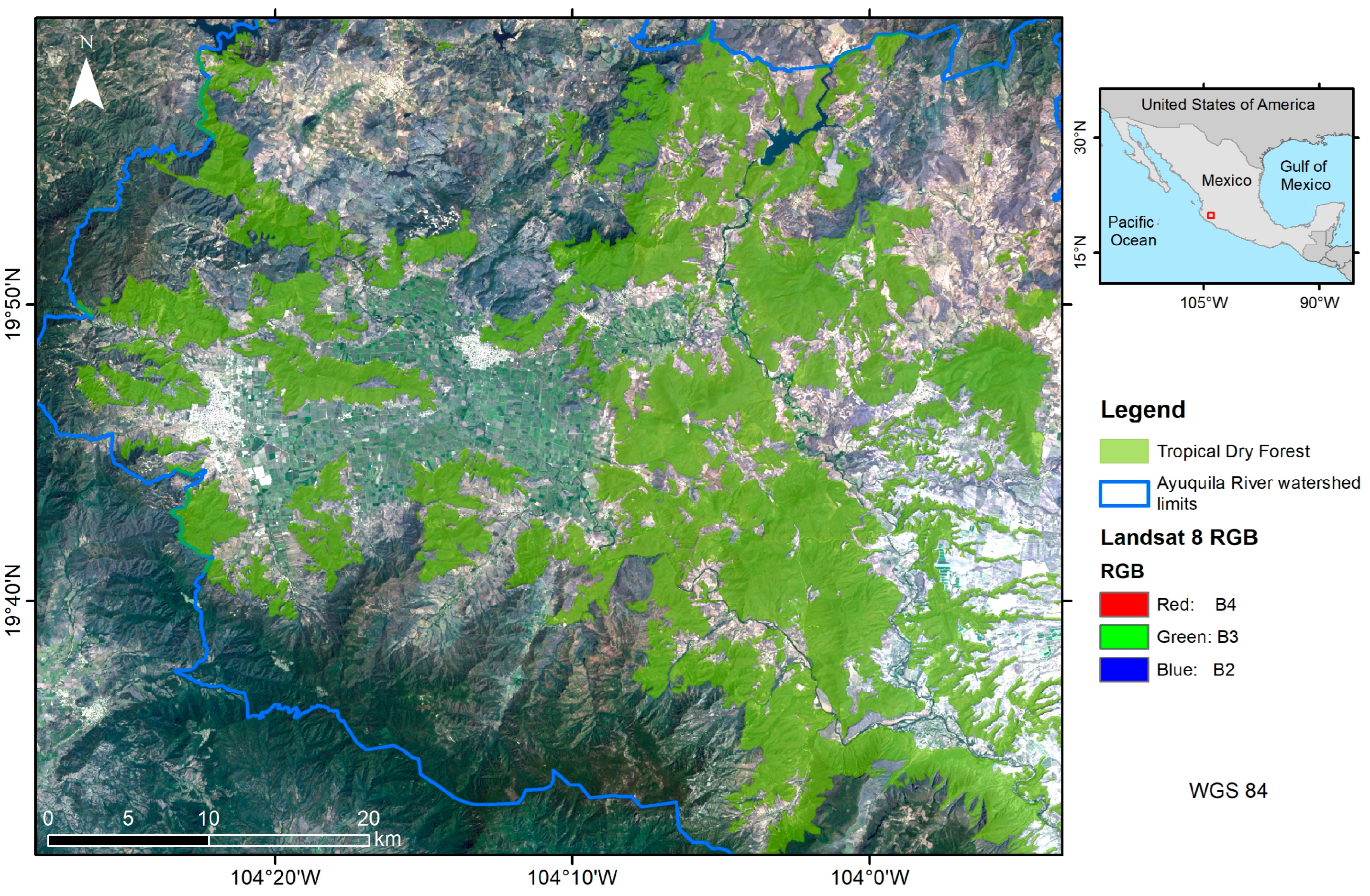
The study area is within the Ayuquila River watershed, in the state of Jalisco, Mexico (Figure 1). It is one of the first areas in Mexico designated as a Reduction of Emission from Deforestation and Forest Degradation (REDD+) experimental area because of its importance in biodiversity and water provision, among other ecosystem services [20]. The watershed has a wide range in topography, from 260 m to 2500 m above mean sea level (amsl). The monthly average temperature is about 18–22 degrees Celsius, and the annual average precipitation is 800–1200 mm, which occurs mainly during the rainy season, from June to October [21]. The dominant forest type is TDF, which is comprised of deciduous and semi-deciduous trees that lose their leaves during the dry season, typically from November to May. TDF covers about 24% of the watershed, and it has been intensively used for shifting cultivation, cattle grazing, and fuel wood collection. As in the rest of Mexico, most of the forests (59% to 80%) in the Ayuquila watershed are under the authority of ejidos, which is a communally managed land tenure system of rural agrarian settlements [18].

2.2. Data

This study collected and used a variety of datasets (Table 1). Sentinel-2A images were obtained from Google Earth Engine archive. All Sentinel-2A bottom-of-atmosphere reflectance images were atmospherically corrected with Copernicus scihub using the sen2cor algorithm. In addition, elevation data (Digital Elevation Model: DEM) were obtained from the official website of the National Institute of Statistics and Geography (INEGI) of Mexico with a 15 m spatial resolution, and the topographic variables of slope and aspect were calculated using the DEM to reflect terrain changes. Data on accessibility including distance to roads and distance to agriculture were calculated using the proximity function with roads data downloaded from the INEGI and agriculture data (including both irrigated and temporal agriculture) extracted from the INEGI land use land cover and vegetation maps, series VII, at the scale of 1:250,000.

2.3. Classification

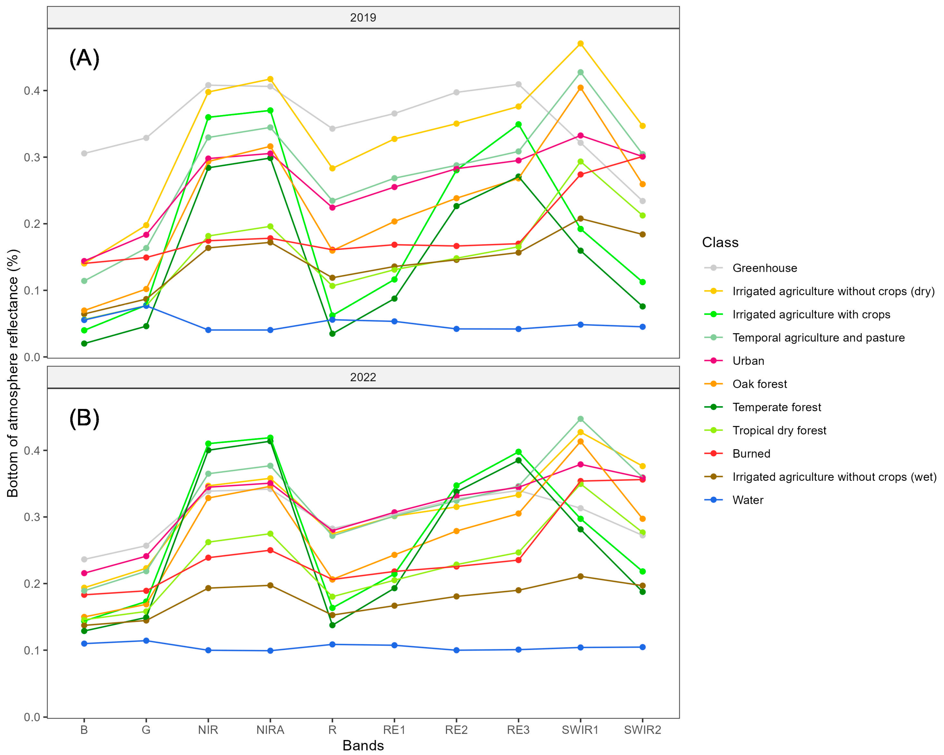
Training samples were collected for the eleven land use/land cover classes (Table 2), using Sentinel-2A images and high spatial resolution images in Google Earth (GE) as reference. The number of training samples for the 2019 and 2022 imagery is presented in the last column of Table 2. 
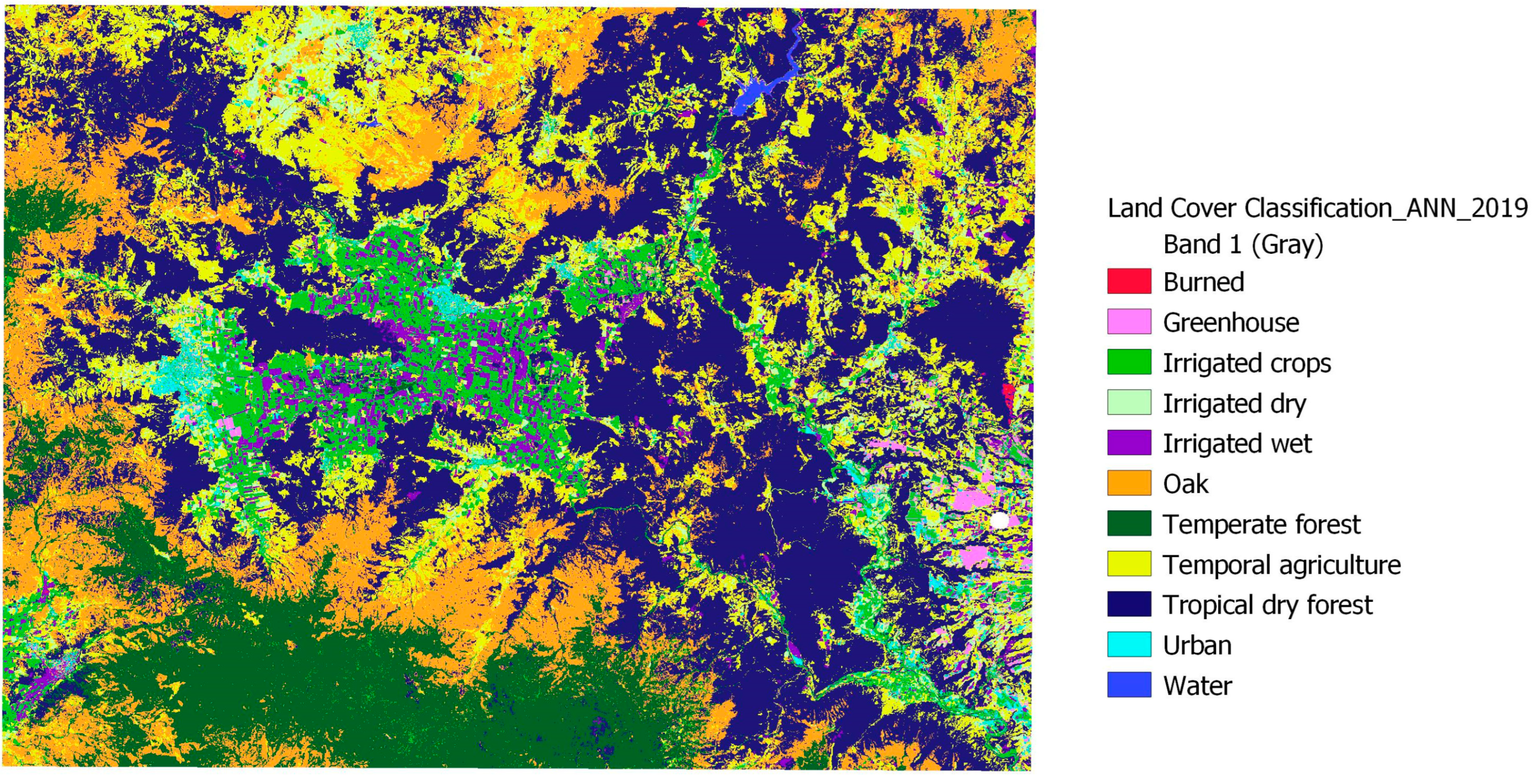
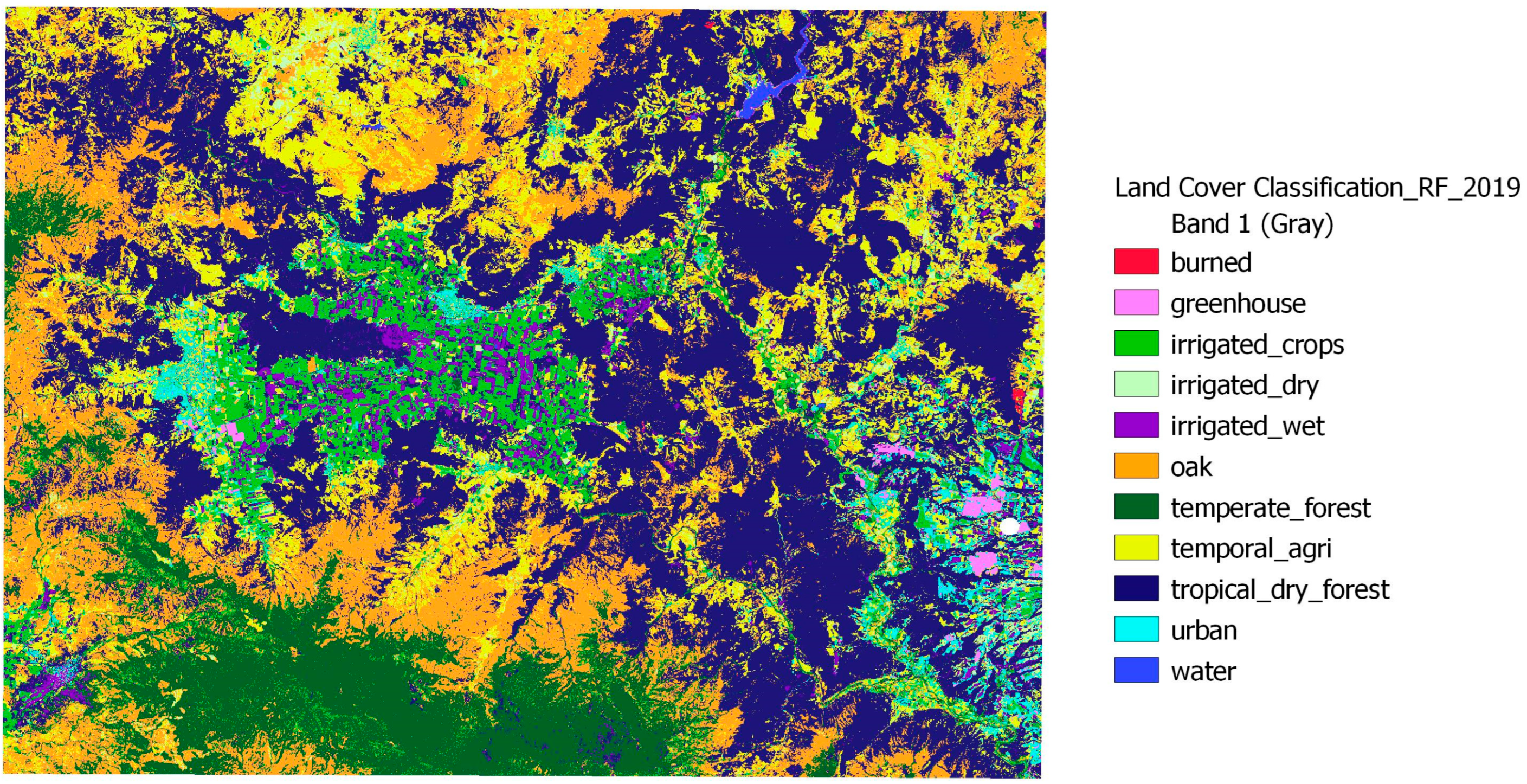
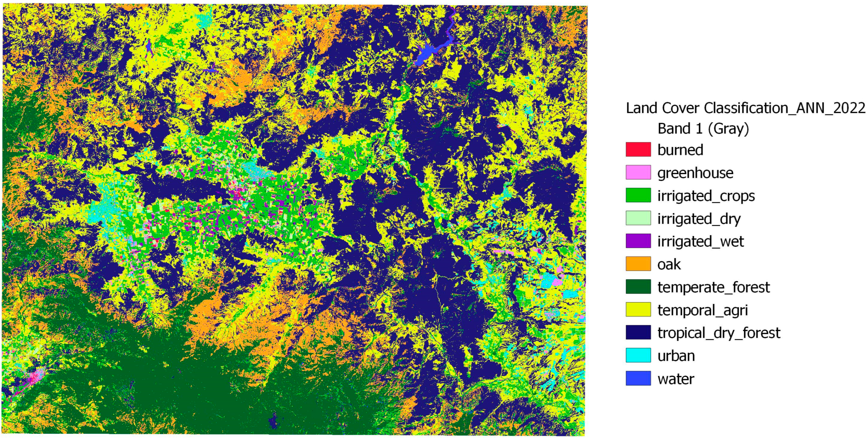
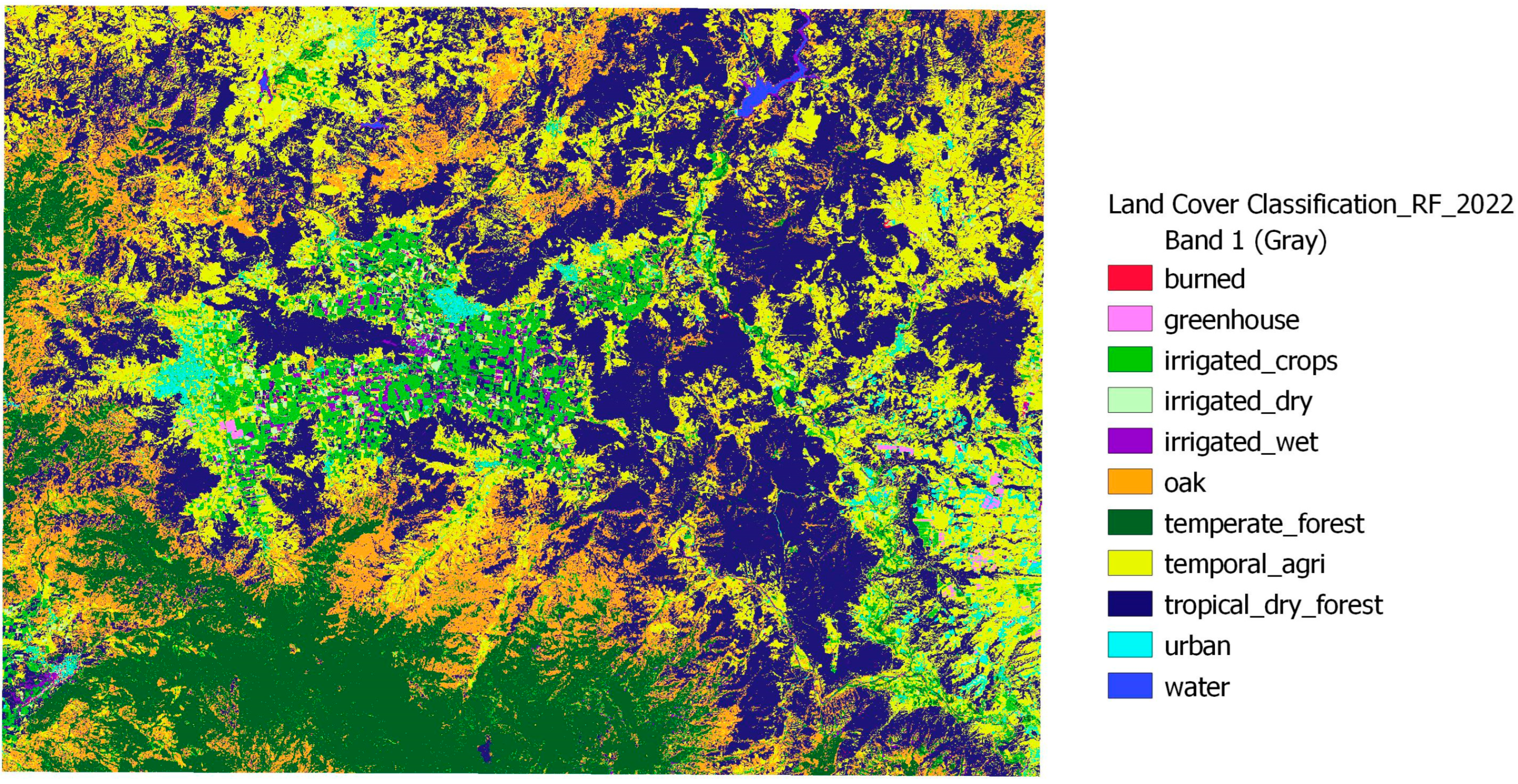
Figure 2 shows the distribution of the sample classes in Sentinel-2A bands. We also referred to the INEGI land use land cover and vegetation maps, series VII (1:250,000), which was produced during the period of 2015–2017 for the spatial distribution of different types of forests and agriculture. The distribution of TDF and oak and pine forests shows a general ascending pattern following elevation. We used two classification algorithms, namely artificial neural network and random forest, to classify the Sentinel-2A images in 2019 and 2022.

2.3.1. Artificial Neural Network

Artificial neural network (ANN) is a machine learning algorithm that uses a network of nodes to perform supervised classifications [22,23]. Typically, each neuron in an ANN receives a series of inputs, and then performs a weighted sum of them and outputs a value of 1 if its sum is over a threshold and a value of 0 if not. Finally, the complete network can classify a different set of inputs based on the neuron’s weights [24]. Training a neural network requires that the user specifies the network structure and sets the learning parameters [22]. In our case, to train the ANN, the sample data were split in the proportion of 0.7, with 70% of the data assigned as training data and the remaining 30% as test data. This algorithm applied a 5-fold cross-validation (CV) with 5 repetitions.
A 5-fold CV involves randomly dividing the training data into 5 groups, or folds, of approximately equal size [25]. The first fold is treated as a validation set, and the method is fit on the remaining 4 folds. The mean squared error, MSE, is computed with the data in the held-out fold. The process resulted in 5 estimates of the test error and the 5-fold CV estimate is computed by averaging these errors (Equation (1)).
CV 5 = 1 / 5 i = 1 5 MSE i

2.3.2. Random Forest

Random forest (RF) is a non-parametric machine learning algorithm that generates robust predictions by creating a set of regression trees from the bootstrap sampling of the original data and improving prediction accuracy by aggregating the results [26]. RF has been shown to be resistant to problems of overfitting and noise, and it has been widely used for the supervised classification of land use and land cover [27,
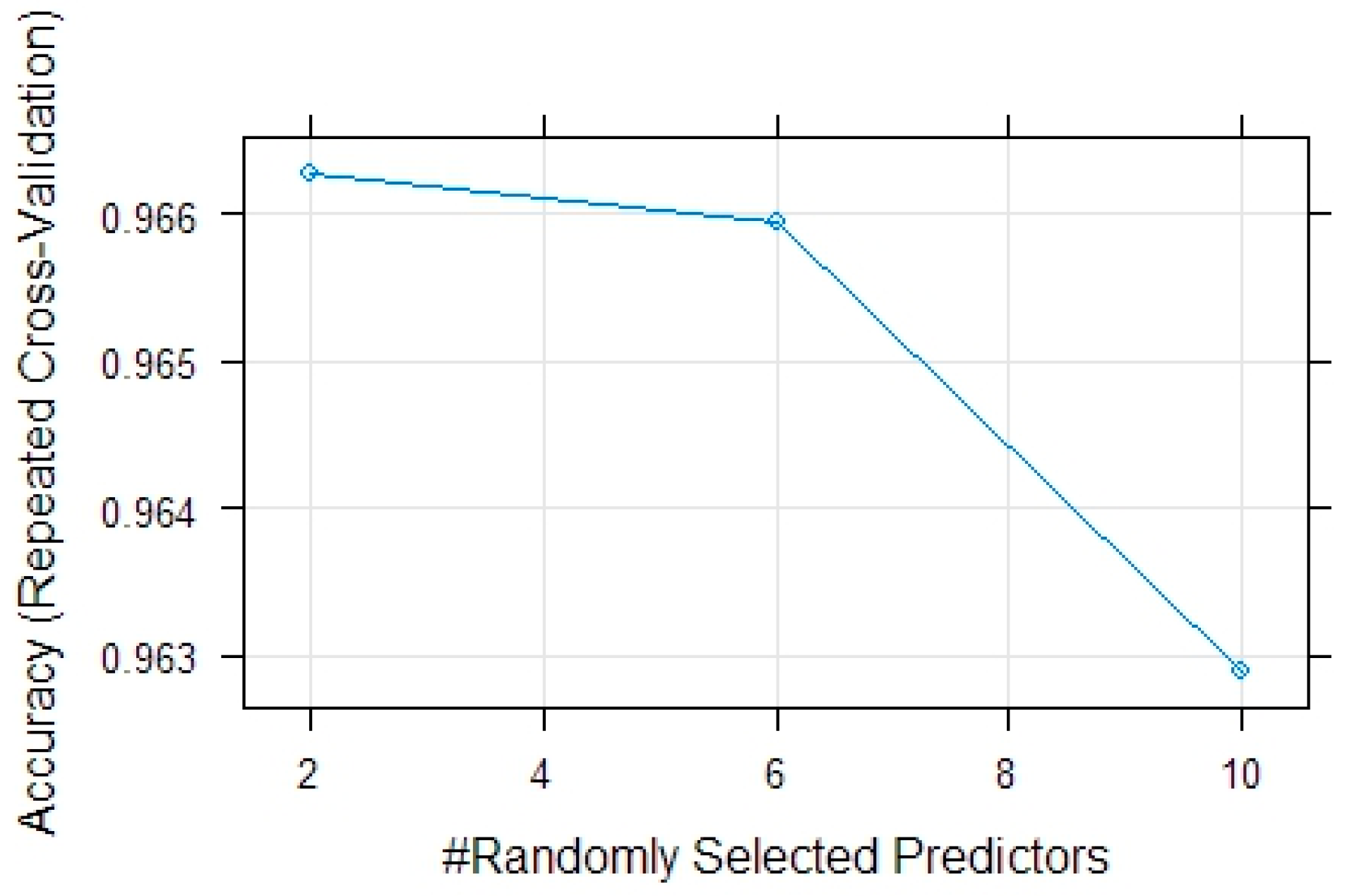
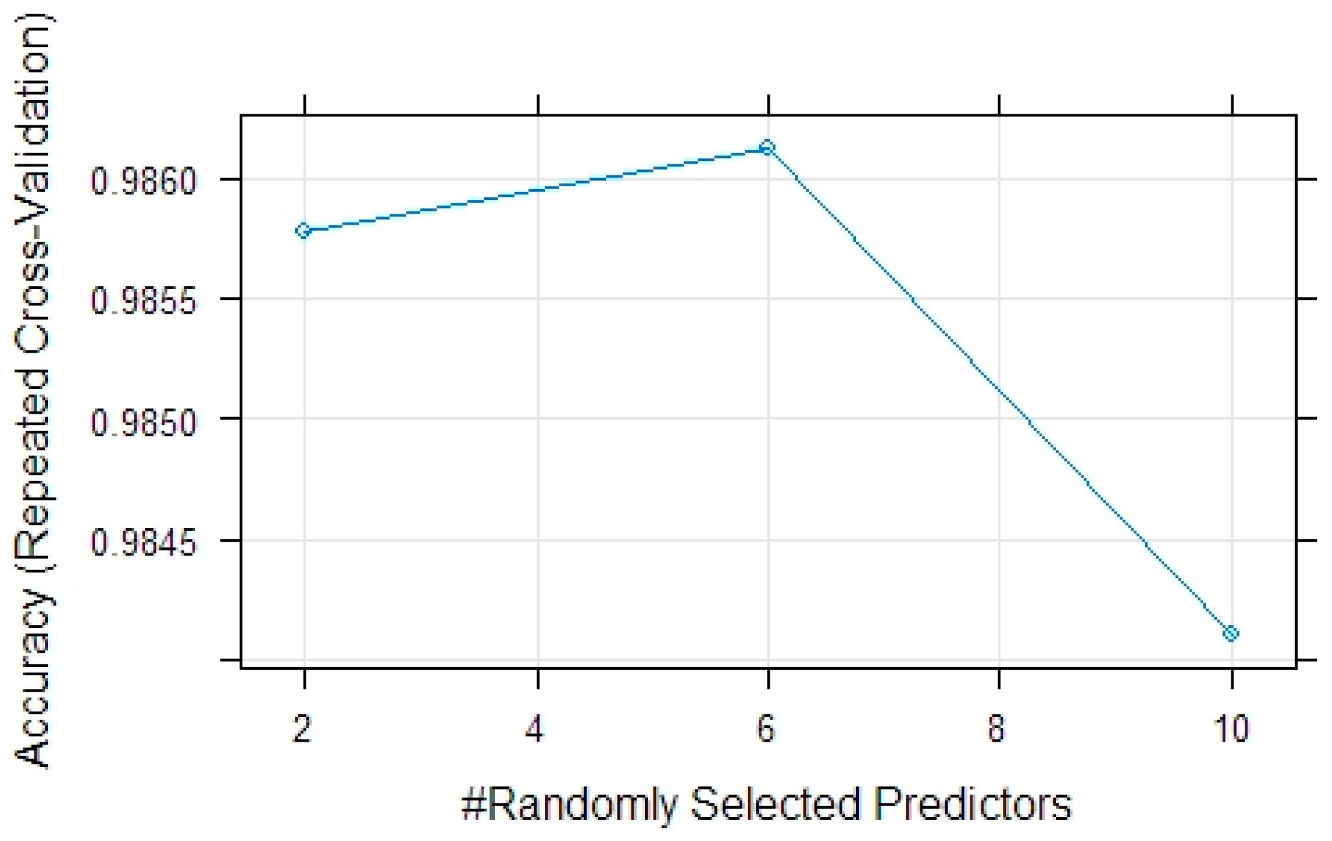
28]. In this study, we used RF to classify land use/land cover types of the study area in 2019 and 2022 using Sentinel-2A images. The sample was split with a proportion of 0.2, with 20% of the samples used as training data and the remaining 80% as test data. The tuning parameters were tested for the number of variables randomly sampled as candidates at each split (mtry: 2, 6, 10) and accuracy was used to select the optimal model. The final value used for the model of the 2022 image classification was mtry = 2 (Figure A1), and for the model of the 2019 image classification, the value was mtry = 6 (Figure A2). The “rf” method uses a default ntree of 500, which is a recommended value for remote sensing applications [29].
Consistent with the ANN classification algorithm, the RF algorithm also applied 5-fold cross-validation with 5 repetitions.

2.4. Change Analysis

We first reclassified the land use/land cover maps in 2019 and 2022 by grouping the classes of irrigated agriculture, temporal agriculture, greenhouse, and burned area into the class of agriculture, and by grouping water and urban into the class other (Table 2). The class burned area was grouped into the agriculture class because burning is part of the shifting cultivation and temporal agriculture field preparation practice [30]. The reclassified land use/land cover maps had five classes, namely TDF, temperate forest, oak forest, agriculture, and other.
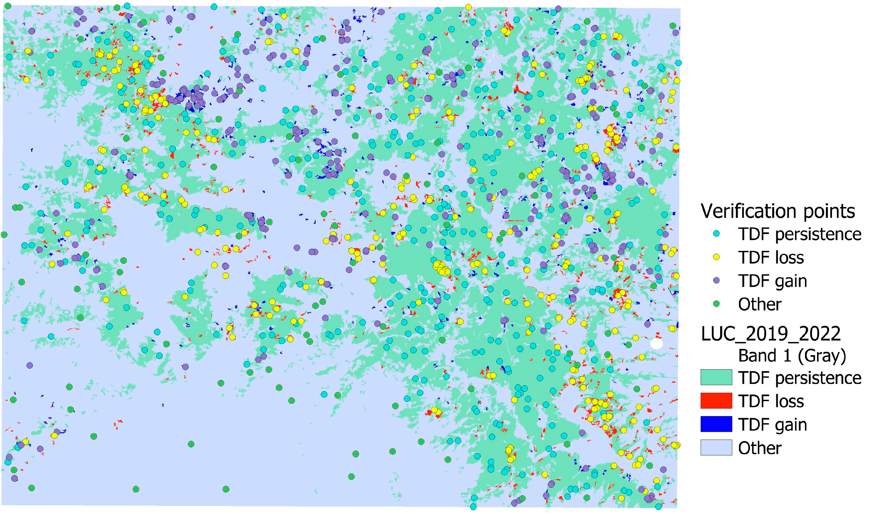
We performed the LULCC by overlaying and comparing the reclassified maps in 2019 and 2022. To analyze the dynamics of TDF, we focused on the following classes of changes and persistence: TDF persistence (35.1% of the study area), TDF loss to agriculture (1.7%), TDF gain from agriculture (1.1%), and other changes (62.1%). To remove the noise, we applied a filter of 2 ha since the average size of shifting cultivation was recorded as 2.5 ha and applied a 4-neighbor rule (QGIS sieve function) since it obtained better results.

2.5. Accuracy Assessment

Since classification errors often propagate to the result of change analysis, especially with post-classification comparison, it is important to evaluate the accuracy of the map of change in addition to the classifications. In a map of change detection, the classes of change usually occupy small proportions in comparison to the classes of persistence, and therefore, omission errors in the classes of change classes are often exaggerated due to the imbalance in area proportions and cause big uncertainty in the estimation of accuracy and areas. To counterbalance this effect, we implemented the method that was detailed in [31]. We created a buffer area the size of 12 pixels around the classes of change, assuming changes are more prone to occur in the buffer areas, and assigned 75 points to the class of TDF persistence and 75 points to the class other persistence. Following stratified random sampling [32], and assuming the standard error of the change map as 0.01, the user’s accuracy of TDF persistence 84%, TDF loss 60%, TDF gain 50%, and other 90%, and counting the 150 points from the buffer areas, the total number of random points needed for a statistically valid accuracy assessment was 1178 points. The points were distributed as follows: 331 points in TDF persistence, 300 points in TDF gain, 300 points in TDF loss, and 93 points in other persistence. The distribution of the verification points is shown in Figure 3.
We exported those points to Google Earth and interpreted them visually to obtain the ground truth data. During visual interpretation, we considered an area of 100 m2 around each point, which is equivalent to the pixel size of Sentinel-2A images. We compared the ground truth data with the map of LULCC and verified the obtained changes and persistence. We summarized the results of the accuracy assessment in an error matrix. We incorporated the area proportion of the mapped changes and calculated the overall accuracy, producer’s accuracy, and user’s accuracy with confidence intervals (CIs) and estimated the weighted areas of TDF loss and gain with their respective CIs. The accuracy assessment was carried out using Open Foris tools developed by the FAO (https://github.com/openforis/accuracy-assessment/ (accessed on 15 December 2022)).

2.6. Examining the Spatial Variables Contributing to TDF Loss and Gain

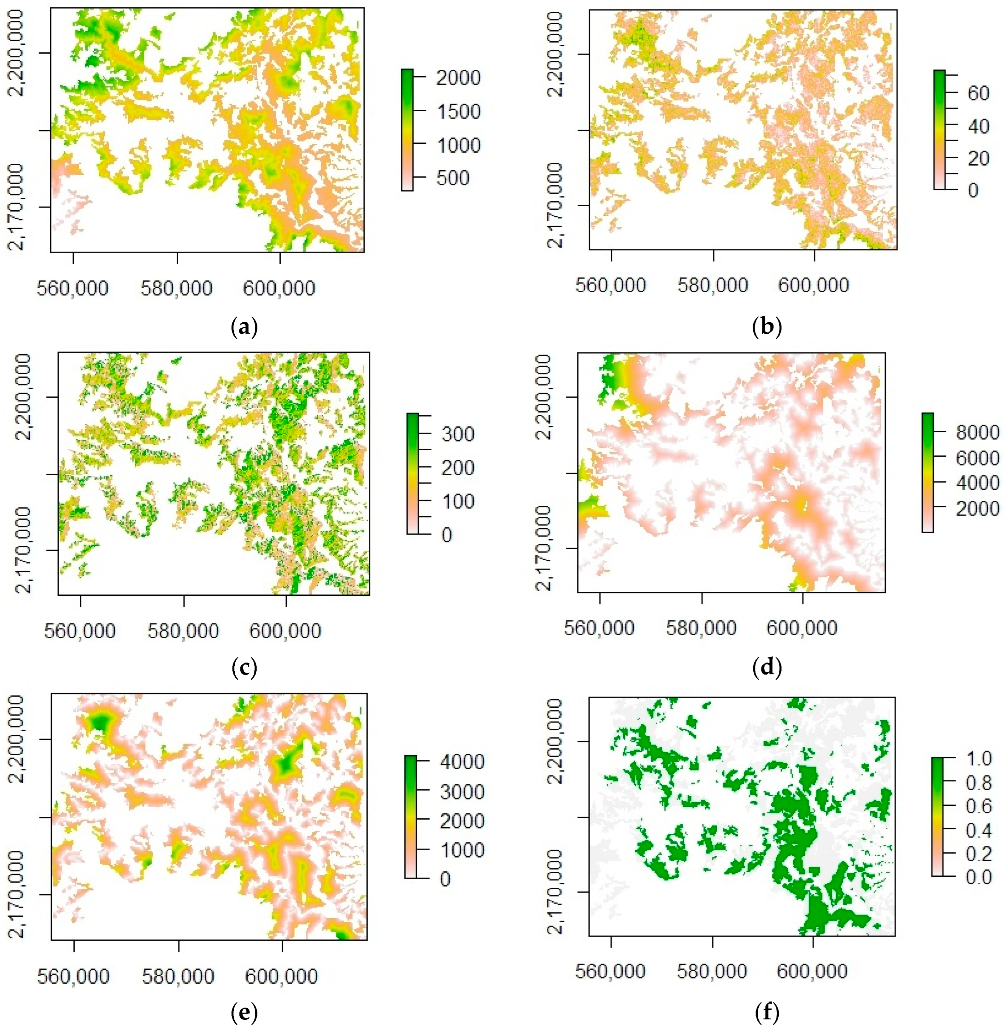
We used the verified points of TDF change and persistence to analyze the effect of spatial variables on TDF dynamics (loss to and gain from shifting cultivation). We considered topographic variables, such as elevation, aspect, and slope, and anthropogenic variables, such as distance to roads and distance to agriculture and land tenure represented by ejido and communal lands or other land ownership (Table 1). The spatial variables were resampled to 10 m spatial resolution to be consistent with the LULCC maps. We fitted two types of logistic regression models, one for TDF loss and the other for TDF gain. In these models, the dependent variables were change (1) and persistence (0), and the independent variables are the spatial variables (Figure 4).
First, we fitted the models including all the spatial variables to detect the significant terms, and then we fitted additional models using only the significant terms. We used the Akaike information criterion (AIC) to select the best model (Equation (2)). AIC is calculated using the number of independent variables (K) and the log-likelihood estimate of the model (L). Using AIC as a criterion, the best model would explain the biggest amount of variation in the data using the smallest number of independent variables [33]. We selected the best model that had the lowest AIC and was at least two units lower than the AICs of other competing models.
AIC = 2 K 2 ln ( L )
Before fitting the models, a Pearson correlation analysis was performed to avoid using strongly colinear variables in the models. A Pearson correlation coefficient of ≥0.8 was interpreted as an indicator of strongly collinear variables.
The TDF loss models had 94 verified random points for TDF loss and TDF persistence, respectively, with the explicative variables extracted to each of these 188 points. The TDF gain models had 46 verified random points for TDF gain and persistence, respectively, also with the variables extracted to each of those 92 points. Both TDF loss and TDF gain points were a subset of the verification dataset for the change analysis.

2.7. Projecting Future TDF Loss and Gain

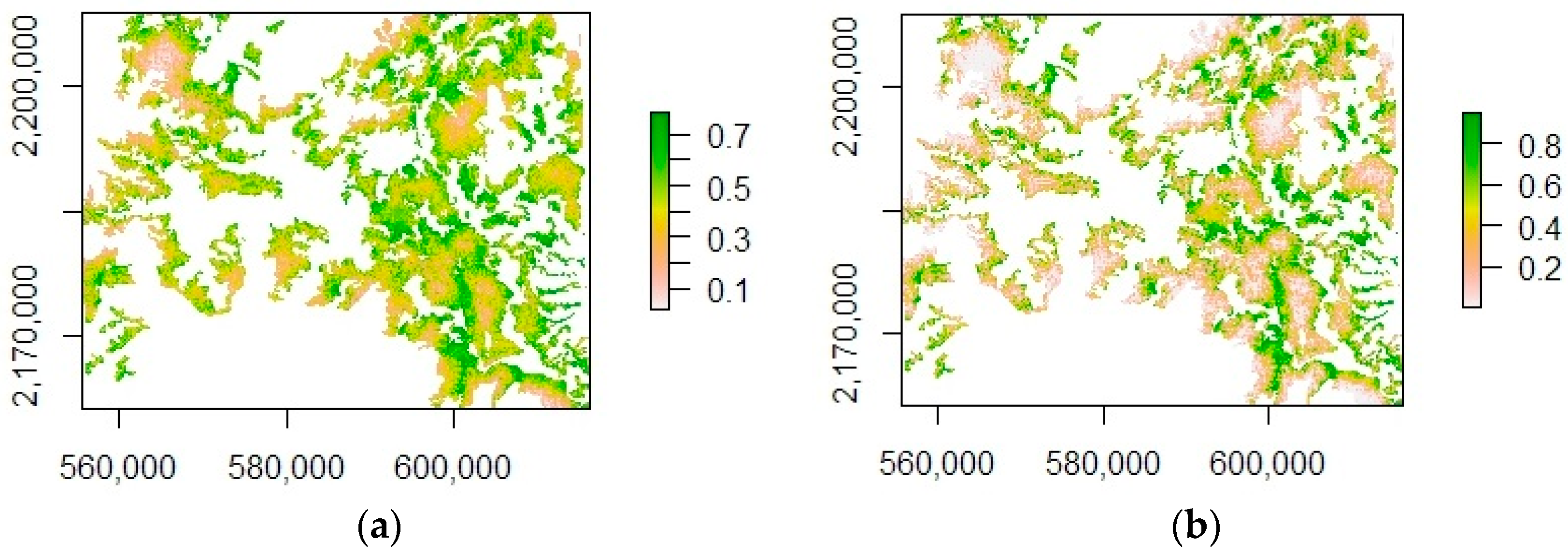
We predicted the probability of the occurrence of TDF loss and TDF gain using the best models. We reclassified the probability maps using a threshold of 0.5 and calculated the map areas with a probability higher than 0.5 as predicted areas of TDF loss or TDF gain.

2.8. Comparison of Forest Loss and Gain

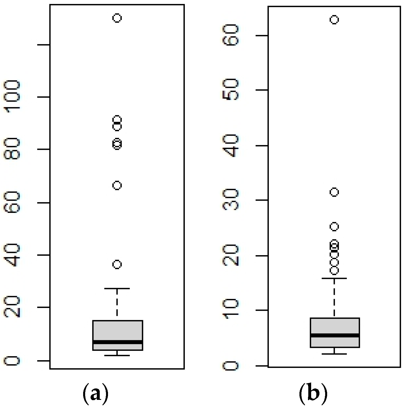
We compared the TDF loss and TDF gain by computing the statistics of their patch size and distribution. We assumed that smaller areas of forest loss might be related to areas under a shifting cultivation scheme (around 2.5 ha), contrary to larger areas of forest loss, which might be related to large-scale agricultural management. Thus, we expected a smaller area in TDF gain in comparison to TDF loss. We used a non-parametric Mann–Whitney test to test the difference between the median values of the areas of the TDF loss and TDF gain [34].

3. Results

This section presents the results of the classification accuracy assessment, change detection, influencing factors modeling with the logistic regression model, and future projection of TDF loss and gain.

3.1. Classification Model Validation

The accuracy of the classification result was evaluated with the test data using an error matrix (Appendix A Table A1, Table A2, Table A3 and Table A4). The classification of the 2019 image using the ANN obtained an overall accuracy of 0.9714 with a 95% CI of (0.9695, 0.9732), and using the RF, the classification obtained an overall accuracy of 0.9901 with a 95% CI of (0.9894, 0.9908). The classification of the 2022 image using the ANN obtained an overall accuracy of 0.9452 with a 95% CI of (0.9423, 0.948), and using the RF, the classification obtained an overall accuracy of 0.9766 with a 95% CI of (0.9754, 0.9777).
Based on the accuracy assessment, both ANN and RF achieved high overall accuracy with comparable results (Table A1, Table A2, Table A3 and Table A4). However, for both dates, the classified land use/land cover maps obtained using the ANN had less of a salt and pepper effect and there was less confusion between temperate forest and irrigated agriculture, especially in the southern part of the maps (Figure A3, Figure A4, Figure A5 and Figure A6). For this reason, we chose the results obtained using the ANN for the change analysis.

3.2. Verification of Detected Changes

The error matrix is presented in Table 3. The overall accuracy of the map of change was 0.882 ± 0.018. The unweighted producer’s accuracy for TDF loss was 0.981 and for TDF gain was 0.967, while the user’s accuracy for TDF loss was 0.503 and for TDF gain was 0.193.

3.3. Tropical Dry Forest Loss

The model for TDF loss had 188 points, 94 points for loss, and 94 points for persistence. Pearson correlation showed only a mild correlation (coefficient < 0.5) between the variables (Table A5), and, therefore, all the variables were included in the logistic regression model. We scaled all the numeric variables using the mean and the standard deviation (STD) of the samples before running the models, i.e., by subtracting the mean and dividing the STD. The logistic regression model with all variables showed that slope was significant at the 0.05 level, and distance to roads was significant at the 0.1 level (Table 4). We built another two models, one with the two significant variables (Table 5) and the other one with only slope since it had a higher coefficient (Table 6). We selected the best model with the lowest AIC (Table 5).

3.4. Tropical Dry Forest Gain

The model for TDF gain had 92 points, with 46 points for TDF gain and 46 points for persistence. The predictive variables were extracted to the location of each of these points. Two points for gain were deleted since they had NA values in the variable aspect. The final dataset had 90 points, including 44 points for gain and 46 points for persistence. The Pearson correlation showed a mild correlation between the variables, with the highest correlation being 0.66 between distance to agriculture and elevation (Table A6). The correlation was also found in the TDF loss dataset, with lower coefficient (0.53). We scaled all the numeric explicative variables similar to the procedure in the TDF loss models.
We tested the logistic regression model with all variables (Table 7). Both the distance to roads and slope were significant with negative coefficients, showing that the probability of TDF gain decreased with the increase in distance to roads and slope. We tested two more models, first with the two significant variables (Table 8) and then with the variable that had the highest coefficient (Table 9). When using only slope and distance to roads, the AIC of the model decreased (Table 8). We selected the best model with the lowest AIC for TDF gain.

3.5. Probability of Future Tropical Dry Forest Loss and Gain

The probability of future TDF loss and TDF gain were predicted with the best models (Figure 5). For both TDF loss and gain, the best models included slope and distance to roads, although in the model of TDF gain, both variables had higher coefficients (Table 8).
The potential areas of TDF loss and gain were predicted by reclassifying the probability maps with a threshold of 0.5 (Table A7). Overall, 43.1% of the total TDF area was predicted as TDF loss and 35.4% as TDF gain (Table A7), showing that TDF loss was a dominant process in the study area. This pattern coincides with the area estimates for loss and gain, although their CIs overlapped (Table 3).

3.6. Comparison of the Verified Forest Loss and Gain

The statistics for TDF loss showed a median size of 7.2 ha, an average of 14.3 ha, a minimum of 2.1, and a maximum of 130 ha. In comparison, the statistics for TDF gain showed a smaller size with a median of 5.3 ha, an average of 9 ha, a minimum of 2.2 ha, and a maximum of 62.8 ha. Despite being apparently larger in size, TDF loss in patch sizes is not significantly different from TDF gain, based on the Wilcox test for samples with a non-parametric distribution, with a p-value = 0.083. The size distribution of the TDF loss and TDF gain is shown with the boxplot in Figure 6.

4. Discussion

4.1. TDF Dynamics

During 2019–2022, in our study area, the average TDF loss and TDF gain were estimated at 6235 ha and 2784 ha, respectively, and the average rate of TDF loss and TDF gain was estimated at 1.6% and 0.7% per year, respectively. The rate of TDF loss was higher than the national level TDF loss estimated at 0.4% per year by [10], but it was comparable with the annual TDF loss rate of 1.4% at the regional level estimated by [12]. As for TDF gain, we did not find studies at the national or regional level to compare with. Both the areas and the rate of TDF loss were much higher than TDF gain. Nonetheless, the confidence intervals of the estimated areas of both classes overlapped; thus, we cannot be sure that there is a significant difference between both estimates. According to our results, TDF gain and loss are in equilibrium in the region. However, due to the relatively large confidence intervals for both area estimates, we recommend taking this conclusion with precaution.
Having smaller patch sizes, areas of TDF gain can be more readily related to TDF regrowth during the fallow period of shifting cultivation. On the other hand, large patches of TDF loss (around or more than 80 ha) are more readily related to large-scale plantations, which might not be under a shifting cultivation scheme. According to our results, the area of TDF loss and gain were not significantly different. Therefore, although large-scale plantations are more common in the study site, most of the TDF loss areas seem to be related to small-scale areas, probably under shifting cultivation or other management that could further imply a TDF recovery.
Processes such as shifting cultivation do not affect net vegetation distribution; however, they can result in an overall decrease in vegetation density and cause carbon release into the atmosphere and affect the carbon budget [20]. For TDF regeneration, assisted natural regeneration—a practice to convert degraded forests into more productive forests with improved ecosystem services by managing regeneration rather than relying on pure natural processes—is recommended [35,36]. Although this study consists of an evaluation of TDF gain and loss in terms of area, a more detailed analysis should be made to obtain the carbon balance in the study area.
As for the contributing factors, for TDF loss, both slope and distance to roads were significant predictive variables, with slope having a higher coefficient. Both variables had negative coefficients, showing that with the increase in either slope or distance to roads, the probability of TDF being converted to agriculture decreases. For TDF gain, the same variables were significant and with negative coefficients, showing that with the increase in slope and distance to roads, the probability of TDF recovery decreases. Interestingly, in both models, slope had a higher coefficient and therefore is a more important factor to determine the probability of both TDF loss and gain. In the case of TDF loss, this pattern is probably related to the fact that frequently areas with higher slopes and farther away from established roads are not preferred to establish agricultural or livestock activities, due to the costs and difficulties associated with the transportation of products and animals to those areas. In the case of TDF gain, its dependence on TDF loss (i.e., for an area to gain TDF, first it must lose it) causes the same relation with those two variables.

4.2. Methodological Challenges and Insights

The wide range in area estimation of TDF loss and TDF gain partly comes from the fact that these two change classes occupied a small proportion of the area in comparison to classes of persistence, and therefore, (small) a number of omission errors were exaggerated due to the imbalance in area proportions. We intended to counteract this imbalance in area proportion by creating buffer zones of 12 pixels of Sentinel-2A images (120 m) around the change areas, assuming that omission errors are prone to occur near detected changes [31]. However, we did not succeed in reducing the confidence intervals. One possible reason could be that the buffer size is not wide enough to cover the points of omission errors. For future work, we will consider using different buffer sizes to find out how buffer size affects the reduction in omission errors.
The maps of predicted forest loss and gain created using our models show that forest loss and gain follow a similar spatial distribution because of their dependence on the same explicative variables: slope and distance to roads. These maps were created using a limited number of factors including slope, elevation, and distance to roads; thus, other plausible factors that might explain forest loss and gain were omitted. For example, factors related to the presence of large-scale agriculture companies or certain governmental incentives. Nonetheless, our maps can give a general idea of which areas are prone to being under shifting cultivation management.
We analyzed TDF dynamics for a rather short time window (2019–2022). Although we could capture the TDF gain and loss from shifting cultivation, an analysis with a longer time span, e.g., 10–30 years, could potentially allow us to have a more precise area estimation of TDF gain and loss (with a smaller confidence interval).
For TDF dynamics, time series analysis of climate data (air temperature, precipitation) is useful to exempt false changes introduced by climate variations. Table 10 shows the annual average temperature and annual precipitation for our study area. The precipitation data were derived from CHIRPS “Climate Hazards Group InfraRed Precipitation with Station Data” and the temperature data are from MODIS “Land surface temperature”. The annual temperature was rather stable for the period of 2018–2022, while the annual precipitation showed some variation, with much higher precipitation in 2022 than in 2019 (Table 10), which could explain why the vegetation in the 2022 image was greener even in a dry season. Since we used a two-time classification comparison to analyze TDF dynamics, and we provided independent training samples for the classification at each time point, the effect of the interannual climate variations on the vegetation cover was well captured with the image classification. Since we verified the changes using visual interpretation with reference to very high spatial resolution images from Google Earth, the climate-induced effects were largely removed from contributing factor analysis of TDF dynamics.

5. Conclusions

We used multi-temporal Sentinel-2A images and topographic, anthropogenic and land tenure factors to investigate the dynamics of tropical dry forest in terms of gain and loss and the associated factors. We estimated a TDF loss rate of 1.6% per year and a TDF gain rate of 0.7% per year. Although apparently TDF loss rate was higher than TDF gain, because of the large confidence interval in our area estimate, we cannot conclude that TDF loss was more intense but rather that the TDF loss was in equilibrium with TDF gain. In future analysis, we will assess other methods that can help reduce the confidence intervals in area estimates to obtain a clearer conclusion regarding TDF loss and gain.
As for the contributing factors, both TDF loss and gain were inversely related to slope and distance to roads; therefore, these two factors explain the probability of a TDF area in both gain and loss. In the case of TDF loss, this is related to the fact that agricultural or livestock activities generally prefer flat areas for easy access and cheap cost; for TDF gain, since it depends on TDF loss, the same relation with slope could explain the distribution of TDF gain.

Author Contributions

Conceptualization, Y.G.; methodology, Y.G.; validation, Y.G. and J.V.S.; formal analysis, Y.G.; writing—original draft preparation, Y.G.; writing—review and editing, Y.G., J.V.S., R.C.E. and S.T. All authors have read and agreed to the published version of the manuscript.

Funding

This research received no external funding.

Data Availability Statement

Data are available through request to the corresponding author.

Acknowledgments

The first author would like to thank the Direccion General de Asuntos del Personal Académico (DEGAPA) at the Universidad Nacional Autónoma de México (UNAM) for the financial support.

Conflicts of Interest

The authors declare no conflict of interest.

Appendix A

BU: burned; GH: greenhouse; IC: irrigated agriculture with crops; ID: irrigated agriculture without crops (dry); IW: irrigated agriculture without crops (wet); O: oak forest; TF: temperate forest; TA: temporal agriculture and pasture; TDF: tropical dry forest; U: urban; W: water; UA: User’s accuracy; PA: Producer’s accuracy; OA: Overall accuracy.
Table A1. Error matrix for accuracy assessment of the classification in 2019 using ANN.
BUGHICIDIWOTFTATDFUWTUA
BU36600000010003670.997
GH01100000001018011190.983
IC0039591056100039720.996
ID0601260000206026014980.841
IW000016740024790017770.942
O000005987258410060880.983
TF005600144575040046490.984
TA00017462403263300034970.933
TDF000011891067290068300.985
U000730000018302560.715
W0300000000178317860.998
Total36611094015150816916119458435546883227178331,839
PA10.9920.9860.8360.990.9780.9980.9180.9780.8061
OA0.970
Table A2. Error matrix for accuracy assessment of the classification in 2019 using random forest.
BUGHICIDIWOTFTATDFUWTUA
BU95100000050009560.995
G02885000003015029030.994
IC0010,776001179002010,8680.992
ID0003924050148011040880.96
IW000044230120270044620.99
O0000016,0913311230016,2480.99
TF0047021212,148040012,2130.995
TA90012503509166342093800.977
TDF000010730518,1360018,2240.995
U010180003061506370.966
W0000000000491449141
Total960288610,8234067443516,22712,242936118,293685491484,893
PA0.9910.99960.9960.9650.9970.9920.9920.9790.9910.8981
OA0.9898
Table A3. Error matrix for accuracy assessment of the classification in 2022 using ANN.
BUGHICIDIWOTFTATDFUWTUA
BU860094000000990.869
G2199110000203102450.812
IC032031003685520021620.939
ID100310000660103780.820
IW24803200000093430.933
O0041002396249650025530.939
TF004300233094000031600.979
TA0070307057058948748064630.912
TDF1000129316176090077770.978
U0640100045034304530.757
W0000001000102310240.999
Total9227022046273362572316661727763423103224,657
PA0.9350.7370.9220.4940.9520.9320.9770.9550.9800.8110.991
OA0.945
Table A4. Error matrix for accuracy assessment of the classification in 2022 using random forest.
BUGHICIDIWOTFTATDFUWTUA
BU24700100000002480.996
G07240000060607360.984
IC005744021086904058550.981
ID100137700028011014170.972
IW000088300010118950.987
O00000645316791021066510.970
TF0011700218284000084220.984
TA11262940123016,19259109016,8050.964
TDF00001529705020,5061020,8690.983
U220000046093409840.949
W0000200000286328650.999
Total251727588716729026904838616,41020,6681066287465,747
PA0.9840.9960.9760.8240.9790.9350.9880.9870.9920.8760.996
OA0.977
Table A5. Pearson correlation between (numeric) explicative variables for TDF loss.
Explicative VariablesDistance to RoadsDistance to AgricultureElevationSlopeAspect
Distance to roads1.00
Distance to agriculture0.441.00
Elevation0.450.531.00
Slope0.310.460.351.00
Aspect0.04−0.05−0.1−0.011.00
Table A6. Pearson correlation between (numeric) explicative variables for TDF gain.
Explicative VariablesDistance to RoadsDistance to AgricultureElevationSlopeAspect
Distance to roads1.00
Distance to agriculture0.421.00
Elevation0.480.661.00
Slope0.330.330.291.00
Aspect0.030.00−0.02−0.061.00
Table A7. Reclassified probabilities of TDF loss and gain using a threshold of 0.5.
Reclassified ProbabilitiesNo. of PixelsPercentageReclassified ProbabilitiesNo. of PixelsPercentage
0.5, 0.788 (TDF loss)4,798,43643.08%0.5, 0.953 (TDF gain)3,941,96435.39%
0.017, 0.56,340,49856.92%0.00002, 0.57,196,97064.61%
Total11,138,9341Total11,138,9341

Appendix B

Figure A1. Cross-validation for the classification of Sentinel-2 imagery in 2022 with tested mtry = 2, 6, and 10. Mtry = 2 was selected for its highest accuracy.
Remotesensing 15 01471 g0a1
Figure A2. Cross-validation for the classification of Sentinel-2 imagery in 2019 with tested mtry = 2, 6, and 10. Mtry = 6 was selected for its highest accuracy.
Remotesensing 15 01471 g0a2
Figure A3. Land cover classification using ANN for 2019. Irrigated crops is short for Irrigated agriculture with crops; Irrigated dry is short for Irrigated agriculture without crops (dry); Irrigated wet is short for Irrigated agriculture without crops (wet); Temporal agriculture is short for Temporal agriculture with pasture; Oak is short for Oak forest.
Remotesensing 15 01471 g0a3
Figure A4. Land cover classification using random forest (RF) for 2019. Irrigated crops is short for Irrigated agriculture with crops; Irrigated dry is short for Irrigated agriculture without crops (dry); Irrigated wet is short for Irrigated agriculture without crops (wet); Temporal agriculture is short for Temporal agriculture with pasture; Oak is short for Oak forest.
Remotesensing 15 01471 g0a4
Figure A5. Land cover classification using ANN for 2022. Irrigated crops is short for Irrigated agriculture with crops; Irrigated dry is short for Irrigated agriculture without crops (dry); Irrigated wet is short for Irrigated agriculture without crops (wet); Temporal agriculture is short for Temporal agriculture with pasture; Oak is short for Oak forest.
Remotesensing 15 01471 g0a5
Figure A6. Land cover classification using random forest (RF) for 2022. Irrigated crops is short for Irrigated agriculture with crops; Irrigated dry is short for Irrigated agriculture without crops (dry); Irrigated wet is short for Irrigated agriculture without crops (wet); Temporal agriculture is short for Temporal agriculture with pasture; Oak is short for Oak forest.
Remotesensing 15 01471 g0a6

References

  1. Olson, D.M.; Dinerstein, E.; Wikramanayake, E.D.; Burgess, N.D.; Powell, G.V.N.; Underwood, E.C.; D’Amico, J.A.; Itoua, I.; Strand, H.E.; Morrison, J.C.; et al. Terrestrial ecoregions of the world: A new map of life on Earth. BioScience 2001, 51, 933–938. [Google Scholar] [CrossRef]
  2. Rzedowski, J. Vegetaci6n de Mexico; Edicion digital; Comisión Nacional para el Conocimiento y Uso de la Biodiversidad: Ciudad de México, México, 2006; 504p. [Google Scholar]
  3. Maass, J.; Balvanera, P.; Castillo, A.; Daily, G.; Mooney, H.; Ehrlich, P.; Quesada, M.; Miranda, A.; Jaramillo, V.; García-Oliva, F.; et al. Ecosystem services of tropical dry forests: Insights from long-term ecological and social research on the Pacific Coast of Mexico. Ecol. Soc. 2005, 10, 17. Available online: http://www.ecologyandsocity.org/vol10/iss1/art17/ (accessed on 7 November 2022). [CrossRef]
  4. Pennington, R.T.; Lavin, M.; Oliveira-Filho, A. Woody plant diversity, evolution, and ecology in the tropics: Perspectives from seasonally dry tropical forests. Annu. Rev. Ecol. Evol. Syst. 2009, 40, 437–457. [Google Scholar] [CrossRef] [Green Version]
  5. Caballos, G.; Ceballos, G.; Andres Garcia, A. Conserving Neotropical Biodiversity: The Role of Dry Forests in Western Mexico. Conserv. Biol. 1995, 9, 1349–1353. Available online: https://www.jstor.org/stable/2387179 (accessed on 7 November 2022). [CrossRef]
  6. Mesa-Sierre, N.; de la Peña-Domene, M.; Campo, J.; Giardina, C.P. Restoring Mexican Tropical Dry Forests: A National Review. Sustainability 2022, 14, 3937. [Google Scholar] [CrossRef]
  7. Meave, J.A.; Romero-Romero, M.A.; Salas-Morales, S.H.; Pérez-García, E.A.; Gallardo-Cruz, J.A. Diversidad, amenazas y oportunidades para la conservación del bosque tropical caducifolio en el estado de Oaxaca, México. Ecosistemas 2012, 21, 85–100. [Google Scholar]
  8. Le Quéré, C.; Moriarty, R.; Andrew, R.M.; Peters, G.P.; Ciais, P.; Friedlingstein, P.; Jones, S.D. Global carbon budget 2014. Earth Syst. Sci. Data 2015, 7, 47–85. [Google Scholar] [CrossRef] [Green Version]
  9. Gasser, T.; Crepin, L.; Quilcaille, Y.; Houghton, R.A.; Ciais, P.; Obersteiner, M. Historical CO2 emissions from land use and land cover change and their uncertainty. Biogeosciences 2020, 17, 4075–4101. [Google Scholar] [CrossRef]
  10. Mas, J.F.; Velázquez, A.; Díaz-gallegos, J.R.; Mayorga-Saucedo, R.; Alcántara, C.; Bocco, G.; Castro, R.; Fernández, T.; Pérez-Vega, A. Assessing land use/cover changes: A nationwide multidate spatial database for Mexico. Int. J. Appl. Earth. Obs. Geoinf. 2004, 5, 249e261. [Google Scholar] [CrossRef]
  11. Trejo, I.; Dirzo, R. Deforestation of seasonally dry tropical forest: A national and local analysis in Mexico. Biol. Conserv. 2000, 94, 133–142. [Google Scholar] [CrossRef]
  12. Chazdon, R.L. Tropical forest recovery: Legacies of human impact and natural disturbances. Perspect. Plant Ecol. Evol. Syst. 2003, 6, 51–71. [Google Scholar] [CrossRef] [Green Version]
  13. Morales-Barquero, L.; Borrego, A.; Skutsch, M.; Kleinn, C.; Healey, J.R. Identification and Quantification of Drivers of Forest Degradation in TropicalDry Forests: A Case Study in Western Mexico. Land Use Policy 2015, 49, 296–309. [Google Scholar] [CrossRef] [Green Version]
  14. Borrego, A.; Skutsch, M. How Socio-Economic Differences betweenFarmers Affect Forest Degradation in Western Mexico. Forests 2019, 10, 893. [Google Scholar] [CrossRef] [Green Version]
  15. Heinimann, A.; Mertz, O.; Frolking, S.; Egelund Christensen, A.; Hurni, K.; Sedano, F.; Chini, L.P.; Sahajpal, R.; Hansen, M.; Hurtt, G. A global view of shifting cultivation: Recent, current, and future extent. PLoS ONE 2017, 12, e0184479. [Google Scholar] [CrossRef] [Green Version]
  16. Hillel, D. Soil and Water Management. In Soil in the Environment; Hillel, D., Ed.; Academic Press: Cambridge, MA, USA, 2008; pp. 175–195. [Google Scholar] [CrossRef]
  17. Hartter, J.; Lucas, C.; Gaughan, A.E.; Lizama, L. Detecting tropical dry forest succession in a shifting cultivation mosaic of the Yucatán Peninsula, Mexico. Appl. Geogr. 2008, 28, 134–149. [Google Scholar] [CrossRef]
  18. Borrego, A.; Skutsch, M. Estimating the opportunity costs of activities that cause degradation in tropical dry forest: Implications for REDD+. Ecol. Econ. 2014, 101, 1–9. [Google Scholar] [CrossRef]
  19. Olofsson, J.; Hickler, T. Effects of human land-use on the global carbon cycle during the last 6000 years. Veg. Hist. Archaeobot. 2008, 17, 605–615. [Google Scholar] [CrossRef] [Green Version]
  20. Comisión Nacional Forestal. Visión de México Sobre REDD+: Hacia una Estrategia Nacional; Comisión Nacional Forestal: Zapopan, México, 2010. [Google Scholar]
  21. Cuevas, R.; Nuñez, N.M. El bosque tropical caducifolio en la Reserva de la Biosfera Sierra Manantlan, Jalisco-Colima, Mexico. Bol. Inst. Bot. Univ. Guadalaj. 1998, 5, 445–491. [Google Scholar]
  22. Kavzoglu, T.; Mather, P.M. The use of backpropagating artificial neural networks in land cover classification. Int. J. Remote Sens. 2008, 24, 4907–4938. [Google Scholar] [CrossRef]
  23. Mas, J.F.; Puig, H.; Palacio, J.L.; Sosa-Lopez, A. Modelling deforestation using GIS and artificial neural networks. Environ. Model. Softw. 2004, 19, 461–471. [Google Scholar] [CrossRef]
  24. Krogh, A. What are artificial neural networks? Nat. Biotechnol. 2008, 26, 195–197. [Google Scholar] [CrossRef] [PubMed]
  25. James, G.; Witten, D.; Hastie, T.; Tibshirani, R. An Introduction to Statistical Learning, with Applications in R, 2nd ed.; Springer: Berlin/Heidelberg, Germany, 2021. [Google Scholar]
  26. Breiman, L. Random Forests. Mach. Learn. 2001, 45, 5–32. [Google Scholar] [CrossRef] [Green Version]
  27. Gomez, C.; White, J.C.; Wulder, M.A. Optical remotely sensed time series data for land cover classification: A review. ISPRS J. Photogramm. Remote Sens. 2016, 116, 55–72. [Google Scholar] [CrossRef] [Green Version]
  28. Solórzano, J.V.; Mas, J.F.; Gao, Y.; Gallardo, A. Land use land cover classification with U-Net: Advantages of combining Sentinel-1 and Sentinel-2 imagery. Remote Sens. 2021, 13, 3600. [Google Scholar] [CrossRef]
  29. Liaw, A.; Wiener, M. Classification and Regression by randomForest. R News. 2002, 2, 18–22. [Google Scholar]
  30. Fearnside, P.M. Global Warming and Tropical Land-Use Change: Greenhouse Gas Emissions from Biomass Burning, Decomposition and Soils in Forest Conversion, Shifting Cultivation and Secondary Vegetation. Clim. Chang. 2000, 46, 115–158. [Google Scholar] [CrossRef]
  31. Olofsson, P.; Arevalo, P.; Espejo, A.B.; Green, C.; Lindquist, E.; McRoberts, R.E.; Sanz, M.J. Mitigating the effects of omission error son área and area change estimates. Remote Sens. Environ. 2020, 236, 111492. [Google Scholar] [CrossRef]
  32. Olofsson, P.; Foody, G.M.; Herold, M.; Stehman, S.V.; Woodcock, C.E. Good practices for estimating area and assessing accuracy of land change. Remote Sens. Environ. 2014, 148, 42–57. [Google Scholar] [CrossRef]
  33. Burnham, K.P.; Anderson, D.R. Model Selection and Multimodel Inference: A Practical Information-Theoretic Approach, 2nd ed.; Springer: New York, NY, USA, 2002. [Google Scholar]
  34. Wilcoxon, F. Individual comparisons by ranking methods. Biom. Bull. 1945, 1, 80–83. [Google Scholar] [CrossRef]
  35. Shono, K.; Cadaweng, E.A.; Durst, P.B. Application of Assisted Natural Regeneration to Restore Degraded Tropical Forestlands. Restor. Ecol. 2007, 15, 620–626. [Google Scholar] [CrossRef]
  36. Yang, Y.; Wang, L.; Yang, Z.; Xu, C.; Xie, J.; Chen, G.; Lin, C.; Guo, J.; Liu, X.; Xiong, D.; et al. Large Ecosystem Service Benefits of Assisted Natural Regeneration. J. Geophys. Res. Biogeosci. 2018, 123, 676–687. [Google Scholar] [CrossRef]
Figure 1. Location of the study area in the central west of Mexico. The background is a natural color composite of Landsat 8 imagery. The distribution of the tropical dry forest in the study area is shown in light green color.
Remotesensing 15 01471 g001
Figure 2. The distribution of the mean reflectance of the samples for the land use/land cover classes at the ten spectral bands of Sentinel-2 images for the years 2019 (A) and 2022 (B). Classes are sorted in descending order according to their mean reflectance in the NIR band in 2019. The standard deviations of the spectral reflectance range from 0.0042 to 0.142.
Remotesensing 15 01471 g002
Figure 3. The map of the land use land cover change (LULCC) and the distribution of the verification points.
Remotesensing 15 01471 g003
Figure 4. Explicative spatial variables: (a) elevation, (b) slope, (c) aspect, (d) distance to agriculture, (e) distance to roads, and (f) land ownership.
Remotesensing 15 01471 g004
Figure 5. Probability of TDF loss (a) and TDF gain (b) predicted with the best models. (a) Probability of TDF loss predicted with slope and distance to roads. (b) Probability of TDF gain predicted with slope and distance to roads.
Remotesensing 15 01471 g005
Figure 6. Boxplots of the patch size (ha) of (a) TDF loss patches and (b) TDF gain patches.
Remotesensing 15 01471 g006
Table 1. Datasets used.
DatasetsResolution Date/Value RangeDescriptionSource
Sentinel-2A10 m, 20 m 15 May 2019; 15 March 2022Orthorectified, radiometrically calibrated and atmospherically correctedhttps://doi.org/10.5270/S2_-znk9xsj (accessed on 12 November 2022)
Elevation15 m292–2132 m above sea levelSix scenes of Digital Elevation Model (DEM) (E13B12, E13B13, E13B14, E13B23, E13B24) to cover the study area, downloaded from https://www.inegi-org.mx/app/geo2/elevacionesmex/ (accessed on 2 December 2022)
Slope15 m0.6–73.9 (°)Arctan(rise/run)Calculated using the DEM
Aspect15 m0.0–359.76 (°)Represents the compass direction that the slope of the terrain faces. An aspect of 0 means that the slope is north-facing, 90 east-facing, 180 south-facing, and 270 west-facing.Calculated using the DEM
Distance to roads 10 m0–4235.6 (m)Euclidean distance was used to represent distance to roads. https://www.inegi.org.mx/temas/viascomunicacion (accessed on 2 December 2022)
Distance to agriculture10 m0.0–9235.4 (m)Euclidean distance was used to represent distance to agriculture. https://www.inegi.org.mx/temas/usosuelo (accessed on 2 December 2022)
Land ownership10 m1: ejido and communal.
0: other
The land ownership was categorized into two categories: both ejido and communal, and other type which cover 38.6% and 61.4% of the study area, respectively.https://www.gob.mx/ran#709 (accessed on 2 December 2022)
Table 2. Definition of land cover/land use classes (in reference to the INEGI series VII class definition).
ClassesChange ClassesClass DefinitionThe Number of Training Samples in Pixel for 2019/2022
Tropical dry forestTropical dry forestDense and sparse vegetation in different stages of succession25,883/22,876
Temperate forestTemperate forestConiferous and mountain cloud forest10,504/15,296
Oak forestOak forestForest formation distributed between tropical dry forest and temperate forest8580/20,237
Irrigated agriculture with cropsAgricultureCrops in different growing stages7307/13,581
Irrigated agriculture without crops (wet)Wet agricultural fields temporarily without crops 1116/5590
Irrigated agriculture without crops (dry)Dry agricultural fields temporarily without crops 2075/5047
GreenhouseAgriculture fields covered by greenhouse907/3632
BurnedBurned agriculture or forest area314/1226
Temporal agriculture and pastureRain-fed annual agriculture and grassland fields 20,546/11,679
WaterOtherWaterbody3573/6117
UrbanUrban landscape and scattered houses in rural areas1380/833
Table 3. Error matrix with sample points. OA: overall accuracy; PA: producer’s accuracy; UA: user’s accuracy; CI: confidence interval; MA: map area; AP: area proportion; Buffer-TDF-P: buffer in TDF persistence, Buffer-O: buffer in other.
Ground Data
TDF
persistence
TDF lossTDF gainOtherBuffer-TDF-PBuffer-OMA (ha)AP (%) UA
Map dataTDF
persistence
3340100099,93132.170.997
TDF loss0151001113848141.550.503
TDF gain0158011312830220.970.193
Other12217800176,81356.920.839
Buffer-TDF-P000071411,8433.810.947
Buffer-O0000136214,2064.570.827
Total3461546078308232310,628
PA0.9650.9810.96710.2310.267
Weighted
PA
0.814 0.389 0.2101 0.6760.823
Estimated MA (ha) with 95% CI122,447 ± 12,1266235 ± 52482784 ± 3774148,295 ± 13,28916,593 ± 140214,274 ± 1389
OA with 95% CI0.882 ± 0.018
Table 4. Result of the logistic regression predicting tropical forest loss to agriculture with all explicative variables. ‘**’ significant at 0.01 level, ‘.’ significant at 0.1 level.
VariablesEstimateStd. ErrorZ Valuep-Value
Intercept−0.03330.2062−0.1610.8717
Distance to roads−0.33950.1894−1.7920.0731 .
Distance to agriculture−0.09130.2155−0.4240.6718
Elevation−0.12820.1960−0.6540.5130
Slope−0.50040.1863−2.6850.0072 **
Aspect0.19100.15781.2100.2263
Tenure0.00560.31780.0180.9859
Null deviance: 260.62 on 187 degrees of freedom, Residual deviance: 235.37 on 181 degrees of freedom, AIC: 249.37.
Table 5. Result of the logistic regression predicting tropical forest loss to agriculture with variables of slope and distance to roads. ‘*’ Significant at 0.05 level, ‘**’ significant at 0.01 level.
VariablesEstimateStd. ErrorZ Valuep-Value
Intercept−0.02800.1556−0.1800.8575
Slope−0.56130.1752−3.2050.0014 **
Distance to roads−0.40360.1730−2.3330.0197 *
Null deviance: 260.62 on 187 degrees of freedom, Residual deviance: 238.12 on 185 degrees of freedom, AIC: 244.12.
Table 6. Result of the logistic regression predicting tropical forest loss to agriculture with the variable slope. ‘***’ Significant at 0.001 level.
VariablesEstimateStd. ErrorZ Valuep-Value
intercept−0.01540.1529−0.1010.9198
Slope−0.64540.1690−3.8180.0001 ***
Null deviance: 260.62 on 187 degrees of freedom, Residual deviance: 243.87 on 186 degrees of freedom, AIC: 247.87.
Table 7. Results of the logistic regression model predicting tropical forest gain from agriculture using all predictive variables. ‘*’ Significant at 0.05 level, ‘***’ significant at 0.001 level.
VariablesEstimateStd. ErrorZ Valuep-Value
Intercept−0.51740.4098−1.2630.2068
Distance to roads−1.11180.4646−2.3930.0167 *
Distance to agriculture−0.57810.4486−1.2890.1975
Elevation0.03390.38800.0870.9304
Slope−1.22310.3482−3.5120.0004 ***
Aspect0.33790.27321.2370.2162
Tenure0.34540.56670.6100.5422
Null deviance: 124.72 on 89 degrees of freedom, Residual deviance: 81.26 on 83 degrees of freedom, AIC: 95.26.
Table 8. Results of the logistic regression model predicting tropical dry forest gain using slope and distance to roads as predictive variables. ‘**’ Significant at 0.01 level, ‘***’ significant at 0.001 level.
VariablesEstimateStd. ErrorZ Valuep-Value
intercept−0.30250.2910−1.0400.2986
Slope−1.33110.3430−3.8810.0001 ***
Distance to roads −1.12140.3918−2.8620.0042 **
Null deviance: 124.72 on 89 degrees of freedom Residual deviance: 85.49 on 87 degrees of freedom AIC: 91.49.
Table 9. Results of the logistic regression model predicting tropical dry forest gain using slope as a predictive variable. ‘***’ Significant at 0.001 level.
VariablesEstimateStd. ErrorZ Valuep-Value
Intercept−0.15270.2427−0.6290.5291
Slope−1.17120.3287−3.5630.0004 ***
Null deviance: 124.72 on 89 degrees of freedom Residual deviance: 106.11 on 88 degrees of freedom AIC: 110.11.
Table 10. Annual average temperature and annual precipitation in the Ayuquila River Watershed for 2018–2022.
Temperature (℃)Precipitation (mm/Year)
201831.5897.5
201931.2885.4
202030.61179.5
202131.6868.3
202230.51150.9
Disclaimer/Publisher’s Note: The statements, opinions and data contained in all publications are solely those of the individual author(s) and contributor(s) and not of MDPI and/or the editor(s). MDPI and/or the editor(s) disclaim responsibility for any injury to people or property resulting from any ideas, methods, instructions or products referred to in the content.

