Article

Landslide Detection Using Time-Series InSAR Method along the Kangding-Batang Section of Shanghai-Nyalam Road

1
National Institute of Natural Hazards, Ministry of Emergency Management of China, Beijing 100085, China
2
School of Earth Sciences and Resources, China University of Geosciences (Beijing), Beijing 100083, China
3
Faculty of Geomatics, East China University of Technology, Nanchang 330013, China
*
Author to whom correspondence should be addressed.
Remote Sens. 2023, 15(5), 1452; https://doi.org/10.3390/rs15051452
Submission received: 8 February 2023 / Revised: 28 February 2023 / Accepted: 2 March 2023 / Published: 5 March 2023
(This article belongs to the Special Issue Rockfall Hazard Analysis Using Remote Sensing Techniques)

Abstract

:
Due to various factors such as urban development, climate change, and tectonic movements, landslides are a common geological phenomenon in the Qinghai–Tibet Plateau region, especially on both sides of a road, where large landslide hazards often result in traffic disruptions and casualties. Identifying the spatial distribution of landslides and monitoring their stability are essential for predicting landslide occurrence and implementing prevention measures. In this study, taking the Kangding-Batang section of Shanghai-Nyalam Road as the study area, we adopted a semi-automated time-series interferometric synthetic aperture radar (InSAR) method to identify landslides and monitor their activity. A total of 446 Sentinel-1 ascending and descending SAR images from January 2018 to December 2021 were thus collected and processed by using open-source InSAR processing software. After a series of error corrections, we obtained surface deformation maps covering the study area, and a total of 236 potential landslides were subsequently identified and classified into three categories, namely slow-sliding rockslides, debris flows, and debris avalanches, by combining deformation maps, optical images, and a digital elevation model (DEM). For a typical landslide, we performed deformation decomposition and analyzed the relationship between its deformation and rainfall, revealing the contribution of rainfall to the landslide. In addition, we discussed the effect of SAR geometric distortion on landslide detection, highlighting the importance of joint ascending and descending observations in mountainous areas. We analyzed the controlling factors of landslide distribution and found that topographic conditions are still the dominant factor. Our results may be beneficial for road maintenance and disaster mitigation. Moreover, the entire processing is semi-automated based on open-source tools or software, which provides a paradigm for landslide-related studies in other mountainous regions of the world.

1. Introduction

Landslides are serious natural hazards, usually occurring in mountainous areas. Most mountainous areas of the world are threatened by landslide hazards [1], such as the Himalayas, European Alps, Andes, and Japanese Alps [2]. In recent years, many large landslides have been activated and accelerated due to urban growth and climate change [3,4,5]. These destructive landslides cause tremendous loss of life and property around the world every year [6]. To better prevent and mitigate landslide disasters, it is very important and urgent to map the distribution of landslides and monitor their stability.
Optical satellite images are most commonly used for landslide detection [7,8], from which a series of methods have been developed, such as visual interpretation [9,10], change detection [11,12,13], and object-oriented image analysis [14,15,16], as well as deep learning methods [17,18,19,20]. However, optical satellite imagery has several serious deficiencies. For instance, it is heavily affected by imaging time and cloud, and cloud-free images with close imaging times before and after the catastrophic event are seldom available [21]. In addition, slow-moving landslides are difficult to identify from optical imagery due to their subtle deformation features [22,23]. Furthermore, it is difficult to determine the activity of landslides from optical images, making it impossible to predict future failure. These limitations somewhat hinder landslide detection from optical images.
As active devices, synthetic aperture radar (SAR) sensors have the unique ability to image at night and in cloud-covered areas, which can be an important complement to optical sensors [22]. At present, satellite-based interferometric SAR (InSAR) is widely used in surface deformation monitoring associated with various geophysical processes [24,25,26,27,28,29]. Advanced InSAR methods such as differential InSAR (DInSAR) [30], persistent scatterer InSAR (PS InSAR) [31,32], and small baseline subset InSAR (SBAS InSAR) [33,34], with millimeter-level detection accuracy and large ground coverage, have great advantages for landslide monitoring and assessment [35,36,37,38,39]. Especially with the successful launch of the Sentinel-1A SAR constellation, a minimum 12-day repeat acquisition allows us to perform intensive deformation monitoring [40]. Nevertheless, several issues often limit InSAR studies of landslides, such as dense vegetation, steep terrain, and decorrelation noise [40,41]. In addition, large-area landslide detection and classification based on InSAR techniques is still challenging [42].
The Shanghai-Nyalam Road, also called China National Highway 318 (G318), is an important highway linking the east and west of China, starting in Shanghai in eastern China and ending in Nyalam County, Tibet in western China, with a total length of over 5000 km. This highway passes through various terrain areas such as basins, plains, and plateaus, with a wide variety of natural landscape types. In the western section of the highway, it traverses the Qinghai–Tibet Plateau, an area with very complex geological conditions and active tectonic movements [43,44]. Due to the huge elevation changes and complex geological environment conditions on the Qinghai-Tibet Plateau, landslides are widely distributed, resulting in serious disasters affecting the G318 in this region. Especially during the rainy season, the G318 is often damaged by landslides, which often causes traffic disruptions and impassability. However, landslide detection along this highway is difficult and challenging. On the one hand, optical-based interpretation is often constrained by image quality and usually does not determine the activity of each landslide. On the other hand, the steep terrain makes it difficult for investigators to survey the entire area, so the detection results are often incomplete. Moreover, InSAR technology is used less in this area [45,46], such that the activity of landslides in this area remains unknown.
In order to detect the distribution of landslides and monitor their activity, we adopted a semi-automated InSAR processing method to invert the surface deformation of the Kangding-Batang section of the G318. We therefore collected and processed a total of 446 ascending and descending Sentinel-1 SAR images from January 2018 to December 2021. Subsequently, a total of 236 potential landslides were detected and analyzed by using open-source tools. The structure of the rest of the paper is as follows. Section 2 describes the study area and the data used, followed by a description of the methodology and the workflow in Section 3. Results are presented and analyzed in Section 4. Section 5 focuses on the discussion of results, followed by the conclusions in Section 6.

2. Study Area and Data
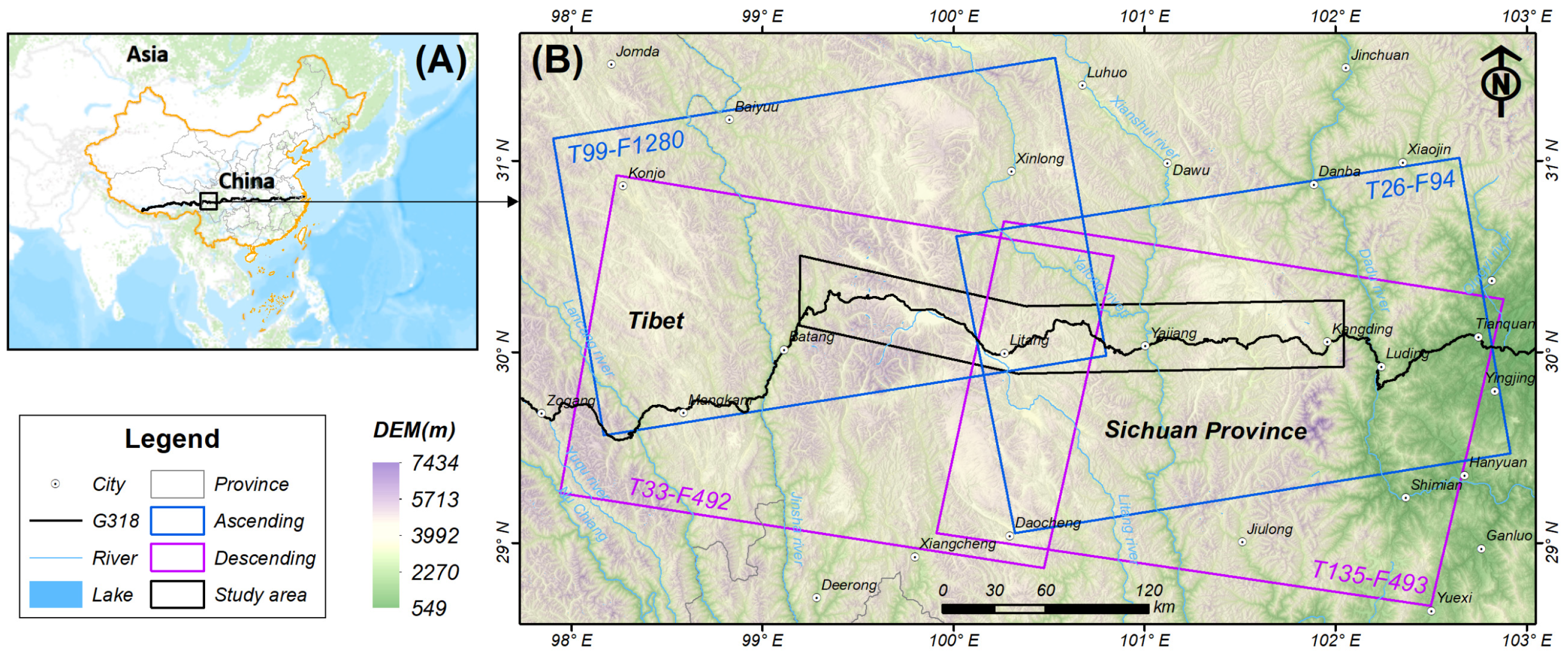
2.1. Study Area

From east to west, the G318 passes through Shanghai, Wuhan, Chongqing, Chengdu, and Lhasa. The Kangding-Batang section of the G318 is mainly located in Sichuan Province, and it is part of the Chengdu-Lhasa section. This study focuses on an area of 10,843 km2 along the Kangding-Batang section of the G318, which is seriously affected by landslide hazards, as shown in Figure 1.
The elevation of the study area varies greatly, being mostly above 2000 m, with the highest point over 5000 m, characterized by mountains and canyons. The study area belongs to the plateau climate zone, which is characterized by low temperature and rapid weather changes. From east to west, the rainfall in the study area gradually decreases, with an average annual rainfall of 700 mm. The river systems are very well developed, and several large rivers such as the Yalong River and Jinsha River pass through the study area. In addition, different types of modern glaciers have also developed in the alpine zone of the study area. Due to the high altitude, strong river/glacial erosion, and extreme climate change [44], the rocks in the study area are relatively fragmented and the slopes are steep, resulting in poor slope stability.
Geologically, the study area is located at the front edge of the Qinghai-Tibet Plateau, with strong tectonic movements. Some large active faults, such as the Xianshuihe fault and the Jinshajiang fault, have developed here. Historically, several large earthquakes (Ms > 7.0) have been recorded around the study area, such as the 1955 Ms 7.5 Kangding earthquake and the 1870 Ms 7.3 Batang earthquake. The stratigraphic lithology of the study area is very complex, with sandstone, conglomerate, and slate being the most developed. The Triassic and Permian are the most widely exposed strata.
Due to various factors, there are many types of landslide hazards in the study area. According to [47,48], we divided the landslides in the study area into the following categories: (1) slow-sliding rockslide; (2) debris flow, mainly the flow of various water-containing mixtures, e.g., a mixture of gravel, sand, and clay; (3) debris avalanche, mainly rock, ice, weathered materials, or a mixture falling, sliding, and accumulating. Since the study area has a high elevation with seasonal permafrost and glaciers, the flow of moraine cannot be ignored, and it has the potential to transform into glacial debris flows. Here, for the sake of simplicity, we classified landslides as debris flow or debris avalanche based on geomorphological criteria. Figure 2 presents several typical landslide photos from the Qinghai-Tibet Plateau.

2.2. Data

In this study, C-band Sentinel-1 Single Look Complex (SLC) images with the VV polarization mode were adopted for landslide mapping. Sentinel-1 data can be obtained from the Copernicus Open Access Hub or Alaska Satellite Facility for free, and a 12-day repeat acquisition allows us to conduct intensive ground object monitoring [40]. As shown in Figure 1, two ascending frames (Path 26, Frame 94 and Path 99, Frame 1280) and two descending frames (Path 135, Frame 493 and Path 33, Frame 492) can basically cover the whole study area. The detailed data used can be found in Table 1.
In addition, an SRTM digital elevation model (DEM) with a spatial resolution of 30 m was used in the data processing. Optical images with a resolution higher than 2 m (e.g., Google images and Tianditu images) were also adopted to classify and finalize landslide boundaries.

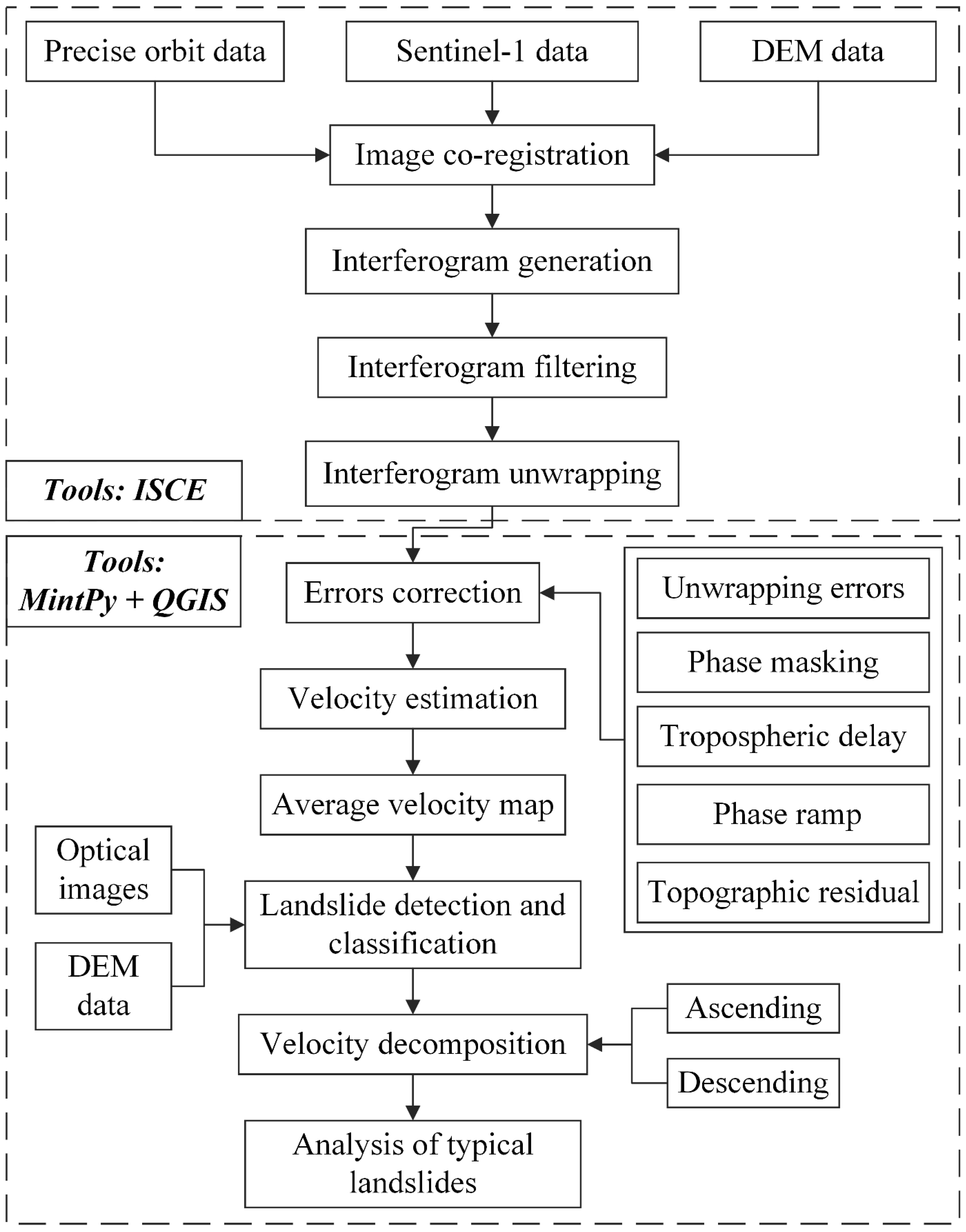
3. Time-Series InSAR Method

In this study, the time-series InSAR method was adopted to detect landslides in the study area. As shown in Figure 3, it consists of three main steps. First, the open-source InSAR Scientific Computer Environment (ISCE) tool (https://github.com/isce-framework/isce2, accessed on 25 February 2022) [49] was applied to generate unwrapped differential interferograms for the study area. We then used open-source Miami InSAR time-series software in the Python (MintPy) tool (https://github.com/insarlab/MintPy, accessed on 1 March 2022) [50] to correct the corresponding errors and perform the time-series analysis. Finally, open-source QGIS software was adopted to detect and identify landslides. The entire workflow is semi-automatic based on open-source tools or software, which provides a paradigm for landslide-related research in other mountainous regions of the world.
Specifically, we processed 324/326 differential interferometric pairs on the ascending track (P26 F94/P99 F1280) and 285/348 differential interferometric pairs on the descending track (P135 F493/P33 F492), respectively. These differential interferometric pairs were constructed using the Sentinel-1 stack processing chain [51], which is provided by the ISCE tool package. At the start of processing, all SLCs were co-registered to a single reference image. Each SLC was employed to generate interferometric pairs with the next three SLCs. The 30-m SRTM DEM was used to geocode these interferograms. In addition, the multi-look factor was set to 9:3, and the SNAPHU algorithm [52] was applied to unwrap the interferograms.
Before estimating the velocity, we needed to correct all kinds of errors using the open-source MintPy tool, mainly including phase unwrapping, tropospheric delay, phase ramps, and topographic residual [53]. Details about error correction can be found in [50]. In this study, bridging + phase closure method was applied to correct the phase unwrapping errors in the interferograms. Noise pixels with coherence of less than 0.4 were masked out. Generic Atmospheric Correction Online Service (GACOS) products were downloaded and adopted to correct the tropospheric delay [54,55]. We applied the quadratic polynomial to estimate and remove phase ramps that may be caused by residual tropospheric or ionospheric delays and orbital errors [50]. Since our aim is to carry out a semi-automatic InSAR processing strategy, we did not compare and analyze the effects of different processing algorithms and parameter settings.
Subsequently, we estimated the average deformation rates of the ascending and descending tracks, respectively, and obtained the corresponding line-of-sight (LOS) velocity maps and their standard deviation maps. Note that the standard deviation of velocity measures the uncertainty of the velocity field. The uncertainty of velocity needs to be considered in the analysis process. To reduce the uncertainty of the analysis, we therefore focused our analysis on those regions where the velocity was at least two times larger than its standard deviation [40]. In addition, considering that landslides do not occur in flat areas, we focused mainly on areas with a slope angle greater than 5 degrees. Based on average velocity maps, we adopted open-source QGIS software to visually interpret landslides in the study area. In the process of interpretation, high-resolution optical images and DEM data were also used to accurately classify and delineate the landslide boundaries.
The estimated average velocity is in the LOS direction, which is not conducive to analyzing the real sliding state of the slope. Thus, for typical landslides, velocity decomposition was performed in this study. Under the assumption that there is no deformation in the north–south (N–S) direction, we decomposed the vertical and horizontal (i.e., the east–west (E–W) direction) deformation components by combining the ascending and descending deformation information [56,57]. Assuming that the deformations in the vertical and horizontal directions are dv and dh, they can be deduced by the following equation [57,58].
d l o s = d v cos λ d h cos θ sin λ
where dlos, λ, and θ denote the deformation, radar incidence angle, and azimuth angle.

4. Results

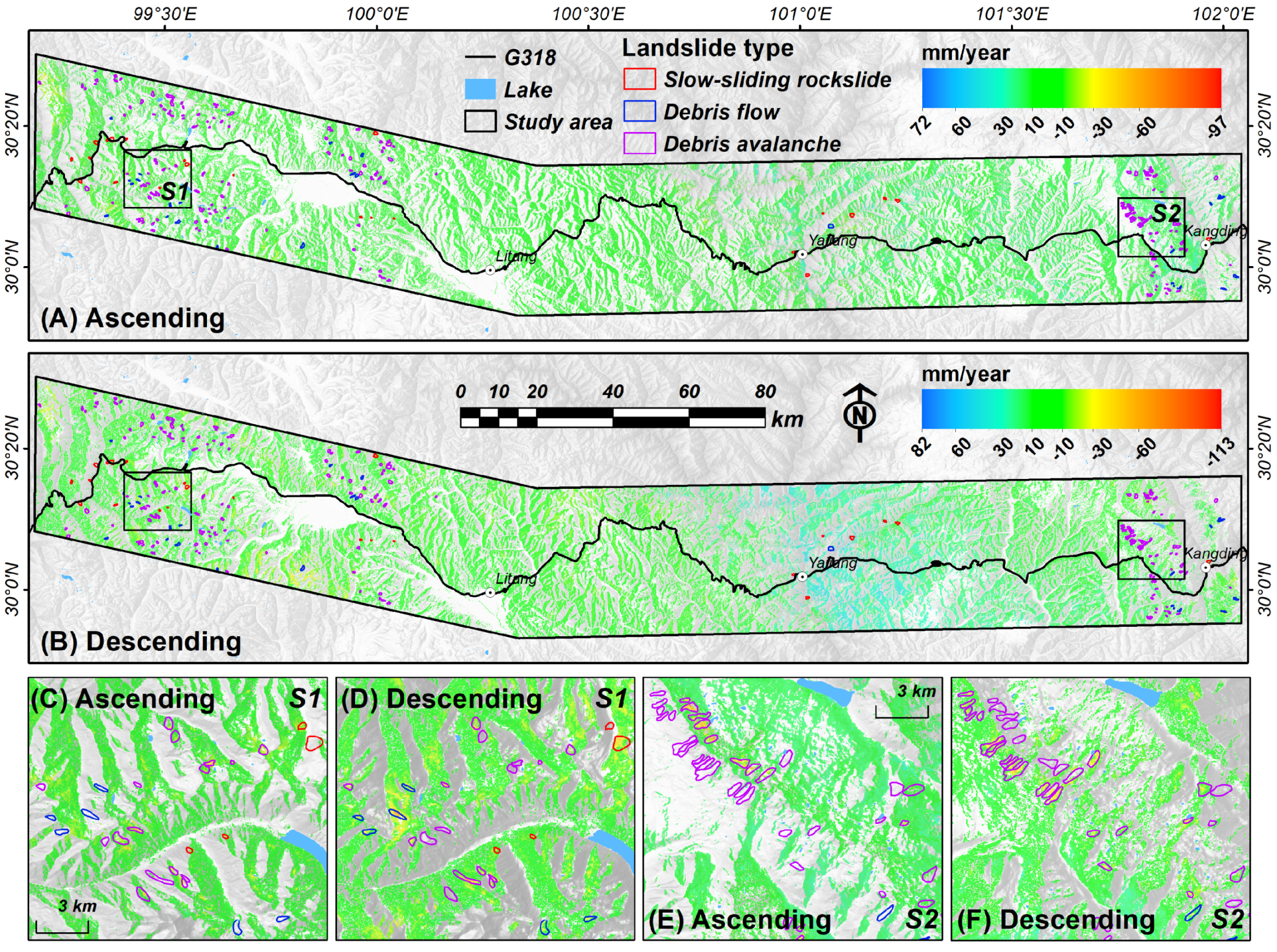
4.1. Annual Deformation Results

Figure 4 presents the annual LOS deformation results for the study area derived from the Sentinel-1 data (including ascending and descending). It should be noted that the positive value indicates the movement close to the satellite sensor and vice versa for the negative value. The average LOS deformation rate of the ascending track ranges from −97 to 72 mm/year, with a mean value of 3.74 mm/year. The average LOS deformation rate of the descending track ranges from −113 to 82 mm/year, with a mean value of 3.30 mm/year. The deformation trends derived from ascending and descending data are basically consistent. Although we adopted some error corrections during the estimation of the deformation rate, it can be seen that there are still some errors (e.g., topographic, atmospheric, and unwrapping errors) in the study area that have not been completely removed. Considering that our goal is to implement a semi-automatic InSAR processing strategy, we did not use additional methods for further removal of these residuals. Additionally, mountainous areas with high vegetation cover and steep terrain can lead to severe decorrelation (e.g., the Yajing section), and some regions with actual deformation may be masked and obscured due to the coherence mask processing (the threshold was set to 0.4). The deformation results in such areas may be noisy and uncertain. In this case, the interpretation of landslides in these areas requires great care to avoid misidentification.
In mountainous and vegetated areas, if the absolute value of LOS velocity is below 6–7 mm/year, the scatterers are corrupted by strong noise [59]. We, therefore, mainly analyzed the coherent target points with a deformation rate greater than 10 mm/year in this study. According to the ascending and descending deformation maps, we visually interpreted 236 potential landslides in total. Among them, 16 potential landslides (about 7%) were interpreted by both the ascending and descending results, and 86 (about 36%) and 134 (about 57%) potential landslides were interpreted by only the ascending or descending results, respectively. As shown in Figure 4, the spatial distribution of landslides is uneven, being mainly distributed in the Kangding section and the Litang to Batang section, while the middle Kangding to Litang section is relatively stable, with fewer landslides.

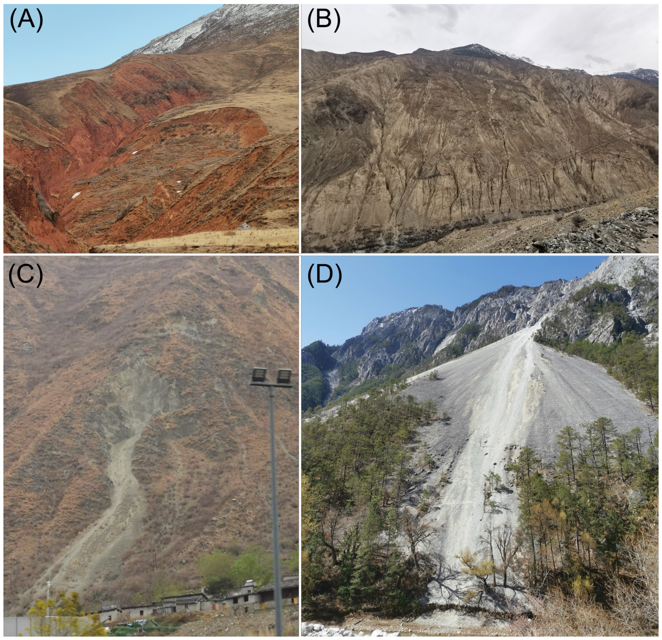
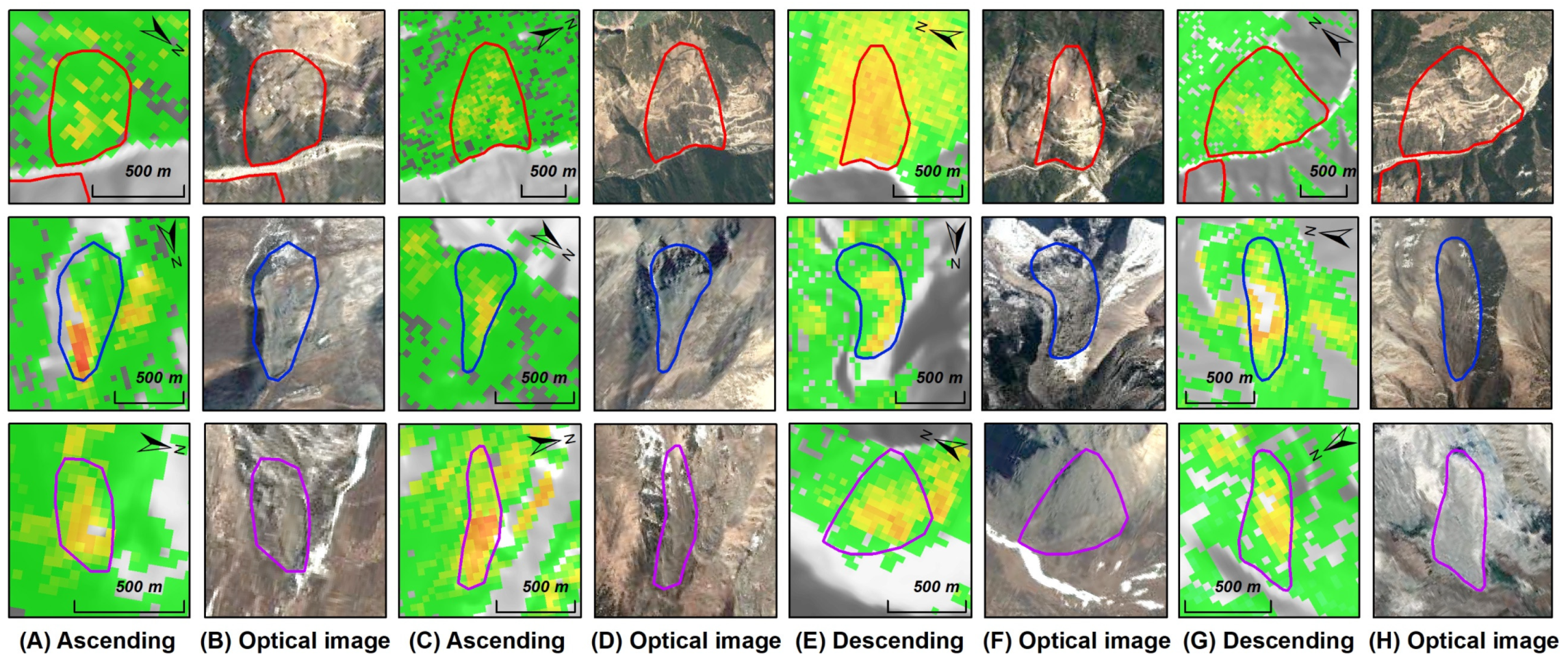
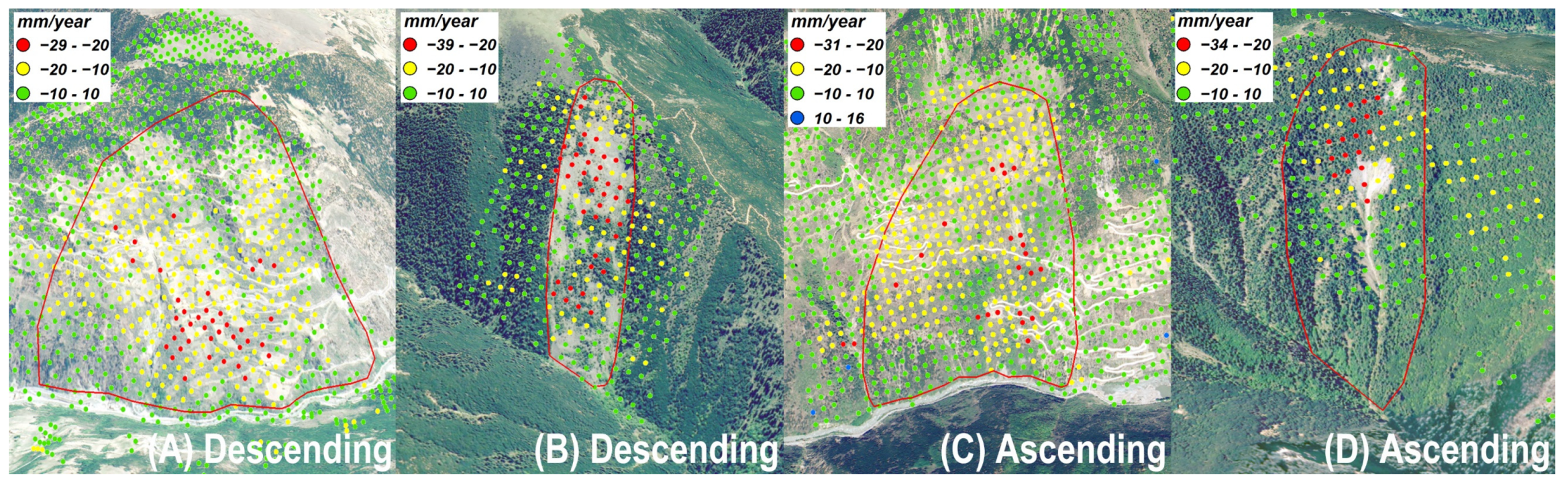
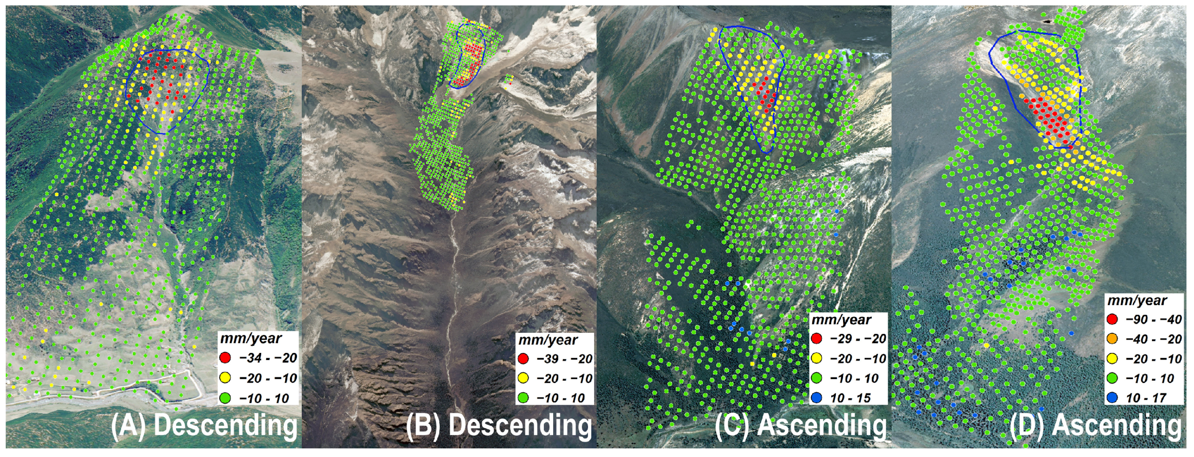
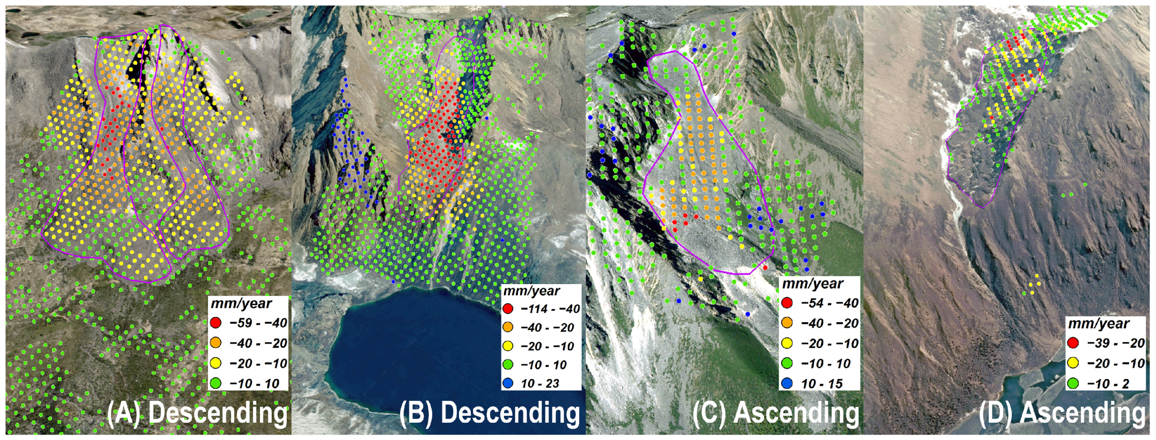
4.2. Landslide Detection and Classification

Based on the topographic features, optical image characteristics, and deformation rates, the identified potential landslides in the study area were manually classified into three categories, including 24 slow-sliding rockslides (10%), 30 debris flows (13%), and 182 debris avalanches (77%). Several typical potential landslides are shown in Figure 5.

4.2.1. Slow-Sliding Rockslides

As shown in Figure 6, the LOS deformation rate of most slow-sliding rockslides is 10~30 mm/year, and the maximum value of some coherent target points even reaches 39 mm/year. The deformation mainly occurs in the middle and top of the slope. It can be observed that these landslides have shape features such as chair or pear shape in the optical images, and some of them even clearly show crown cracks and minor scarp.
Of the 24 identified slow-sliding rockslides, the smallest landslide has an area of about 44,837 m2, the largest has 898,114 m2, and the average area reaches 351,139 m2. The identified landslides are generally large. The types of landslides mainly include old landslides and new ones triggered by human activities and natural factors. Geographically, they are mainly distributed on both sides of roads and rivers, and most may be affected by river erosion and road excavation. They are mainly composed of sandstone, limestone, and phyllite. Although the number of slow-sliding rockslides we identified is relatively small, their impact on the safety of the G318 should not be underestimated. Corresponding monitoring and prevention measures should be implemented to prevent future failure.

4.2.2. Debris Flows and Debris Avalanches

Due to the freezing weathering effect, high-altitude rocks are weathered, fractured, and disintegrated, thus forming loose debris accumulation in situ or nearby, which is characterized by large thickness, poor stability, and continuous distribution. Materially, the debris accumulation may be a mixture of various materials, such as rock, soil, and moraine deposits. From the optical images, we can also see obvious granular accumulation with rough texture features.
In the study area, we artificially classified such accumulations as debris flows and debris avalanches based on the hydrodynamic and topographic conditions, as they are important factors in triggering debris flow [60,61]. It should be noted that the identified debris flow is mainly the source of debris flow, not the entire debris flow area. As shown in Figure 4, debris flows and debris avalanches are quite common in the study area. The debris flows are mainly glacial debris flows recharged by glacial meltwater and rainy debris flows recharged by heavy rainfall. Their material sources are mostly located in high mountains, away from river valleys and roads. As shown in Figure 7, most of the coherent target points have deformation rates exceeding 30 mm/year, with the largest even exceeding 90 mm/year. The steep slope and long flow path make such debris flows very dangerous and difficult to monitor manually. Therefore, monitoring changes in the weather is essential for early warning of debris flows.
A total of 249 debris avalanches were identified in the study area, exceeding 70% of the total number of identifications. As shown in Figure 8, most of the coherent target points have deformation rates exceeding 30 mm/year, with the largest even exceeding 110 mm/year. Theoretically, the affected area of a debris avalanche is smaller than that of a debris flow. This is because it lacks sufficient hydrodynamic conditions or flow areas, although it has sufficient material sources. Normally, glacier meltwater is not enough to stimulate it, but it may evolve into slope debris flow under heavy rainfall.

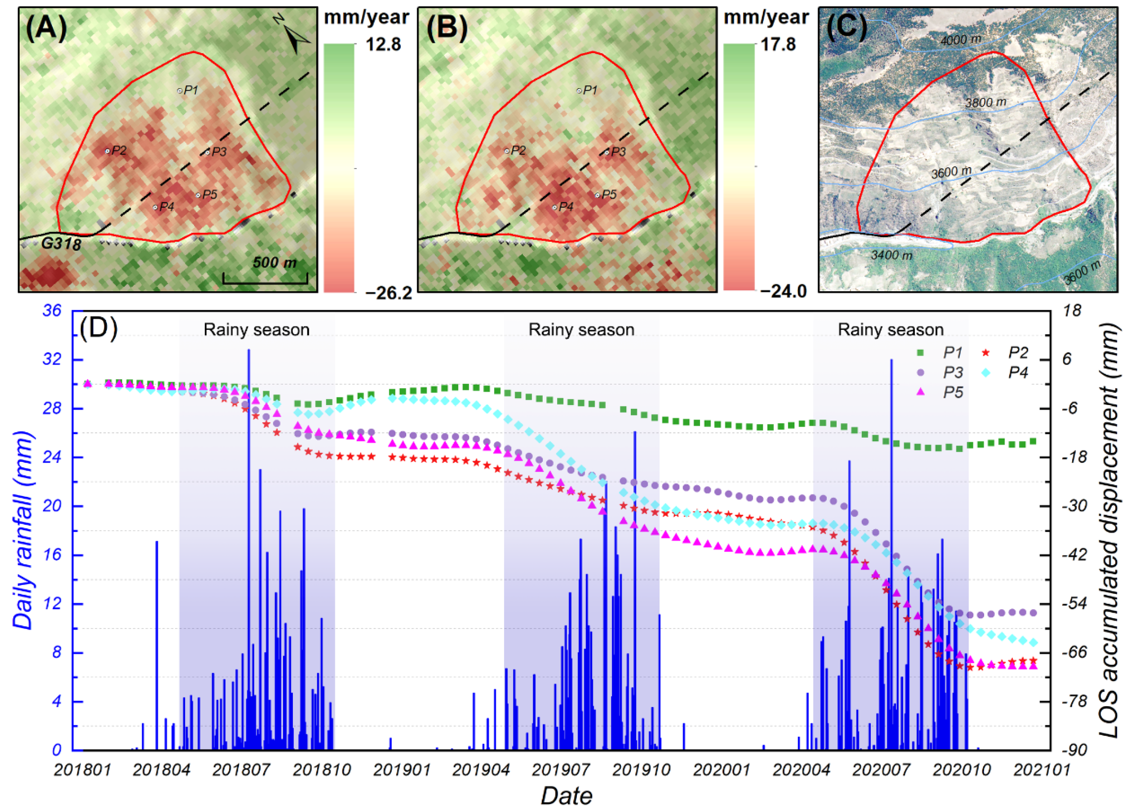
4.3. Analysis of a Typical Landslide

Due to the topography, most landslides in the study area can only be observed from a single satellite track (ascending or descending track). To quantitatively analyze the real deformation characteristics of the slope, we performed a deformation rate decomposition of one of the identified landslides, which can be observed from both the ascending and descending tracks. Results are shown in Figure 9.
For the vertical deformation rate, positive values indicate rising, while negative values indicate sinking. For the horizontal deformation rate, positive values indicate eastward movement, while negative values indicate westward movement. As shown in Figure 9A,B, both the vertical and horizontal deformation values of this slope are negative, indicating that this slope is subsiding in the vertical direction and moving westward in the horizontal direction. The deformation rates of this slope in the vertical and horizontal directions are comparable, with the maximum deformation rate reaching 20 mm/year. Considering that this slope is oriented to the southwest, it means that it may be a deep-seated gravitational landslide with very slow sliding. This landslide has a plane area of over 900,000 m2 and a vertical elevation difference of nearly 600 m. The G318 passes through the landslide in the form of a tunnel (the black dotted line in Figure 9A–C); however, some buildings can be found on the landslide from the optical images (Figure 9C). Thus, the threat of this landslide cannot be ignored. Moreover, some roads have been artificially excavated on the landslide, and these roads may have an impact on the stability of the landslide, which requires further attention in the future.
In addition, we analyzed the response of the accumulated deformation of several points on the landslide to the daily rainfall (Figure 9D). The rainy season in this area is from April to October. We observed a distinct pattern between landslide deformation and rainfall. Specifically, the landslide was relatively stable before July 2018, while during the period from July 2018 to October 2018 (rainy season), the middle and bottom of the landslide were in an accelerated sliding state. During the period from October 2018 to April 2019, the landslide was again in a relatively stable state due to little rainfall. Then, the landslide experienced significant accelerated sliding again in the 2019 rainy season. During this period, the LOS cumulative deformation at the middle and bottom of the landslide was significantly greater than that at the top of the landslide. The landslide was in a relatively stable state once again from October 2019 to April 2020, then significantly accelerated during the 2020 rainy season. The sliding parts are mainly the middle and bottom of the landslide, and the top of the landslide is relatively stable. Apparently, the rainfall has a significant triggering effect on the activity of the landslide. In general, the deformation state in the middle of the landslide needs to be closely monitored, as it is most likely to cause the failure of the entire landslide, especially during the rainy season.

5. Discussion

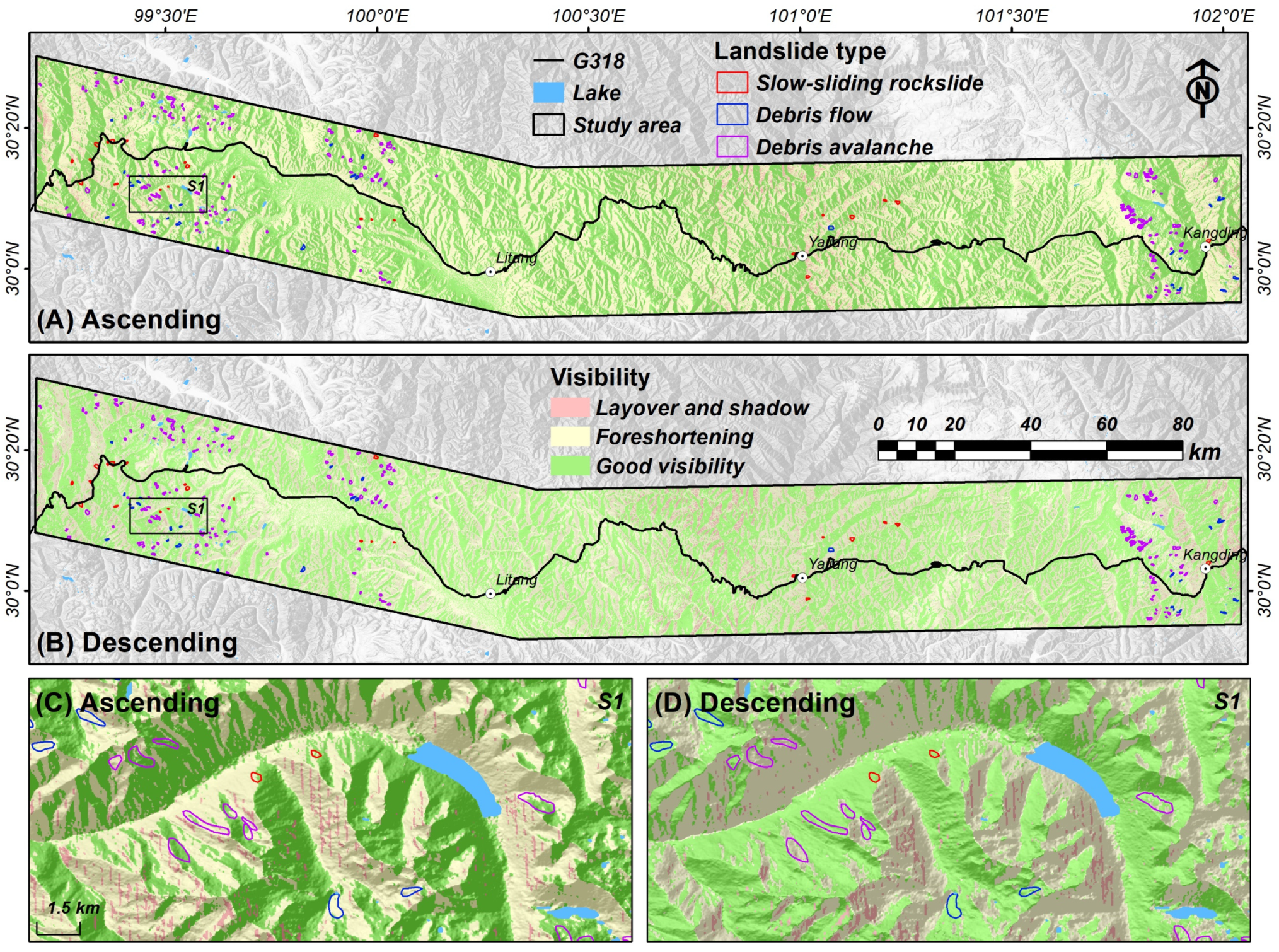
5.1. Analysis of Terrain Visibility

The study area has rugged terrain and large elevation changes, so it is necessary to analyze the visibility of SAR satellites. In this study, we adopted the R-index to measure the effect of topography [62]. The R-index measures the ratio between the radar slant range and the true ground range, and the detailed calculation formula and calculation steps can be found in [62,63].
As shown in Figure 10, we calculated the Sentinel-1 satellite geometric distortions over the entire study area and divided the study area into three categories: layover and shadow (bad visibility), foreshortening (medium visibility), and good visibility. The whole study area is severely affected by SAR geometric distortions. Quantitative statistical analysis shows that the good visibility areas of the ascending and descending tracks account for about 49.8% and 50.1% of the total area, respectively. Only 6% of the area is classified as a good visual area for both the ascending and descending tracks. This also explains the fact that most landslides (about 93%) were interpreted from a single orbit observation.
In addition, we found that for the ascending track (as shown in Figure 10A,C), the slopes facing west are mostly located in the satellite geometric distortion region, while the slopes facing east are located in the good visibility region, while the opposite is true for the descending track (as shown in Figure 10B,D). This is closely related to the SAR side-view imaging characteristics, as well as the incident direction of the SAR satellites. We further statistically found that about 99% of the study area can be observed by combining the ascending and descending data. Obviously, in mountainous areas, the combination of ascending and descending observation data can effectively reduce the effects of SAR geometric distortion and increase the observation area of satellite data.

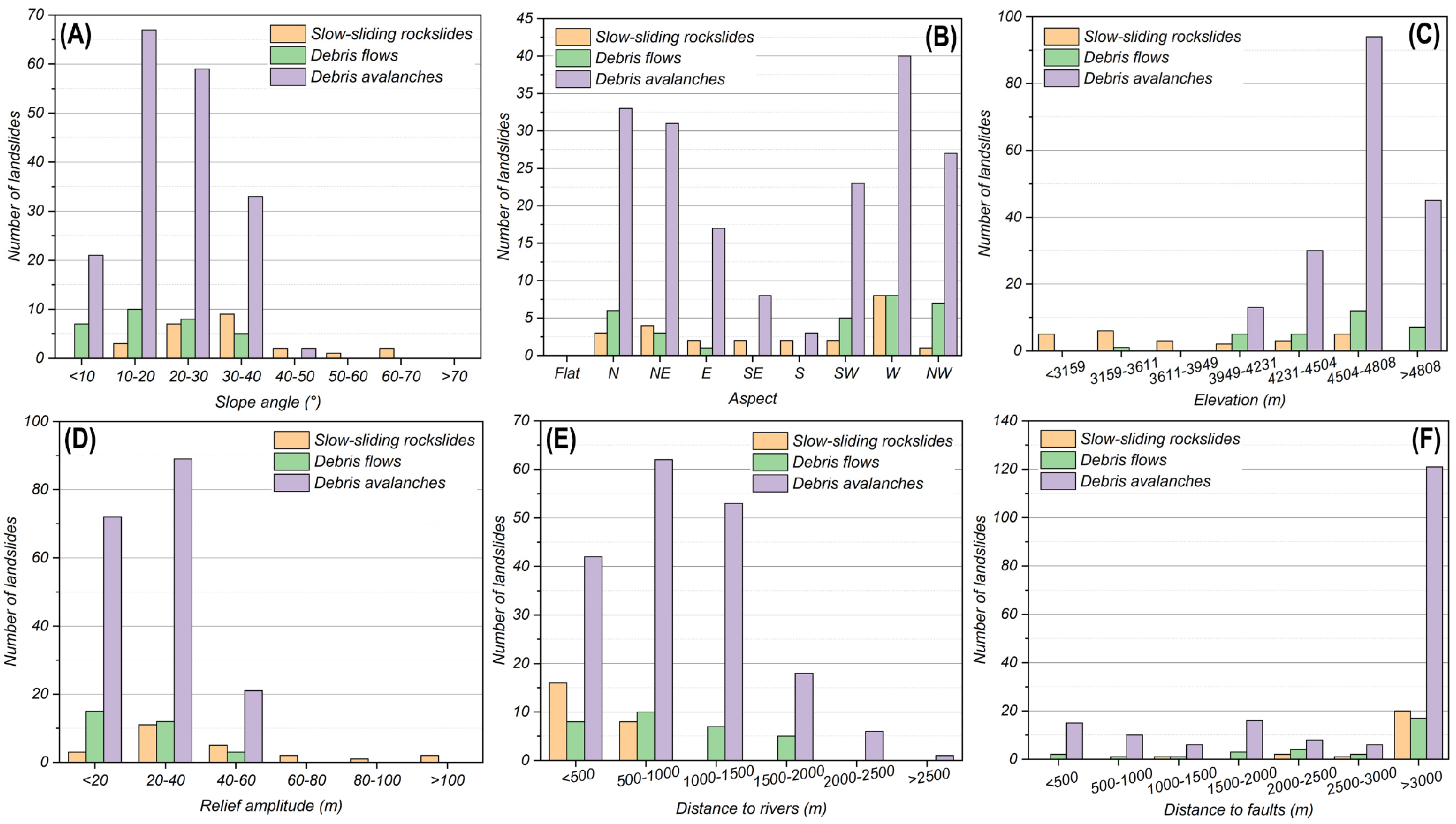
5.2. Factors Controlling Landslide Distribution

A landslide is a complex geographical phenomenon, closely related to various factors [64]. In this study, we briefly analyzed the relationship between landslides and several common controlling factors. The landslide controlling factors are shown in Figure 11.
As shown in Figure 12, it can be seen that most slow-moving rockslides occurred in relatively low-elevation areas (less than 4500 m), with slope angle mainly between 20° and 40°. In contrast, debris accumulations occurred in areas with higher elevation (greater than 3900 m) but gentler slope angle (less than 40°). In addition, we calculated the relief amplitude of the study area, which is defined as the difference between the maximum and minimum elevation values in the area (the 5 × 5 rectangle area was used in this study). We found that debris accumulations mainly occurred in areas with relief amplitude of less than 60 m, while slow-moving rockslides were sporadically distributed in areas with relief amplitude of greater than 60 m. This is generally in line with our understanding, as the gentle slope angle and topography ensure the rapid accumulation of this debris. In terms of the aspect, we found that most landslides occurred towards the north, northeast, and west directions, with few towards the south direction. Regarding the river factor, we found that slow-moving rockslides mainly occurred within 1000 m of rivers, and debris accumulations also had a relationship with rivers, i.e., the further away from rivers, the lower the number of debris accumulations. However, for faults, no obvious interrelationships were observed, and most landslides occurred 3000 m away from faults. In general, the topography of this area has a clear role in controlling the distribution of landslides.

5.3. Limitations and Future Recommendations

In this study, we adopted a semi-automated InSAR processing method to identify wide-area landslides. This method is implemented based on open-source tools or software and is highly efficient. Although there are still some unexplained errors in InSAR-derived deformation, the impact on large-area landslide detection is negligible. However, if this method is used to monitor an individual landslide, further adjustment of the inversion parameters and elimination of corresponding errors are required.
Although we identified a total of 236 landslides in this study, this is likely to be an underestimation. This is because a SAR satellite is insensitive to the deformation parallel to the satellite’s flight direction (near north–south), implying that landslides in this direction may have been omitted. Moreover, fast landslide movement can result in InSAR decorrelation (loss of coherence) and thus omission. Some factors such as SAR geometry distortions, vegetation cover, and steep terrain can also affect landslide identification. From this perspective, combining with other methods (such as LiDAR-based and field-based) to compensate and validate landslide results should be the focus of future work. In addition, we are not able to classify landslide types directly from the InSAR-derived surface deformation. Thus, optical images and a DEM are required to classify these landslides. In this study, the identified landslides were classified into only three categories, according to [47]. Due to the complexity of landslides, it is difficult to guarantee that each landslide has been correctly classified. However, from an application point of view, occasional misclassifications have little impact on engineering applications because each identified landslide needs to be carefully verified and checked in practice. From this point of view, field work is essential, and our identification results can effectively narrow the scope of field work. Therefore, the next step is to conduct field work to further validate the classification results.
InSAR observations are a combination of Earth surface motion, atmospheric changes, and measurement and processing errors [53]. In the Qinghai–Tibet Plateau region, permafrost freeze–thaw processes have been identified as an important source of surface deformation [27], especially under climate warming. In addition, tectonic processes also contribute to the deformation observed by InSAR. However, it is difficult to isolate such deformation sources from the InSAR-derived surface deformation. To be more specific, the deformation map used to detect landslides in this study may, to some extent, encompass other sources of deformation in addition to slope movement, implying that the landslide deformations we mapped may be biased. However, it is worth noting that most of the permafrost in the study area is seasonal, and the magnitudes of such deformations are ordinarily small. Moreover, seasonal permafrost deformation usually occurs in flat areas with a slope angle of less than 5 degrees, and decreases dramatically with increasing slope angle [27]. Obviously, the slope angle of our identification area is greater than 5 degrees, effectively avoiding the areas most affected by seasonal permafrost. In addition, surface deformation from tectonic movements is usually on the millimeter scale and therefore negligible in this study. In other words, large-scale surface deformation due to permafrost freeze–thaw processes and tectonic movement has essentially no effect on landslide identification in this study.

6. Conclusions

In this study, a semi-automated InSAR processing method was adopted to detect and analyze landslides along the Kangding-Batang section of Shanghai-Nyalam Road. A total of 446 ascending and descending Sentinel-1 images acquired from January 2018 to December 2021 were used, and 1283 interferograms were thus processed by using the open-source ISCE tool. In order to obtain relatively pure surface deformation rates, we used the open-source MintPy tool to perform a series of error corrections, such as tropospheric delay correction using GACOS data. Finally, 236 potential landslides were visually interpreted by combining deformation maps, optical images, and DEM data. According to topographic features, we manually classified these landslides into three categories, including 24 slow-sliding rockslides, 30 debris flows, and 182 debris avalanches. Among them, most landslides were only identified from a single satellite track, and only about 7% of landslides were identified from both the ascending and descending tracks. Considering the effect of SAR satellite geometric distortions, joint observations of ascending and descending tracks in mountainous areas are recommended, which can effectively reduce omissions. In addition, we performed deformation rate decomposition on a typical landslide to quantify its actual deformation characteristics, and we analyzed the relationship between its deformation and rainfall. Results showed that rainfall has a significant triggering effect on the landslide activity, and the deformation in the middle of the landslide needs close attention.
Understanding the distribution of landslides is essential for assessing the potential risk of landslides. Although InSAR technology can monitor the subtle deformation of slopes, due to the complexity of slopes, the true stability state of slopes still needs to be determined in combination with site investigation and on-site monitoring instruments. From this perspective, InSAR technology can effectively narrow the study area and provide targets for field investigation. Therefore, in the future, we will carry out field investigation to evaluate the identified landslides on a case-by-case basis.

Author Contributions

Conceptualization, Y.Y. and X.X.; methodology, Y.Y. and G.X.; software, Y.Y. and G.X.; validation, Y.Y. and H.G.; formal analysis, Y.Y.; investigation, H.G.; resources, Y.Y.; data curation, Y.Y.; writing—original draft preparation, Y.Y.; writing—review and editing, G.X. and H.G.; visualization, Y.Y.; supervision, X.X.; project administration, Y.Y.; funding acquisition, X.X. All authors have read and agreed to the published version of the manuscript.

Funding

This research was funded by the National Natural Science Foundation of China (grant numbers 41941016, U1839204, U2139201, 41572193, and 42104008) and the National Institute of Natural Hazards, Ministry of Emergency Management of China Research Fund (ZDJ2018-22).

Data Availability Statement

Not applicable.

Acknowledgments

Sentinel-1 SAR data can be downloaded from Copernicus Open Access Hub (https://scihub.copernicus.eu/, accessed on 18 February 2022), and GACOS products can be accessed from the website (http://www.gacos.net/, accessed on 19 May 2022). We appreciate the facility support provided by Ren Junjie.

Conflicts of Interest

The authors declare no conflict of interest.

References

  1. Lin, Q.; Wang, Y. Spatial and temporal analysis of a fatal landslide inventory in China from 1950 to 2016. Landslides 2018, 15, 2357–2372. [Google Scholar] [CrossRef]
  2. Lacroix, P.; Handwerger, A.L.; Bièvre, G. Life and death of slow-moving landslides. Nat. Rev. Earth Environ. 2020, 1, 404–419. [Google Scholar] [CrossRef]
  3. Dille, A.; Dewitte, O.; Handwerger, A.L.; d’Oreye, N.; Derauw, D.; Ganza Bamulezi, G.; Ilombe Mawe, G.; Michellier, C.; Moeyersons, J.; Monsieurs, E.; et al. Acceleration of a large deep-seated tropical landslide due to urbanization feedbacks. Nat. Geosci. 2022, 15, 1048–1055. [Google Scholar] [CrossRef]
  4. Emberson, R.; Kirschbaum, D.; Stanley, T. Global connections between El Nino and landslide impacts. Nat. Commun. 2021, 12, 2262. [Google Scholar] [CrossRef] [PubMed]
  5. LaHusen, S.R.; Duvall, A.R.; Booth, A.M.; Grant, A.; Mishkin, B.A.; Montgomery, D.R.; Struble, W.; Roering, J.J.; Wartman, J. Rainfall triggers more deep-seated landslides than Cascadia earthquakes in the Oregon Coast Range, USA. Sci. Adv. 2020, 6, eaba6790. [Google Scholar] [CrossRef]
  6. Petley, D. Global patterns of loss of life from landslides. Geology 2012, 40, 927–930. [Google Scholar] [CrossRef]
  7. Li, W.; Zhan, W.; Lu, H.; Xu, Q.; Pei, X.; Wang, D.; Huang, R.; Ge, D. Precursors to large rockslides visible on optical remote-sensing images and their implications for landslide early detection. Landslides 2022, 20, 1–12. [Google Scholar] [CrossRef]
  8. Xu, C. Preparation of earthquake-triggered landslide inventory maps using remote sensing and GIS technologies: Principles and case studies. Geosci. Front. 2015, 6, 825–836. [Google Scholar] [CrossRef] [Green Version]
  9. Fiorucci, F.; Ardizzone, F.; Mondini, A.C.; Viero, A.; Guzzetti, F. Visual interpretation of stereoscopic NDVI satellite images to map rainfall-induced landslides. Landslides 2018, 16, 165–174. [Google Scholar] [CrossRef]
  10. Sato, H.P.; Harp, E.L. Interpretation of earthquake-induced landslides triggered by the 12 May 2008, M7.9 Wenchuan earthquake in the Beichuan area, Sichuan Province, China using satellite imagery and Google Earth. Landslides 2009, 6, 153–159. [Google Scholar] [CrossRef]
  11. Lu, P.; Qin, Y.; Li, Z.; Mondini, A.C.; Casagli, N. Landslide mapping from multi-sensor data through improved change detection-based Markov random field. Remote Sens. Environ. 2019, 231, 111235. [Google Scholar] [CrossRef]
  12. Ramos-Bernal, N.R.; Vázquez-Jiménez, R.; Romero-Calcerrada, R.; Arrogante-Funes, P.; Novillo, J.C. Evaluation of Unsupervised Change Detection Methods Applied to Landslide Inventory Mapping Using ASTER Imagery. Remote Sens. 2018, 10, 1987. [Google Scholar] [CrossRef] [Green Version]
  13. Qu, F.; Qiu, H.; Sun, H.; Tang, M. Post-failure landslide change detection and analysis using optical satellite Sentinel-2 images. Landslides 2020, 18, 447–455. [Google Scholar] [CrossRef]
  14. Martha, T.R.; Kerle, N.; van Westen, C.J.; Jetten, V.; Vinod Kumar, K. Object-oriented analysis of multi-temporal panchromatic images for creation of historical landslide inventories. ISPRS J. Photogramm. Remote Sens. 2012, 67, 105–119. [Google Scholar] [CrossRef]
  15. Feizizadeh, B.; Blaschke, T.; Tiede, D.; Moghaddam, M.H.R. Evaluating fuzzy operators of an object-based image analysis for detecting landslides and their changes. Geomorphology 2017, 293, 240–254. [Google Scholar] [CrossRef]
  16. Amatya, P.; Kirschbaum, D.; Stanley, T.; Tanyas, H. Landslide mapping using object-based image analysis and open source tools. Eng. Geol. 2021, 282, 106000. [Google Scholar] [CrossRef]
  17. Meena, S.R.; Soares, L.P.; Grohmann, C.H.; van Westen, C.; Bhuyan, K.; Singh, R.P.; Floris, M.; Catani, F. Landslide detection in the Himalayas using machine learning algorithms and U-Net. Landslides 2022, 19, 1209–1229. [Google Scholar] [CrossRef]
  18. Yi, Y.; Zhang, W. A New Deep-Learning-Based Approach for Earthquake-Triggered Landslide Detection From Single-Temporal RapidEye Satellite Imagery. IEEE J. Sel. Top. Appl. Earth Obs. Remote Sens. 2020, 13, 6166–6176. [Google Scholar] [CrossRef]
  19. Shi, W.; Zhang, M.; Ke, H.; Fang, X.; Zhan, Z.; Chen, S. Landslide Recognition by Deep Convolutional Neural Network and Change Detection. IEEE Trans. Geosci. Remote Sens. 2020, 59, 1–19. [Google Scholar] [CrossRef]
  20. Liu, T.; Chen, T.; Niu, R.; Plaza, A. Landslide Detection Mapping Employing CNN, ResNet, and DenseNet in the Three Gorges Reservoir, China. IEEE J. Sel. Top. Appl. Earth Obs. Remote Sens. 2021, 14, 11417–11428. [Google Scholar] [CrossRef]
  21. Mondini, A.C.; Guzzetti, F.; Reichenbach, P.; Rossi, M.; Cardinali, M.; Ardizzone, F. Semi-automatic recognition and mapping of rainfall induced shallow landslides using optical satellite images. Remote Sens. Environ. 2011, 115, 1743–1757. [Google Scholar] [CrossRef]
  22. Xu, Q. Understanding and Consideration of Related Issues in Early Identification of Potential Geohazards. Geomat. Inf. Sci. Wuhan Univ. 2020, 45, 1651–1659. [Google Scholar]
  23. Ren, T.; Gong, W.; Bowa, V.M.; Tang, H.; Chen, J.; Zhao, F. An Improved R-Index Model for Terrain Visibility Analysis for Landslide Monitoring with InSAR. Remote Sens. 2021, 13, 1938. [Google Scholar] [CrossRef]
  24. Zhu, J.; Li, Z.; Hu, J. Research Progress and Methods of InSAR for Deformation Monitoring. Acta Geod. Et Cartogr. Sin. 2017, 46, 1717–1733. [Google Scholar]
  25. Parizzi, A.; Brcic, R.; De Zan, F. InSAR Performance for Large-Scale Deformation Measurement. IEEE Trans. Geosci. Remote Sens. 2021, 59, 8510–8520. [Google Scholar] [CrossRef]
  26. Wang, Y.; Dong, J.; Zhang, L.; Zhang, L.; Deng, S.; Zhang, G.; Liao, M.; Gong, J. Refined InSAR tropospheric delay correction for wide-area landslide identification and monitoring. Remote Sens. Environ. 2022, 275, 113013. [Google Scholar] [CrossRef]
  27. Chen, J.; Wu, T.; Zou, D.; Liu, L.; Wu, X.; Gong, W.; Zhu, X.; Li, R.; Hao, J.; Hu, G.; et al. Magnitudes and patterns of large-scale permafrost ground deformation revealed by Sentinel-1 InSAR on the central Qinghai-Tibet Plateau. Remote Sens. Environ. 2022, 268, 112778. [Google Scholar] [CrossRef]
  28. Hooper, A.; Bekaert, D.; Spaans, K.; Arıkan, M. Recent advances in SAR interferometry time series analysis for measuring crustal deformation. Tectonophysics 2012, 514–517, 1–13. [Google Scholar] [CrossRef]
  29. ElGharbawi, T.; Tamura, M. Coseismic and postseismic deformation estimation of the 2011 Tohoku earthquake in Kanto Region, Japan, using InSAR time series analysis and GPS. Remote Sens. Environ. 2015, 168, 374–387. [Google Scholar] [CrossRef] [Green Version]
  30. Gabriel, A.K.; Goldstein, R.M.; Zebker, H.A. Mapping small elevation changes over large areas: Differential radar interferometry. J. Geophys. Res. 1989, 94, 9183–9191. [Google Scholar] [CrossRef]
  31. Crosetto, M.; Monserrat, O.; Cuevas-González, M.; Devanthéry, N.; Crippa, B. Persistent Scatterer Interferometry: A review. ISPRS J. Photogramm. Remote Sens. 2016, 115, 78–89. [Google Scholar] [CrossRef] [Green Version]
  32. Ferretti, A.; Prati, C.; Rocca, F. Permanent scatterers in SAR interferometry. IEEE Trans. Geosci. Remote Sens. 2001, 39, 8–20. [Google Scholar] [CrossRef]
  33. Berardino, P.; Fornaro, G.; Lanari, R.; Sansosti, E. A new algorithm for surface deformation monitoring based on small baseline differential SAR interferograms. IEEE Trans. Geosci. Remote Sens. 2002, 40, 2375–2383. [Google Scholar] [CrossRef] [Green Version]
  34. Li, S.; Xu, W.; Li, Z. Review of the SBAS InSAR Time-series algorithms, applications, and challenges. Geod. Geodyn. 2022, 13, 114–126. [Google Scholar] [CrossRef]
  35. Dong, J.; Liao, M.; Xu, Q.; Zhang, L.; Tang, M.; Gong, J. Detection and displacement characterization of landslides using multi-temporal satellite SAR interferometry: A case study of Danba County in the Dadu River Basin. Eng. Geol. 2018, 240, 95–109. [Google Scholar] [CrossRef]
  36. Pourkhosravani, M.; Mehrabi, A.; Pirasteh, S.; Derakhshani, R. Monitoring of Maskun landslide and determining its quantitative relationship to different climatic conditions using D-InSAR and PSI techniques. Geomat. Nat. Hazards Risk 2022, 13, 1134–1153. [Google Scholar] [CrossRef]
  37. Lu, P.; Casagli, N.; Catani, F.; Tofani, V. Persistent Scatterers Interferometry Hotspot and Cluster Analysis (PSI-HCA) for detection of extremely slow-moving landslides. Int. J. Remote Sens. 2011, 33, 466–489. [Google Scholar] [CrossRef]
  38. Carla, T.; Intrieri, E.; Raspini, F.; Bardi, F.; Farina, P.; Ferretti, A.; Colombo, D.; Novali, F.; Casagli, N. Perspectives on the prediction of catastrophic slope failures from satellite InSAR. Sci. Rep. 2019, 9, 14137. [Google Scholar] [CrossRef] [Green Version]
  39. Eriksen, H.Ø.; Lauknes, T.R.; Larsen, Y.; Corner, G.D.; Bergh, S.G.; Dehls, J.; Kierulf, H.P. Visualizing and interpreting surface displacement patterns on unstable slopes using multi-geometry satellite SAR interferometry (2D InSAR). Remote Sens. Environ. 2017, 191, 297–312. [Google Scholar] [CrossRef] [Green Version]
  40. Bekaert, D.P.S.; Handwerger, A.L.; Agram, P.; Kirschbaum, D.B. InSAR-based detection method for mapping and monitoring slow-moving landslides in remote regions with steep and mountainous terrain: An application to Nepal. Remote Sens. Environ. 2020, 249, 111983. [Google Scholar] [CrossRef]
  41. Zhang, L.; Dai, K.; Deng, J.; Ge, D.; Liang, R.; Li, W.; Xu, Q. Identifying Potential Landslides by Stacking-InSAR in Southwestern China and Its Performance Comparison with SBAS-InSAR. Remote Sens. 2021, 13, 3662. [Google Scholar] [CrossRef]
  42. Zhao, C.; Lu, Z.; Zhang, Q.; de la Fuente, J. Large-area landslide detection and monitoring with ALOS/PALSAR imagery data over Northern California and Southern Oregon, USA. Remote Sens. Environ. 2012, 124, 348–359. [Google Scholar] [CrossRef]
  43. Jiang, G.; Xu, C.; Wen, Y.; Xu, X.; Ding, K.; Wang, J. Contemporary tectonic stressing rates of major strike-slip faults in the Tibetan Plateau from GPS observations using Least-Squares Collocation. Tectonophysics 2014, 615–616, 85–95. [Google Scholar] [CrossRef]
  44. Cui, P.; Ge, Y.; Li, S.; Li, Z.; Xu, X.; Zhou, G.G.D.; Chen, H.; Wang, H.; Lei, Y.; Zhou, L.; et al. Scientific challenges in disaster risk reduction for the Sichuan–Tibet Railway. Eng. Geol. 2022, 309, 106837. [Google Scholar] [CrossRef]
  45. Shi, X.; Jiang, L.; Jiang, H.; Wang, X.; Xu, J. Geohazards Analysis of the Litang–Batang Section of Sichuan–Tibet Railway Using SAR Interferometry. IEEE J. Sel. Top. Appl. Earth Obs. Remote Sens. 2021, 14, 11998–12006. [Google Scholar] [CrossRef]
  46. Zhang, J.; Zhu, W.; Cheng, Y.; Li, Z. Landslide Detection in the Linzhi–Ya’an Section along the Sichuan–Tibet Railway Based on InSAR and Hot Spot Analysis Methods. Remote Sens. 2021, 13, 3566. [Google Scholar] [CrossRef]
  47. Hungr, O.; Leroueil, S.; Picarelli, L. The Varnes classification of landslide types, an update. Landslides 2014, 11, 167–194. [Google Scholar] [CrossRef]
  48. Varnes, D.J. Slope movement types and processes, Landslides: Analyses and Control. Trans. Res. Bd. Spec. Rep. 1978, 176, 11–33. [Google Scholar]
  49. Rosen, P.A.; Gurrola, E.; Sacco, G.F.; Zebker, H. The InSAR scientific computing environment. In Proceedings of the EUSAR 2012; 9th European Conference on Synthetic Aperture Radar, Nuremberg, Germany, 23–26 April 2012; pp. 730–733. [Google Scholar]
  50. Yunjun, Z.; Fattahi, H.; Amelung, F. Small baseline InSAR time series analysis: Unwrapping error correction and noise reduction. Comput. Geosci. 2019, 133, 104331. [Google Scholar] [CrossRef] [Green Version]
  51. Fattahi, H.; Agram, P.; Simons, M. A Network-Based Enhanced Spectral Diversity Approach for TOPS Time-Series Analysis. IEEE Trans. Geosci. Remote Sens. 2017, 55, 777–786. [Google Scholar] [CrossRef] [Green Version]
  52. Chen, C.W.; Zebker, H.A. Phase unwrapping for large SAR interferograms: Statistical segmentation and generalized network models. IEEE Trans. Geosci. Remote Sens. 2002, 40, 1709–1719. [Google Scholar] [CrossRef] [Green Version]
  53. Stephenson, O.L.; Liu, Y.K.; Yunjun, Z.; Simons, M.; Rosen, P.; Xu, X. The Impact of Plate Motions on Long-Wavelength InSAR-Derived Velocity Fields. Geophys. Res. Lett. 2022, 49. [Google Scholar] [CrossRef]
  54. Yu, C.; Li, Z.; Penna, N.T. Interferometric synthetic aperture radar atmospheric correction using a GPS-based iterative tropospheric decomposition model. Remote Sens. Environ. 2018, 204, 109–121. [Google Scholar] [CrossRef]
  55. Yu, C.; Li, Z.; Penna, N.T.; Crippa, P. Generic Atmospheric Correction Model for Interferometric Synthetic Aperture Radar Observations. J. Geophys. Res. Solid Earth 2018, 123, 9202–9222. [Google Scholar] [CrossRef]
  56. Fialko, Y.; Simons, M.; Agnew, D. The complete (3-D) surface displacement field in the epicentral area of the 1999MW7.1 Hector Mine Earthquake, California, from space geodetic observations. Geophys. Res. Lett. 2001, 28, 3063–3066. [Google Scholar] [CrossRef] [Green Version]
  57. Wright, T.J. Toward mapping surface deformation in three dimensions using InSAR. Geophys. Res. Lett. 2004, 31. [Google Scholar] [CrossRef] [Green Version]
  58. Zhang, T.; Zhang, W.; Cao, D.; Yi, Y.; Wu, X. A New Deep Learning Neural Network Model for the Identification of InSAR Anomalous Deformation Areas. Remote Sens. 2022, 14, 2690. [Google Scholar] [CrossRef]
  59. Kovács, I.P.; Bugya, T.; Czigány, S.; Defilippi, M.; Lóczy, D.; Riccardi, P.; Ronczyk, L.; Pasquali, P. How to avoid false interpretations of Sentinel-1A TOPSAR interferometric data in landslide mapping? A case study: Recent landslides in Transdanubia, Hungary. Nat. Hazards 2018, 96, 693–712. [Google Scholar] [CrossRef] [Green Version]
  60. Pastorello, R.; D’Agostino, V.; Hürlimann, M. Debris flow triggering characterization through a comparative analysis among different mountain catchments. Catena 2020, 186, 104348. [Google Scholar] [CrossRef]
  61. Zou, Q.; Zhou, G.G.D.; Li, S.; Ouyang, C.; Tang, J. Dynamic Process Analysis and Hazard Prediction of Debris Flow in Eastern Qinghai-Tibet Plateau Area—A Case Study at Ridi Gully. Arct. Antarct. Alp. Res. 2018, 49, 373–390. [Google Scholar] [CrossRef] [Green Version]
  62. Notti, D.; Herrera, G.; Bianchini, S.; Meisina, C.; García-Davalillo, J.C.; Zucca, F. A methodology for improving landslide PSI data analysis. Int. J. Remote Sens. 2014, 35, 2186–2214. [Google Scholar] [CrossRef]
  63. Cigna, F.; Bateson, L.B.; Jordan, C.J.; Dashwood, C. Simulating SAR geometric distortions and predicting Persistent Scatterer densities for ERS-1/2 and ENVISAT C-band SAR and InSAR applications: Nationwide feasibility assessment to monitor the landmass of Great Britain with SAR imagery. Remote Sens. Environ. 2014, 152, 441–466. [Google Scholar] [CrossRef] [Green Version]
  64. Yi, Y.; Zhang, W.; Xu, X.; Zhang, Z.; Wu, X. Evaluation of neural network models for landslide susceptibility assessment. Int. J. Digit. Earth 2022, 15, 934–953. [Google Scholar] [CrossRef]
Figure 1. Overview of the study area. (A) Location of the G318 and the study area; (B) topographic map of the study area. The purple and blue rectangles outline the coverage of the Sentinel-1 SAR images. The black polygon shows the extent of the study area.
Remotesensing 15 01452 g001
Figure 2. Photos of several typical landslides taken during field investigation: (A) shallow soil sliding; (B) old rockslide; (C) rock fall; (D) debris falling, sliding, and accumulating.
Remotesensing 15 01452 g002
Figure 3. Workflow of this study.
Remotesensing 15 01452 g003
Figure 4. Results of deformation and landslide identification in the study area: (A) ascending, (B) descending, (CF) enlarged maps of subregions. The base map is the hillshade data calculated from the DEM.
Remotesensing 15 01452 g004
Figure 5. Typical landslide deformation maps and optical images. The optical images (about 2-m resolution) were obtained from the Google Earth platform. (The legend is the same as Figure 4.)
Remotesensing 15 01452 g005
Figure 6. LOS velocity of typical slow-sliding rockslides. The base map is the Tianditu images with a spatial resolution of 1 m. The red line represents the boundary of slow-sliding rockslides.
Remotesensing 15 01452 g006
Figure 7. LOS velocity of typical debris flows. The base map is the Tianditu images with a spatial resolution of 1 m. The blue line represents the boundary of debris flows.
Remotesensing 15 01452 g007
Figure 8. LOS velocity of typical debris avalanches. The base map is the Tianditu images with a spatial resolution of 1 m. The purple line represents the boundary of debris avalanches.
Remotesensing 15 01452 g008
Figure 9. Landslide monitoring and analysis. (A,B) Vertical and horizontal deformation rate maps. The red line represents the landslide boundary, and the black dotted line represents the tunnel. (C) Tianditu image with a spatial resolution of 1 m. The blue lines represent the contour lines of the area. (D) LOS displacements of several points versus daily rainfall.
Remotesensing 15 01452 g009
Figure 10. Terrain visibility analysis of the study area. The base map is the hillshade data calculated from the DEM.
Remotesensing 15 01452 g010
Figure 11. The landslide controlling factors: (A) slope angle, (B) aspect, (C) elevation, (D) relief amplitude, (E) distance to rivers, and (F) distance to faults.
Remotesensing 15 01452 g011
Figure 12. The relationship between landslide distribution and controlling factors: (A) slope angle, (B) aspect, (C) elevation, (D) relief amplitude, (E) distance to rivers, and (F) distance to faults.
Remotesensing 15 01452 g012
Table 1. Sentinel-1 SAR images used in this study.
TrackPathFrameNumberInterferometric PairsTime
Ascending26941163267 January 2018–29 December 2021
99128011532412 January 2018–10 December 2021
Descending1354939728519 June 2018–12 December 2021
334921183487 January 2018–29 December 2021
Disclaimer/Publisher’s Note: The statements, opinions and data contained in all publications are solely those of the individual author(s) and contributor(s) and not of MDPI and/or the editor(s). MDPI and/or the editor(s) disclaim responsibility for any injury to people or property resulting from any ideas, methods, instructions or products referred to in the content.

