1. Introduction
Seismic tomography models are indicative of an upper [
1] or whole-mantle [
2,
3] low-velocity zone beneath Iceland. This inferred mantle plume has been linked to the sub-aerial emergence of Iceland in the Northeast Atlantic during the Neogene [
1,
2] as well as the formation of high coastal mountains and widespread breakup-related flood basalts along the passive margins surrounding the North Atlantic (
Figure 1) [
4,
5,
6,
7,
8,
9,
10].
The Iceland plume is generally thought to have thinned and heated the interior of the Greenland lithosphere due to a predicted northwest-directed plate movement of Greenland [
11] prior to the break-up of the North Atlantic [
10,
11,
12,
13,
14]. However, the interaction of the plume with the interior of Greenland remains a topic of debate. A recent study [
10] argues against the classical idea of a plume track across Greenland and suggests that the widespread, seemingly contemporaneous, volcanism in western and eastern Greenland around 60 Ma can be explained by a direct interaction of a mantle plume with seafloor spreading ridges, regional mantle flow, and an already thinned lithosphere along an east–west corridor across central Greenland. Nonetheless, determining areas of interior Greenland that may have had direct interaction with the Iceland plume is critical to model the impact of a potential plume-related heat anomaly on the past and future evolution of the Greenland Ice Sheet. Numerical ice-sheet models need input data, including environmental variables such as Geothermal Heat Flux (GTHF). The importance of a plume-related heat anomaly is exemplified in [
15], who suggests that the Northeast Greenland ice stream is likely initiated by a geothermal heat flux anomaly close to the ice divide, left behind by the movement of Greenland over the Icelandic plume. In general, the Northeast Greenland ice stream is not accurately represented in ice-sheet models. In particular, it is challenging for ice flow models to capture high velocities far inland at the onset of the ice stream. The Northeast Greenland ice stream is characterized by an exceptional fast-flowing main trunk that is more than 600 km long and about 30–50 km wide [
16].
Several different methods have so far been applied in the attempt to determine the Icelandic mantle plume trace, including estimates of Curie depths and GTHF models from satellite magnetic data [
17] or from compilations of air- and ship-borne magnetic data [
18]. Such estimation efforts are typically challenging to perform, and must often deal with unavoidable sources of uncertainty which can hamper the estimation process. These are primarily due to circumstances which either cannot, or are vastly impractical, to measure in situ (e.g., requirements of information from beneath ice sheets, or information on crustal parameters which would require measurements deep within the crust). The primary impracticality is often the density of information required in order to account for spatial variations in physical parameters required as input in the modeling process, e.g., magnetic properties and susceptibility of the crust throughout. Left with no easy options, researchers must often navigate a host of challenges in order to generate useful models. Such challenges thus often include, e.g., high uncertainties in underlying physical parameters on which a model depends, or availability of only coarse information and/or parameter estimates, all of which can lead to a degradation in the accuracy of the resultant models. Furthermore, model validation is typically equally challenging to perform for many of the same reasons, and researchers are often left with little to no reliable options for validation, e.g., again due to the impracticality of gathering sufficiently dense data of geothermal heat flow measurements. As such, the model uncertainty is often left largely unvalidated or even unassessed, since such efforts are simply not feasible given the data and methods available. Examples of inhibiting factors may include the lack of uncertainty estimates on modeling inputs, the impracticality of accurately evaluating the impact of employed assumptions into the modeling output, or that the circumstances of the physical property to be modeled inhibits extraction of meaningful uncertainty estimates (e.g., due to the requirement of regularization when faced with under-determined systems). As such, while researchers often make an effort to estimate uncertainties, only parts of the aggregate uncertainty may be possible to evaluate (e.g., as in [
18], where an effort is made to estimate uncertainties). Regardless, the uncertainty estimates are typically ambiguous, due to a lack of suitable external validation points. A prime example of this occurs in heat flux modeling, where validation [
17] or even tuning [
19] is sometimes attempted against point-measurements of heat flux, such as those obtained from ice boreholes, which are only available in scarce quantities in the interior of Greenland [
20]. This form of validation is generally carried out for lack of a better alternative, but the scarcity of the data unfortunately means that the measured heat flux cannot necessarily be considered representative outside their immediate vicinity (which may be very local, given the possibility of anomalous heat flux at the given measurement location). Ref. [
21] assessed a number of existing Geothermal Heat Flux models by modeling their ability to reconstruct current Greenlandic Ice Sheet thicknesses. Although the direct link between GTHF model and validation data is less clear due to the interim modeling, the process enables validation on more suitable data, such as spatially well-distributed observations of Greenlandic Ice Sheet thicknesses (e.g., [
22]). The authors of [
21] highlighted the variability across some existing GTHF models, and found that a uniform heat flux across Greenland outperformed any of the evaluated models. We find that the uncertainties associated with Geothermal Heat flux raise serious questions regarding their use to predict, e.g., plume traces, and seek to challenge the current modeling meta through an interdisciplinary, uncertainty-based modeling method.
Our multi-disciplinary approach incorporates
a priori geophysical, petrophysical, and geological information, with satellite magnetics comprising the main dataset. We include uncertainty evaluations, including data uncertainties, and as few assumptions as possible. The main modeling consists of a probabilistic inversion [
23], for which we utilize the extended Metropolis algorithm of [
24], as implemented in the SIPPI toolbox of [
25,
26].
Figure 1.
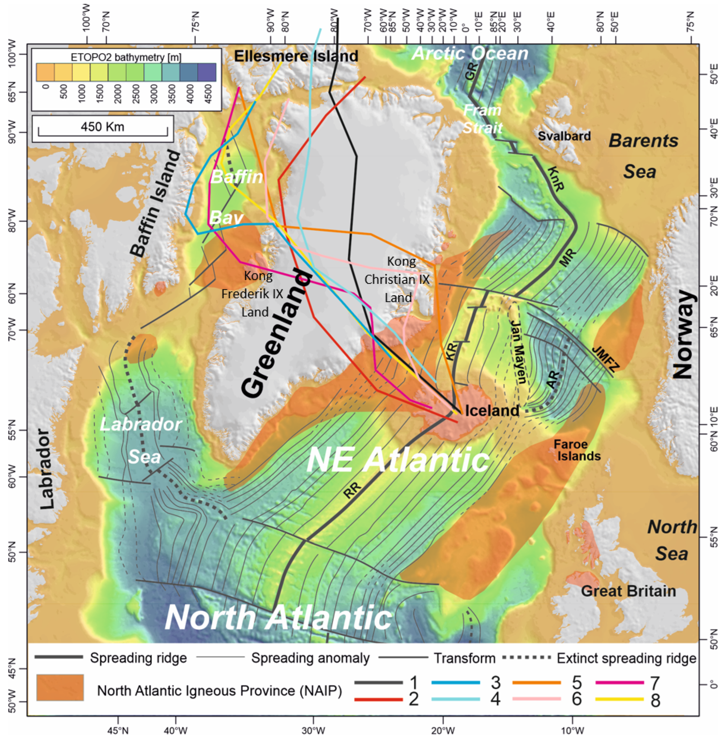
Tectonic and geological overview of the North Atlantic–Labrador Sea/Baffin Bay area (modified from [
6]). Colored lines (numbered 1–8) across Greenland show examples of suggested traces of the Iceland plume since Early Cretaceous: 1: [
12,
18]. 2: [
27]—fixed. 3: [
13]. 4: [
28]. 5: [
29]—moving. 6: [
30]—moving. 7: [
30]—fixed. 8: [
31]. Highlighted polygons: extent of North Atlantic Igneous Province (NAIP). Abbreviations: AR, Aegir Ridge; GR, Gakkel Ridge; JMFZ, Jan Mayen Fracture Zone; KnR, Knipovich Ridge; KR, Kolbeinsey Ridge; MR, Mohns Ridge; RR, Reykjanes Ridge.
Figure 1.
Tectonic and geological overview of the North Atlantic–Labrador Sea/Baffin Bay area (modified from [
6]). Colored lines (numbered 1–8) across Greenland show examples of suggested traces of the Iceland plume since Early Cretaceous: 1: [
12,
18]. 2: [
27]—fixed. 3: [
13]. 4: [
28]. 5: [
29]—moving. 6: [
30]—moving. 7: [
30]—fixed. 8: [
31]. Highlighted polygons: extent of North Atlantic Igneous Province (NAIP). Abbreviations: AR, Aegir Ridge; GR, Gakkel Ridge; JMFZ, Jan Mayen Fracture Zone; KnR, Knipovich Ridge; KR, Kolbeinsey Ridge; MR, Mohns Ridge; RR, Reykjanes Ridge.
2. Method
The nonlinear forward problem is typically generalized as a system of equations , where is a vector of unknown model parameters, contains (known) data, and g() is the nonlinear function which predicts given , to some error .
We seek to infer magnetic crustal thicknesses from the geomagnetic crustal field, as defined by the LCS-1 model of [
32]. Our problem parameterization largely follows [
33]; it is obtained by subdividing the (assumed spherical) Earth’s surface into 25,002 roughly equal-area hexagonal columns (a Goldberg tesselation, via icosahedral subdivision of frequency 50), and using the Equivalent Source Magnetic Dipole method of [
34] to describe the magnetic response of each column, using a dipole placed at the center of each column surface. Our unknown model parameters are thus the individual magnetic crustal thicknesses
and individual magnetic susceptibilities
of each column. The resultant forward problem is expressed by Equation (
1):
where
is a column vector containing magnetic field components at the
N-th query point,
and
are the magnetic susceptibility and magnetic crustal thickness (MCT), respectively, of the crustal column represented by the
N-th dipole, and
is a column vector describing the linear relation between the product
and
. Solutions to Equation (
1) can be approximated through assumptions on the values of
[
33], or by collapsing the parameters into the columnar Vertically Integrated Susceptibility
, but direct inference of
and
for each of the
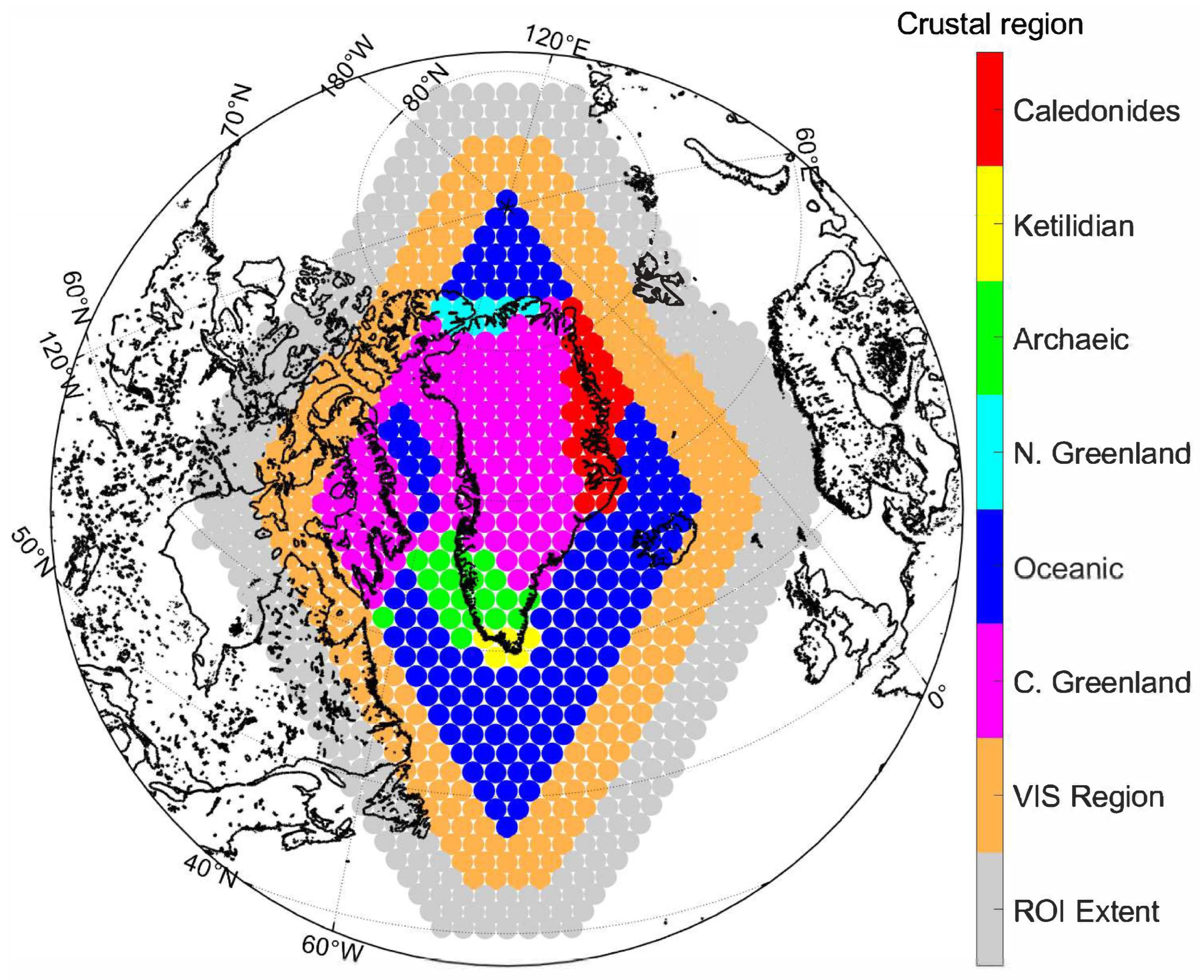
N individual columns is clearly non-unique. Based on known geological correlations and dependencies [
35,
36,
37,
38], we seek to alleviate the non-uniqueness by grouping columns into regions of expected similar crustal composition and, by extension, assumed similar magnetic susceptibilities. Under these assumptions, the forward problem takes the simplified form of Equation (
2):
where the elements of
contains Regional Susceptibilities (RS; identical magnetic susceptibilities for all crustal columns in each of
M crustal regions),
is the vector of individual MCTs, and ∘ denotes the Hadamard product. The assumption of regionally constant magnetic susceptibilities partially alleviates the strong nonlinearity of the problem, but it remains non-unique, leaving Equation (
2) essentially unsolvable for practical purposes in the current formulation.
Fortunately, several pieces of relevant a priori information are available for the components of Equation (
2). We therefore turn to the probabilistic inversion approach [
23,
39], and utilize available a priori information as modeling constraints. Probabilistic inversion essentially treats all input and output information as probability density functions. Assuming an independence between data probability densities and model parameter probability densities, the general probabilistic problem relation is Equation (
3) [
23]:
where
and
are the posterior and prior probability distributions of the model parameters, respectively,
is the likelihood function, and
k is a normalizing constant. We solve Equation (
3) through the extended Metropolis algorithm of [
24], which enables sampling of
if three conditions are met:
- 1.
Samples can be drawn from the prior distribution;
- 2.
The forward problem can be posed in such a way that it is solvable;
- 3.
The likelihood of each solution can be evaluated, i.e., through evaluation of the data residual against a noise model.
A solvable forward problem was defined by Equation (
2), leaving the prior distribution and likelihood evaluation criteria. Regarding the prior distribution, we first seek to reduce the regions in which a priori information is required. This is accomplished by subdividing the inversion into two parts: a nonlinear portion comprises Greenland and its vicinity, where we solve Equation (
3), and a linear portion, which comprises the remainder of the Earth’s crust, solved using the LSQR algorithm of [
40]. Expressing the crustal field in a spherical harmonic expansion, we can view this as a partitioning of contributions to the Gauss coefficients, as shown in Equation (
4):
where
and
are the contributions to the magnetic potential at all query points
from dipoles in the linear and nonlinear regions, respectively. Additional details on the subdivision are provided
Appendix A.
We construct prior probability densities of the magnetic crustal thickness from tomography-inferred Moho depths [
41] and the CRUST1.0 model [
42], while crustal magnetic susceptibility priors are drawn from prior studies, which include the scarce petrophysical measurements available in Greenland and geologically related regions in Finland, Canada and Norway, and oceanic susceptibility estimates [
43,
44,
45,
46,
47,
48,
49,
50,
51,
52,
53,
54,
55,
56,
57,
58,
59,
60,
61]. The compilation of prior information is structured so that the MCT of each crustal column, and the RS for each region, is encoded as individual 1D Gaussian prior probability distributions. An overview of the complete problem parameterization is provided in
Appendix A, while further information on construction of prior distributions and their parameters is provided in
Appendix B.
The data for the inversion are sampled from the satellite data-derived LCS-1 crustal magnetic field model [
32], which we first reduce by subtracting the RVIM0 oceanic remanence model of [
62]. Due to the associated computational requirements, data for all runs are obtained by evaluating the LCS-1 model at 300 km altitude for spherical harmonic degrees
. Coupled with the chosen crustal parameterization, we thereby assume that the ensemble of dipoles, each representing a hexagonal crustal columns approximately ∼160 km wide at the surface, can accurately represent the magnetic crust to within specified uncertainties when viewed from satellite altitude. In order to comply with the input data, modeling results are solely evaluated for the same spherical harmonic range as the data (all contributions to the total model response outside of this range are disregarded). The altitude of evaluation was selected to approximately match the altitude of the original data collection. Given this altitude, evaluation of the LCS-1 model past degree 80 provides progressively lower contributions to the measured magnetic field, due to the rapidly declining power at higher spherical harmonic degrees. On average, the difference between evaluating the LCS-1 model at 300 km altitude up until spherical harmonic degree 80 and spherical harmonic degree 160 is 0.25 nT for the radial component, 0.17 nT for the co-latitudinal component, and 0.17 nT for the longitudinal component.
We assume a purely induced crustal magnetization, with the inducing (core) field taken as spherical harmonic degrees
of the CHAOS-6 model of [
63]. Likelihood evaluation is enabled by associating each datapoint drawn from the LCS-1 model of [
32] with identical standard deviations, i.e., we treat each datapoint as a 1D Gaussian. Since direct evaluation of the data error is not straightforward, several data standard deviation values were tested across multiple different inversions.
Due to the uncertainties concerning crustal thermal parameters required to convert MCT to GTHF, we find complex GTHF modeling unwarranted. Geothermal heat flux estimates from a single-layer 1D (vertical) heat flow model, with a crustal heat production model adopted from [
64], and thermal parameters adopted from [
65], are provided to ease interpretation, but due to the complexity and thus large uncertainty associated with such modeling (e.g., [
66,
67,
68,
69]), the underlying MCT maps are considered the primary result of this study.
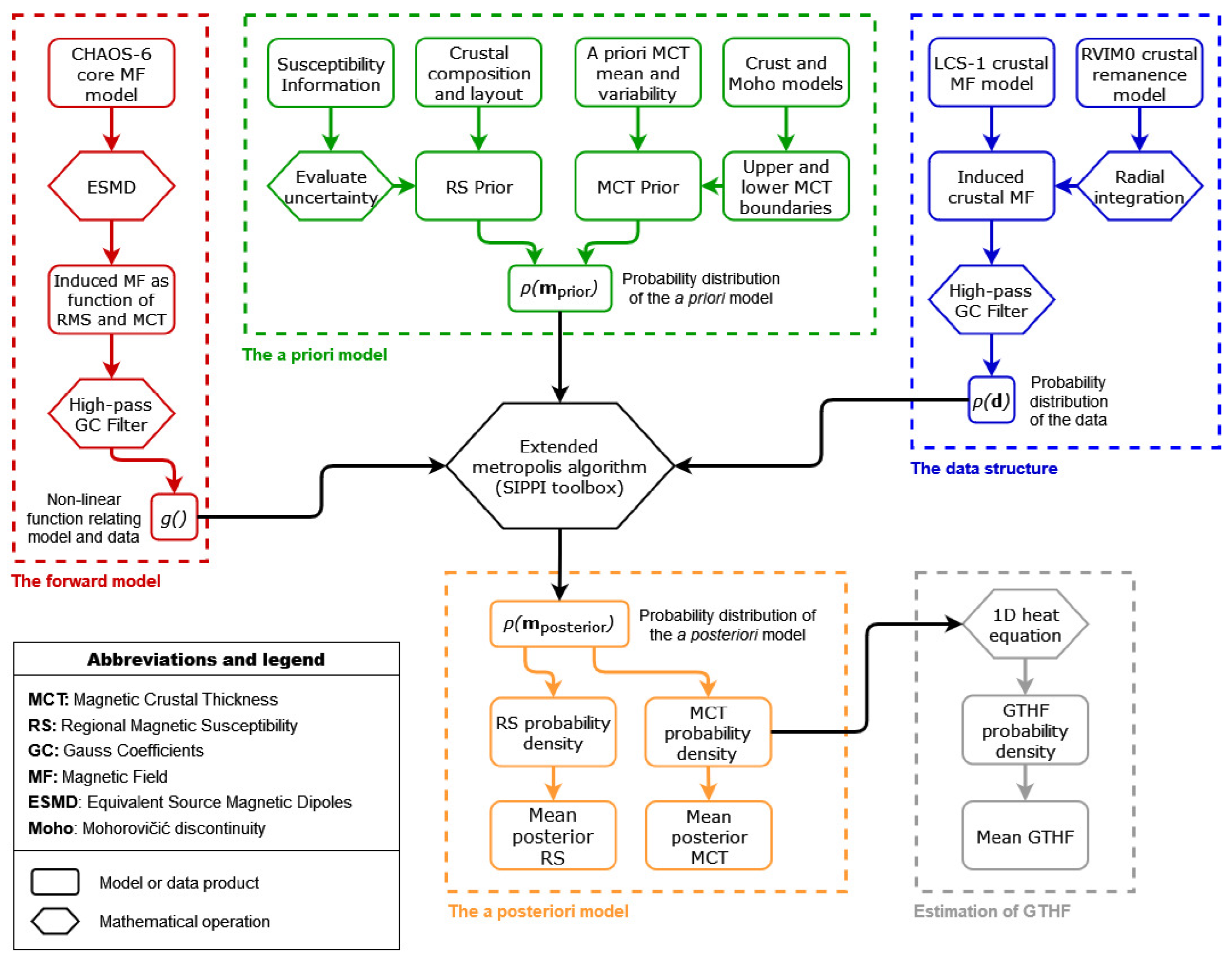
A graphical overview of the data preparation, parameterization, and processing pipeline utilized in the study is provided by
Figure 2. Further details, including the full equations employed in this study, are provided in
Appendix A,
Appendix B,
Appendix C and
Appendix D.
3. Results
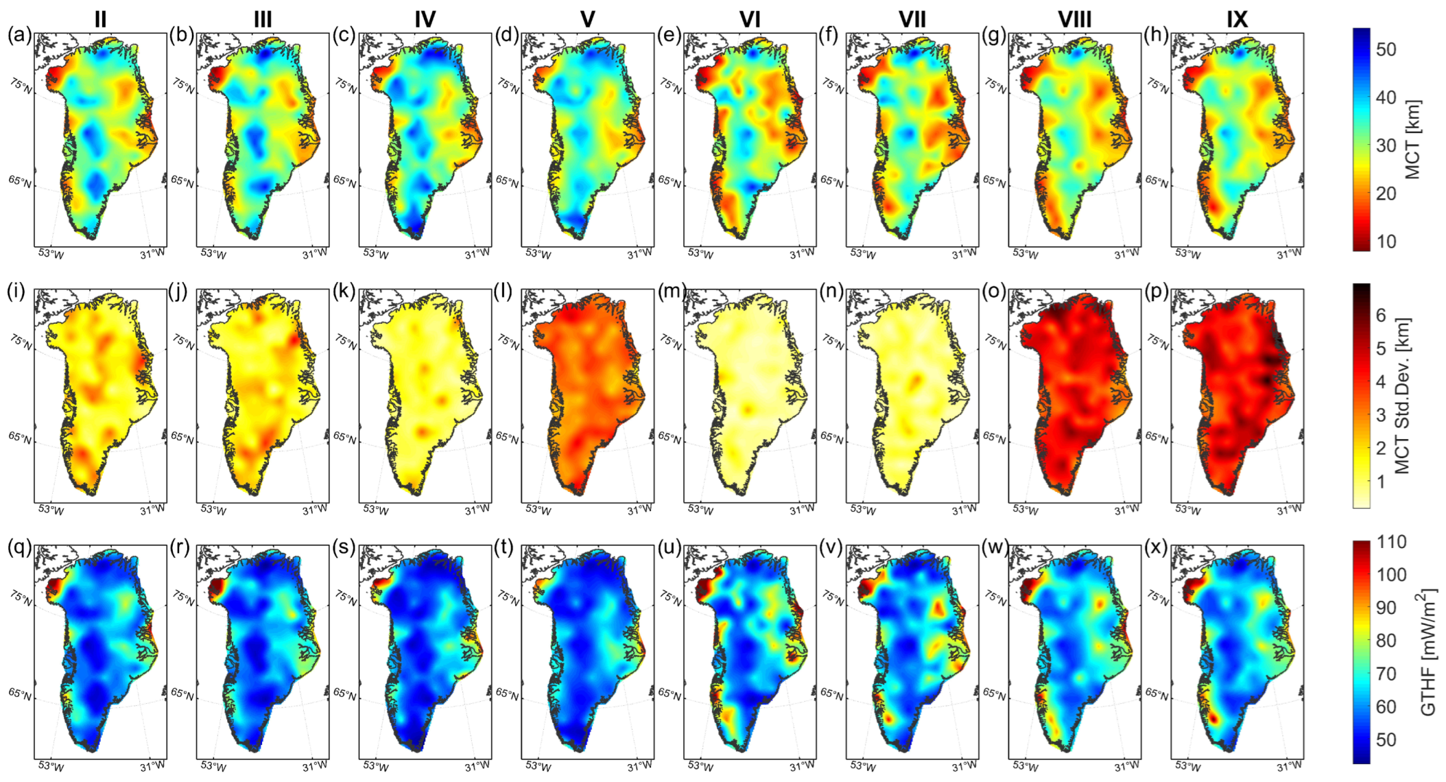
Ten different modeling runs, with differing prior distributions and sampling strategies, were performed. Of these, two were primary runs (denoted Ia and Ib), while the remaining eight (denoted II through IX) were robustness checks with progressively perturbed initial conditions, performed to assess potential impacts of any uncertainties in the governing parameters obtained of the prior and data distributions. Concerns over strong correlations across posterior samples in run Ia led to run Ib being conducted using relaxed conditions, to the point that a few MCT parameters even re-sampled the prior. Run Ib exhibited a high degree of exploration, while retaining overall similarities with run Ia, suggesting that both provide relevant realizations of the posterior model. Overall, we consider run Ib to be the best model based on the amount of posterior samples drawn and its more relaxed conditions.
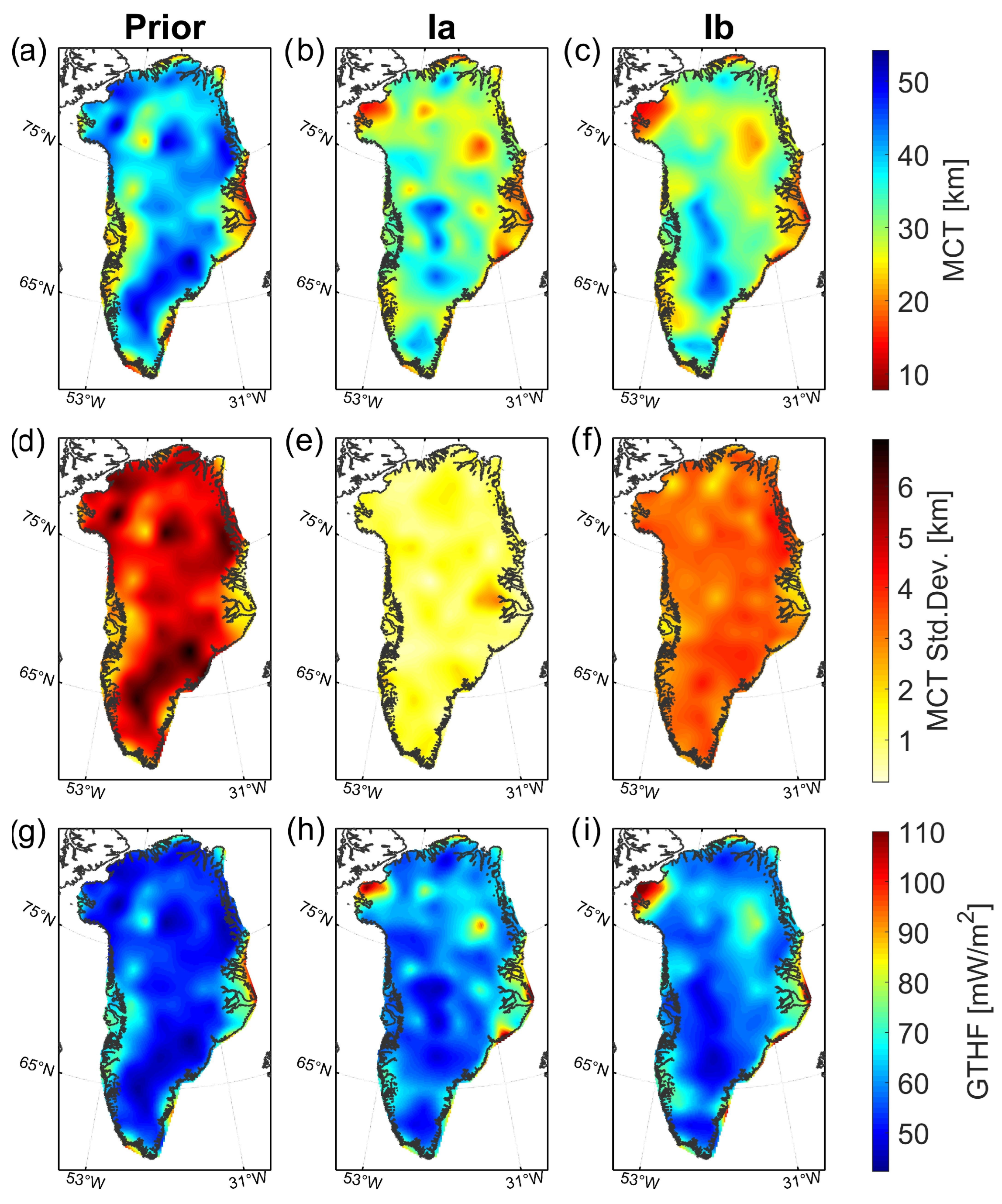
Figure 3 shows the prior MCT and its equivalent GTHF alongside results from the primary runs, while results from the robustness checks are shown in
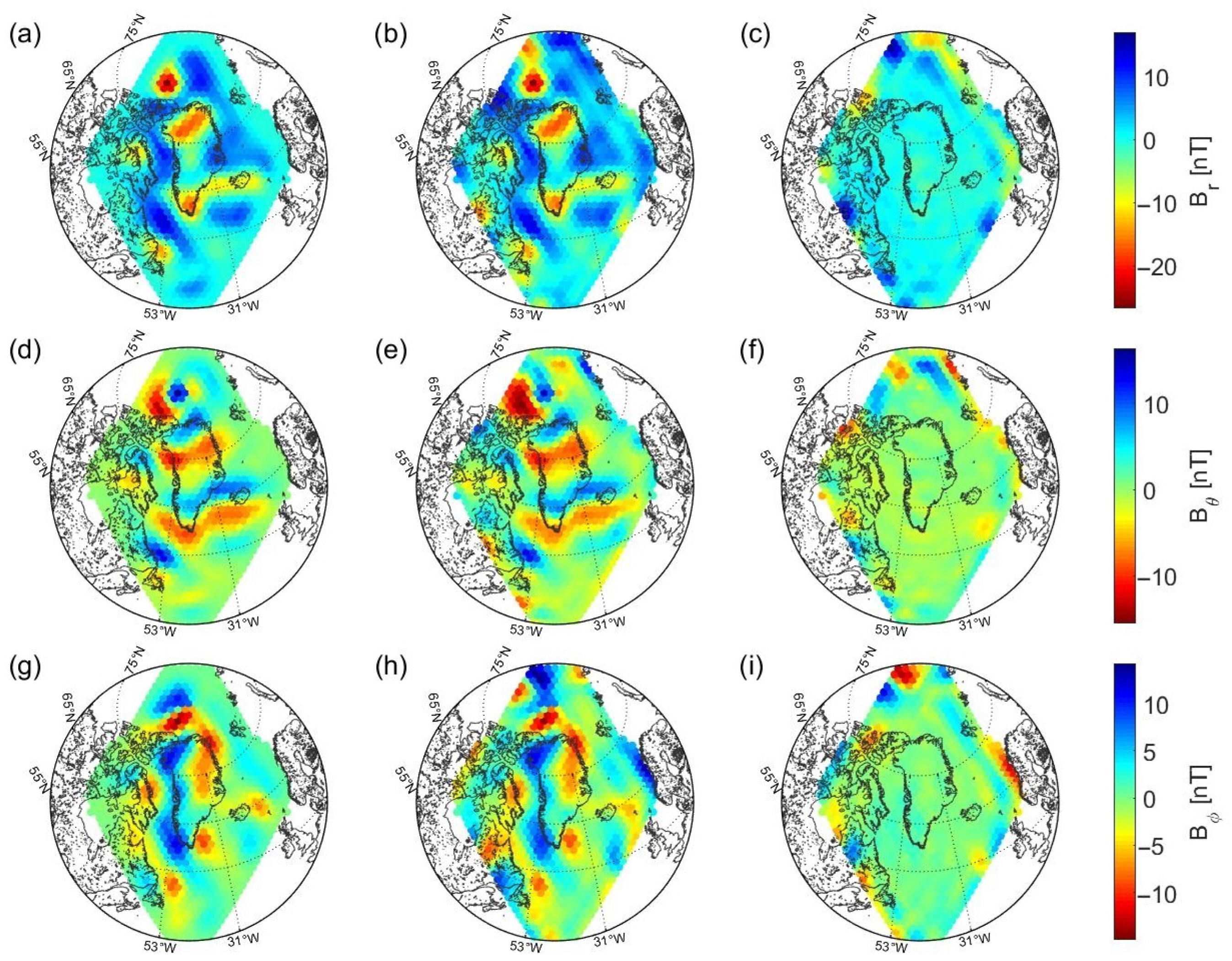
Figure 4. An overview of the data fit of the posterior model from Ib is shown in
Figure 5. Additional information, including the specific parameters for each run, is provided in
Appendix C.
The apparent low MCT standard deviation from run Ia may suggest that an overly constrained sampling has been enforced, given the relatively large amount of model parameters used to fit spherical harmonic degree
data. As such, Run Ia may exhibit some degree of over-fitting, which could also explain the initial suspicions of insufficient model space exploration. Note the difference when using a more exploratory sampling in run Ib, despite using the same initial conditions as run Ia. The similarities between
Figure 3 and
Figure 4, especially the strong correlation of features across their upper and lower rows, reveal a strong robustness in the predicted MCT structures, and by extension, the derived GTHF estimates. Feature robustness is seen across both strictly and loosely constrained models (which exhibit low and high predicted MCT standard deviations, respectively), and regardless of the initial condition perturbations evaluated, suggesting that the nonlinearity of Equation (
1) has been reduced to a point where conclusions may be drawn. Although this does not allow hard conclusions on absolute MCT or GTHF, it provides a general estimate of the former, upon which general conclusions regarding patterns in both MCT and GTHF can be made, given their inverse correlation.
4. Discussion
The nonlinear dependency between MCT and the RS for each region hampers explicit determination of their absolute values, and by extension, absolute GTHF estimation (which is also severely hampered by a lack of knowledge on the thermal properties and layout of the crust). As such, we do not consider it reasonable to estimate the absolute values of MCT, RS, and GTHF based on this study alone. However, relative variations in the robust MCT features provide unique information, and through the inverse correlation between MCT and GTHF, relative traits should be transferable across the two, e.g., as seen across the MCT and GTHF estimates in
Figure 3 and
Figure 4. Except for the structures along the west coast of the southern tip of Greenland, the relative MCT features across all model runs are generally in alignment; we consider this to be our most consequential result.
The parameterization and input data were selected with regard to both computational and investigative feasibility. The latter depends on the assumption that the crustal structures of interest, e.g., mantle plume traces, can be resolved using the magnetic field information utilized, and that corresponding surface features can be captured using ∼160 km wide surface tiles. While the plume stem is believed to be narrow, perhaps 100 km across, and extending down to at least 400–650 km beneath the surface, the plume head may exceed 1000 km in width [
70,
71]. We therefore consider the parameterization to be reasonable for the performed investigation. By fixing the dipole representing each column to the surface, we potentially incur a slight bias in the result. Should this be the case, the bias effect will depend on the MCT; large MCT values in the results may be slight over-estimates, while effects on areas with shallow MCT estimates will be limited. However, considering that the estimated Curie isotherms all relatively shallow when compared to the altitude of the data, we expect that any such potential bias effects will be, at least partially, encompassed by the specified uncertainties.
Note that while there is a clash between essentially-equal-area tessellations and spherical harmonic expansions when nearing the poles (since resolved wavelengths along parallels decrease), any resultant effects only concern variations in one direction, are confined to small wavelengths or areas near the poles, and are expected to be encompassed by the specified data uncertainties to begin with. We therefore expect the influence of such effects to be minor or even negligible, as supported by the high robustness of features towards the poles. The data are thus considered suitable for the parameterization and performed investigations.
Although we argue for the robustness features shown across the MCT maps are indeed real, there are still a few underlying assumptions that could have biased the results. Of these, the subdivision used for susceptibility regions is the hardest constraint, and could carry a significant weight. Especially the large C. Greenland region could prove to have a significant impact on the results. Regardless, the choice was made to proceed with the employed subdivision, primarily for lack of a better alternative.
4.1. No Clear Trace of a Mantle Plume
Given the assumption that a low MCT reflects thinned lithosphere [
72], our model agrees with the general consensus that the Iceland plume withdrew from beneath the Greenland craton in southeastern Greenland, just slightly northeast of the Kangerlussuaq fiord. However, it does not support a straightforward Iceland plume track across the interior of Greenland [
11,
12,
18], such as a simple northwest–southeast or west–east mantle plume trace. Stress testing of the models revealed these findings to be robust across parameter estimates, see
Figure 4.
Comparison with the results of [
17] reveal similarities in the two satellite data-based models. The most prominent similarities are the low MCT in both Kong Christian IX land and Kong Frederik IX land (locations shown in
Figure 1), the ridge of high MCT stretching north–south through north and central western Greenland, the heightened MCT along the southeastern shoreline, and to some extent, the high MCT in northeastern Greenland.
A particularly impactful realization from our results concerns the current modeling meta of plume trace anomalies; given only slight regularization or bias, a significant number of potential plume tracks become viable. Any of these could be favored by a given modeling approach, depending on the employed constraints, regularization and/or alternate biasing, and other underlying assumptions. This suggest a rather clear path forward for more reliable Iceland plume track modeling; assumptions, constraints, or regularization should only be applied with extreme prejudice, due to the ease in which their effects could skew or even dominate the results.
4.2. A Robust Heat Flux Anomaly near NEGIS Origin
All models predict heightened geothermal heat flux beneath the Northeast Greenland Ice Stream (NEGIS), with a significant positive peak immediately beneath its origin. This supports the hypothesis that at least part of NEGIS is driven by an enlarged GTHF. The NEGIS heat flux feature is robust across all modeling runs and consistent with, e.g., [
73], who suggested that the melt anomaly beneath NEGIS may be explained by Iceland plume history. The high melt is further evidenced in radar soundings measurements by [
74], who showed a significant anomaly about 700 km upstream glacier at the origin of NEGIS. In general, heat flux beneath Greenland, and in particular, beneath NEGIS is important to map, as it has huge implications for future behavior of the Greenland Ice Sheet and the ice flow dynamics of NEGIS. Greater geothermal heat flux at the base of an ice mass will impact upon its internal thermal regime and the presence of basal melt water.
The heat flux anomaly beneath east Greenland is, likewise, critical for future behavior of the Greenland Ice Sheet and the earth–ice interaction. Geothermal heat flux at the glacier bedrock is evidence of a warm upper mantle, which affects the response of the solid Earth to the deglaciation process, the glacial isostatic adjustment. A warm upper mantle, as in east Greenland, has a low viscosity, which in turn causes the solid Earth to rebound much faster to deglaciation. Instead of over millennia, the solid Earth can rebound tens of meters within a decade. This Earth feedback mechanism has a stabilizing effect on the evolution of marine-terminating glaciers, and highly influences future estimates of sea level rise. The observed positive heat flux anomaly in east Greenland coincides with a low P-wave velocity perturbation while the confined heat flux anomaly beneath does not appear to be resolved in seismic tomography data [
75].
In the future, a combined effort with ice-sheet modeling may enable explicit determination of GTHF through optimization of only a small number of constants given relative MCT, e.g., as an extension to GTHF model testing, such as those performed by [
21]. We suspect that such a holistic approach may be warranted for, e.g., estimation of general thermal parameters of the crust. In this regard, magnetic data alone may not be sufficient, at least when employed in the form used in this study. The inclusion of additional data types, as well as higher density and better quality magnetic data, may significantly improve MCT and GTHF estimation in the future. Examples of potential sources of data improvement include improved crustal field estimates from satellite magnetic data, and dense high-altitude aeromagnetic data.
Our model is intentionally not constrained using the scarce heat flux measurements available within central Greenland [
20], due to the disproportional spatial representation and weight each datapoint would carry in such a scenario. Should even a single GTHF point-measurement stem from a position or area constituting any kind of heat flux outlier, that datapoint could, in turn, skew the model significantly in an area disproportionally larger than the typical length scale of surface GTHF variation.
5. Conclusions
Our modeling results consistently predict the existence of a heightened heat flux near the onset of the Northeast Greenland Ice Stream. This may be important for subglacial hydrology and modeling ice dynamics of the northeast Greenland outlet glaciers.
Other robustly predicted features include low MCT (and by correlation high GTHF) along an approximately N–S axis in central eastern to central northern Greenland, peaking around the Northeast Greenland Ice Stream, and scattered regions of low heat flux along a similar axis in western Greenland. Other robust features predicted include a number of areas, including on the north and central coast of western Greenland, with low MCT (and high GTHF), which may be related to a potential plume trace. However, we find no clear evidence for an actual plume trace through Greenland; neither a SE–NW or E–W trending trace, nor any other plume trace.
The results highlight the complexity of the solution space, and suggest that even small biases, e.g., due to regularization or simplifying assumptions, could lead to the unintentional favoring of one potential plume track over others during modeling. The multidisciplinary approach demonstrated in this study provides a novel foundation which may, in time, aid in determining a robust, explicit solution to the geothermal heat flux estimation problem.


