
Recognizing the Shape and Size of Tundra Lakes in Synthetic Aperture Radar (SAR) Images Using Deep Learning Segmentation
 , , ,
, , ,  and
and
Abstract
:
1. Introduction
2. Materials and Methods
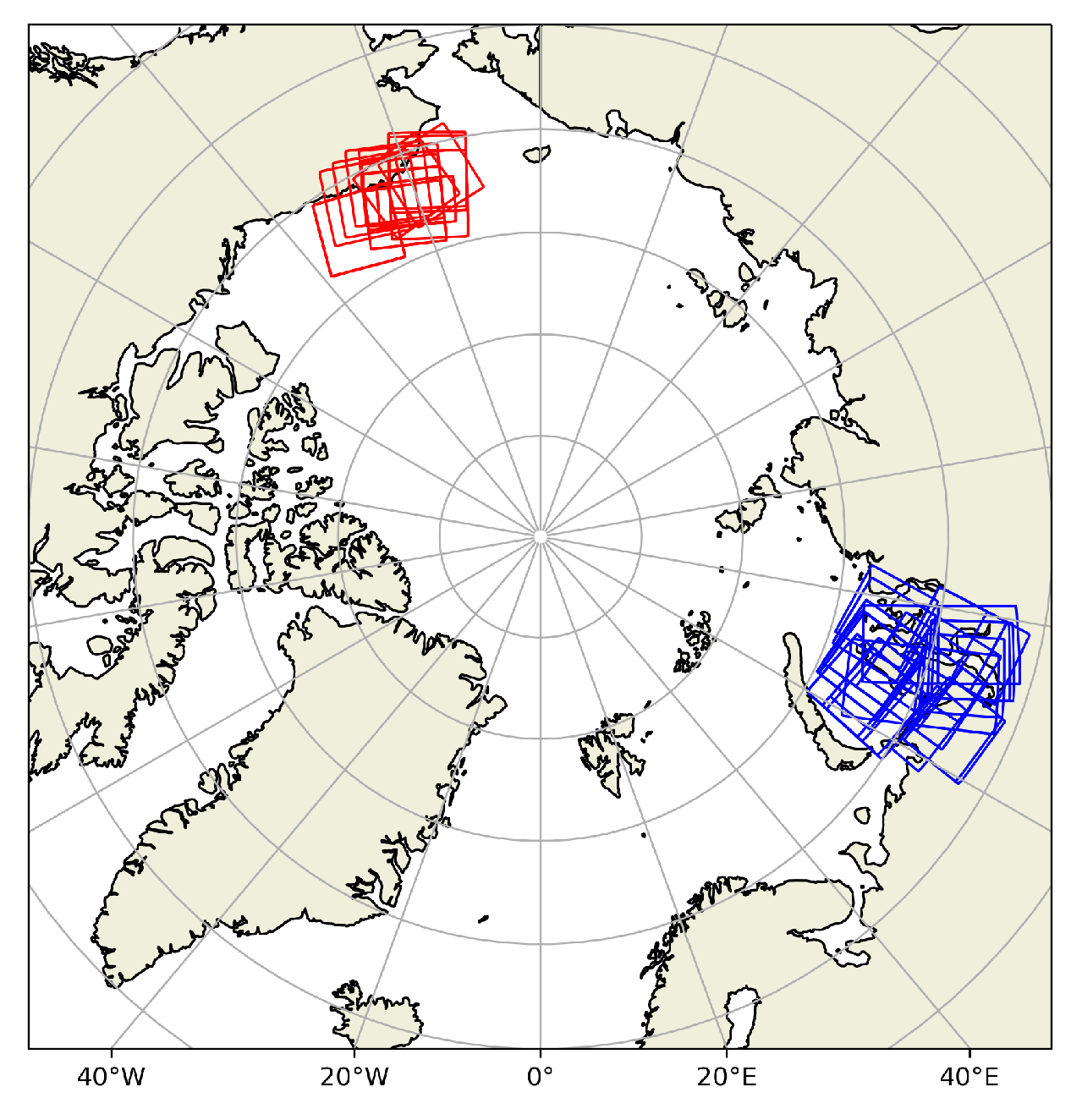
2.1. Satellite SAR Images and Test Sites
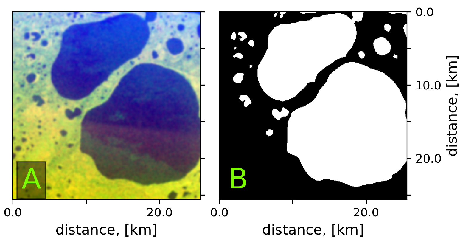
2.2. Manual Mapping of Tundra Lakes
2.3. Automatic Tundra Lake Recognition from SAR Images
| Algorithm 1: Tundra lake shapes recognition from SAR images |
|
2.4. Measuring Trade Features of Segmented Lakes
Box Counting Method
3. Results
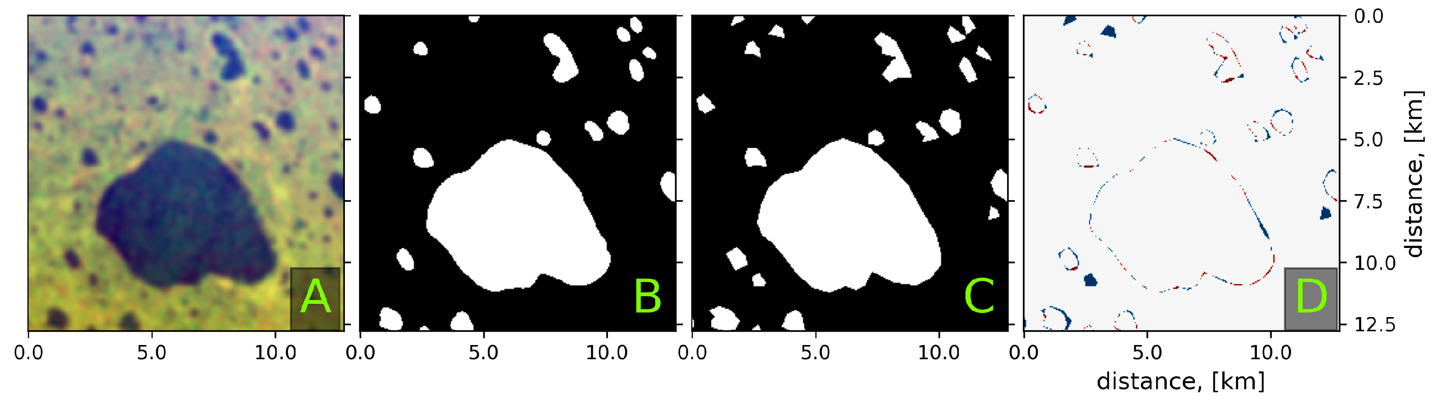
3.1. Tundra Lakes Recognition by U-Net
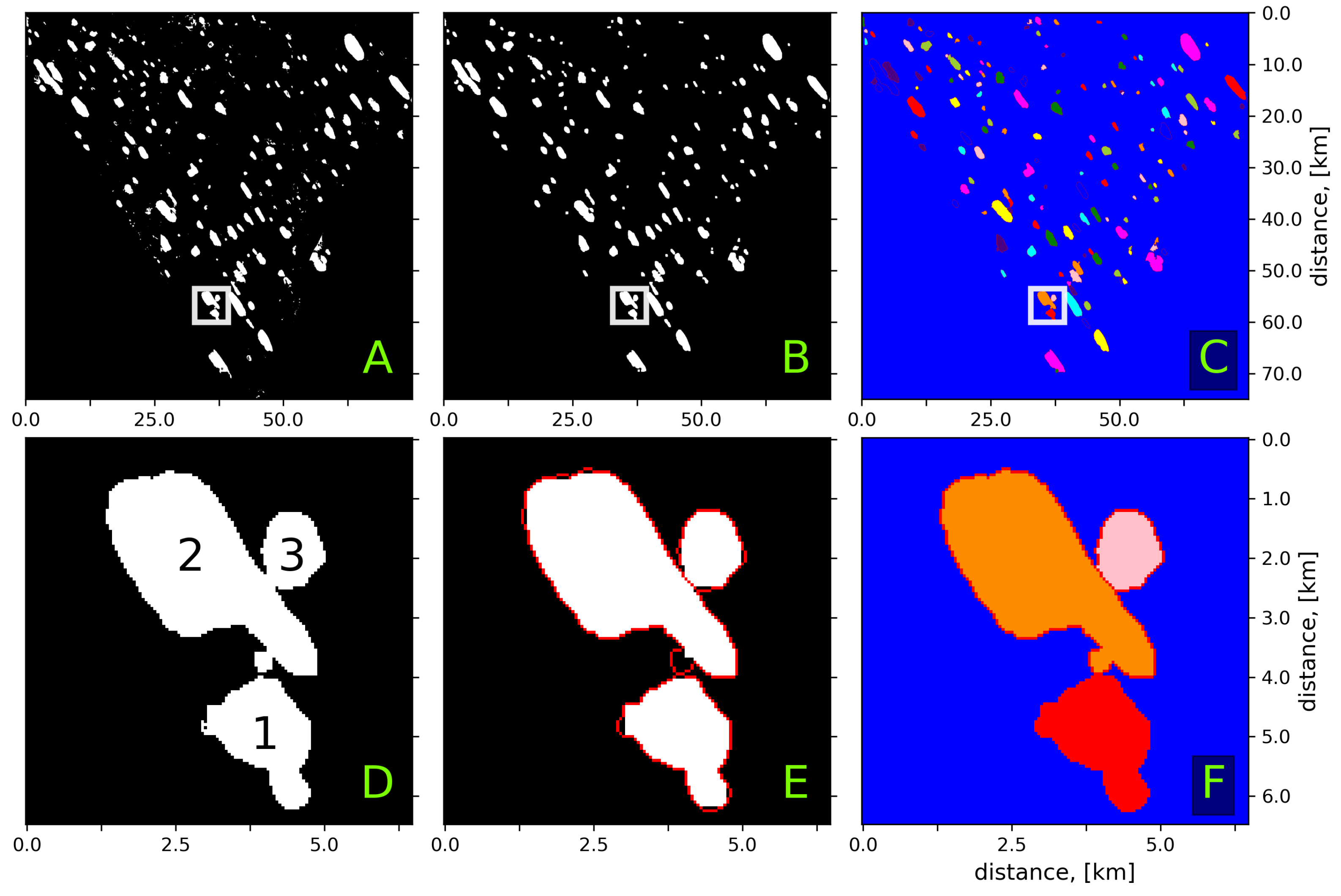
3.2. Instance Segmentation of the Lakes and Noise Filtering
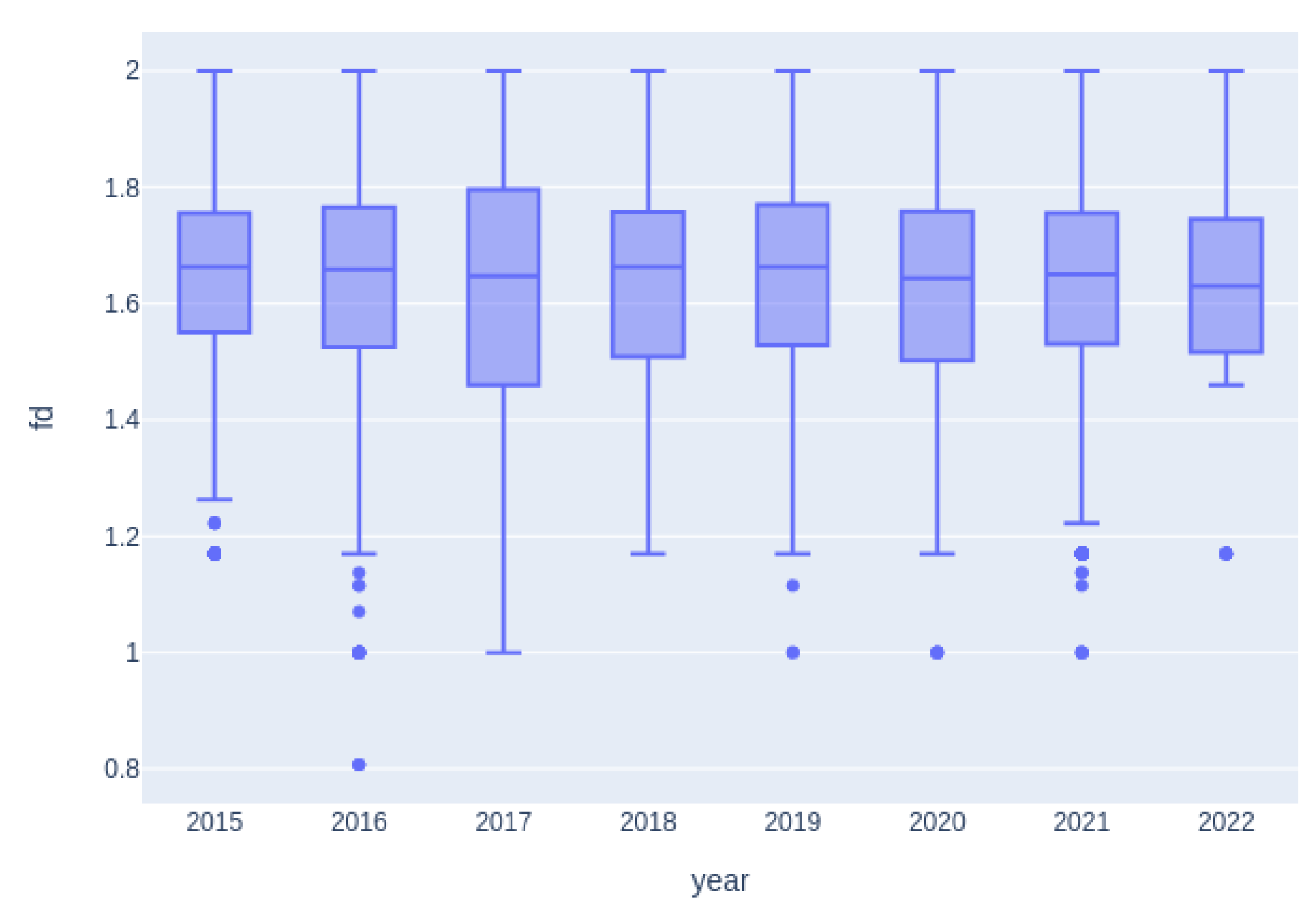
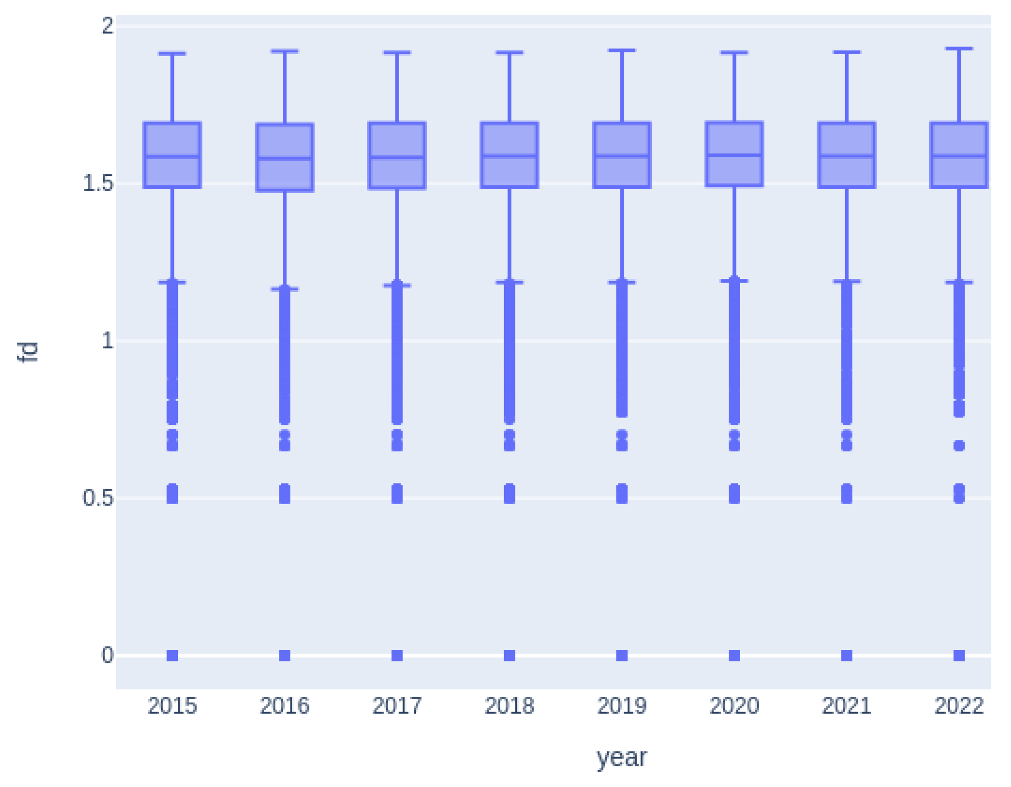
3.3. Fractal Dimension
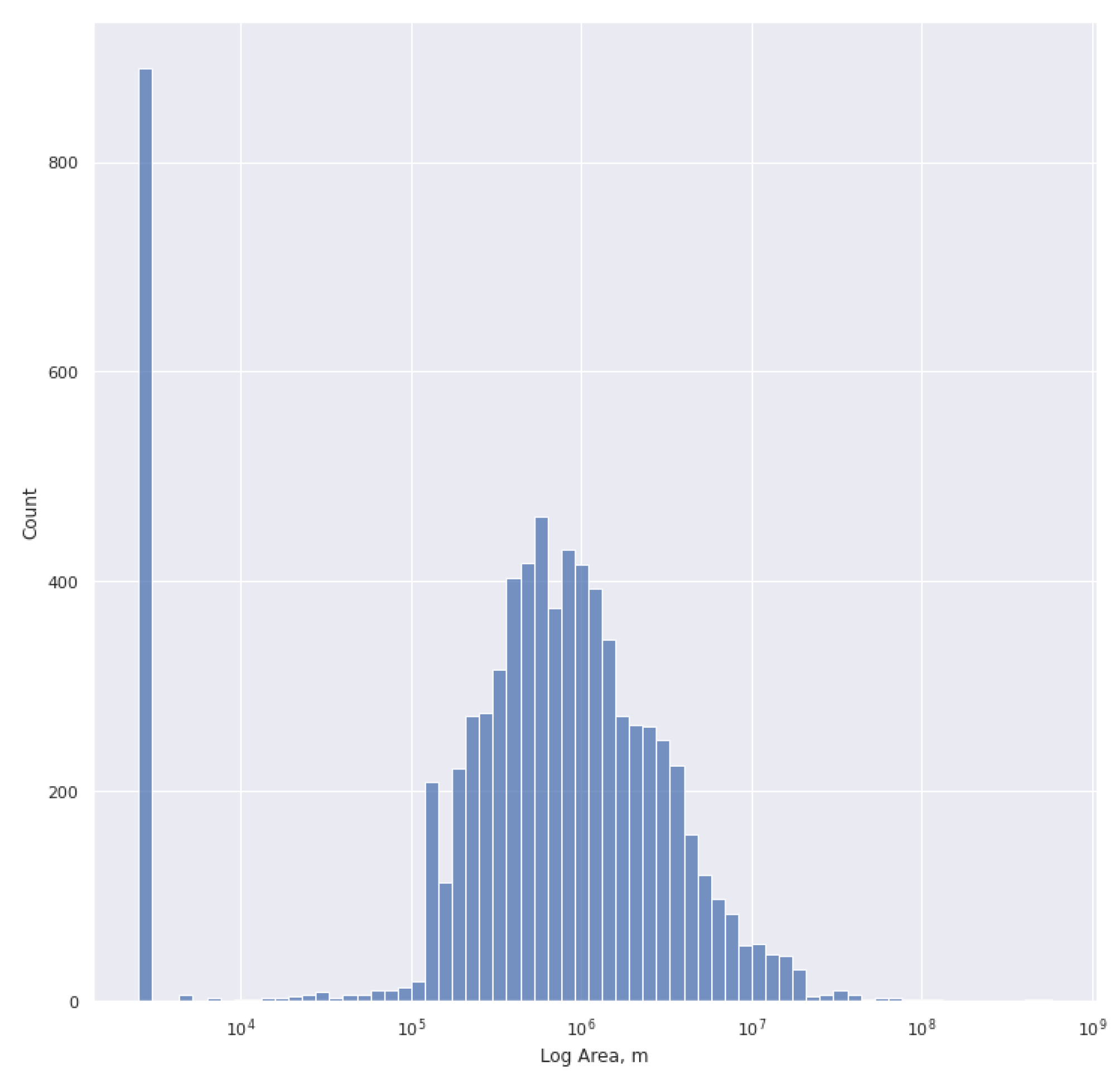
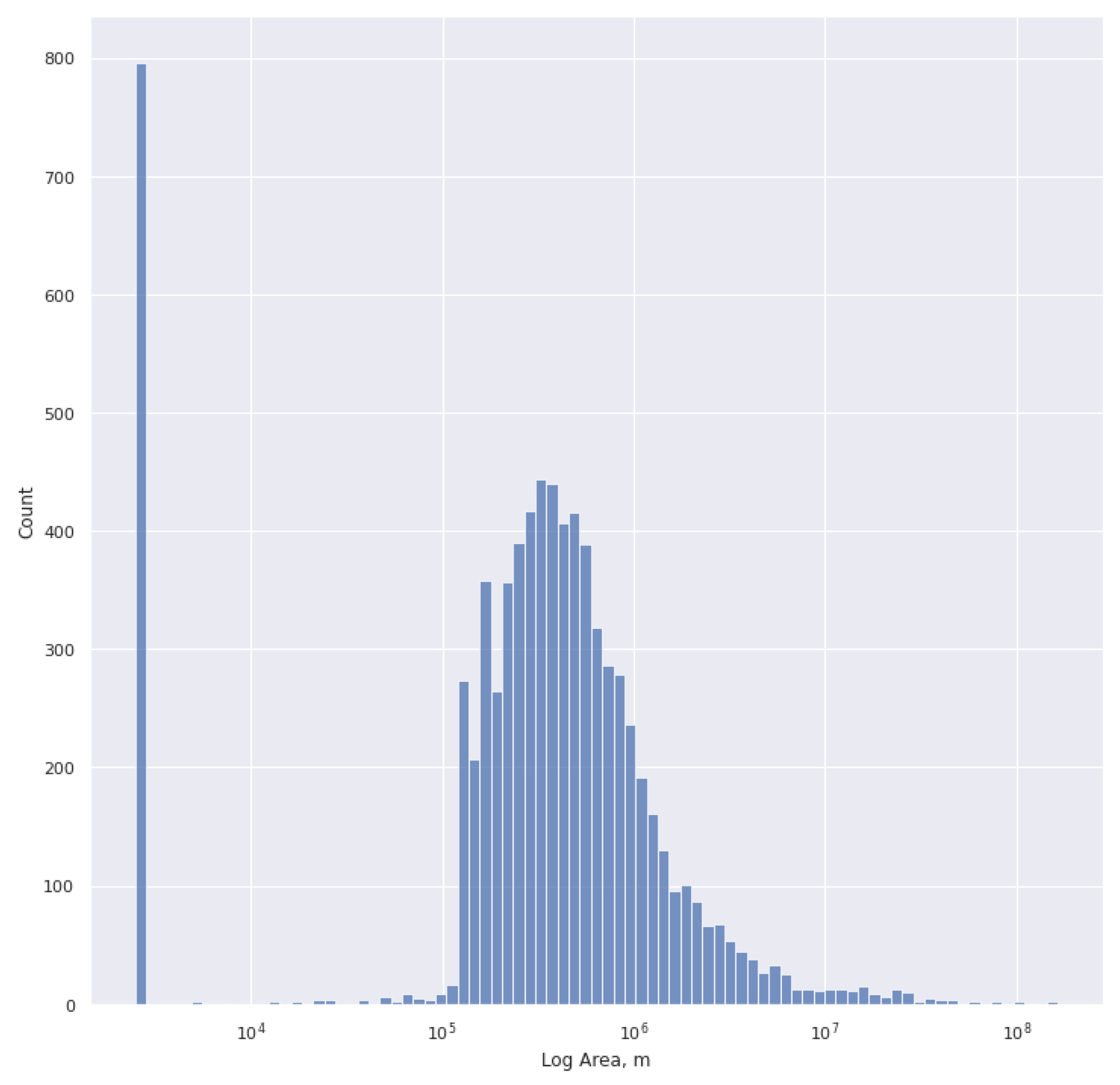
3.4. Size Distribution
4. Discussion
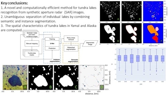
5. Conclusions
Author Contributions
Funding
Data Availability Statement
Acknowledgments
Conflicts of Interest
Abbreviations
| SAR | synthetic aperture radar |
| U-Net | full convolutional neural network architecture |
| InSAR | interferometric synthetic aperture radar |
| IoU (or Jaccard similarity index) | the Intersection of Union metric |
References
- Treat, C.C.; Frolking, S. A permafrost carbon bomb? Nat. Clim. Chang. 2013, 3, 865–867. [Google Scholar] [CrossRef]
- Lawrence, N.S.; O’Sullivan, J.; Parslow, D.; Javaid, M.; Adams, R.C.; Chambers, C.D.; Kos, K.; Verbruggen, F. Training response inhibition to food is associated with weight loss and reduced energy intake. Appetite 2015, 95, 17–28. [Google Scholar] [CrossRef] [PubMed]
- Schädel, C.; Bader, M.K.F.; Schuur, E.A.; Biasi, C.; Bracho, R.; Čapek, P.; De Baets, S.; Diáková, K.; Ernakovich, J.; Estop-Aragones, C.; et al. Potential carbon emissions dominated by carbon dioxide from thawed permafrost soils. Nat. Clim. Chang. 2016, 6, 950–953. [Google Scholar] [CrossRef]
- Kokelj, S.V.; Jorgenson, M. Advances in thermokarst research. Permafr. Periglac. Process. 2013, 24, 108–119. [Google Scholar] [CrossRef]
- Olefeldt, D.; Hovemyr, M.; Kuhn, M.A.; Bastviken, D.; Bohn, T.J.; Connolly, J.; Crill, P.; Euskirchen, E.S.; Finkelstein, S.A.; Genet, H.; et al. The Boreal–Arctic Wetland and Lake Dataset (BAWLD). Earth Syst. Sci. Data 2021, 13, 5127–5149. [Google Scholar] [CrossRef]
- Miner, K.R.; Turetsky, M.R.; Malina, E.; Bartsch, A.; Tamminen, J.; McGuire, A.D.; Fix, A.; Sweeney, C.; Elder, C.D.; Miller, C.E. Permafrost carbon emissions in a changing Arctic. Nat. Rev. Earth Environ. 2022, 3, 55–67. [Google Scholar] [CrossRef]
- Kirpotin, S.; Polishchuk, Y.; Zakharova, E.; Shirokova, L.; Pokrovsky, O.; Kolmakova, M.; Dupre, B. One of the possible mechanisms of thermokarst lakes drainage in West-Siberian North. Int. J. Environ. Stud. 2008, 65, 631–635. [Google Scholar] [CrossRef]
- Jorgenson, J.C.; Jorgenson, M.T.; Boldenow, M.L.; Orndahl, K.M. Landscape change detected over a half century in the Arctic National Wildlife Refuge using high-resolution aerial imagery. Remote Sens. 2018, 10, 1305. [Google Scholar] [CrossRef]
- Shiklomanov, N.I.; Streletskiy, D.A.; Little, J.D.; Nelson, F.E. Isotropic thaw subsidence in undisturbed permafrost landscapes. Geophys. Res. Lett. 2013, 40, 6356–6361. [Google Scholar] [CrossRef]
- Andresen, C.G.; Lougheed, V.L. Disappearing Arctic tundra ponds: Fine-scale analysis of surface hydrology in drained thaw lake basins over a 65 year period (1948–2013). J. Geophys. Res. Biogeosci. 2015, 120, 466–479. [Google Scholar] [CrossRef]
- Karlsson, J.M.; Jaramillo, F.; Destouni, G. Hydro-climatic and lake change patterns in Arctic permafrost and non-permafrost areas. J. Hydrol. 2015, 529, 134–145. [Google Scholar] [CrossRef]
- Boike, J.; Grau, T.; Heim, B.; Günther, F.; Langer, M.; Muster, S.; Gouttevin, I.; Lange, S. Satellite-derived changes in the permafrost landscape of central Yakutia, 2000–2011: Wetting, drying, and fires. Glob. Planet. Change 2016, 139, 116–127. [Google Scholar] [CrossRef]
- Muster, S.; Roth, K.; Langer, M.; Lange, S.; Cresto Aleina, F.; Bartsch, A.; Morgenstern, A.; Grosse, G.; Jones, B.; Sannel, A.B.K.; et al. PeRL: A circum-Arctic permafrost region pond and lake database. Earth Syst. Sci. Data 2017, 9, 317–348. [Google Scholar] [CrossRef]
- Anthony, K.; Zimov, S.; Grosse, G.; Jones, M.C.; Anthony, P.; FS III, C.; Finlay, J.; Mack, M.; Davydov, S.; Frenzel, P.; et al. A shift of thermokarst lakes from carbon sources to sinks during the Holocene epoch. Nature 2014, 511, 452–456. [Google Scholar] [CrossRef] [PubMed]
- Schuur, E.A.; McGuire, A.D.; Schädel, C.; Grosse, G.; Harden, J.W.; Hayes, D.J.; Hugelius, G.; Koven, C.D.; Kuhry, P.; Lawrence, D.M.; et al. Climate change and the permafrost carbon feedback. Nature 2015, 520, 171–179. [Google Scholar] [CrossRef]
- Abbott, B.W.; Jones, J.B.; Schuur, E.A.; Chapin III, F.S.; Bowden, W.B.; Bret-Harte, M.S.; Epstein, H.E.; Flannigan, M.D.; Harms, T.K.; Hollingsworth, T.N.; et al. Biomass offsets little or none of permafrost carbon release from soils, streams, and wildfire: An expert assessment. Environ. Res. Lett. 2016, 11, 034014. [Google Scholar] [CrossRef]
- Nitze, I.; Grosse, G.; Jones, B.M.; Arp, C.D.; Ulrich, M.; Fedorov, A.; Veremeeva, A. Landsat-based trend analysis of lake dynamics across northern permafrost regions. Remote Sens. 2017, 9, 640. [Google Scholar] [CrossRef]
- Muster, S.; Riley, W.J.; Roth, K.; Langer, M.; Cresto Aleina, F.; Koven, C.D.; Lange, S.; Bartsch, A.; Grosse, G.; Wilson, C.J.; et al. Size Distributions of Arctic Waterbodies Reveal Consistent Relations in Their Statistical Moments in Space and Time. Front. Earth Sci. 2019, 7, 2296–6463. [Google Scholar] [CrossRef]
- Carroll, M.L.; Loboda, T.V. Multi-Decadal Surface Water Dynamics in North American Tundra. Remote Sens. 2017, 9, 497. [Google Scholar] [CrossRef]
- Nitze, I.; Grosse, G.; Jones, B.M.; Romanovsky, V.E.; Boike, J. Remote sensing quantifies widespread abundance of permafrost region disturbances across the Arctic and Subarctic. Nat. Commun. 2018, 9, 5423. [Google Scholar] [CrossRef]
- Jawak, S.D.; Kulkarni, K.; Luis, A.J. A review on extraction of lakes from remotely sensed optical satellite data with a special focus on cryospheric lakes. Adv. Remote. Sens. 2015, 4, 196. [Google Scholar] [CrossRef]
- Polishchuk, Y.M.; Bogdanov, A.N.; Polishchuk, V.Y.; Manasypov, R.M.; Shirokova, L.S.; Kirpotin, S.N.; Pokrovsky, O.S. Size distribution, surface coverage, water, carbon, and metal storage of thermokarst lakes in the permafrost zone of the Western Siberia Lowland. Water 2017, 9, 228. [Google Scholar] [CrossRef]
- Karlsson, J.M.; Lyon, S.W.; Destouni, G. Temporal behavior of lake size-distribution in a thawing permafrost landscape in northwestern Siberia. Remote Sens. 2014, 6, 621–636. [Google Scholar] [CrossRef]
- Payne, C.; Panda, S.; Prakash, A. Remote sensing of river erosion on the Colville River, North Slope Alaska. Remote Sens. 2018, 10, 397. [Google Scholar] [CrossRef]
- Naeimi, V.; Bartalis, Z.; Wagner, W. ASCAT soil moisture: An assessment of the data quality and consistency with the ERS scatterometer heritage. J. Hydrometeorol. 2009, 10, 555–563. [Google Scholar] [CrossRef]
- Kerr, Y.; Waldteufel, P.; Wigneron, J.; Martinuzzi, J.; Font, J.M. Berger: Soil moisture retrieval from space: The Soil Moisture and Ocean Salinity (SMOS) mission. IEEE T Geosci. Remote 2001, 39, 1729–1735. [Google Scholar] [CrossRef]
- Jones, B.M.; Grosse, G.; Arp, C.; Jones, M.; Walter Anthony, K.; Romanovsky, V. Modern thermokarst lake dynamics in the continuous permafrost zone, northern Seward Peninsula, Alaska. J. Geophys. Res. Biogeosci. 2011, 116, 0148–0227. [Google Scholar] [CrossRef]
- Schroeder, R.; Rawlins, M.; McDonald, K.; Podest, E.; Zimmermann, R.; Kueppers, M. Satellite microwave remote sensing of North Eurasian inundation dynamics: Development of coarse-resolution products and comparison with high-resolution synthetic aperture radar data. Environ. Res. Lett. 2010, 5, 015003. [Google Scholar] [CrossRef]
- Bartsch, A.; Wagner, W.; Scipal, K.; Pathe, C.; Sabel, D.; Wolski, P. Global monitoring of wetlands–the value of ENVISAT ASAR global mode. J. Environ. Manag. 2009, 90, 2226–2233. [Google Scholar] [CrossRef]
- Sobiech, J.; Dierking, W. Observing lake-and river-ice decay with SAR: Advantages and limitations of the unsupervised k-means classification approach. Ann. Glaciol. 2013, 54, 65–72. [Google Scholar] [CrossRef]
- Widhalm, B.; Bartsch, A.; Heim, B. A novel approach for the characterization of tundra wetland regions with C-band SAR satellite data. Int. J. Remote. Sens. 2015, 36, 5537–5556. [Google Scholar] [CrossRef]
- Hirose, T.; Kapfer, M.; Bennett, J.; Cott, P.; Manson, G.; Solomon, S. Bottomfast Ice Mapping and the Measurement of Ice Thickness on Tundra Lakes Using C-Band Synthetic Aperture Radar Remote Sensing 1. JAWRA J. Am. Water Resour. Assoc. 2008, 44, 285–292. [Google Scholar] [CrossRef]
- Walter, K.M.; Engram, M.; Duguay, C.R.; Jeffries, M.O.; Chapin III, F. The Potential Use of Synthetic Aperture Radar for Estimating Methane Ebullition From Arctic Lakes 1. JAWRA J. Am. Water Resour. Assoc. 2008, 44, 305–315. [Google Scholar] [CrossRef]
- Duguay, C.; Rouse, W.R.; Lafleur, P.M.; Boudreau, L.D.; Crevier, Y.; Pultz, T.J. Analysis of multi-temporal ERS-1 SAR data of subarctic tundra and forest in the northern Hudson Bay Lowland and implications for climate studies. Can. J. Remote. Sens. 1999, 25, 21–33. [Google Scholar] [CrossRef]
- Wakabayashi, H.; Jeffries, M.; Weeks, W. C-band backscatter variation and modelling for lake ice in northern Alaska. J. Remote. Sens. Soc. Jpn. 1994, 14, 220–229. [Google Scholar]
- Liu, L.; Schaefer, K.; Chen, A.; Gusmeroli, A.; Zebker, H.; Zhang, T. Remote sensing measurements of thermokarst subsidence using InSAR. J. Geophys. Res. Earth Surf. 2015, 120, 1935–1948. [Google Scholar] [CrossRef]
- Liu, X.; Guo, Y.; Hu, H.; Sun, C.; Zhao, X.; Wei, C. Dynamics and controls of CO2 and CH4 emissions in the wetland of a montane permafrost region, northeast China. Atmos. Environ. 2015, 122, 454–462. [Google Scholar] [CrossRef]
- Bartsch, A.; Leibman, M.; Strozzi, T.; Khomutov, A.; Widhalm, B.; Babkina, E.; Mullanurov, D.; Ermokhina, K.; Kroisleitner, C.; Bergstedt, H. Seasonal progression of ground displacement identified with satellite radar interferometry and the impact of unusually warm conditions on permafrost at the Yamal Peninsula in 2016. Remote Sens. 2019, 11, 1865. [Google Scholar] [CrossRef]
- Onstott, R.G.; Carsey, F. SAR and scatterometer signatures of sea ice. Microw. Remote. Sens. Sea Ice 1992, 68, 73–104. [Google Scholar]
- Geldsetzer, T.; Sanden, J.v.d.; Brisco, B. Monitoring lake ice during spring melt using RADARSAT-2 SAR. Can. J. Remote. Sens. 2010, 36, S391–S400. [Google Scholar] [CrossRef]
- Jeffries, M.; Morris, K.; Weeks, W.; Wakabayashi, H. Structural and stratigraphie features and ERS 1 synthetic aperture radar backscatter characteristics of ice growing on shallow lakes in NW Alaska, winter 1991–1992. J. Geophys. Res. Ocean. 1994, 99, 22459–22471. [Google Scholar] [CrossRef]
- Merchant, M.A.; Obadia, M.; Brisco, B.; DeVries, B.; Berg, A. Applying Machine Learning and Time-Series Analysis on Sentinel-1A SAR/InSAR for Characterizing Arctic Tundra Hydro-Ecological Conditions. Remote Sens. 2022, 14, 1123. [Google Scholar] [CrossRef]
- Piantanida, R.; Hajduch, G.; Poullaouec, J. Sentinel-1 Level 1 Detailed Algorithm Definition; Techreport SEN-TN-52-7445; ESA: Paris, France, 2016. [Google Scholar]
- Makynen, M.; Manninen, A.T.; Simila, M.; Karvonen, J.A.; Hallikainen, M.T. Incidence angle dependence of the statistical properties of C-band HH-polarization backscattering signatures of the Baltic Sea ice. IEEE Trans. Geosci. Remote. Sens. 2002, 40, 2593–2605. [Google Scholar] [CrossRef]
- Wakabayashi, H.; Weeks, W.; Jeffries, M.O. A C-band backscatter model for lake ice in Alaska. In Proceedings of the IGARSS’93-IEEE International Geoscience and Remote Sensing Symposium, Tokyo, Japan, 18–21 August 1993; pp. 1264–1266. [Google Scholar]
- Zakhvatkina, N.Y.; Alexandrov, V.Y.; Johannessen, O.M.; Sandven, S.; Frolov, I.Y. Classification of sea ice types in ENVISAT synthetic aperture radar images. IEEE Trans. Geosci. Remote. Sens. 2012, 51, 2587–2600. [Google Scholar] [CrossRef]
- Karvonen, J. A sea ice concentration estimation algorithm utilizing radiometer and SAR data. Cryosphere 2014, 8, 1639–1650. [Google Scholar] [CrossRef]
- Karvonen, J. Baltic sea ice concentration estimation using SENTINEL-1 SAR and AMSR2 microwave radiometer data. IEEE Trans. Geosci. Remote. Sens. 2017, 55, 2871–2883. [Google Scholar] [CrossRef]
- Dutta, A.; Gupta, A.; Zissermann, A. VGG Image Annotator (VIA). 2016. Volume 2. Available online: http://www.robots.ox.ac.uk/vgg/software/via (accessed on 10 January 2023).
- Demchev, D.; Sudakow, I. A dataset of 512 × 512 tundra lakes imagery and binary masks from Sentinel-1 in the Yamal and Alaska areas, summer, 2015–2022. Arct. Data Cent. 2023. Available online: https://arcticdata.io/catalog/view/urn%3Auuid%3Aaec6b61a-7318-4680-a39c-85837fa8a5c1 (accessed on 10 January 2023).
- Ronneberger, O.; Fischer, P.; Brox, T. U-net: Convolutional networks for biomedical image segmentation. In Proceedings of the International Conference on Medical Image Computing and Computer-Assisted Intervention, Munich, Germany, 5–9 October 2015; Springer: Berlin/Heidelberg, Germany, 2015; pp. 234–241. [Google Scholar]
- Long, J.; Shelhamer, E.; Darrell, T. Fully convolutional networks for semantic segmentation. In Proceedings of the IEEE Conference on Computer Vision and Pattern Recognition, Boston, MA, USA, 7–12 June 2015; pp. 3431–3440. [Google Scholar]
- Ren, Y.; Li, X.; Yang, X.; Xu, H. Development of a dual-attention U-Net model for sea ice and open water classification on SAR images. IEEE Geosci. Remote. Sens. Lett. 2021, 19, 1–5. [Google Scholar] [CrossRef]
- Sudakow, I.; Asari, V.K.; Liu, R.; Demchev, D. MeltPondNet: A Swin Transformer U-Net for Detection of Melt Ponds on Arctic Sea Ice. IEEE J. Sel. Top. Appl. Earth Obs. Remote. Sens. 2022, 15, 8776–8784. [Google Scholar] [CrossRef]
- Vincent, L.; Soille, P. Watersheds in digital spaces: An efficient algorithm based on immersion simulations. IEEE Trans. Pattern Anal. Mach. Intell. 1991, 13, 583–598. [Google Scholar] [CrossRef]
- Beucher, S.; Meyer, F. The morphological approach to segmentation: The watershed transformation. In Mathematical Morphology in Image Processing; CRC Press: Boca Raton, FL, USA, 2018; pp. 433–481. [Google Scholar]
- Yu, Y.; Acton, S.T. Speckle reducing anisotropic diffusion. IEEE Trans. Image Process. 2002, 11, 1260–1270. [Google Scholar]
- Demchev, D.; Volkov, V.; Kazakov, E.; Alcantarilla, P.F.; Sandven, S.; Khmeleva, V. Sea ice drift tracking from sequential SAR images using accelerated-KAZE features. IEEE Trans. Geosci. Remote. Sens. 2017, 55, 5174–5184. [Google Scholar] [CrossRef]
- Kingma, D.P.; Ba, J. Adam: A method for stochastic optimization. arXiv 2014, arXiv:1412.6980. [Google Scholar]
- Chen, Q.; Yang, X.; Petriu, E.M. Watershed segmentation for binary images with different distance transforms. In Proceedings of the 3rd IEEE International Workshop on Haptic, Audio and Visual Environments and Their Applications, Ottawa, ON, Canada, 2–3 October 2004; Volume 2, pp. 111–116. [Google Scholar]
- Raju, C.N.; Raju, G.; Gottumukkala, V.V. Studies on watershed segmentation for blood cell images using different distance transforms. IOSR J. Vlsi Signal Process. (IOSR-JVSP) 2016, 6, 79–85. [Google Scholar]
- Bradski, G. The OpenCV Library. Dr. Dobb’S J. Softw. Tools 2000, 25, 109–141. [Google Scholar]
- Lovejoy, S. Area-perimeter relation for rain and cloud areas. Science 1982, 216, 185–187. [Google Scholar] [CrossRef]
- Mandelbrot, B. The Fractal Geometry of Nature; W. H. Freeman and Co.: San Francisco, CA, USA, 1982; p. 460. [Google Scholar]
- Klinkenberg, B. A Review of Methods Used to Determine the Fractal Dimension of Linear Features. Math. Geol. 2022, 26, 23–45. [Google Scholar] [CrossRef]
- Oktay, O.; Schlemper, J.; Folgoc, L.L.; Lee, M.; Heinrich, M.; Misawa, K.; Mori, K.; McDonagh, S.; Hammerla, N.Y.; Kainz, B.; et al. Attention u-net: Learning where to look for the pancreas. arXiv 2018, arXiv:1804.03999. [Google Scholar]
- Zhou, Z.; Siddiquee, M.M.R.; Tajbakhsh, N.; Liang, J. Unet++: Redesigning skip connections to exploit multiscale features in image segmentation. IEEE Trans. Med. Imaging 2019, 39, 1856–1867. [Google Scholar] [CrossRef]
- Kugelman, J.; Allman, J.; Read, S.A.; Vincent, S.J.; Tong, J.; Kalloniatis, M.; Chen, F.K.; Collins, M.J.; Alonso-Caneiro, D. A comparison of deep learning U-Net architectures for posterior segment OCT retinal layer segmentation. Sci. Rep. 2022, 12, 14888. [Google Scholar] [CrossRef]
- Seekell, D.A.; Pace, M.L.; Tranvik, L.J.; Verpoorter, C. A fractal-based approach to lake size-distributions. Geophys. Res. Lett. 2013, 40, 517–521. [Google Scholar] [CrossRef]
- Sudakov, I.; Essa, A.; Mander, L.; Gong, M.; Kariyawasam, T. The Geometry of Large Tundra Lakes Observed in Historical Maps and Satellite Images. Remote Sens. 2017, 9, 1072. [Google Scholar] [CrossRef]
- Aleina, F.C.; Brovkin, V.; Muster, S.; Boike, J.; Kutzbach, L.; Sachs, T.; Zuyev, S. A stochastic model for the polygonal tundra based on Poisson–Voronoi diagrams. Earth Syst. Dyn. 2013, 4, 187–198. [Google Scholar] [CrossRef]
- Polishchuk, V.Y.; Polishchuk, Y.M. Geoimitatsionnoe modelirovanie polei termokarstovykh ozer v zonakh merzloty [Geo-Simulation Modeling of Thermokarst Lakes Fields in Permafrost Zones]. Khanty-Mansijsk Uip Yugu 2013, 174, 195–199. [Google Scholar]
- Lopes, R.; Betrouni, N. Fractal and multifractal analysis: A review. Med. Image Anal. 2009, 13, 634–649. [Google Scholar] [CrossRef] [PubMed]
- Nayak, S.R. Analysis of medical images using fractal geometry. In The Research Anthology on Improving Medical Imaging Techniques for Analysis and Intervention; Medical Information Science Reference; IGI Global: Hershey, PA, USA, 2023; pp. 1547–1562. [Google Scholar]
- Sudakow, I.; Pokojovy, M.; Lyakhov, D. Statistical mechanics in climate emulation: Challenges and perspectives. Environ. Data Sci. 2022, 1, e16. [Google Scholar] [CrossRef]


Disclaimer/Publisher’s Note: The statements, opinions and data contained in all publications are solely those of the individual author(s) and contributor(s) and not of MDPI and/or the editor(s). MDPI and/or the editor(s) disclaim responsibility for any injury to people or property resulting from any ideas, methods, instructions or products referred to in the content. |
© 2023 by the authors. Licensee MDPI, Basel, Switzerland. This article is an open access article distributed under the terms and conditions of the Creative Commons Attribution (CC BY) license (https://creativecommons.org/licenses/by/4.0/).
Share and Cite
Demchev, D.; Sudakow, I.; Khodos, A.; Abramova, I.; Lyakhov, D.; Michels, D. Recognizing the Shape and Size of Tundra Lakes in Synthetic Aperture Radar (SAR) Images Using Deep Learning Segmentation. Remote Sens. 2023, 15, 1298. https://doi.org/10.3390/rs15051298
Demchev D, Sudakow I, Khodos A, Abramova I, Lyakhov D, Michels D. Recognizing the Shape and Size of Tundra Lakes in Synthetic Aperture Radar (SAR) Images Using Deep Learning Segmentation. Remote Sensing. 2023; 15(5):1298. https://doi.org/10.3390/rs15051298
Chicago/Turabian StyleDemchev, Denis, Ivan Sudakow, Alexander Khodos, Irina Abramova, Dmitry Lyakhov, and Dominik Michels. 2023. "Recognizing the Shape and Size of Tundra Lakes in Synthetic Aperture Radar (SAR) Images Using Deep Learning Segmentation" Remote Sensing 15, no. 5: 1298. https://doi.org/10.3390/rs15051298