
Impact of SAR Azimuth Ambiguities on Doppler Velocity Estimation Performance: Modeling and Analysis
by
 , , ,
, , ,
Kai Sun
1,2,
Lijie Diao
1,2,
Yawei Zhao
1,
Wenjia Zhao
1,2,
Yongsheng Xu
1,2 and
Jinsong Chong
1,2,* 1
National Key Laboratory of Microwave Imaging Technology, Aerospace Information Research Institute, Chinese Academy of Sciences, Beijing 100190, China
2
School of Electronic, Electrical and Communication Engineering, University of Chinese Academy of Sciences, Beijing 100049, China
*
Author to whom correspondence should be addressed.
Remote Sens. 2023, 15(5), 1198; https://doi.org/10.3390/rs15051198
Submission received: 5 December 2022
/
Revised: 14 February 2023
/
Accepted: 20 February 2023
/
Published: 22 February 2023
(This article belongs to the Special Issue Radar Signal Processing and Imaging for Ocean Remote Sensing)
Abstract
:Doppler Centroid Analysis (DCA) technique is one of the major techniques that do permit a direct retrieval of ocean surface velocity from synthetic aperture radar (SAR) data. However, azimuth ambiguities in the SAR images severely restrict the capability of DCA technique to obtain accurate ocean surface Doppler velocities. Therefore, it is necessary to investigate how the azimuth ambiguities impact the Doppler velocity estimation performance and to evaluate how significant the impact is. In this paper, a model for ocean surface Doppler velocity estimation affected by azimuth ambiguities is developed resorting to jointly circular Gaussian processes, and its statistic is derived. The impact of azimuth ambiguities on Doppler velocity estimation performance in terms of Doppler centroid estimation bias and the standard deviation of Doppler centroid estimates is analyzed. The theoretical results are validated through simulation and Doppler velocities retrieved from Chinese Gaofen-3 (GF-3) SAR Doppler centroid estimates affected by azimuth ambiguities. This study will help researchers better understand the impact of azimuth ambiguities on Doppler velocity estimation, and will provide a theoretical reference for subsequent research on how to reduce the impact of azimuth ambiguities more effectively.
1. Introduction
Measurements of ocean surface velocity are essential to estimate the global transport of salt and heat which regulates our world’s climate, and to reveal surface signatures related to the dynamics of the upper ocean at mesoscale and sub-mesoscale [1,2]. Synthetic aperture radar (SAR), an active microwave imaging sensor, has been a promising means of ocean surface velocity measurement as it dynamically observes the ocean over wide areas under challenging weather conditions, during day or night.
The idea of estimating ocean surface velocity from SAR data using the Doppler centroid analysis (DCA) technique was formulated in 1979 [3] and was first systematically introduced in 2005 [1,4]. Due to simple system requirements and flexible operation, the DCA technique has been further applied and demonstrated in several experiments such as ocean surface currents retrieval [5,6,7,8,9], joint retrieval of ocean surface wind and current [10], strong ocean currents detection [11], and ocean surface feature analysis, etc. [12,13]. The DCA technique essentially estimates the velocities of the scattering elements at the ocean surface along the radial motion of the radar, i.e., the Doppler velocities, through the Doppler shift caused by the relative motion of the target and SAR. The estimated ocean surface velocity is, therefore, highly susceptible to azimuth ambiguities.
Azimuth ambiguities arise in SAR images from finite sampling of the Doppler spectrum at the pulse repetition frequency (PRF). Doppler frequencies higher than the PRF are folded into the central part of the azimuth spectrum so that aliased signals are produced [14,15,16]. The DCA technique works best for images with quasi-uniform normalized radar cross section (NRCS) at moderate to higher winds [17]. The azimuth ambiguities resulting from human-made metallic structures over the ocean and over land near the coast such as ships, oil platforms, big tanks, etc., disrupt the uniformity of the ocean surface NRCS [18,19]. A gradient in NRCS along the azimuth direction within the estimation area will bias Doppler centroid to the brighter part of the illuminated surface [1,20], which results in degradation of ocean surface Doppler velocity estimation performance. Because of the significantly increased NRSC gradient at the land-ocean boundaries, the Doppler velocity estimates in coastal ocean areas are often seriously affected by “ghost targets” of the land due to azimuth ambiguities, making the coastal ocean area one of the biggest focus areas for research. In addition to NRCS modulation, the direct modulation of SAR phase by azimuth ambiguities also leads to a loss of estimation performance [21].
An accurate ocean surface Doppler velocity estimate must take azimuth ambiguities into account. At present, most of research on the impact of azimuth ambiguities on ocean surface Doppler velocity estimation performance still remain at the level of qualitative analysis, and advancements are required.
The purpose of this paper is to develop a model for ocean surface Doppler velocity estimation affected by azimuth ambiguities and to quantitatively analyze the effect of azimuth ambiguities on Doppler velocity estimation based on this model. The model is the basis of analysis, and the quantitative analysis is carried out based on the estimated bias and standard deviation derived from the developed model. The main contributions of our work are summarized as follows:
- (1)
- A model for ocean surface Doppler velocity estimation affected by azimuth ambiguities is developed to investigate how the azimuth ambiguities impact the ocean surface Doppler velocity estimation performance.
- (2)
- Based on the developed model, the estimated bias and standard deviation are derived, and how significant the azimuth ambiguities affect the Doppler velocity estimation performance is quantitatively analyzed.
The remainder of this paper is organized as follows: a model for ocean surface Doppler velocity estimation affected by azimuth ambiguities is developed in Section 2. In Section 3, the impact of azimuth ambiguities on Doppler velocity estimation performance in terms of Doppler velocity estimation bias and the standard deviation of Doppler velocity estimates is quantitatively analyzed. In Section 4, the validation through simulation and Doppler velocities retrieved from Chinese Gaofen-3 (GF-3) SAR Doppler centroid estimates affected by azimuth ambiguities are presented, and conclusions are drawn in Section 5.
2. Model for Ocean Surface Doppler Velocity Estimation Affected by Azimuth Ambiguities
Always with reference to distributed targets, let us consider a single-look complex (SLC) SAR signal affected by azimuth ambiguities, and let us express as the sum of an ambiguity-free signal , from now on referred to as the main signal, and a signal due to the azimuth ambiguity , from now on referred to as the ambiguity signal [16,22]
where is the azimuth (or slow) time and is the range (or fast) time, the azimuth and range time are assumed independent [23], which in essence reduces to the one-dimension model that depends only on the azimuth time
where the main signal and the ambiguity signal are assumed to be complex, Gaussian, zero-mean, and stationary processes orthogonal to each other [24]; thus, the signal is also a complex, Gaussian stationary process with zero mean. By shifting the spectrum of the main signal by and , respectively, and weighing the shifted signal with the azimuth ambiguity ratio (AASR), a time-domain representation of azimuth ambiguity signal can be obtained by performing a IFT (Inverse Fourier Transform) operation. The power of the main signal and the power of the ambiguity signal can be represented by their zero time auto-correlation functions and , respectively,
where stands for the expectation operator.
AASR, an indicator to quantitatively evaluate the degree of azimuth ambiguity of SAR images, is further defined
Since and are stochastic processes, their auto-correlation functions of two samples separated by are, respectively, given by
where is signal sampling interval, . and are the ratios of the magnitude values of auto-correlation function of the main signal and the ambiguity signal to their zero time auto-correlation function values, respectively, which satisfy , . and are phase of and , respectively.
The correlation function of separated by is given by
The expected values of and are equal to zero, as and are assume to be orthogonal to each other. The complex expected value is then given by
where is the phase difference of the auto-correlation function of the ambiguity signal and the main signal.
Due to the fact that the power spectra of the main signal and the ambiguity signal are both modulated by the antenna pattern, their power spectra have the similar shapes, leading to a similar behavior of their auto-correlation function. Then, we can derive and Equation (9) can be simplified
where the phase of the auto-correlation function is as follows:
The Doppler centroid of signal can be estimated from its phase of auto-correlation function by the following formula [23]:
Similarly, the Doppler centroid of the main signal can be estimated following the formula:
The Doppler centroid estimate, affected by azimuth ambiguities, is related to the ocean surface Doppler velocity [1,8]
where is the electromagnetic wavenumber and is the angle of incidence of the radar beam relative to the normal to the surface. The positive Doppler velocity is directed away from the SAR look direction, and the negative Doppler velocity is directed toward the SAR look direction. Please note that this sign convention is identical to that chosen by [25].
3. Statistic of Doppler Velocity Estimation Affected by Azimuth Ambiguities
In this section, the impact of azimuth ambiguities on ocean surface Doppler velocity estimation performance in terms of Doppler centroid estimation bias and the standard deviation of Doppler centroid estimates is analyzed.
3.1. Doppler Velocity Estimation Bias Affected by Azimuth Ambiguities
Considering Equations (12) and (13), the Doppler centroid estimation bias resulting from the presence of the azimuth ambiguity is then given by
Since most SAR systems are only sampled slightly above the Nyquist rate then goes rapidly to zero when k increases and only is of a sufficiently high signal-to noise ratio, hence will usually be preferred. The Doppler centroid estimation bias is thus rewritten as:
According to the error transfer formula, the ocean surface Doppler velocity estimation bias is given by
Substituting Equation (16) into Equation (17), the ocean surface Doppler velocity estimation bias is further given by
For a given radar configuration (radar wavelength, PRF, and incidence angle), the ocean surface Doppler velocity estimation bias has a linear relationship with the Doppler centroid estimation bias. The azimuth ambiguities impact the Doppler centroid estimation bias by modulating the amplitude and by modulating the phase of SAR data.
Figure 1a shows the Doppler centroid estimation bias, as a function of AASR, and the phase difference of the auto-correlation function of the ambiguity signal and the main signal . The figure implies that the Doppler centroid estimation bias depends on both the AASR and the , and is always symmetric about . Figure 1b depicts the absolute value of the Doppler centroid estimation bias variation for several given AASR. The plot highlights the feature that the absolute value of bias is always equal to zero at , regardless of the AASR, while the maximum of the absolute value of bias is determined for a given AASR.
3.2. Standard Deviation of Doppler Velocity Estimates Affected by Azimuth Ambiguities
The standard deviation of the Doppler centroid estimates is related to its auto-correlation magnitude , which can be expressed as follows [23]:
where a data block of range lines, of complex samples each, is assumed to be used for estimation, and . Substituting Equation (10) into Equation (19), the standard deviation of the Doppler centroid estimates can be expressed as:
According to the error transfer formula, the standard deviation of estimated ocean surface Doppler velocity is given by
Substituting Equation (20) into Equation (21), the standard deviation of estimated ocean surface Doppler velocity is further given by
For a given radar configuration, the standard deviation of estimated ocean surface Doppler velocity has a linear relationship with that of the Doppler centroid estimates. The azimuth ambiguities impact the standard deviation of the Doppler centroid estimates by modulating the amplitude and by modulating the phase of SAR data.
Figure 2a illustrates how the standard deviation of the Doppler centroid estimates varies with the AASR, and the phase difference of the auto-correlation function of the ambiguity signal and the main signal . The figure implies that the standard deviation of the Doppler centroid estimates depends on both the AASR and the , and is always symmetric about , as well as . Figure 2b shows the standard deviation of the Doppler centroid estimate variation for several given AASR. The plot highlights some important features: The standard deviation of the Doppler centroid estimates increases as the absolute value of increases and reaches a maximum (minimum) at () for any given . It monotonously decreases when the varies between and , while the opposite occurs between and . The range of the standard deviation variation with respect to is determined when an absolute value of AASR is given.
4. Validation
In the previous sections, a model for ocean surface Doppler velocity estimation affected by azimuth ambiguities has been developed and its statistical properties have been analyzed. In this section, the theoretical results are validated through the simulation and the Doppler velocities retrieved from Chinese GF-3 SAR Doppler centroid estimates affected by azimuth ambiguities.
4.1. Validation with Simulation
The validation with Monte Carlo simulation is carried out in this subsection. Using the model developed in Section 2, the SAR signals affected by the azimuth ambiguities are generated and the ocean surface Doppler velocities are estimated. The parameters of the SAR system and the signals for simulation are summarized in Table 1. Following the parameters in Table 1, the theoretical results are obtained using the equations in Section 3.
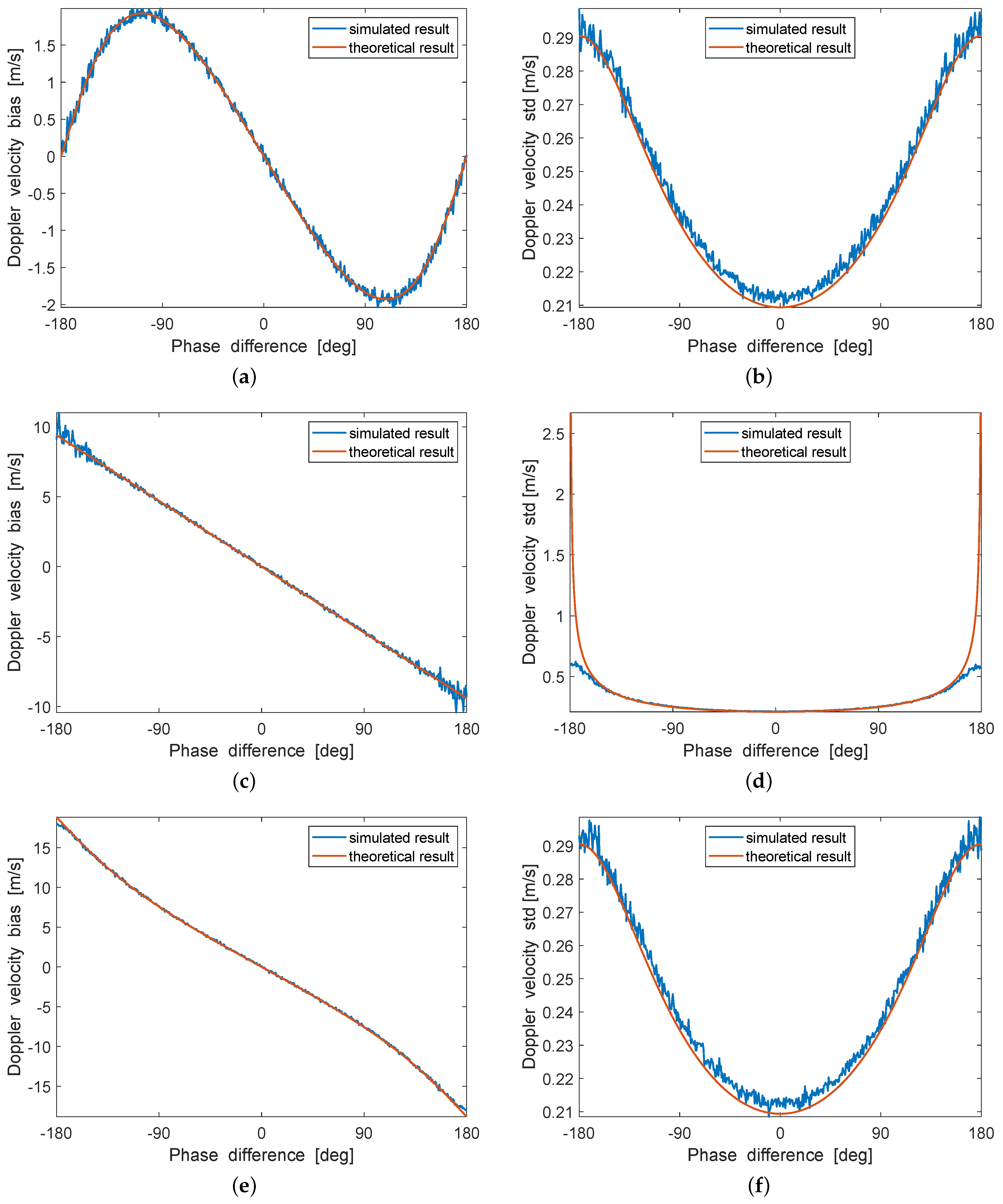
Figure 3 illustrates a comparison of simulated and theoretical results for ocean surface Doppler velocity estimation bias (left panels) and the standard deviation of the ocean surface Doppler velocity estimates (right panels). The results for the comparison with different are displayed, where = −5 dB can be observed in Figure 3a,b, = 0 dB is represented as Figure 3c,d and the ones with = 5 dB is given as Figure 3e,f. The solid blue lines indicate the results obtained by Monte Carlo simulations, on which the solid red lines superimposed indicate the theoretical results. It can be seen that the simulation results and the theoretical results are in good agreement.
The quantitative analysis is performed by using the mean absolute error (MAE), root mean square error (RMSE) and pearson correlation coefficient (PCC), as follows:
where and denote the simulated and theoretical results, respectively, and stand for the average of the simulated and theoretical results, respectively. The quantitative analysis results are shown in Table 2.
4.2. Validation with Chinese GF-3 SAR Data
In this section, validation with Chinese GF-3 SAR data is carried out. GF-3 satellite, launched on 10 August 2016, is China’s first civilian quad-polarized C-band imaging microwave satellite with the highest resolution of 1 m. GF-3 has 12 imaging modes that can provide excellent ocean and coastal monitoring [26,27,28].
Due to the fact that ocean surface velocities vary with different local ocean surface, the Doppler velocity estimation needs to consider both the local AASR and the properties of the local Doppler spectrum. The method for AASR estimation can be found in the literature [16]. As shown in Equation (14), the core of the Doppler velocity estimation is the Doppler centroid estimation. The Doppler centroid estimation methods can be classified into two categories [29], the magnitude-based estimation method in frequency-domain and the phase-based estimation method in time-domain. The frequency-domain estimation methods include the energy balancing estimation method (EBE), correlation with the nominal spectrum estimation method (CNSE) and optimum estimation method (OE). The time-domain estimation method is correlation Doppler centroid estimation method (CDE). Among these methods, the OE has the highest estimation accuracy [24], but it requires accurate azimuth antenna pattern. Due to its high robustness, the CDE method has been widely used since its proposal, and is still used in the latest studies of ocean surface Doppler velocity retrieval [5,30,31,32,33]. Therefore, we use the OE and CDE to validate the proposed model.
Because there is no Doppler centroid estimation method that takes azimuth ambiguity into account, we try the latest method [34] to suppress the azimuth ambiguities in the SAR images at first and then estimate its Doppler centroid. In this way, an ambiguity-free ocean surface Doppler velocity estimates can be obtained. Afterwards, the estimation bias and the standard deviations of estimates are obtained based on the ambiguity-free Doppler velocity estimates and Doppler velocity estimates affected by azimuth ambiguities. Finally, the estimation bias and the standard deviations of estimates are compared with those derived from the model to validate the model.
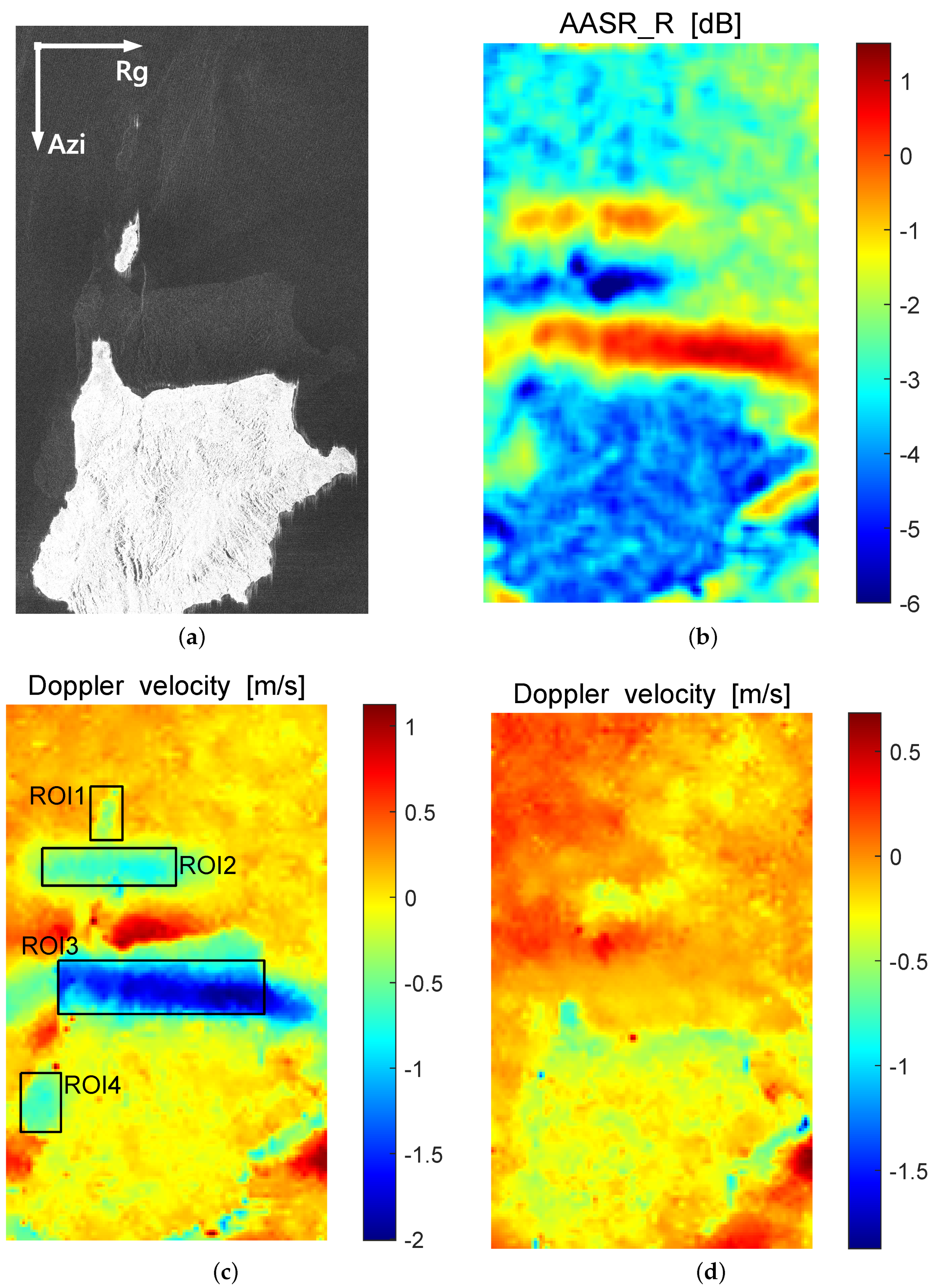
4.2.1. GF-3 SAR Data Affected by the Right Azimuth Ambiguity
Figure 4a shows a GF-3 SAR image with the “ghost target” of the land due to the right azimuth ambiguity. The azimuth (Azi) and range (Rg) directions are indicated by arrows. Figure 4b shows the estimated azimuth ambiguity-to-signal ratio, , due to the right ambiguity. Figure 4c shows the estimated ocean surface Doppler velocity affected by azimuth ambiguities, where the black frame refers to the regions of interest (ROI) that will be used for quantitative analysis below. Figure 4d shows the estimated ocean surface Doppler velocity without azimuth ambiguities.
In the bottom and middle part of Figure 4a, a large and a small island on the ocean can be distinguished. Because of the considerable backscatter difference between the ocean and the islands, ghosts due to azimuth ambiguities are well visible in the image. In Figure 4b, it can be found that the estimated AASR reaches 1 dB within this scene, which indicates that the energy of the azimuth ambiguity signal is greater than that of the ocean surface backscatter. Comparing Figure 4c with Figure 4a, obvious ocean surface Doppler velocity estimation anomalies are observed in the area where the azimuth ambiguities are present. It is worth noting that the distribution characteristics of the ocean surface Doppler velocity anomalies in Figure 4c is consistent with that of the estimated AASR in Figure 4b. Moreover, the larger the value of AASR, the higher the degree of ocean surface Doppler velocity estimation anomalies. These features suggest that the ocean surface Doppler velocity estimation bias induced by the azimuth ambiguities is highly correlated with the AASR. As shown in Figure 4d, the estimated ocean surface Doppler velocity is continuous after azimuth ambiguity suppression, which is consistent with the real ocean surface velocity characteristics. Meanwhile, the island boundaries are clearly visible in the ambiguity-free Doppler velocity map.
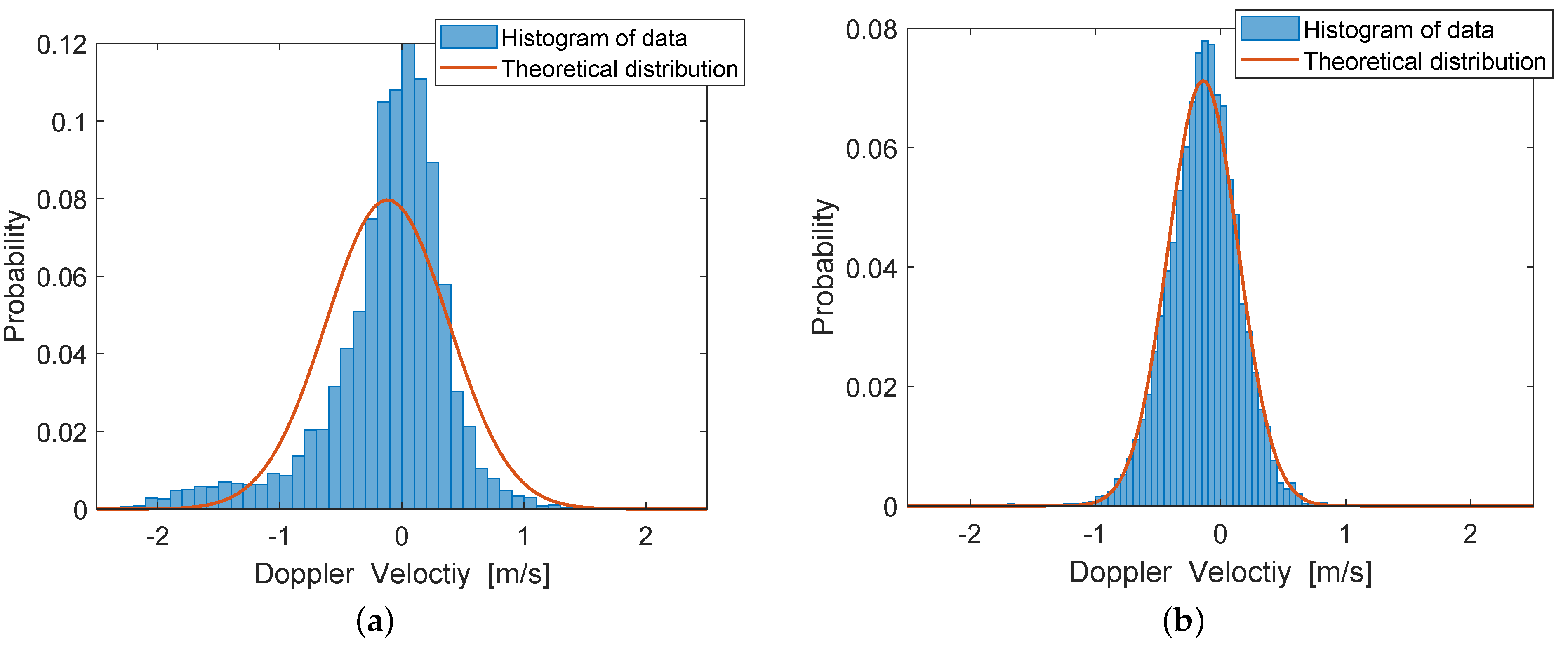
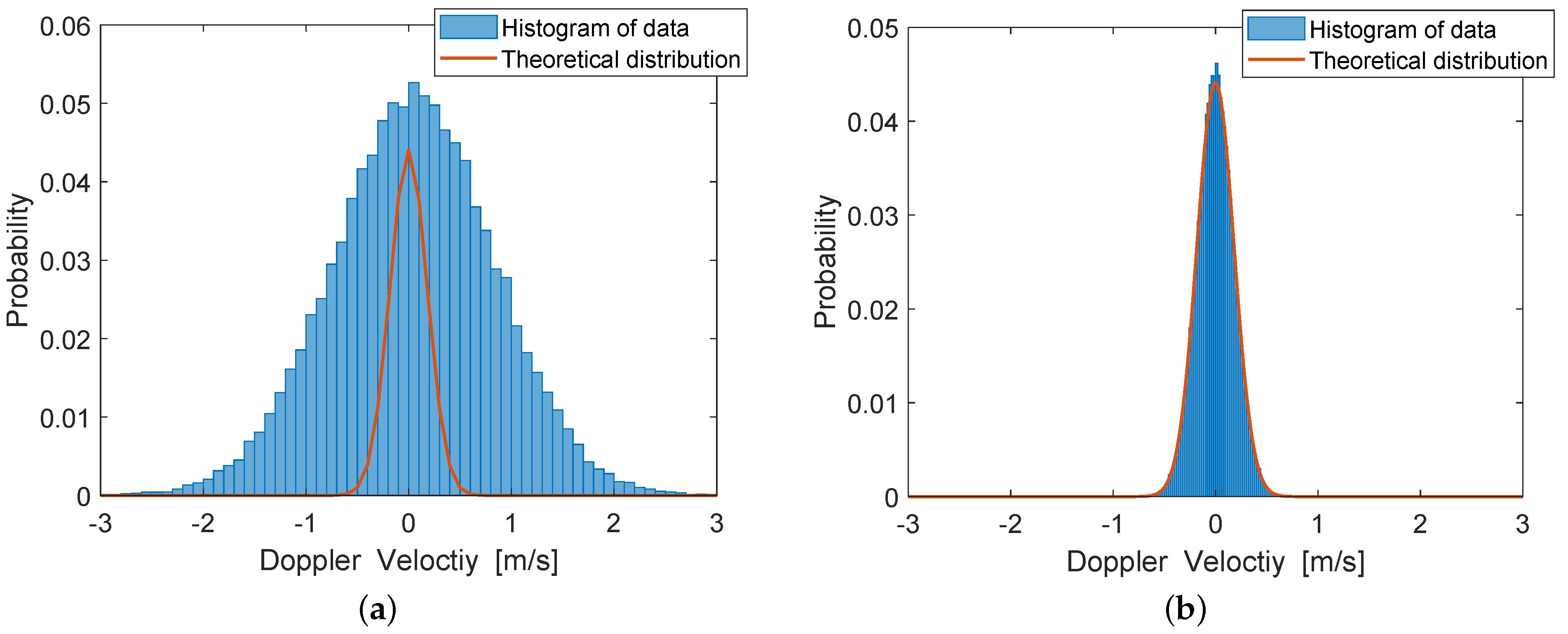
In order to further illustrate the impact of azimuth ambiguities on ocean surface Doppler velocity estimation, statistical analysis of the ocean surface Doppler velocity estimates is carried out. Figure 5a,b exhibit the histograms of the estimated ocean surface Doppler velocity before and after azimuth ambiguity suppression, respectively, where the solid red lines represent the theoretical distribution of ocean surface Doppler velocity without azimuth ambiguities. It can be seen from Figure 5a that the histogram of estimated ocean surface Doppler velocity deviates from the theoretical distribution due to the effect of azimuth ambiguities, while the histogram of ambiguity-free ocean surface Doppler velocity is consistent with the theoretical distribution, as shown in Figure 5b. In addition, the standard deviation of ocean surface Doppler velocity estimates is significantly reduced after azimuth ambiguity suppression. These features suggest that azimuth ambiguities not only degrade the performance of ocean surface Doppler velocity estimation to some extent, but may also modify the distribution of estimated ocean surface Doppler velocity.
Table 3 shows the ocean surface Doppler velocity estimation bias and the standard deviations of ocean surface Doppler velocity estimates within ROI1–ROI4 obtained from GF-3 SAR data, namely measured value, and obtained using the equations in Section 3, namely theoretical value, respectively. The measured values are obtained by the OE and CDE, respectively. It can be seen that the measured values and the theoretical values are in good agreement.
4.2.2. GF-3 SAR Data Affected by the Left and Right Azimuth Ambiguities
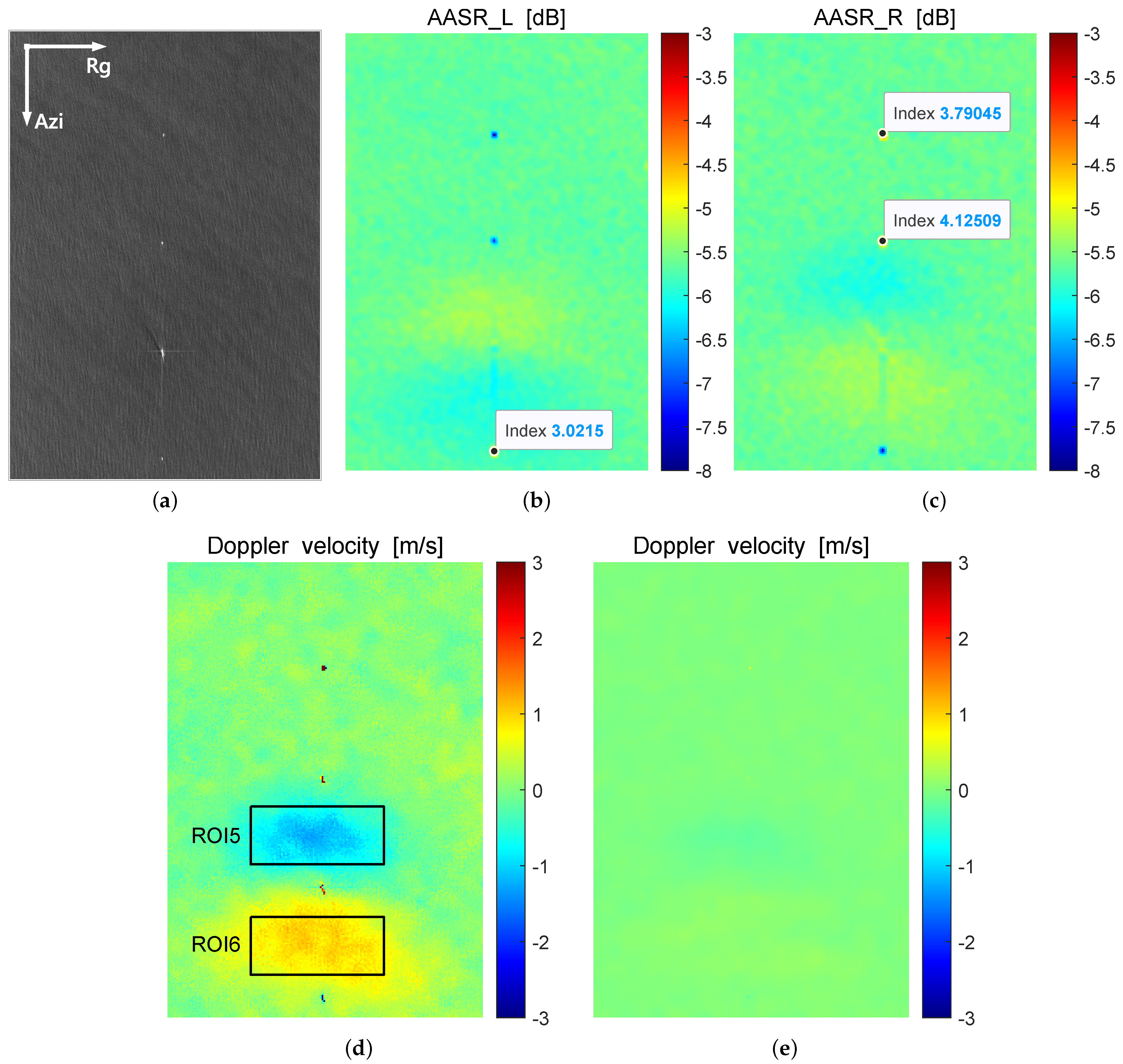
Figure 6a is a GF-3 SAR image affected by ghosts due to left and right azimuth ambiguities. The azimuth (Azi) and range (Rg) directions are indicated by arrows. Figure 6b,c show the estimated azimuth ambiguity-to-signal ratio, and , due to left and right ambiguities, respectively. Figure 6d shows the estimated ocean surface Doppler velocity affected by azimuth ambiguities, in which the black frame areas are the ROIs that will be used for quantitative discussion later. Figure 6e shows the estimated ocean surface Doppler velocity after azimuth ambiguity suppression.
A ship with strong backscatter on the sea and its ghosts due to the first-order and the second-order azimuth ambiguities can be seen in Figure 6a. Comparing Figure 6a with Figure 6b,c, we can find that the two ghosts at the top of the image are due to right azimuth ambiguities, and the ghost at the bottom of the image are due to the left azimuth ambiguity. The estimated AASR in the ghost target regions of ships can reach up to 3 dB as shown in Figure 6b,c. It is worth noting that ocean surface Doppler velocity anomalies appear within ROI5 and ROI6 located between the ship target and its left and right first-order azimuth ambiguities in Figure 6d, while no amplitude anomalies occur at the corresponding locations of the SAR image (see Figure 6a). In addition, the distribution characteristics of the Doppler velocity anomalies in Figure 6d are similar to that of the estimated AASR in Figure 6b,c, which also indicates that the ocean surface Doppler velocity anomalies within ROI5 and ROI6 are due to right and left azimuth ambiguities, respectively. These phenomena imply that the modulation of SAR phase by azimuth ambiguities can lead to a bias in the ocean surface Doppler estimates although the AASR is relatively low in some cases. As shown in Figure 6e, the estimated ocean surface Doppler velocity is continuous after azimuth ambiguity suppression, which is consistent with the real ocean surface velocity characteristics.
In order to further illustrate the impact of azimuth ambiguities on ocean surface Doppler velocity estimation, statistical analysis of the ocean surface Doppler velocity estimates is carried out. Figure 7a,b exhibit the histograms of the estimated ocean surface Doppler velocity before and after azimuth ambiguity suppression, respectively, where the solid red lines represent the theoretical distribution of ocean surface Doppler velocity without azimuth ambiguities. It can be seen from Figure 7a that the histogram of estimated ocean surface Doppler velocity deviates from the theoretical distribution due to the effect of azimuth ambiguities, while the histogram of ambiguity-free ocean surface Doppler velocity is consistent with the theoretical distribution as shown in Figure 7b. In addition, the standard deviation of ocean surface Doppler velocity estimates is significantly reduced after azimuth ambiguity suppression. These features suggest that azimuth ambiguities not only degrade the performance of ocean surface Doppler velocity estimation to some extent, but may also modify the distribution of estimated ocean surface Doppler velocity.
Table 4 shows the ocean surface Doppler velocity estimation bias and the standard deviations of ocean surface Doppler velocity estimates within ROI5 and ROI6 obtained from GF-3 SAR data, namely measured value, and obtained using the equations in Section 3, namely theoretical value, respectively. The measured values are obtained by the OE and CDE, respectively. The measured values and the theoretical values are in good agreement.
5. Conclusions
In this paper, a model for ocean surface Doppler velocity estimation affected by azimuth ambiguities is developed. The impact of azimuth ambiguities on Doppler velocity estimation performance in terms of Doppler centroid estimation bias and the standard deviation of Doppler centroid estimates is analyzed. The theoretical results are validated through simulation and Doppler velocities retrieved from Chinese GF-3 SAR Doppler centroid estimates.
Azimuth ambiguities affect the performance of ocean surface Doppler velocity estimation by modulating the amplitude and the phase of SAR data. The Doppler centroid estimation bias and the standard deviation of the Doppler centroid estimates depend on the AASR as well as the phase difference of the auto-correlation function of the ambiguity signal and the main signal. The range of variations of bias and the standard deviations is only AASR dependent.
Both the results for simulation and experiments on GF-3 SAR data are in good agreement with theoretical results. Validation reveals that azimuth ambiguities not only degrade the performance of ocean surface Doppler velocity estimation, but also may modify the distributions of estimated ocean surface Doppler velocities.
This study can be used not only to pre-check the quality of SAR data and eliminate the data that cannot meet the estimation accuracy requirements from the user community, but also to assess how well the ocean surface Doppler velocity estimated from the available data can serve the application.
Our future work could involve an improved method for estimating ocean surface Doppler velocities from SAR data, in which the uncertainties in Doppler velocity estimates due to azimuth ambiguities would be taken into account as part of the cost function. Ocean surface Doppler velocity contains contributions from ocean surface motion induced by winds, waves and currents. After correction of bias caused by wind–wave-induced contributions, future work would also focus on the detection, estimation and interpretation of mesoscale processes related to ocean surface currents, such as ocean fronts, mesoscale eddies, and internal waves.
Author Contributions
Conceptualization, K.S. and J.C.; methodology, K.S.; validation, K.S., L.D. and W.Z.; formal analysis, K.S., Y.Z. and Y.X.; writing—original draft preparation, K.S.; writing—review and editing, K.S. and J.C.; funding acquisition, J.C. All authors have read and agreed to the published version of the manuscript.
Funding
This research was funded by the National Natural Science Foundation of China (No. 62231024) and the National Key R&D Program of China (No. 2022YFC3104900/2022YFC3104904).
Data Availability Statement
Not applicable.
Conflicts of Interest
The authors declare no conflict of interest.
References
- Chapron, B.; Collard, F.; Ardhuin, F. Direct measurements of ocean surface velocity from space: Interpretation and validation. J. Geophys. Res. 2005, 110, C07008. [Google Scholar] [CrossRef]
- Rouault, M.J.; Mouche, A.; Collard, F.; Johannessen, J.A.; Chapron, B. Mapping the Agulhas Current from space: An assessment of ASAR surface current velocities. J. Geophys. Res. 2010, 115, C10026. [Google Scholar] [CrossRef]
- Shuchman, R.; Rufenach, C.; Gonzalez, F.; Klooster, A. The feasibility of measurement of ocean current detection using SAR data. In Proceedings of the 2013 IEEE International Geoscience and Remote Sensing Symposium, Melbourne, Australia, 21–26 July 2003. [Google Scholar]
- Elyouncha, A.; Eriksson, L.E.B.; Johnsen, H. Direct Comparison of Sea Surface Velocity Estimated From Sentinel-1 and TanDEM-X SAR Data. IEEE J. Sel. Top. Appl. Earth Obs. Remote Sens. 2022, 15, 2425–2436. [Google Scholar] [CrossRef]
- Zamparelli, V.; De Santi, F.; Cucco, A.; Zecchetto, S.; De Carolis, G.; Fornaro, G. Surface currents derived from SAR Doppler processing: An analysis over the naples coastal region in south Italy. J. Mar. Sci. Eng. 2020, 8, 203. [Google Scholar] [CrossRef]
- Moiseev, A.; Johnsen, H.; Hansen, M.; Johannessen, J. Evaluation of Radial Ocean Surface Currents Derived from Sentinel-1 IW Doppler Shift Using Coastal Radar and Lagrangian Surface Drifter Observations. J. Geophys. Res. Ocean. 2020, 125, e2019JC015743. [Google Scholar] [CrossRef]
- Moiseev, A.; Johnsen, H.; Johannessen, J.A.; Collard, F.; Guitton, G. On removal of sea state contribution to sentinel–1 doppler shift for retrieving reliable ocean surface current. J. Geophys. Res. Ocean. 2020, 125, e2020JC016288. [Google Scholar] [CrossRef]
- Hansen, M.W.; Collard, F.; Dagestad, K.F.; Johannessen, J.A.; Fabry, P.; Chapron, B. Retrieval of Sea Surface Range Velocities from Envisat ASAR Doppler Centroid Measurements. IEEE Trans. Geosci. Remote Sens. 2011, 49, 3582–3592. [Google Scholar] [CrossRef]
- Yang, X.; He, Y. Retrieval of a Real-Time Sea Surface Vector Field from SAR Doppler Centroid: 1. Ekman Current Retrieval. J. Geophys. Res. Ocean. 2023, 128, e2022JC018657. [Google Scholar] [CrossRef]
- Elyouncha, A.; Eriksson, L.E.B.; Broström, G.; Axell, L.; Ulander, L.H.M. Joint retrieval of ocean surface wind and current vectors from satellite SAR data using a Bayesian inversion method. Remote Sens. Environ. 2021, 260, 112455. [Google Scholar] [CrossRef]
- Biron, K.; Van Wychen, W.; Vachon, P.W. Gulf stream detection from SAR Doppler anomaly. Can. J. Remote Sens. 2019, 44, 311–320. [Google Scholar] [CrossRef]
- Van Wychen, W.; Vachon, P.W.; Wolfe, J.; Biron, K. The utility of Sentinel-1 data for ocean surface feature analysis in the vicinity of the Gulf Stream. Can. J. Remote Sens. 2018, 44, 144–152. [Google Scholar] [CrossRef]
- Van Wychen, W.; Vachon, P.W.; Wolfe, J.; Biron, K. Synergistic RADARSAT-2 and Sentinel-1 SAR images for ocean feature analysis. Can. J. Remote Sens. 2019, 45, 591–602. [Google Scholar] [CrossRef]
- Moreira, A. Suppressing the azimuth ambiguities in synthetic aperture radar images. IEEE Trans. Geosci. Remote Sens. 1993, 31, 885–895. [Google Scholar] [CrossRef]
- Li, F.k.; Johnson, W.T.K. Ambiguities in Spacebornene Synthetic Aperture Radar Systems. IEEE Trans. Aerosp. Electron. Syst. 1983, 3, 389–397. [Google Scholar] [CrossRef]
- Villano, M.; Krieger, G. Spectral-Based Estimation of the Local Azimuth Ambiguity-to-Signal Ratio in SAR Images. IEEE Trans. Geosci. Remote Sens. 2014, 52, 2304–2313. [Google Scholar] [CrossRef]
- Johannessen, J.A.; Chapron, B.; Collard, F.; Kudryavtsev, V.; Mouche, A.; Akimov, D.; Dagestad, K.F. Direct ocean surface velocity measurements from space: Improved quantitative interpretation of Envisat ASAR observations. Geophys. Res. Lett. 2008, 35, L22608. [Google Scholar] [CrossRef]
- Vespe, M.; Greidanus, H. SAR Image Quality Assessment and Indicators for Vessel and Oil Spill Detection. IEEE Trans. Geosci. Remote Sens. 2012, 50, 4726–4734. [Google Scholar] [CrossRef]
- Velotto, D.; Soccorsi, M.; Lehner, S. Azimuth Ambiguities Removal for Ship Detection Using Full Polarimetric X-Band SAR Data. IEEE Trans. Geosci. Remote Sens. 2014, 52, 76–88. [Google Scholar] [CrossRef]
- Cumming, I.G. A spatially selective approach to Doppler estimation for frame-based satellite SAR processing. IEEE Trans. Geosci. Remote Sens. 2004, 42, 1135–1148. [Google Scholar] [CrossRef]
- Romeiser, R.; Johannessen, J.; Chapron, B.; Collard, F.; Kudryavtsev, V.; Runge, H.; Suchandt, S. Direct surface current field imaging from space by along-track InSAR and conventional SAR. In Oceanography from Space; Springer: Dordrecht, The Netherlands, 2010; pp. 73–91. [Google Scholar]
- Villano, M.; Krieger, G. Impact of Azimuth Ambiguities on Interferometric Performance. IEEE Geosci. Remote Sens. Lett. 2012, 9, 896–900. [Google Scholar] [CrossRef]
- Madsen, S.N. Estimating the Doppler centroid of SAR data. IEEE Trans. Aerosp. Electron. Syst. 1989, 25, 134–140. [Google Scholar] [CrossRef]
- Bamler, R. Doppler frequency estimation and the Cramer-Rao bound. IEEE Trans. Geosci. Remote Sens. 1991, 29, 385–390. [Google Scholar] [CrossRef]
- Romeiser, R.; Thompson, D.R. Numerical study on the along-track interferometric radar imaging mechanism of oceanic surface currents. IEEE Trans. Geosci. Remote Sens. 2000, 38, 446–458. [Google Scholar] [CrossRef]
- Li, X.M.; Zhang, T.; Huang, B.; Jia, T. Capabilities of Chinese Gaofen-3 Synthetic Aperture Radar in Selected Topics for Coastal and Ocean Observations. Remote Sens. 2018, 10, 1929. [Google Scholar] [CrossRef]
- Wang, H.; Wang, J.; Yang, J.; Ren, L.; Zhu, J.; Yuan, X.; Xie, C. Empirical Algorithm for Significant Wave Height Retrieval from Wave Mode Data Provided by the Chinese Satellite Gaofen-3. Remote Sens. 2018, 10, 363. [Google Scholar] [CrossRef]
- Zhao, L.; Zhang, Q.; Li, Y.; Qi, Y.; Yuan, X.; Liu, J.; Li, H. China’s gaofen-3 satellite system and its application and prospect. IEEE J. Sel. Top. Appl. Earth Obs. Remote Sens. 2021, 14, 11019–11028. [Google Scholar] [CrossRef]
- Cumming, I.G.; Wong, F.H. Digital Processing of Synthetic Aperture Radar Data; Artech House: Norwood, MA, USA, 2005. [Google Scholar]
- Amadori, M.; Zamparelli, V.; De Carolis, G.; Fornaro, G.; Toffolon, M.; Bresciani, M.; Giardino, C.; De Santi, F. Monitoring Lakes Surface Water Velocity with SAR: A Feasibility Study on Lake Garda, Italy. Remote Sens. 2021, 13, 2293. [Google Scholar] [CrossRef]
- Yang, J.; Yuan, X.; Han, B.; Zhao, L.; Sun, J.; Shang, M.; Wang, X.; Ding, C. Phase Imbalance Analysis of GF-3 Along-Track InSAR Data for Ocean Current Measurement. Remote Sens. 2021, 13, 269. [Google Scholar] [CrossRef]
- Muhammad, A.I.; Anghe, A.; Datcu, M. Doppler centroid estimation for ocean surface current retrieval from Sentinel-1 SAR data. In Proceedings of the 2021 18th European Radar Conference (EuRAD), London, UK, 5–7 April 2022; IEEE: New York, NY, USA, 2022. [Google Scholar]
- Liu, L.; Datcu, M.; Zhang, Q.; Schwarz, G.; Liu, J.; Liu, Y. Direct ocean surface velocity measurement for Chinese GaoFen-3 SAR satellite. In Proceedings of the 2020 17th European Radar Conference (EuRAD), Utrecht, The Netherlands, 13–15 January 2021; IEEE: New York, NY, USA, 2021. [Google Scholar]
- Long, Y.; Zhao, F.; Zheng, M.; Jin, G.; Zhang, H. An Azimuth Ambiguity Suppression Method Based on Local Azimuth Ambiguity-to-Signal Ratio Estimation. IEEE Geosci. Remote Sens. Lett. 2020, 17, 2075–2079. [Google Scholar] [CrossRef]
Figure 1.
Doppler centroid estimation bias as a function of AASR, and the phase difference of the auto-correlation function of the ambiguity signal and the main signal. (a) . (b) Several given values of .
Figure 1.
Doppler centroid estimation bias as a function of AASR, and the phase difference of the auto-correlation function of the ambiguity signal and the main signal. (a) . (b) Several given values of .

Figure 2.
Standard deviation of the Doppler centroid estimates as a function of AASR, and the phase difference of the auto-correlation function of the ambiguity signal and the main signal. (a) . (b) Several given values of .
Figure 2.
Standard deviation of the Doppler centroid estimates as a function of AASR, and the phase difference of the auto-correlation function of the ambiguity signal and the main signal. (a) . (b) Several given values of .

Figure 3.
Comparison of simulated and theoretical results for (left panels) ocean surface Doppler velocity estimation bias and (right panels) the standard deviation of ocean surface Doppler velocity estimates for different AASR. (a,b) = −5 dB. (c,d) = 0 dB. (e,f) = 5 dB. The solid blue lines indicate the results obtained by Monte Carlo simulations, the solid red lines indicate the theoretical results.

Figure 4.
Ocean surface Doppler velocity estimation results. (a) GF-3 SAR image with the “ghost target” of the land due to the right azimuth ambiguity. The azimuth (Azi) and range (Rg) directions are indicated by arrows. (b) Estimated AASR. (c) Estimated ocean surface Doppler velocity affected by azimuth ambiguities, where the black frames refer to the regions of interest that will be quantitatively analyed below. (d) Estimated ocean surface Doppler velocity without azimuth ambiguities.

Figure 5.
Statistical histograms of ocean surface Doppler velocity estimates (a) before and (b) after azimuth ambiguity suppression. The solid red lines indicate the theoretical distributions of ocean surface Doppler velocity estimates.
Figure 5.
Statistical histograms of ocean surface Doppler velocity estimates (a) before and (b) after azimuth ambiguity suppression. The solid red lines indicate the theoretical distributions of ocean surface Doppler velocity estimates.

Figure 6.
Ocean surface Doppler velocity estimation results. (a) GF-3 SAR image affected by ghosts due to left and right azimuth ambiguities. The azimuth (Azi) and range (Rg) directions are indicated by arrows. (b) Estimated AASR due to the left ambiguity. (c) Estimated AASR due to the right ambiguity. (d) Estimated ocean surface Doppler velocity affected by azimuth ambiguities, where the black frames refer to the regions of interest that will be quantitatively analyed below. (e) Estimated ocean surface Doppler velocity without azimuth ambiguities.

Figure 7.
Statistical histograms of ocean surface Doppler velocity estimates (a) before and (b) after azimuth ambiguity suppression. The solid red lines indicate the theoretical distributions of ocean surface Doppler velocity estimates.
Figure 7.
Statistical histograms of ocean surface Doppler velocity estimates (a) before and (b) after azimuth ambiguity suppression. The solid red lines indicate the theoretical distributions of ocean surface Doppler velocity estimates.


Table 1.
Simulation parameter settings.
| Parameter | Symbol | Value |
|---|---|---|
| Pulse Repetition Frequency | 1000 Hz | |
| Electromagnetic Wavenumber | 118 rad/m | |
| Incidence Angle | 45 | |
| Power of Main Signal | 1 J | |
| Azimuth Ambiguity-to-Signal Ratio | −5 dB, 0 dB, 5 dB |
Table 2.
The simulated and theoretical results for ocean surface Doppler velocity estimation bias (BIAS) and the standard deviation (STD) of the ocean surface Doppler velocity estimates.
Table 2.
The simulated and theoretical results for ocean surface Doppler velocity estimation bias (BIAS) and the standard deviation (STD) of the ocean surface Doppler velocity estimates.
| MAE | RMSE | PCC | ||
|---|---|---|---|---|
| = −5 dB | BIAS | 0.05 m/s | 0.06 m/s | 0.99 |
| STD | 0.01 m/s | 0.01 m/s | 0.99 | |
| = 0 dB | BIAS | 0.13 m/s | 0.22 m/s | 0.99 |
| STD | 0.04 m/s | 0.19 m/s | 0.81 | |
| = 5 dB | BIAS | 0.12 m/s | 0.18 m/s | 0.99 |
| STD | 0.01 m/s | 0.01 m/s | 0.99 |
Table 3.
Doppler velocity estimation bias and the standard deviations of the Doppler velocity estimates within ROI1–ROI4.
Table 3.
Doppler velocity estimation bias and the standard deviations of the Doppler velocity estimates within ROI1–ROI4.
| AASR | Method | Bias | Standard Deviation | |||
|---|---|---|---|---|---|---|
| Theoretical Value | Measured Value | Theoretical Value | Measured Value | |||
| ROI1 | −3.03 | OE | −0.56 m/s | −0.55 m/s | 0.23 m/s | 0.20 m/s |
| CDE | −0.56 m/s | −0.54 m/s | 0.23 m/s | 0.18 m/s | ||
| ROI2 | −1.22 | OE | −0.88 m/s | −0.87 m/s | 0.22 m/s | 0.18 m/s |
| CDE | −0.88 m/s | −0.84 m/s | 0.22 m/s | 0.16 m/s | ||
| ROI3 | 0.60 | OE | −1.80 m/s | −1.85 m/s | 0.25 m/s | 0.29 m/s |
| CDE | −1.80 m/s | −1.83 m/s | 0.25 m/s | 0.27 m/s | ||
| ROI4 | −2.53 | OE | −0.50 m/s | −0.52 m/s | 0.22 m/s | 0.24 m/s |
| CDE | −0.50 m/s | −0.51 m/s | 0.22 m/s | 0.23 m/s | ||
Table 4.
Doppler velocity estimation bias and the standard deviations of the Doppler velocity estimates within ROI5 and ROI6.
Table 4.
Doppler velocity estimation bias and the standard deviations of the Doppler velocity estimates within ROI5 and ROI6.
| AASR | Method | Bias | Standard Deviation | |||
|---|---|---|---|---|---|---|
| Theoretical Value | Measured Value | Theoretical Value | Measured Value | |||
| ROI5 | −5.60 | OE | −3.00 m/s | −3.05 m/s | 0.77 m/s | 0.79 m/s |
| CDE | −3.00 m/s | −3.07 m/s | 0.77 m/s | 0.78 m/s | ||
| ROI6 | −5.66 | OE | 2.74 m/s | 2.73 m/s | 0.73 m/s | 0.78 m/s |
| CDE | 2.74 m/s | 2.75 m/s | 0.73 m/s | 0.78 m/s | ||
Disclaimer/Publisher’s Note: The statements, opinions and data contained in all publications are solely those of the individual author(s) and contributor(s) and not of MDPI and/or the editor(s). MDPI and/or the editor(s) disclaim responsibility for any injury to people or property resulting from any ideas, methods, instructions or products referred to in the content. |
© 2023 by the authors. Licensee MDPI, Basel, Switzerland. This article is an open access article distributed under the terms and conditions of the Creative Commons Attribution (CC BY) license (https://creativecommons.org/licenses/by/4.0/).
Share and Cite
MDPI and ACS Style
Sun, K.; Diao, L.; Zhao, Y.; Zhao, W.; Xu, Y.; Chong, J. Impact of SAR Azimuth Ambiguities on Doppler Velocity Estimation Performance: Modeling and Analysis. Remote Sens. 2023, 15, 1198. https://doi.org/10.3390/rs15051198
AMA Style
Sun K, Diao L, Zhao Y, Zhao W, Xu Y, Chong J. Impact of SAR Azimuth Ambiguities on Doppler Velocity Estimation Performance: Modeling and Analysis. Remote Sensing. 2023; 15(5):1198. https://doi.org/10.3390/rs15051198
Chicago/Turabian StyleSun, Kai, Lijie Diao, Yawei Zhao, Wenjia Zhao, Yongsheng Xu, and Jinsong Chong. 2023. "Impact of SAR Azimuth Ambiguities on Doppler Velocity Estimation Performance: Modeling and Analysis" Remote Sensing 15, no. 5: 1198. https://doi.org/10.3390/rs15051198
Note that from the first issue of 2016, this journal uses article numbers instead of page numbers. See further details here.