
Quick Report on the ML = 3.3 on 1 January 2023 Guidonia (Rome, Italy) Earthquake: Evidence of a Seismic Acceleration

 ,
,
Abstract
:
1. Introduction
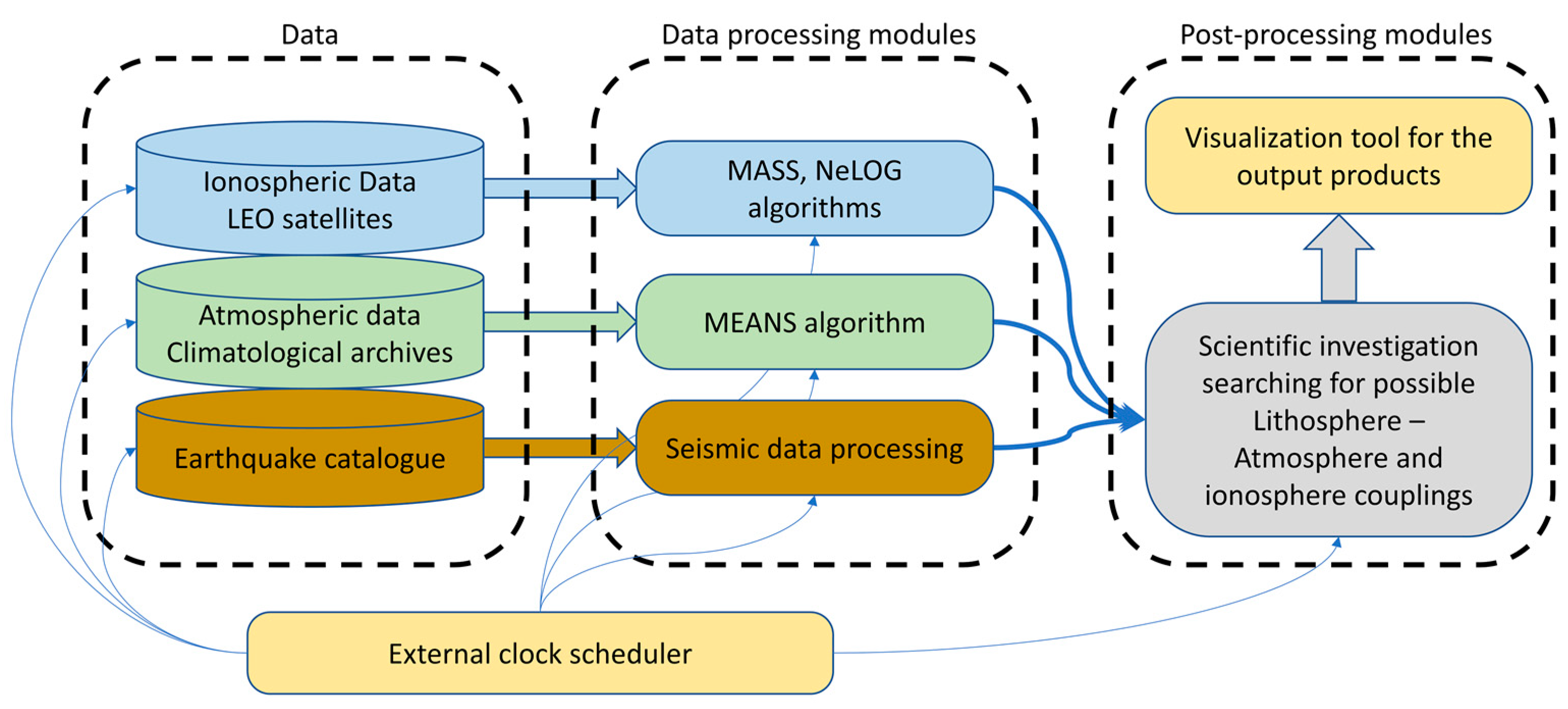
2. Materials and Methods
2.1. Earthquake Catalogue
2.2. Atmospheric Data Processing
2.3. Ionospheric Data Processing
3. Results
3.1. Seismological Investigation
3.2. Atmospheric Investigations
3.3. Ionospheric Investigations
4. Discussion and Conclusions
- The ML3.3 of 1 January 2023 is the mainshock of the seismic quiescence (R2-adj = 0.977 and acceleration coefficient C = 0.32);
- The mainshock, of magnitude M4.1 (R2-adj = 0.988 and acceleration coefficient C = 0.36), could be an incoming event in the following weeks/months.
Supplementary Materials
Author Contributions
Funding
Data Availability Statement
Acknowledgments
Conflicts of Interest
References
- Faccenna, C.; Soligo, M.; Billi, A.; De Filippis, L.; Funiciello, R.; Rossetti, C.; Tuccimei, P. Late Pleistocene Depositional Cycles of the Lapis Tiburtinus Travertine (Tivoli, Central Italy): Possible Influence of Climate and Fault Activity. Glob. Planet. Chang. 2008, 63, 299–308. [Google Scholar] [CrossRef]
- Frepoli, A.; Cimini, G.B.; De Gori, P.; De Luca, G.; Marchetti, A.; Monna, S.; Montuori, C.; Pagliuca, N.M. Seismic Sequences and Swarms in the Latium-Abruzzo-Molise Apennines (Central Italy): New Observations and Analysis from a Dense Monitoring of the Recent Activity. Tectonophysics 2017, 712–713, 312–329. [Google Scholar] [CrossRef]
- Utsu, T.; Ogata, Y.; Matsu’ura, S.R. The Centenary of the Omori Formula for a Decay Law of Aftershock Activity. J. Phys. Earth 1995, 43, 1–33. [Google Scholar] [CrossRef]
- ISIDe Working Group. Italian Seismological Instrumental and Parametric Database (ISIDe); Istituto Nazionale di Geofisica e Vulcanologia (INGV): Rome, Italy, 2007. [Google Scholar] [CrossRef]
- Chiaraluce, L.; Di Stefano, R.; Tinti, E.; Scognamiglio, L.; Michele, M.; Casarotti, E.; Cattaneo, M.; De Gori, P.; Chiarabba, C.; Monachesi, G.; et al. The 2016 Central Italy Seismic Sequence: A First Look at the Mainshocks, Aftershocks, and Source Models. Seismol. Res. Lett. 2017, 88, 757–771. [Google Scholar] [CrossRef]
- Wiemer, S. A Software Package to Analyse Seismicity: ZMAP. Seismol. Res. Lett. 2001, 72, 373–382. [Google Scholar] [CrossRef]
- Gutenberg, B. Seismicity of the Earth and Associated Phenomena; Read Books Ltd.: Worcestershire, UK, 2013. [Google Scholar]
- Montuori, C.; Murru, M.; Falcone, G. Spatial Variation of the B-Value Observed for the Periods Preceding and Following the 24 August 2016, Amatrice Earthquake (ML 6.0) (Central Italy). Ann. Geophys. 2016, 59, 12. [Google Scholar] [CrossRef]
- De Santis, A.; Cianchini, G.; Favali, P.; Beranzoli, L.; Boschi, E. The Gutenberg-Richter Law and Entropy of Earthquakes: Two Case Studies in Central Italy. Bull. Seismol. Soc. Am. 2011, 101, 1386–1395. [Google Scholar] [CrossRef]
- Mignan, A. The Stress Accumulation Model: Accelerating Moment Release and Seismic Hazard. In Advances in Geophysics; Elsevier: Amsterdam, The Netherlands, 2008; Volume 49, pp. 67–201. ISBN 978-0-12-374231-5. [Google Scholar]
- Dobrovolsky, I.P.; Zubkov, S.I.; Miachkin, V.I. Estimation of the Size of Earthquake Preparation Zones. Pure Appl. Geophys. 1979, 117, 1025–1044. [Google Scholar] [CrossRef]
- Mignan, A.; King, G.C.P.; Bowman, D. A Mathematical Formulation of Accelerating Moment Release Based on the Stress Accumulation Model. J. Geophys. Res. Solid Earth 2007, 112, B07308. [Google Scholar] [CrossRef] [Green Version]
- Cianchini, G.; De Santis, A.; Di Giovambattista, R.; Abbattista, C.; Amoruso, L.; Campuzano, S.A.; Carbone, M.; Cesaroni, C.; De Santis, A.; Marchetti, D.; et al. Revised Accelerated Moment Release Under Test: Fourteen Worldwide Real Case Studies in 2014–2018 and Simulations. Pure Appl. Geophys. 2020, 177, 4057–4087. [Google Scholar] [CrossRef]
- De Santis, A.; Cianchini, G.; Marchetti, D.; Piscini, A.; Sabbagh, D.; Perrone, L.; Campuzano, S.A.; Inan, S. A Multiparametric Approach to Study the Preparation Phase of the 2019 M7.1 Ridgecrest (California, United States) Earthquake. Front. Earth Sci. 2020, 8, 540398. [Google Scholar] [CrossRef]
- Piscini, A.; Marchetti, D.; De Santis, A. Multiparametric Climatological Analysis Associated with Global Significant Volcanic Eruptions During 2002–2017. Pure Appl. Geophys. 2019, 176, 3629–3647. [Google Scholar] [CrossRef]
- Marchetti, D.; de Santis, A.; D’Arcangelo, S.; Poggio, F.; Piscini, A.; Campuzano, S.A.; de Carvalho, W.V.J.O. Pre-Earthquake Chain Processes Detected from Ground to Satellite Altitude in Preparation of the 2016–2017 Seismic Sequence in Central Italy. Remote Sens. Environ. 2019, 229, 93–99. [Google Scholar] [CrossRef]
- Marchetti, D.; Zhu, K.; Zhang, H.; Zhima, Z.; Yan, R.; Shen, X.; Chen, W.; Cheng, Y.; He, X.; Wang, T.; et al. Clues of Lithosphere, Atmosphere and Ionosphere Variations Possibly Related to the Preparation of La Palma 19 September 2021 Volcano Eruption. Remote Sens. 2022, 14, 5001. [Google Scholar] [CrossRef]
- Akhoondzadeh, M.; De Santis, A.; Marchetti, D.; Wang, T. Developing a Deep Learning-Based Detector of Magnetic, Ne, Te and TEC Anomalies from Swarm Satellites: The Case of Mw 7.1 2021 Japan Earthquake. Remote Sens. 2022, 14, 1582. [Google Scholar] [CrossRef]
- Akhoondzadeh, M.; Marchetti, D. Developing a Fuzzy Inference System Based on Multi-Sensor Data to Predict Powerful Earthquake Parameters. Remote Sens. 2022, 14, 3203. [Google Scholar] [CrossRef]
- Marchetti, D.; de Santis, A.; Shen, X.; Campuzano, S.A.; Perrone, L.; Piscini, A.; Di Giovambattista, R.; Jin, S.; Ippolito, A.; Cianchini, G.; et al. Possible Lithosphere-Atmosphere-Ionosphere Coupling Effects Prior to the 2018 Mw = 7.5 Indonesia Earthquake from Seismic, Atmospheric and Ionospheric Data. J. Asian Earth Sci. 2020, 188, 104097. [Google Scholar] [CrossRef]
- Friis-Christensen, E.; Lühr, H.; Hulot, G. Swarm: A Constellation to Study the Earth’s Magnetic Field. Earth Planets Space 2006, 58, 351–358. [Google Scholar] [CrossRef]
- Akhoondzadeh, M.; De Santis, A.; Marchetti, D.; Piscini, A.; Cianchini, G. Multi Precursors Analysis Associated with the Powerful Ecuador (MW = 7.8) Earthquake of 16 April 2016 Using Swarm Satellites Data in Conjunction with Other Multi-Platform Satellite and Ground Data. Adv. Space Res. 2018, 61, 248–263. [Google Scholar] [CrossRef] [Green Version]
- Zhu, K.; Li, K.; Fan, M.; Chi, C.; Yu, Z. Precursor Analysis Associated With the Ecuador Earthquake Using Swarm A and C Satellite Magnetic Data Based on PCA. IEEE Access 2019, 7, 93927–93936. [Google Scholar] [CrossRef]
- Zhu, K.; Fan, M.; He, X.; Marchetti, D.; Li, K.; Yu, Z.; Chi, C.; Sun, H.; Cheng, Y. Analysis of Swarm Satellite Magnetic Field Data Before the 2016 Ecuador (Mw = 7.8) Earthquake Based on Non-Negative Matrix Factorization. Front. Earth Sci. 2021, 9, 621976. [Google Scholar] [CrossRef]
- Fan, M.; Zhu, K.; De Santis, A.; Marchetti, D.; Cianchini, G.; Piscini, A.; He, X.; Wen, J.; Wang, T.; Zhang, Y.; et al. Analysis of Swarm Satellite Magnetic Field Data for the 2015 Mw 7.8 Nepal Earthquake Based on Nonnegative Tensor Decomposition. IEEE Trans. Geosci. Remote Sens. 2022, 60, 2006119. [Google Scholar] [CrossRef]
- Ghamry, E.; Mohamed, E.K.; Sekertekin, A.; Fathy, A. Integration of Multiple Earthquakes Precursors before Large Earthquakes: A Case Study of 25 April 2015 in Nepal. J. Atmos. Sol. Terr. Phys. 2023, 242, 105982. [Google Scholar] [CrossRef]
- Marchetti, D.; De Santis, A.; Campuzano, S.A.; Soldani, M.; Piscini, A.; Sabbagh, D.; Cianchini, G.; Perrone, L.; Orlando, M. Swarm Satellite Magnetic Field Data Analysis Prior to 2019 Mw = 7.1 Ridgecrest (California, USA) Earthquake. Geosciences 2020, 10, 502. [Google Scholar] [CrossRef]
- De Santis, A.; Perrone, L.; Calcara, M.; Campuzano, S.A.; Cianchini, G.; D’Arcangelo, S.; Di Mauro, D.; Marchetti, D.; Nardi, A.; Orlando, M.; et al. A Comprehensive Multiparametric and Multilayer Approach to Study the Preparation Phase of Large Earthquakes from Ground to Space: The Case Study of the June 15 2019, M7.2 Kermadec Islands (New Zealand) Earthquake. Remote Sens. Environ. 2022, 283, 113325. [Google Scholar] [CrossRef]
- De Santis, A.; Marchetti, D.; Spogli, L.; Cianchini, G.; Pavón-Carrasco, F.J.; de Franceschi, G.; Di Giovambattista, R.; Perrone, L.; Qamili, E.; Cesaroni, C.; et al. Magnetic Field and Electron Density Data Analysis from Swarm Satellites Searching for Ionospheric Effects by Great Earthquakes: 12 Case Studies from 2014 to 2016. Atmosphere 2019, 10, 371. [Google Scholar] [CrossRef]
- Marchetti, D.; Akhoondzadeh, M. Analysis of Swarm Satellites Data Showing Seismo-Ionospheric Anomalies around the Time of the Strong Mexico (Mw = 8.2) Earthquake of 08 September 2017. Adv. Space Res. 2018, 62, 614–623. [Google Scholar] [CrossRef]
- Akhoondzadeh, M.; de Santis, A.; Marchetti, D.; Shen, X. Swarm-TEC Satellite Measurements as a Potential Earthquake Precursor Together With Other Swarm and CSES Data: The Case of Mw7.6 2019 Papua New Guinea Seismic Event. Front. Earth Sci. 2022, 10, 820189. [Google Scholar] [CrossRef]
- Christodoulou, V.; Bi, Y.; Wilkie, G. A Tool for Swarm Satellite Data Analysis and Anomaly Detection. PLoS ONE 2019, 14, e0212098. [Google Scholar] [CrossRef]
- de Santis, A.; Balasis, G.; Pavón-Carrasco, F.J.; Cianchini, G.; Mandea, M. Potential Earthquake Precursory Pattern from Space: The 2015 Nepal Event as Seen by Magnetic Swarm Satellites. Earth Planet. Sci. Lett. 2017, 461, 119–126. [Google Scholar] [CrossRef]
- de Santis, A.; Marchetti, D.; Pavón-Carrasco, F.J.; Cianchini, G.; Perrone, L.; Abbattista, C.; Alfonsi, L.; Amoruso, L.; Campuzano, S.A.; Carbone, M.; et al. Precursory Worldwide Signatures of Earthquake Occurrences on Swarm Satellite Data. Sci. Rep. 2019, 9, 20287. [Google Scholar] [CrossRef]
- Marchetti, D.; De Santis, A.; Campuzano, S.A.; Zhu, K.; Soldani, M.; D’Arcangelo, S.; Orlando, M.; Wang, T.; Cianchini, G.; Di Mauro, D.; et al. Worldwide Statistical Correlation of Eight Years of Swarm Satellite Data with M5.5+ Earthquakes: New Hints about the Preseismic Phenomena from Space. Remote Sens. 2022, 14, 2649. [Google Scholar] [CrossRef]
- Xiong, P.; Marchetti, D.; De Santis, A.; Zhang, X.; Shen, X. SafeNet: SwArm for Earthquake Perturbations Identification Using Deep Learning Networks. Remote Sens. 2021, 13, 5033. [Google Scholar] [CrossRef]
- Sasmal, S.; Chowdhury, S.; Kundu, S.; Politis, D.Z.; Potirakis, S.M.; Balasis, G.; Hayakawa, M.; Chakrabarti, S.K. Pre-Seismic Irregularities during the 2020 Samos (Greece) Earthquake (M = 6.9) as Investigated from Multi-Parameter Approach by Ground and Space-Based Techniques. Atmosphere 2021, 12, 1059. [Google Scholar] [CrossRef]
- Piscini, A.; de Santis, A.; Marchetti, D.; Cianchini, G. A Multiparametric Climatological Approach to Study the 2016 Amatrice–Norcia (Central Italy) Earthquake Preparatory Phase. Pure Appl. Geophys. 2017, 174, 3673–3688. [Google Scholar] [CrossRef]
- Allard, P.; Carbonnelle, J.; Métrich, N.; Loyer, H.; Zettwoog, P. Sulphur Output and Magma Degassing Budget of Stromboli Volcano. Nature 1994, 368, 326–330. [Google Scholar] [CrossRef]
- Pulinets, S.; Ouzounov, D. Lithosphere–Atmosphere–Ionosphere Coupling (LAIC) Model—An Unified Concept for Earthquake Precursors Validation. J. Asian Earth Sci. 2011, 41, 371–382. [Google Scholar] [CrossRef]
- Freund, F. Pre-Earthquake Signals: Underlying Physical Processes. J. Asian Earth Sci. 2011, 41, 383–400. [Google Scholar] [CrossRef]
- Marchetti, D.; De Santis, A.; D’Arcangelo, S.; Poggio, F.; Jin, S.; Piscini, A.; Campuzano, S.A. Magnetic Field and Electron Density Anomalies from Swarm Satellites Preceding the Major Earthquakes of the 2016–2017 Amatrice-Norcia (Central Italy) Seismic Sequence. Pure Appl. Geophys. 2020, 177, 305–319. [Google Scholar] [CrossRef]
- Lang, T. Non-Quality Controlled Lightning Imaging Sensor (LIS) on International Space Station (ISS) Science Data; NASA Global Hydrology Resource Center DAAC: Huntsville, AL, USA, 2022. [Google Scholar] [CrossRef]
- Kuo, C.L.; Lee, L.C.; Huba, J.D. An Improved Coupling Model for the Lithosphere-Atmosphere-Ionosphere System. J. Geophys. Res. Space Phys. 2014, 119, 3189–3205. [Google Scholar] [CrossRef]
- Perevalova, N.P.; Sankov, V.A.; Astafyeva, E.I.; Zhupityaeva, A.S. Threshold Magnitude for Ionospheric TEC Response to Earthquakes. J. Atmos. Sol. Terr. Phys. 2014, 108, 77–90. [Google Scholar] [CrossRef]
- Wu, L.; Qi, Y.; Mao, W.; Lu, J.; Ding, Y.; Peng, B.; Xie, B. Scrutinizing and Rooting the Multiple Anomalies of Nepal Earthquake Sequence in 2015 with the Deviation–Time–Space Criterion and Homologous Lithosphere–Coversphere–Atmosphere–Ionosphere Coupling Physics. Nat. Hazards Earth Syst. Sci. 2023, 23, 231–249. [Google Scholar] [CrossRef]
- Marchetti, D.; Zhu, K.; Marchetti, L.; Zhang, Y.; Chen, W.; Cheng, Y.; Fan, M.; Wang, S.; Wang, T.; Wen, J.; et al. Quick Report of the ML = 3.3 on 1 January 2023 Guidonia (Rome, Italy) Earthquake: Evidence of a Seismic Acceleration. Preprints 2023, 2023010067. [Google Scholar] [CrossRef]


| Estimated Magnitude | Dobrovolsky Radius [km] | b-Value (In Previous 6 Months) | C 1 (In the Previous 6 Months) | |
|---|---|---|---|---|
| Real earthquake | 3.3 | 26.2 | 1.0 ± 0.3 | 0.318 |
| Tested earthquakes | 3.5 | 32.0 | 1.0 ± 0.3 | 0.359 |
| 3.7 | 39.0 | 0.7 ± 0.1 | 0.342 | |
| 3.9 | 47.5 | 0.7 ± 0.1 | 0.326 | |
| 4.1 | 57.9 | 0.7 ± 0.1 | 0.356 | |
| 4.3 | 70.6 | 1.0 ± 0.2 | 0.714 | |
| 4.5 | 86.1 | 1.04 ± 0.05 | 0.943 | |
| 4.7 | 105.0 | 1.15 ± 0.03 | 1.075 |
| Date | Atmospheric Parameter | |||||
|---|---|---|---|---|---|---|
| Surface Air Temperature | Surface Specific Humidity | Aerosol | SO2 | Surface Total Energy Latent Heat Flux | Total Precipitation | |
| 4 July 2022 | X | |||||
| 7 July 2022 | X | |||||
| 8 July 2022 | X | |||||
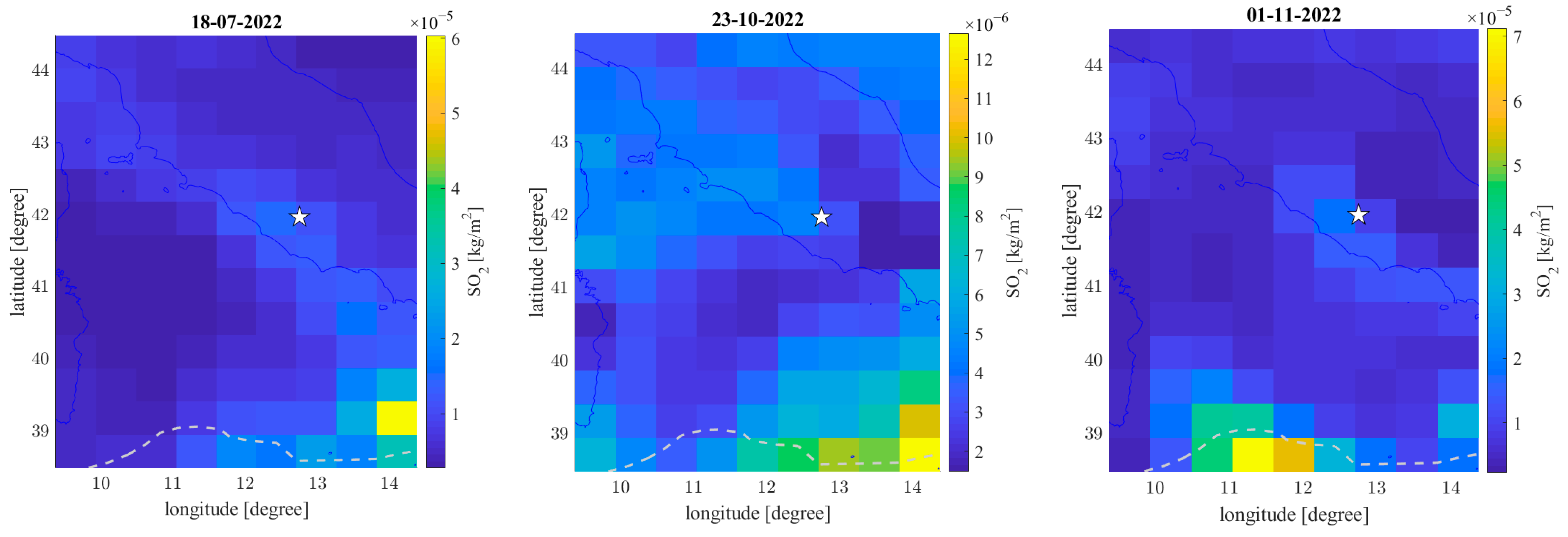
| 18 July 2022 | X | |||||
| 20 July 2022 | X | |||||
| 17 August 2022 | X | |||||
| 18 August 2022 | X | X | ||||
| 19 August 2022 | X | |||||
| 31 August 2022 | X | |||||
| 8 September 2022 | X | X | ||||
| 15 September 2022 | X | |||||
| 17 September 2022 | X | X | ||||
| 21 September 2022 | X | X | ||||
| 22 September 2022 | X | |||||
| 27 September 2022 | X | |||||
| 8 October 2022 | X | |||||
| 10 October 2022 | X | |||||
| 23 October 2022 | X | |||||
| 1 November 2022 | X | |||||
| 5 November 2022 | X | |||||
| 13 November 2022 | X | |||||
| 22 November 2022 | X | |||||
| 25 November 2022 | X | |||||
| 2 December 2022 | X | |||||
| 3 December 2022 | X | X | ||||
| Swarm | Date | Time UT | Local Time | Anomalous Component | Dst [nT] | ap [nT] | F10.7 [SFU] | Figure |
|---|---|---|---|---|---|---|---|---|
| Bravo | 9 July 2022 | 19:25:45 | 20:19:32 | X-North, Y-East, Z-Center | −15 | 6 | 139.9 | Figure S9 |
| Bravo | 10 July 2022 | 07:38:42 | 08:33:08 | X-North, Y-East, Z-Center | −6 | 9 | 155.3 | Figure S10 |
| Bravo | 16 July 2022 | 18:51:07 | 19:43:40 | X-North, Y-East, Z-Center | −7 | 3 | 176.9 | Figure S11 |
| Bravo | 17 July 2022 | 07:04:03 | 07:57:16 | X-North | −8 | 3 | 163.7 | Figure S12 |
| Bravo | 31 July 2022 | 05:54:17 | 06:45:33 | Y-East | 14 | 5 | 95.1 | Figure S13 |
| Bravo | 6 August 2022 | 17:06:22 | 17:56:06 | Y-East | 20 | 3 | 116.2 | Figure 9 |
| Bravo | 14 August 2022 | 04:44:07 | 05:33:49 | X-North | −20 | 7 | 125.7 | Figure S14 |
| Charlie | 26 August 2022 | 14:18:41 | 15:05:31 | Y-East | 1 | 4 | 120.4 | Figure S15 |
| Alpha | 30 August 2022 | 13:53:05 | 14:46:46 | X-North | −4 | 7 | 124.4 | Figure S16 |
| Charlie | 26 September 2022 | 11:19:43 | 12:19:28 | X-North, Y-East, Z-Center | 2 | 4 | 135.7 | Figure S17 |
| Alpha | 3 October 2022 | 10:56:32 | 11:44:51 | Y-East | −11 | 5 | 158.3 | Figure S18 |
| Charlie | 26 October 2022 | 08:42:02 | 09:38:43 | X-North | 10 | 0 | 122.8 | Figure S19 |
| Alpha, Charlie | 13 November 2022 | 18:44:39 | 19:43:53 | X-North, Y-East, Z-Center | −8 | 6 | 136.1 | Figure 10 and Figure S20 |
| Alpha | 16 November 2022 | 18:46:36 | 19:27:45 | Y-East | 5 | 5 | 131.5 | Figure S21 |
| Bravo | 8 December 2022 | 18:50:27 | 19:34:44 | X-North, Y-East | −14 | 7 | 142.3 | Figure S22 |
| Alpha | 16 December 2022 | 15:54:40 | 16:47:10 | Y-East | −1 | 2 | 164.0 | Figure 11 |
Disclaimer/Publisher’s Note: The statements, opinions and data contained in all publications are solely those of the individual author(s) and contributor(s) and not of MDPI and/or the editor(s). MDPI and/or the editor(s) disclaim responsibility for any injury to people or property resulting from any ideas, methods, instructions or products referred to in the content. |
© 2023 by the authors. Licensee MDPI, Basel, Switzerland. This article is an open access article distributed under the terms and conditions of the Creative Commons Attribution (CC BY) license (https://creativecommons.org/licenses/by/4.0/).
Share and Cite
Marchetti, D.; Zhu, K.; Marchetti, L.; Zhang, Y.; Chen, W.; Cheng, Y.; Fan, M.; Wang, S.; Wang, T.; Wen, J.; et al. Quick Report on the ML = 3.3 on 1 January 2023 Guidonia (Rome, Italy) Earthquake: Evidence of a Seismic Acceleration. Remote Sens. 2023, 15, 942. https://doi.org/10.3390/rs15040942
Marchetti D, Zhu K, Marchetti L, Zhang Y, Chen W, Cheng Y, Fan M, Wang S, Wang T, Wen J, et al. Quick Report on the ML = 3.3 on 1 January 2023 Guidonia (Rome, Italy) Earthquake: Evidence of a Seismic Acceleration. Remote Sensing. 2023; 15(4):942. https://doi.org/10.3390/rs15040942
Chicago/Turabian StyleMarchetti, Dedalo, Kaiguang Zhu, Laura Marchetti, Yiqun Zhang, Wenqi Chen, Yuqi Cheng, Mengxuan Fan, Siyu Wang, Ting Wang, Jiami Wen, and et al. 2023. "Quick Report on the ML = 3.3 on 1 January 2023 Guidonia (Rome, Italy) Earthquake: Evidence of a Seismic Acceleration" Remote Sensing 15, no. 4: 942. https://doi.org/10.3390/rs15040942