
Pre-Seismic Anomaly Detection from Multichannel Infrared Images of FY-4A Satellite

Abstract
:1. Introduction
2. Materials and Methods
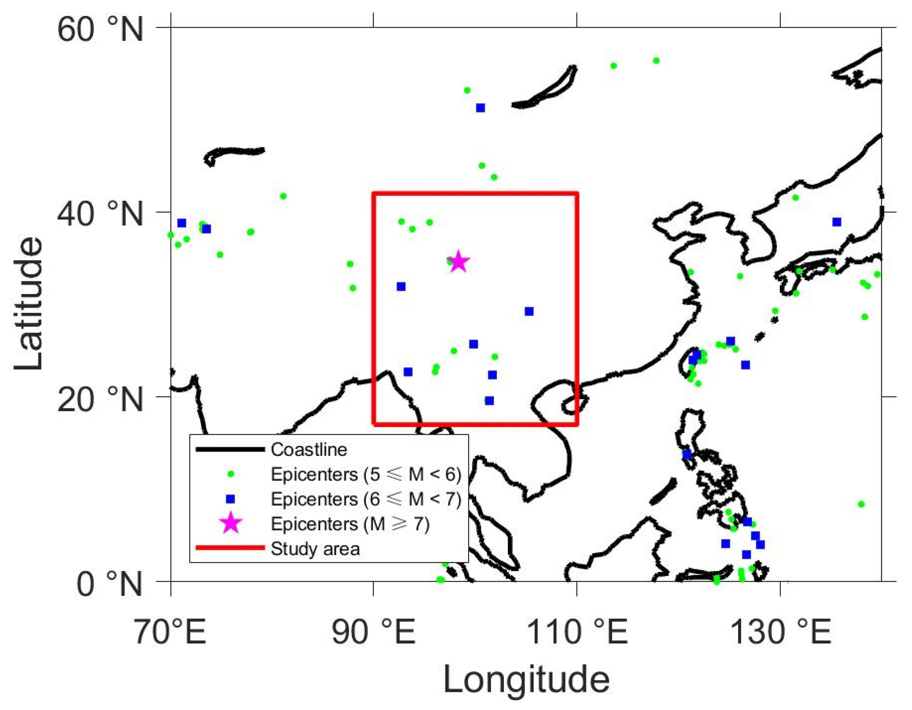
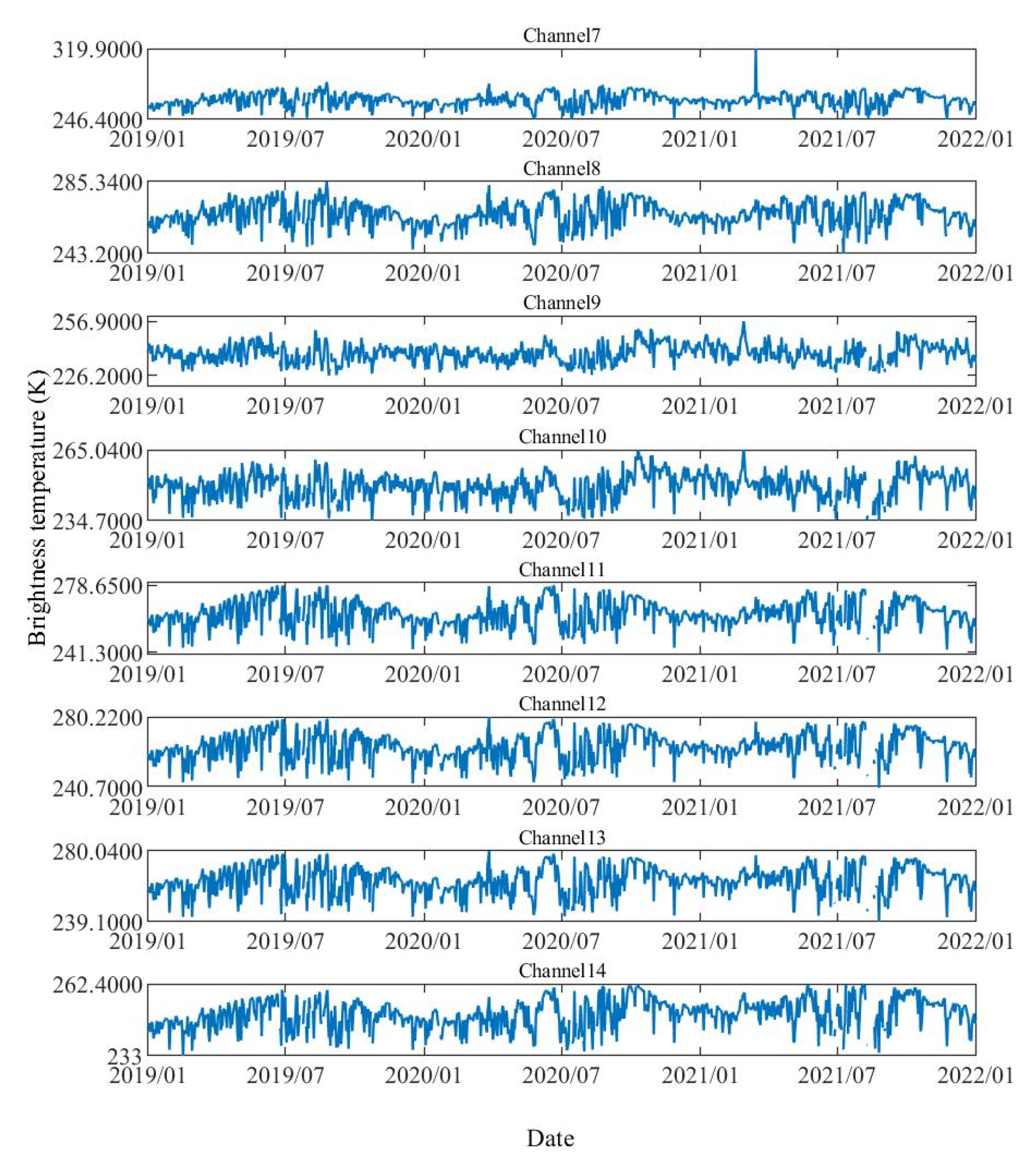
2.1. Data and Study Area
2.2. Anomaly Detection
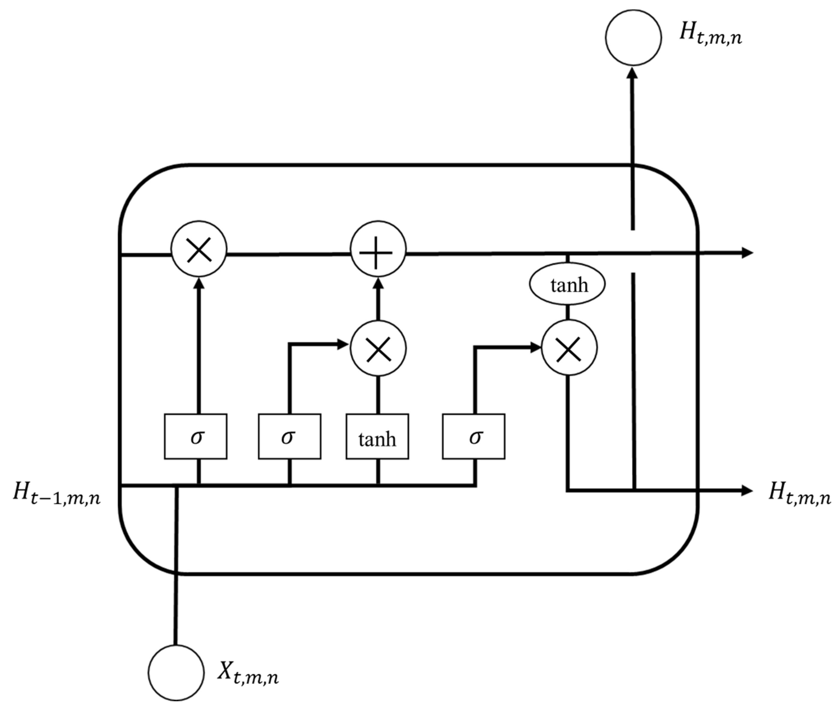
2.2.1. Long Short-Term Memory (LSTM)
2.2.2. Density-Based Spatial Clustering of Application with Noise (DBSCAN)
2.3. Statistical Method
3. Results
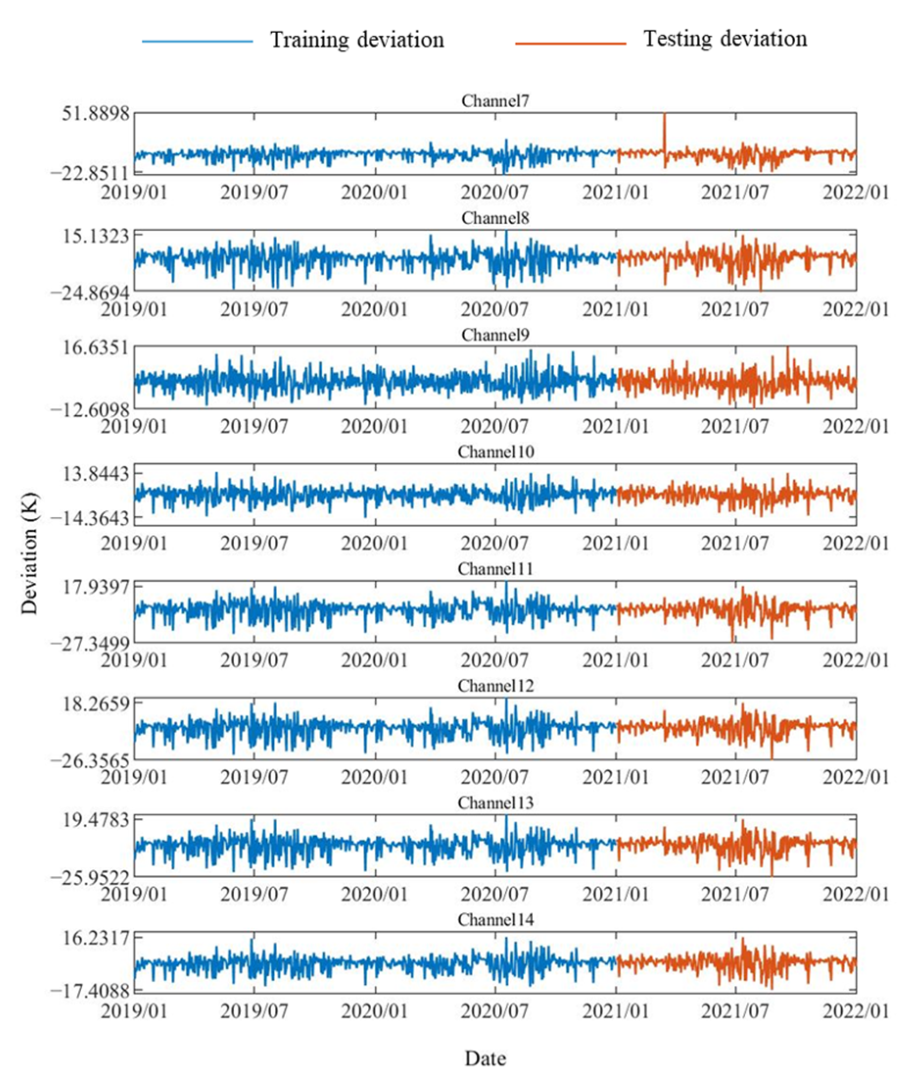
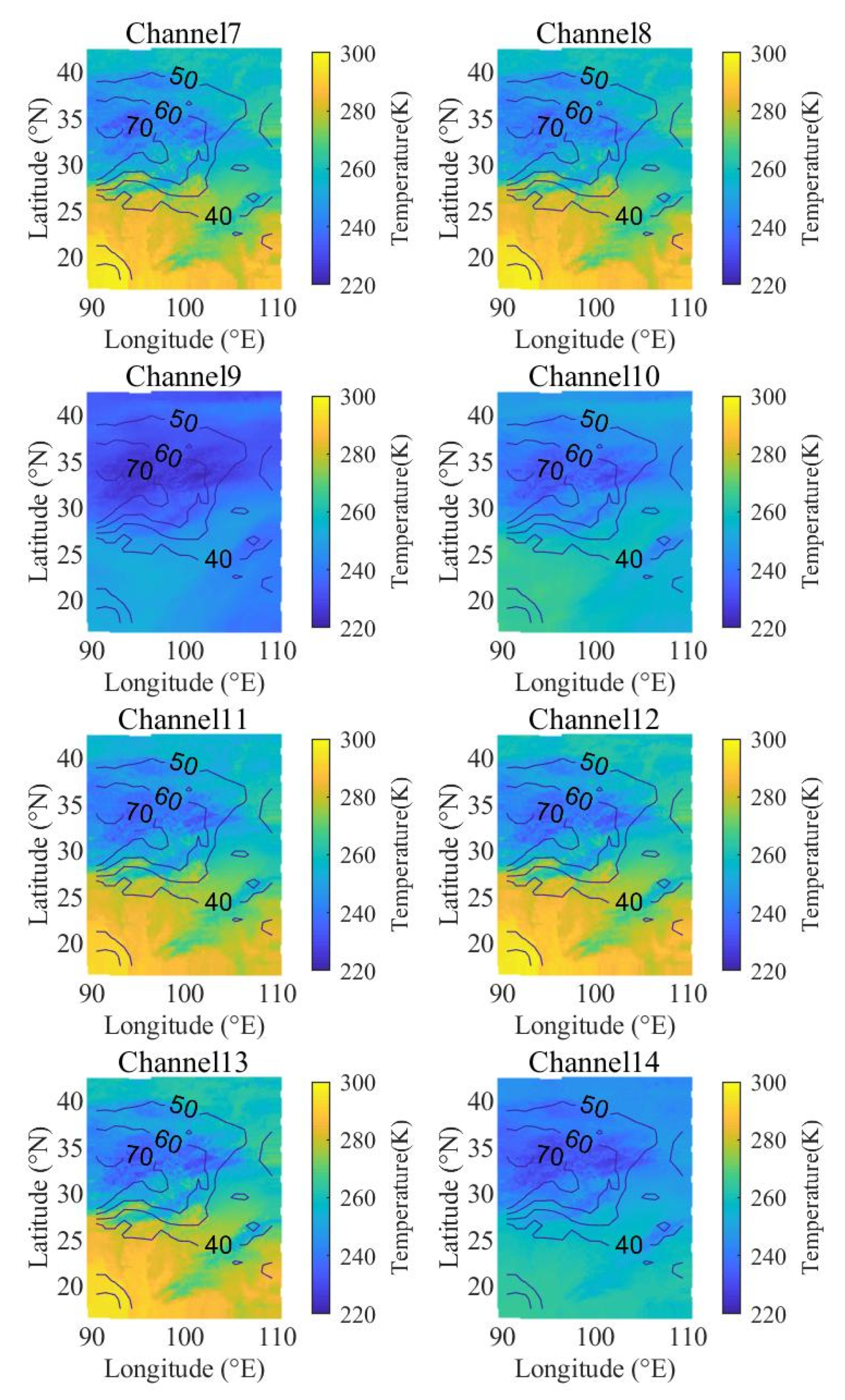
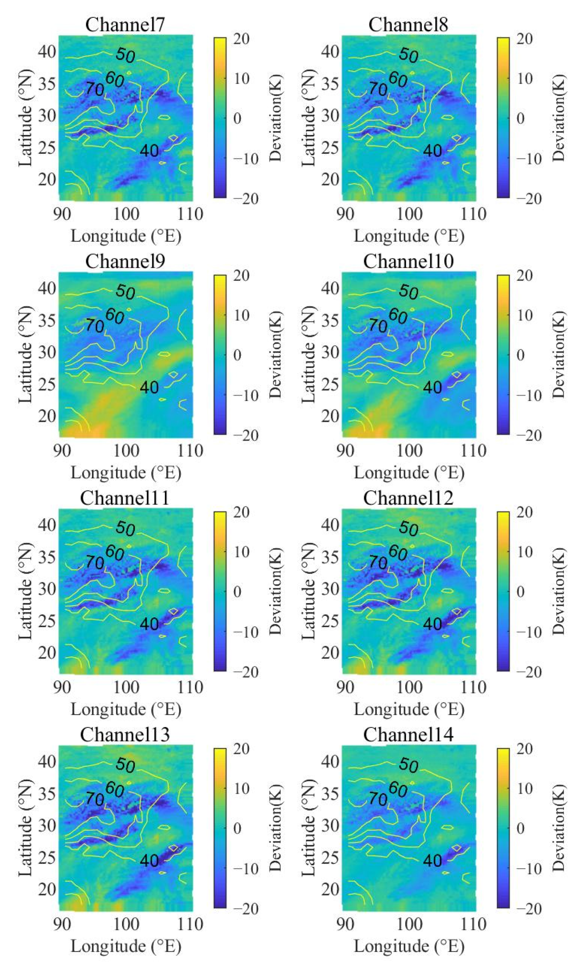
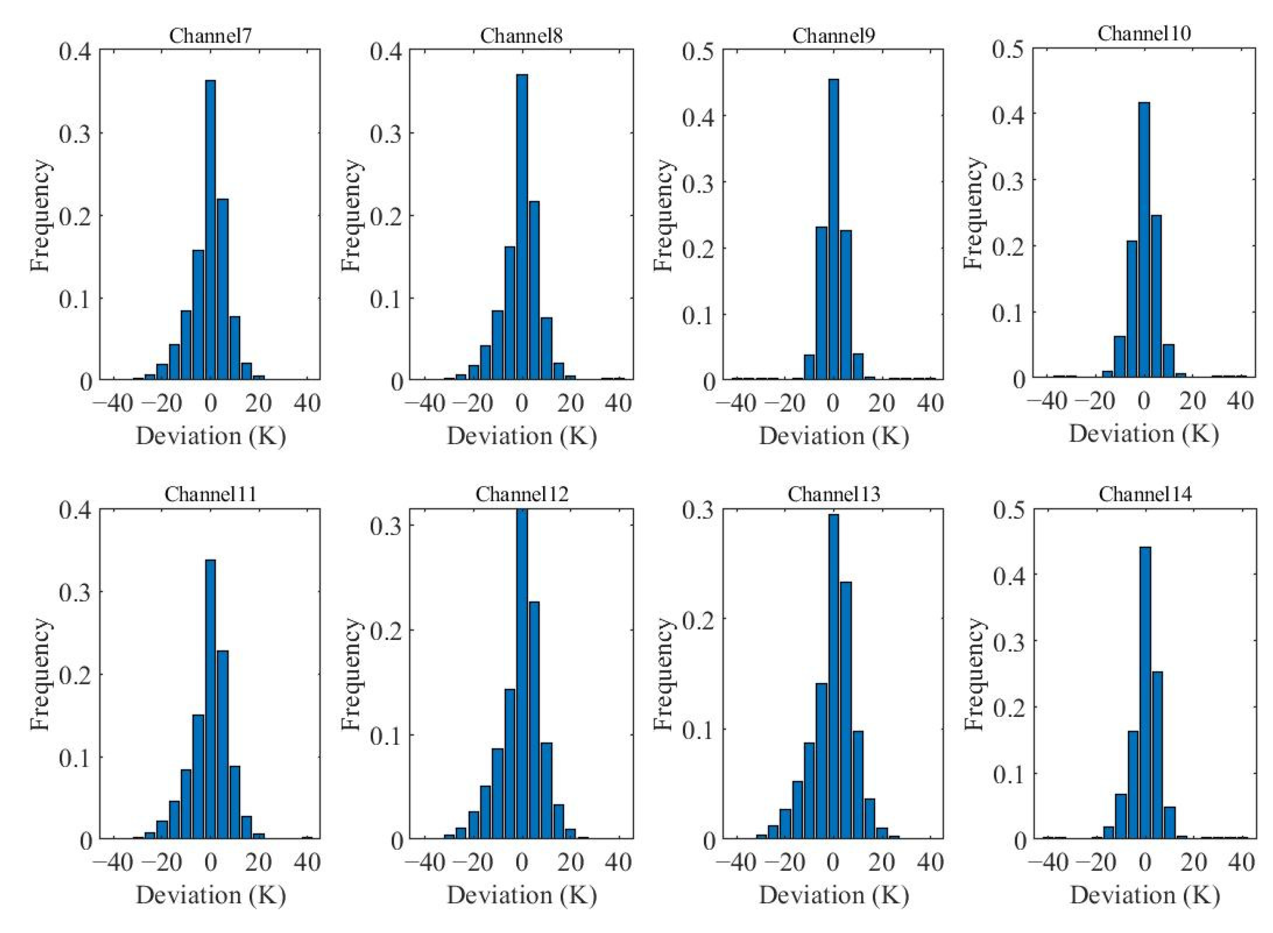
3.1. The Deviation of the LSTM Model
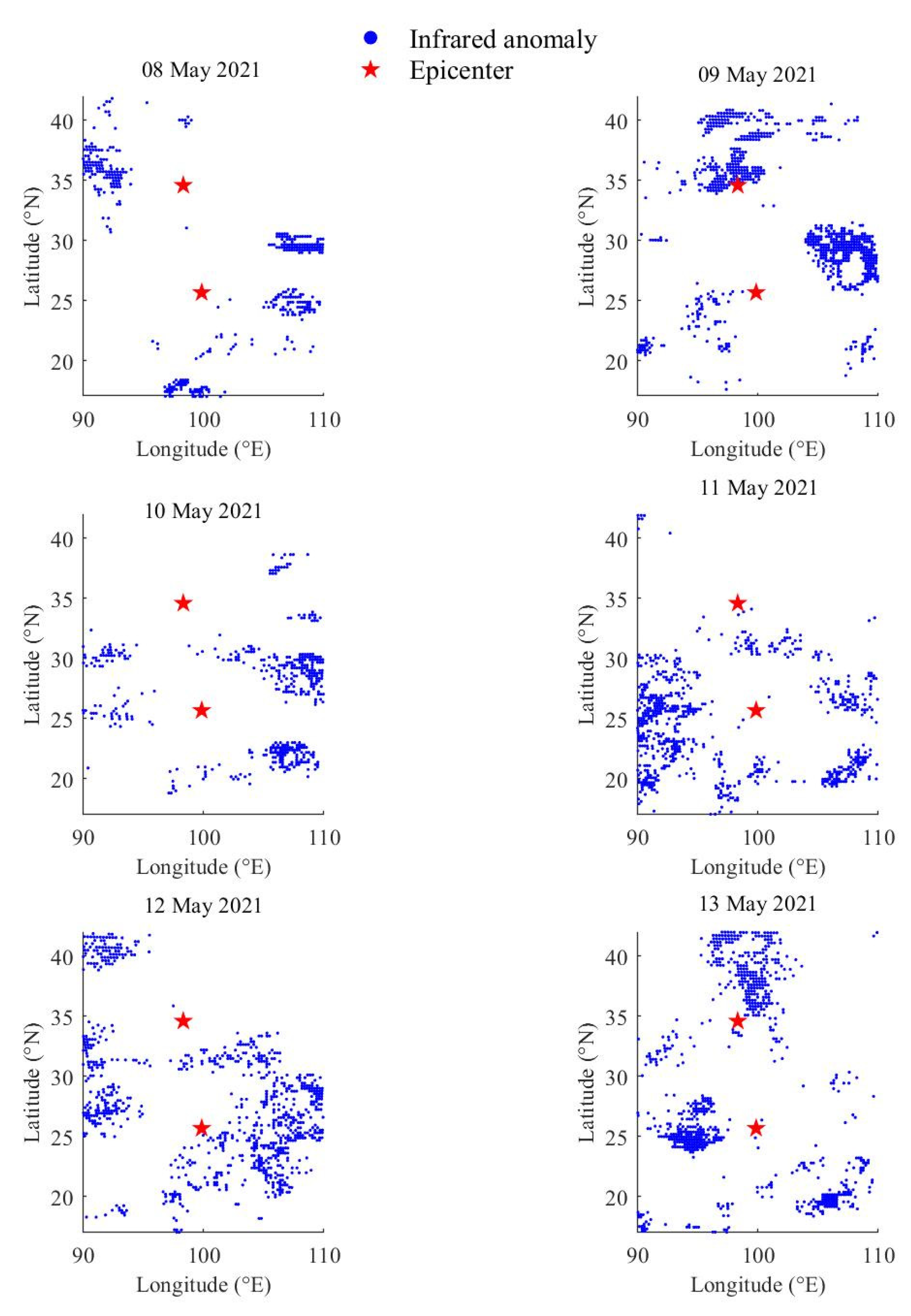
3.2. Clustering Results
3.3. Statistical Results
4. Discussion
5. Conclusions
Supplementary Materials
Author Contributions
Funding
Institutional Review Board Statement
Informed Consent Statement
Data Availability Statement
Acknowledgments
Conflicts of Interest
References
- Varotsos, P.A.; Sarlis, N.V.; Skordas, E.S. Self-organized criticality and earthquake predictability: A long-standing question in the light of natural time analysis. EPL (Europhys. Lett.) 2020, 132, 29001. [Google Scholar] [CrossRef]
- De Santis, A.; Perrone, L.; Calcara, M.; Campuzano, S.; Cianchini, G.; D’Arcangelo, S.; Di Mauro, D.; Marchetti, D.; Nardi, A.; Orlando, M.; et al. A comprehensive multiparametric and multilayer approach to study the preparation phase of large earthquakes from ground to space: The case study of the June 15 2019, M7.2 Kermadec Islands earthquake. Remote Sens. Environ. 2022, 283, 113325. [Google Scholar] [CrossRef]
- Gu, G. Advantages of GNSS in Monitoring Crustal Deformation for Detection of Precursors to Strong Earthquakes. Positioning 2013, 4, 11–19. [Google Scholar] [CrossRef] [Green Version]
- Wei, C.; Zhang, Y.; Guo, X.; Hui, S.; Qin, M.; Zhang, Y. Thermal Infrared Anomalies of Several Strong Earthquakes. Sci. World J. 2013, 2013, 208407. [Google Scholar] [CrossRef] [Green Version]
- Bhardwaj, A.; Singh, S.; Sam, L.; Joshi, P.K.; Bhardwaj, A.; Martín-Torres, F.J.; Kumar, R. A review on remotely sensed land surface temperature anomaly as an earthquake precursor. Int. J. Appl. Earth Obs. Geoinf. 2017, 63, 158–166. [Google Scholar] [CrossRef]
- Zhang, L.; Jiang, M.; Jing, F. Sea temperature variation associated with the 2021 Haiti Mw 7.2 earthquake and possible mechanism. Geomat. Nat. Hazards Risk 2022, 13, 2840–2863. [Google Scholar] [CrossRef]
- Jing, F.; Shen, X.H.; Kang, C.L.; Xiong, P. Variations of multi-parameter observations in atmosphere related to earthquake. Nat. Hazards Earth Syst. Sci. 2013, 13, 27–33. [Google Scholar] [CrossRef] [Green Version]
- Bao, Z.; Zhao, J.; Huang, P.; Yong, S.; Wang, X. A Deep Learning-Based Electromagnetic Signal for Earthquake Magnitude Prediction. Sensors 2021, 21, 4434. [Google Scholar] [CrossRef]
- Uyeda, S.; Nagao, T.; Kamogawa, M. Short-term earthquake prediction: Current status of seismo-electromagnetics. Tectonophysics 2009, 470, 205–213. [Google Scholar] [CrossRef]
- Adil, M.; Şentürk, E.; Pulinets, S.; Amory-Mazaudier, C. A Lithosphere–Atmosphere–Ionosphere Coupling Phenomenon Observed before M 7.7 Jamaica Earthquake. Pure Appl. Geophys. 2021, 178, 3869–3886. [Google Scholar] [CrossRef]
- Huang, Q. Seismicity Pattern Changes Prior to the 2008 Ms7.3 Yutian Earthquake. Entropy 2019, 21, 118. [Google Scholar] [CrossRef] [PubMed] [Green Version]
- Saraf, A.; Rawat, V.; Choudhury, S.; Dasgupta, S.; Das, J. Advances in understanding of the mechanism for generation of earthquake thermal precursors detected by satellites. Int. J. Appl. Earth Obs. Geoinf. 2009, 11, 373–379. [Google Scholar] [CrossRef]
- Guo, Z.; Qiang, S.; Wang, C.; Liu, Z.; Gao, X.; Zhang, W.; Yu, Y.; Zhang, H.; Qiu, J. The mechanism of earthquake’s thermal infrared radiation precursory on remote sensing images. In Proceedings of the IEEE International Geoscience and Remote Sensing Symposium, Toronto, ON, Canada, 24–28 June 2002; Volume 4, pp. 2036–2038. [Google Scholar] [CrossRef]
- Qiang, Z.J.; Kong, L.C.; Zheng, L.Z.; Guo, M.-H.; Wang, G.-P.; Zhao, Y. An experimental study on temperature increasing mechanism of satellitic thermo-infrared. Acta Seismol. Sin. 1997, 10, 247–252. [Google Scholar] [CrossRef]
- Jiao, Z.-H.; Zhao, J.; Shan, X. Pre-seismic anomalies from optical satellite observations: A review. Nat. Hazards Earth Syst. Sci. 2018, 18, 1013–1036. [Google Scholar] [CrossRef] [Green Version]
- Genzano, N.; Filizzola, C.; Hattori, K.; Pergola, N.; Tramutoli, V. Statistical Correlation Analysis between Thermal Infrared Anomalies Observed from MTSATs and Large Earthquakes Occurred in Japan (2005–2015). J. Geophys. Res. Solid Earth 2021, 126, e2020JB020108. [Google Scholar] [CrossRef]
- Pulinets, S.; Ouzounov, D. Lithosphere–Atmosphere–Ionosphere Coupling (LAIC) model—An unified concept for earthquake precursors validation. J. Asian Earth Sci. 2010, 41, 371–382. [Google Scholar] [CrossRef]
- Venkatachalapathy, H.; Sreedharan, V.; Venkatanathan, N. Observation of Earthquake Precursors—A Study on OLR Scenario Prior to the Earthquakes of Indian and Neighboring Region Occurred in 2016. Int. J. Earth Sci. Eng. 2016, 9, 264–268. [Google Scholar]
- Dong, N.; Liao, H. Characteristics of Thermal Infrared Anomalies during the Earthquakes in Wenchuan, Lushan in Ya’an and Jiuzhaigou. IOP Conf. Ser. Earth Environ. Sci. 2021, 783, 012132. [Google Scholar] [CrossRef]
- Akhoondzadeh, M.; De Santis, A.; Marchetti, D.; Piscini, A.; Cianchini, G. Multi precursors analysis associated with the powerful Ecuador (MW = 7.8) earthquake of 16 April 2016 using Swarm satellites data in conjunction with other multi-platform satellite and ground data. Adv. Space Res. 2017, 61, 248–263. [Google Scholar] [CrossRef] [Green Version]
- Zhang, X.; Zhang, Y.; Guo, X.; Wei, C.; Zhang, L. Analysis of thermal infrared anomaly in the Nepal MS 8.1 earthquake. Earth Sci. Front. 2017, 24, 227–233. [Google Scholar] [CrossRef]
- Yao, Q.-L.; Qiang, Z.-J. Thermal infrared anomalies as a precursor of strong earthquakes in the distant future. Nat. Hazards 2012, 62, 991–1003. [Google Scholar] [CrossRef]
- Sun, D.; Zheng, H. Simulation Study of Infrared Transmittance under Different Atmospheric Conditions. J. Phys. Conf. Ser. 2022, 2356, 012045. [Google Scholar] [CrossRef]
- Carolina, F.; Pergola, N.; Pietrapertosa, C.; Valerio, T. Robust satellite techniques for seismically active areas monitoring: A sensitivity analysis on September 7, 1999 Athens’s earthquake. Phys. Chem. Earth 2004, 29, 517–527. [Google Scholar] [CrossRef]
- Valerio, T.; Aliano, C.; Corrado, R.; Carolina, F.; Genzano, N.; Lisi, M.; Martinelli, G.; Pergola, N. On the possible origin of thermal infrared radiation (TIR) anomalies in earthquake-prone areas observed using robust satellite techniques (RST). Chem. Geol. 2013, 339, 157–168. [Google Scholar] [CrossRef]
- Xie, T.; Kang, C.; Ma, W. Thermal infrared brightness temperature anomalies associated with the Yushu (China) Ms = 7.1 earthquake on 14 April 2010. Nat. Hazards Earth Syst. Sci. 2013, 13, 1105–1111. [Google Scholar] [CrossRef] [Green Version]
- Akhoondzadeh, M. A comparison of classical and intelligent methods to detect potential thermal anomalies before the 11 August 2012 Varzeghan, Iran, earthquake (Mw = 6.4). Nat. Hazards Earth Syst. Sci. 2013, 13, 1077–1083. [Google Scholar] [CrossRef]
- Saradjian, M.R.; Akhoondzadeh, M. Thermal anomalies detection before strong earthquakes (M > 6.0) using interquartile, wavelet and Kalman filter methods. Nat. Hazards Earth Syst. Sci. 2011, 11, 1099–1108. [Google Scholar] [CrossRef]
- Akhoondzadeh, M. A MLP neural network as an investigator of TEC time series to detect seismo-ionospheric anomalies. Adv. Space Res. 2013, 51, 2048–2057. [Google Scholar] [CrossRef]
- Akhoondzadeh, M. Support vector machines for TEC seismo-ionospheric anomalies detection. Ann. Geophys. 2013, 31, 173–186. [Google Scholar] [CrossRef] [Green Version]
- Akhoondzadeh, M. Genetic algorithm for TEC seismo-ionospheric anomalies detection around the time of the Solomon (Mw = 8.0) earthquake of 6 February 2013. Adv. Space Res. 2013, 52, 581–590. [Google Scholar] [CrossRef]
- Zhai, D.; Zhang, X.; Xiong, P. Detecting Thermal Anomalies of Earthquake Process within Outgoing Longwave Radiation Using Time Series Forecasting Models. Ann. Geophys. 2020, 63, PA548. [Google Scholar] [CrossRef]
- Jing, F.; Zhang, L.; Singh, R. Pronounced Changes in Thermal Signals Associated with the Madoi (China) M 7.3 Earthquake from Passive Microwave and Infrared Satellite Data. Remote Sens. 2022, 14, 2539. [Google Scholar] [CrossRef]
- Yang, X.; Zhang, T.-B.; Lu, Q.; Long, F.; Liang, M.-J.; Wu, W.-W.; Gong, Y.; Wei, J.-X.; Wu, J. Variation of Thermal Infrared Brightness Temperature Anomalies in the Madoi Earthquake and Associated Earthquakes in the Qinghai-Tibetan Plateau (China). Front. Earth Sci. 2022, 10, 823540. [Google Scholar] [CrossRef]
- Guo, X.; Zhang, Y.-S.; Wei, C.-X.; Zhong, M.-J.; Zhang, X. Medium Wave Infrared Brightness Anomalies of Wenchuan 8.0 and Zhongba 6.8 Earthquakes. Acta Geosci. Sin. 2014, 35, 338–344. [Google Scholar] [CrossRef]
- Zhang, P.; Zhu, L.; Tang, S.; Gao, L.; Chen, L.; Zheng, W.; Han, X.; Chen, J.; Shao, J. General Comparison of FY-4A/AGRI With Other GEO/LEO Instruments and Its Potential and Challenges in Non-meteorological Applications. Front. Earth Sci. 2019, 6, 224. [Google Scholar] [CrossRef] [Green Version]
- Tramutoli, V.; Corrado, R.; Filizzola, C.; Genzano, N.; Lisi, M.; Pergola, N. From visual comparison to Robust Satellite Techniques: 30 years of thermal infrared satellite data analyses for the study of earthquake preparation phases. Boll. Geofis. Teor. Appl. 2015, 56, 167–202. [Google Scholar]
- Yu, Y.; Si, X.; Hu, C.; Zhang, J. A Review of Recurrent Neural Networks: LSTM Cells and Network Architectures. Neural Comput. 2019, 31, 1235–1270. [Google Scholar] [CrossRef]
- Hafeez, A.; Shah, M.; Shahzad, R. Machine Learning Based Thermal Anomaly Detection Associated with Three Earthquakes in Pakistan Using MODIS LST. In Proceedings of the 2021 Seventh International Conference on Aerospace Science and Engineering (ICASE), Islamabad, Pakistan, 14–16 December 2021; pp. 1–5. [Google Scholar] [CrossRef]
- Schubert, E.; Sander, J.; Ester, M.; Kriegel, H.; Xu, X. DBSCAN revisited, revisited: Why and how you should (still) use DBSCAN. ACM Trans. Database Syst. (TODS) 2017, 42, 19. [Google Scholar] [CrossRef]
- Piscini, A.; De Santis, A.; Marchetti, D.; Cianchini, G. A Multi-parametric Climatological Approach to Study the 2016 Amatrice–Norcia (Central Italy) Earthquake Preparatory Phase. Pure Appl. Geophys. 2017, 174, 3673–3688. [Google Scholar] [CrossRef]
- Zhang, Y.; Meng, Q. A statistical analysis of TIR anomalies extracted by RSTs in relation to an earthquake in the Sichuan area using MODIS LST data. Nat. Hazards Earth Syst. Sci. 2019, 19, 535–549. [Google Scholar] [CrossRef]
- Shebalin, P.N.; Narteau, C.; Zechar, J.D.; Holschneider, M. Combining earthquake forecasts using differential probability gains. Earth Planet Sp. 2014, 66, 37. [Google Scholar] [CrossRef] [Green Version]
- Dobrovolsky, I.P.; Zubkov, S.I.; Miachkin, V.I. Estimation of the size of earthquake preparation zones. Pure Appl. Geo-Phys. 1979, 117, 1025–1044. [Google Scholar] [CrossRef]
- Douglas Zechar, J.; Jordan, T.H. Testing alarm-based earthquake predictions. Geophys. J. Int. 2008, 172, 715–724. [Google Scholar] [CrossRef] [Green Version]
- Filizzola, C.; Corrado, A.; Genzano, N.; Lisi, M.; Pergola, N.; Colonna, R.; Tramutoli, V. RST Analysis of Anomalous TIR Sequences in Relation with Earthquakes Occurred in Turkey in the Period 2004–2015. Remote Sens. 2022, 14, 381. [Google Scholar] [CrossRef]
- Yue, Y.; Koivula, H.; Bilker-Koivula, M.; Chen, Y.; Chen, F.; Chen, G. TEC Anomalies Detection for Qinghai and Yunnan Earthquakes on 21 May 2021. Remote Sens. 2022, 14, 4152. [Google Scholar] [CrossRef]
- Jiao, Z.; Shan, X. Pre-Seismic Temporal Integrated Anomalies from Multiparametric Remote Sensing Data. Remote Sens. 2022, 14, 2343. [Google Scholar] [CrossRef]


| Channel | |
|---|---|
| 1 | 0.45~0.49 |
| 2 | 0.55~0.75 |
| 3 | 0.75~0.90 |
| 4 | 1.36~1.39 |
| 5 | 1.58~1.64 |
| 6 | 2.10~2.35 |
| 7 | 3.50~4.00 |
| 8 | 3.50~4.00 |
| 9 | 5.80~6.70 |
| 10 | 6.90~7.30 |
| 11 | 8.00~9.00 |
| 12 | 10.30~11.30 |
| 13 | 11.50~12.50 |
| 14 | 13.20~13.80 |
| Time (UTC+8) | Magnitude | Latitude (°N) | Longitude (°E) | Depth (km) | Type |
|---|---|---|---|---|---|
| 22 May 2021, 10:29:34 | 5.1 | 34.85 | 97.5 | 10 | Aftershock |
| 22 May 2021, 02:04:11 | 7.4 | 34.59 | 98.34 | 17 | Mainshock |
| 21 May 2021, 22:31:10 | 5.2 | 25.59 | 99.97 | 8 | Aftershock |
| 21 May 2021, 21:55:28 | 5.0 | 25.67 | 99.89 | 8 | Aftershock |
| 21 May 2021, 21:48:34 | 6.4 | 25.67 | 99.87 | 8 | Mainshock |
| 21 May 2021, 21:21:25 | 5.6 | 25.63 | 99.92 | 10 | Foreshock |
| Channel | ||
|---|---|---|
| 7 | 7.4826 | 7.8116 |
| 8 | 7.2683 | 7.3682 |
| 9 | 4.3431 | 4.4512 |
| 10 | 4.9965 | 5.0628 |
| 11 | 7.7708 | 7.9001 |
| 12 | 8.4068 | 8.5414 |
| 13 | 8.624 | 8.7911 |
| 14 | 5.1109 | 5.4133 |
| Abnormal Rate (%) | ||
|---|---|---|
| 1 | 10 | 14.17 |
| 1 | 102 | 29.23 |
| 1 | 103 | 82.01 |
| 2 | 10 | 2.54 |
| 2 | 102 | 4.02 |
| 2 | 103 | 6.72 |
| 3 | 10 | 1.12 |
| 3 | 102 | 1.89 |
| 3 | 103 | 2.24 |
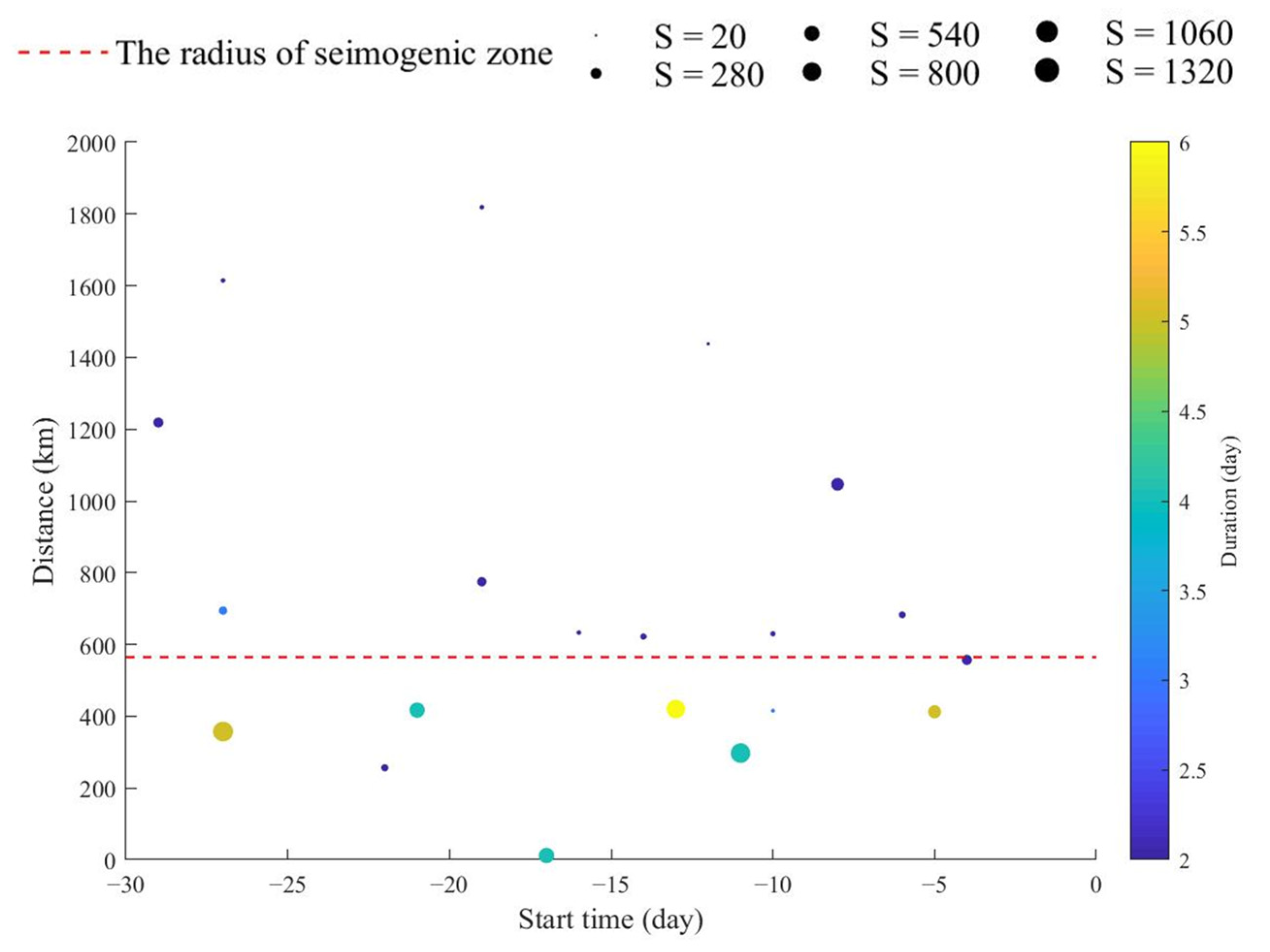
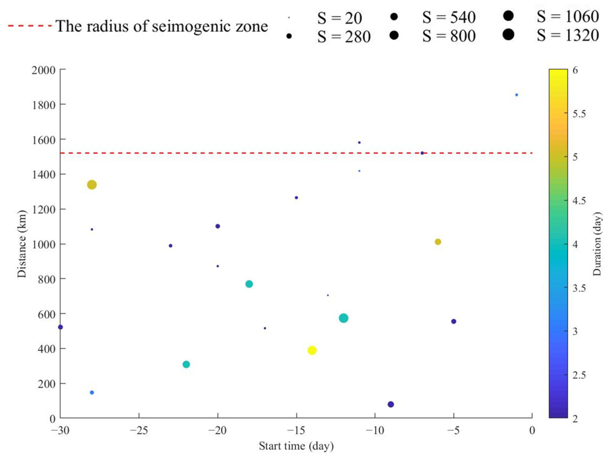
| Start Time (Day) | Duration (Day) | Distance 1 (km) | Distance 2 (km) | Coverage Area (Pixel) |
|---|---|---|---|---|
| −29 | 2 | 1218.514 | 522.3128 | 335 |
| −27 | 2 | 1614.612 | 1082.72 | 76 |
| −27 | 3 | 694.1449 | 147.2815 | 233 |
| −27 | 5 | 357.3739 | 1338.696 | 1310 |
| −22 | 2 | 256.0721 | 989.042 | 174 |
| −21 | 4 | 416.9308 | 308.354 | 777 |
| −19 | 2 | 1818.656 | 871.9 | 65 |
| −19 | 2 | 774.8023 | 1100.769 | 295 |
| −17 | 4 | 11.84356 | 769.3796 | 809 |
| −16 | 2 | 633.2236 | 515.8192 | 73 |
| −14 | 2 | 622.0482 | 1264.55 | 138 |
| −13 | 6 | 420.0436 | 388.9196 | 1157 |
| −12 | 2 | 1438.045 | 704.7843 | 40 |
| −11 | 4 | 297.1712 | 573.796 | 1261 |
| −10 | 3 | 415.1837 | 1417.791 | 48 |
| −10 | 2 | 629.9462 | 1580.574 | 85 |
| −8 | 2 | 1046.354 | 79.24198 | 545 |
| −6 | 2 | 682.544 | 1520.562 | 160 |
| −5 | 5 | 412.239 | 1011.247 | 562 |
| −4 | 2 | 557.2012 | 554.8826 | 349 |
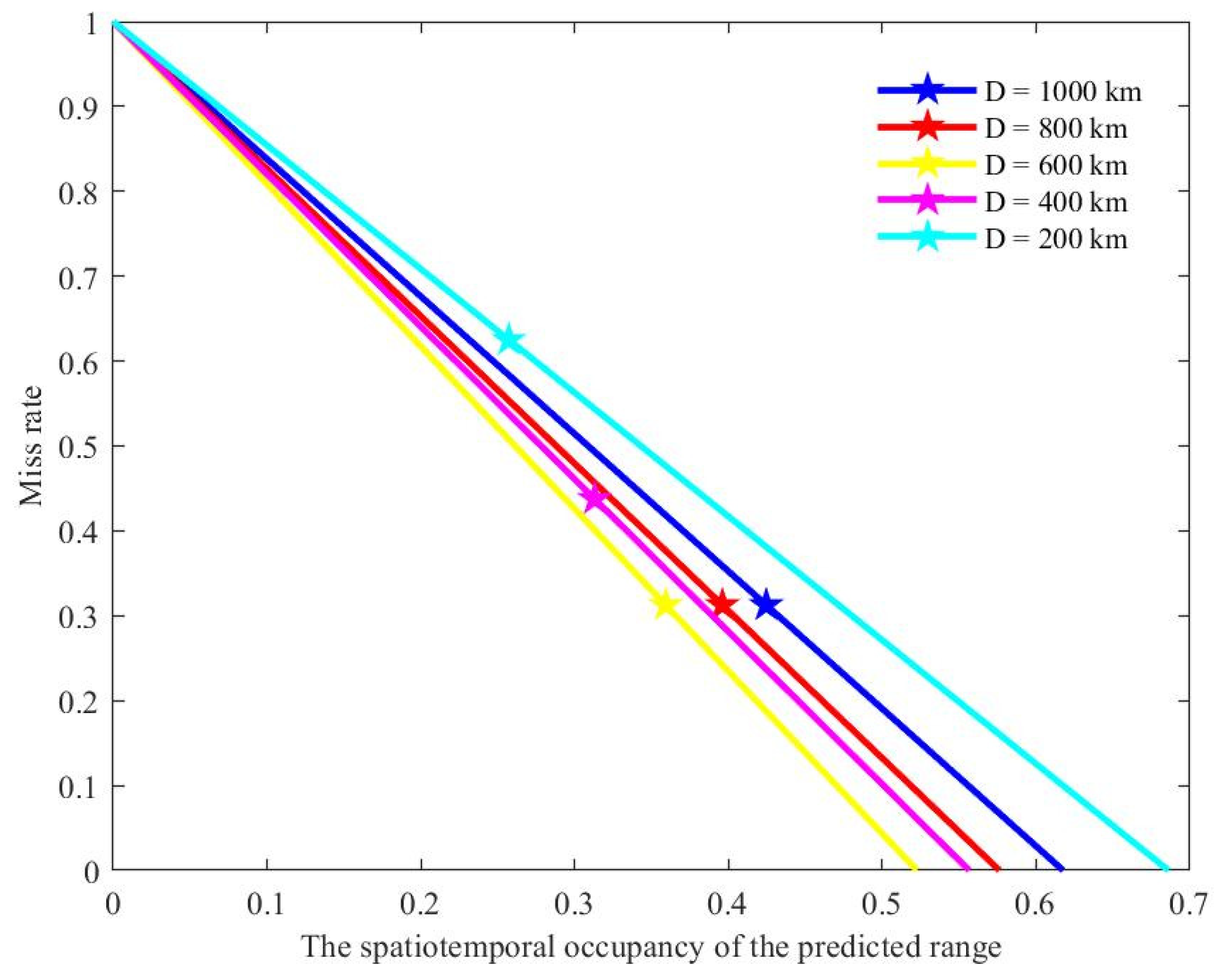
| Predicted Radius (km) | Correlation Rate | Hit Rate | Probability Gain |
|---|---|---|---|
| 1000 | 0.6429 | 0.6875 | 1.6193 |
| 800 | 0.6429 | 0.6875 | 1.7358 |
| 600 | 0.6429 | 0.6875 | 1.9137 |
| 400 | 0.5714 | 0.5625 | 1.7971 |
| 200 | 0.3571 | 0.375 | 1.4576 |
| Time (UTC+8) | Magnitude | Latitude (°N) | Longitude (°E) | Depth (km) |
|---|---|---|---|---|
| 16 September 2021, 04:33:31 | 6 | 29.2 | 105.34 | 10 |
| 26 August 2021, 07:38:18 | 5.5 | 38.88 | 95.5 | 15 |
| 13 August 2021, 12:21:35 | 5.8 | 34.58 | 97.54 | 8 |
| 29 July 2021, 16:39:27 | 5.7 | 22.7 | 96.04 | 20 |
| 7 July 2021, 14:43:48 | 5.2 | 19.65 | 101.2 | 10 |
| 16 June 2021, 16:48:58 | 5.8 | 38.14 | 93.81 | 10 |
| 12 June 2021, 18:00:46 | 5 | 24.96 | 97.89 | 16 |
| 10 June 2021, 19:46:07 | 5.1 | 24.34 | 101.91 | 8 |
| 22 May 2021, 02:04:11 | 7.4 | 34.59 | 98.34 | 17 |
| 21 May 2021, 21:48:34 | 6.4 | 25.67 | 99.87 | 8 |
| 19 March 2021, 14:11:26 | 6.1 | 31.94 | 92.74 | 10 |
Disclaimer/Publisher’s Note: The statements, opinions and data contained in all publications are solely those of the individual author(s) and contributor(s) and not of MDPI and/or the editor(s). MDPI and/or the editor(s) disclaim responsibility for any injury to people or property resulting from any ideas, methods, instructions or products referred to in the content. |
© 2023 by the authors. Licensee MDPI, Basel, Switzerland. This article is an open access article distributed under the terms and conditions of the Creative Commons Attribution (CC BY) license (https://creativecommons.org/licenses/by/4.0/).
Share and Cite
Yue, Y.; Chen, F.; Chen, G. Pre-Seismic Anomaly Detection from Multichannel Infrared Images of FY-4A Satellite. Remote Sens. 2023, 15, 259. https://doi.org/10.3390/rs15010259
Yue Y, Chen F, Chen G. Pre-Seismic Anomaly Detection from Multichannel Infrared Images of FY-4A Satellite. Remote Sensing. 2023; 15(1):259. https://doi.org/10.3390/rs15010259
Chicago/Turabian StyleYue, Yingbo, Fuchun Chen, and Guilin Chen. 2023. "Pre-Seismic Anomaly Detection from Multichannel Infrared Images of FY-4A Satellite" Remote Sensing 15, no. 1: 259. https://doi.org/10.3390/rs15010259