
Seasonal Variations of the Relationship between Spectral Indexes and Land Surface Temperature Based on Local Climate Zones: A Study in Three Yangtze River Megacities
 , ,
, ,  , , and
Abstract
:1. Introduction
2. Materials and Methods
2.1. Study Area
2.2. Data Collection
2.3. Methods
2.3.1. Spectral Indexes
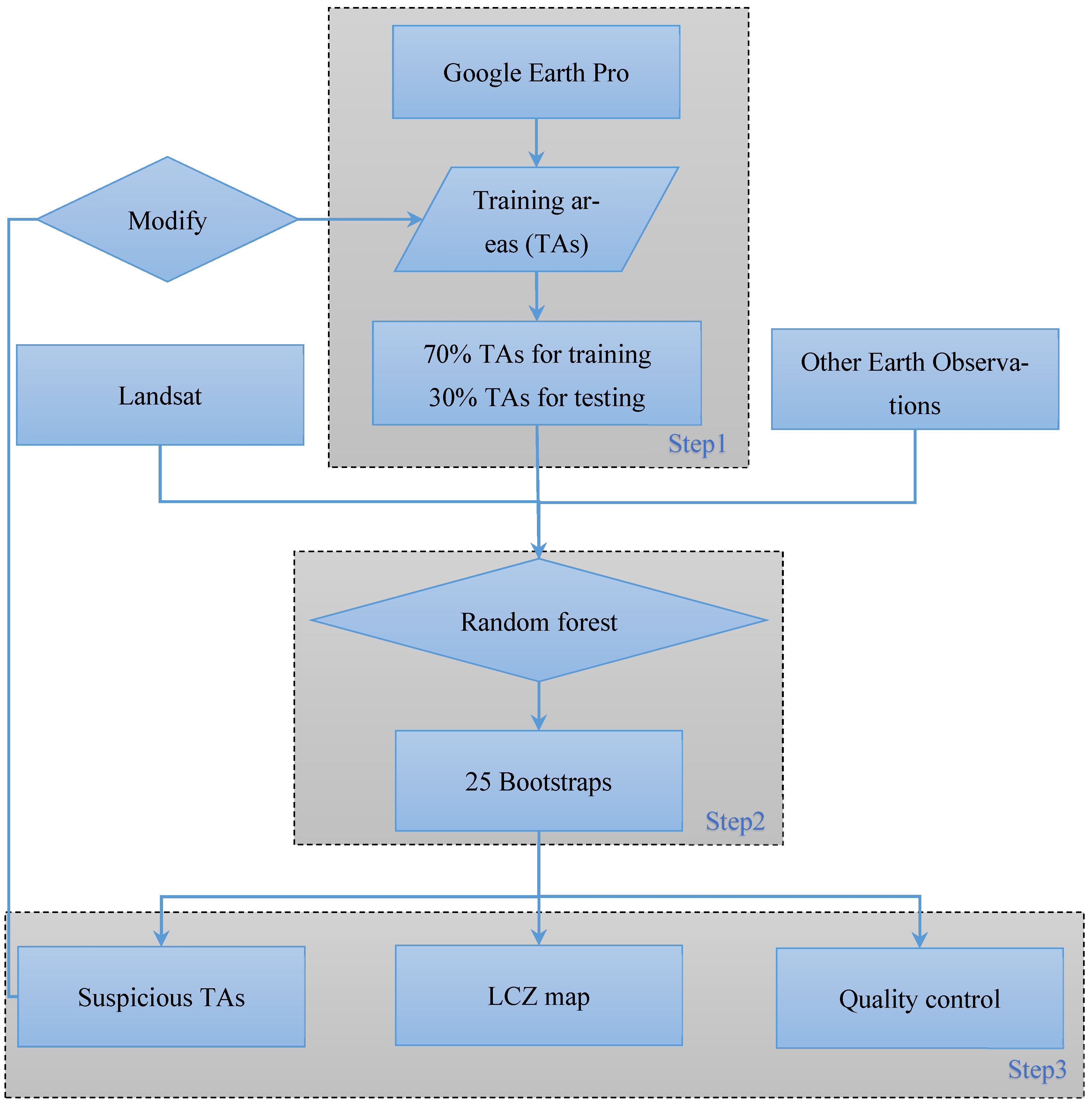
2.3.2. Classification of Local Climate Zones
2.3.3. Contribution of High-Temperature Zone
2.3.4. Analysis of Surface Urban Heat Islands Intensity
2.3.5. Analysis of Variance and Post Hoc Test
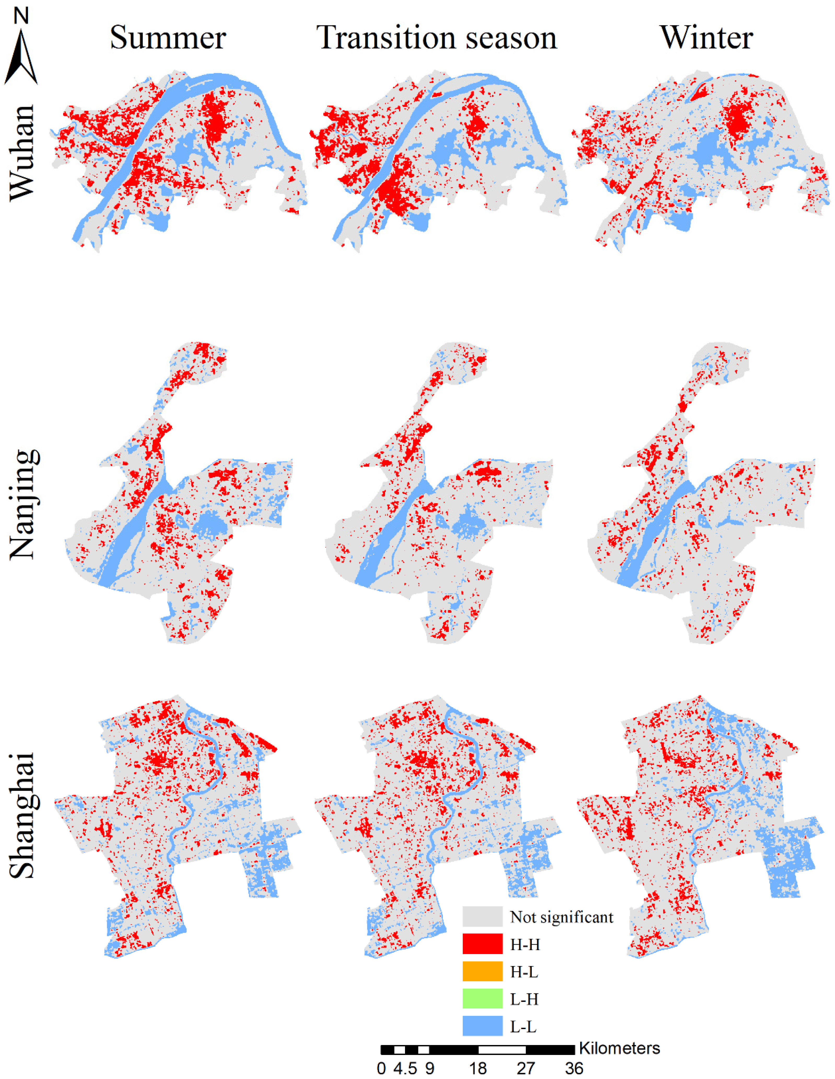
2.3.6. Spatial Pattern Characteristics of Land Surface Temperature
2.3.7. Geographically Weighted Regression
3. Results
3.1. Statistical Characteristics of Spectral Indexes and LST
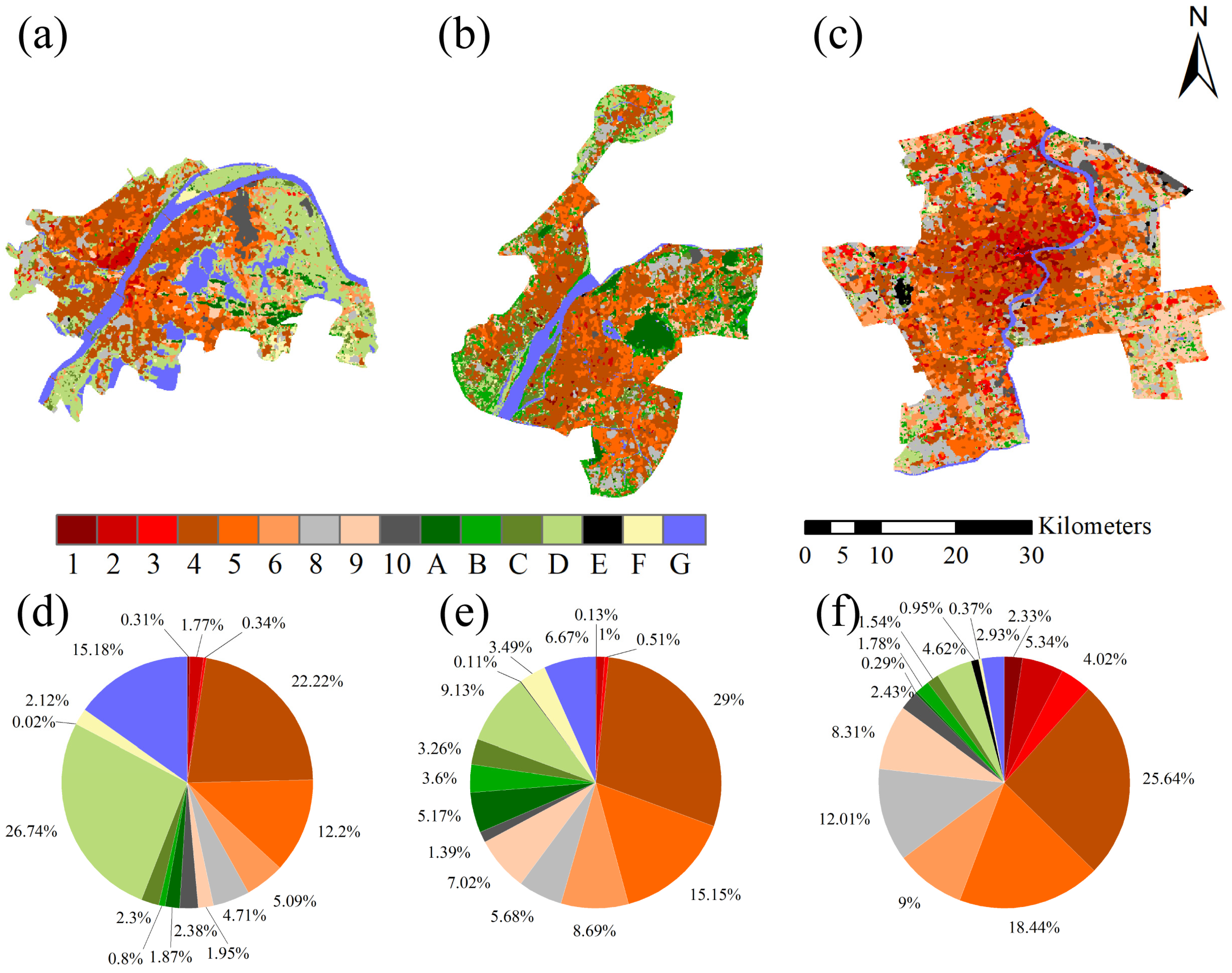
3.2. Classification of Local Climate Zones
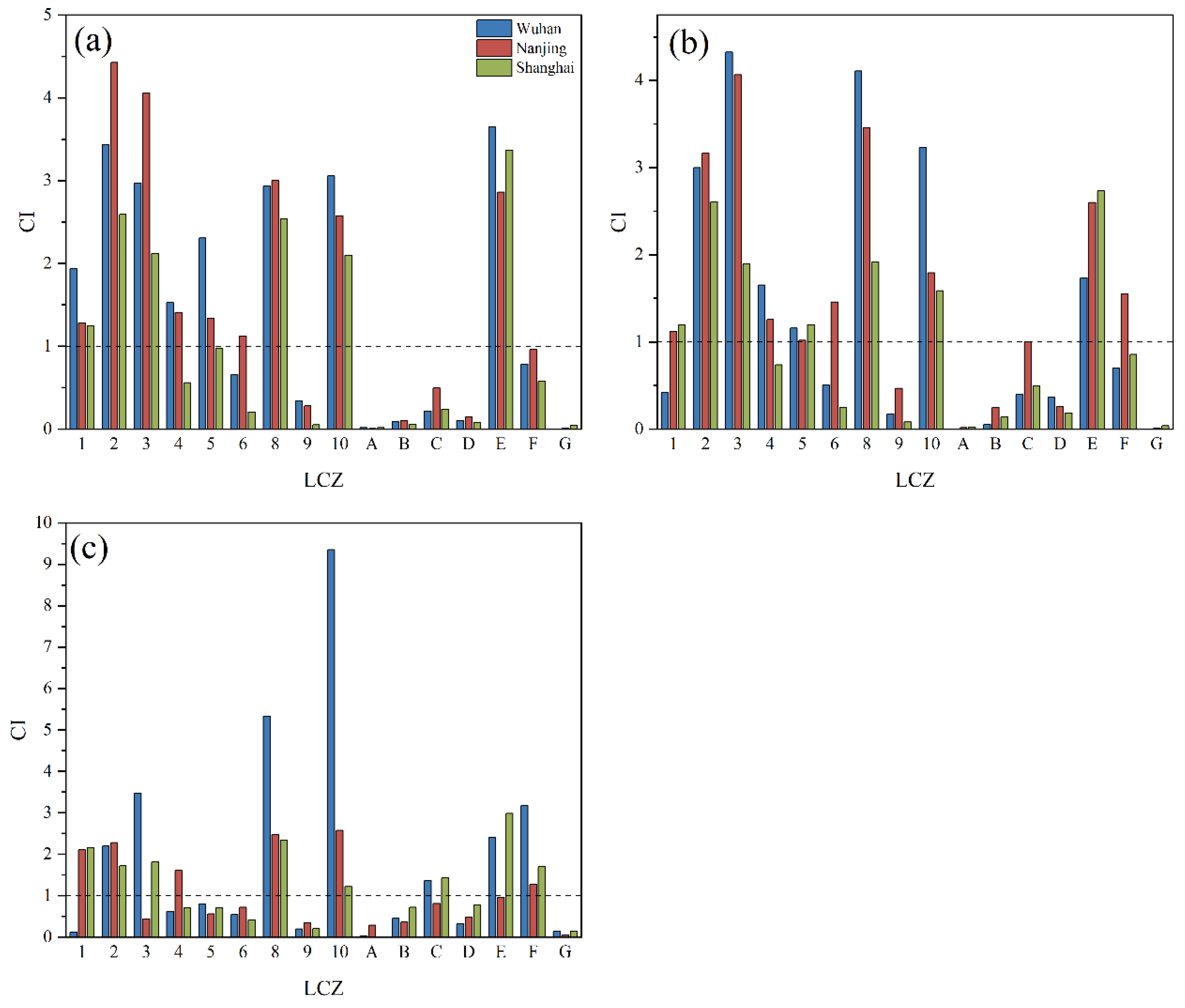
3.3. Contribution of Local Climatic Zones to High-Temperature Zones
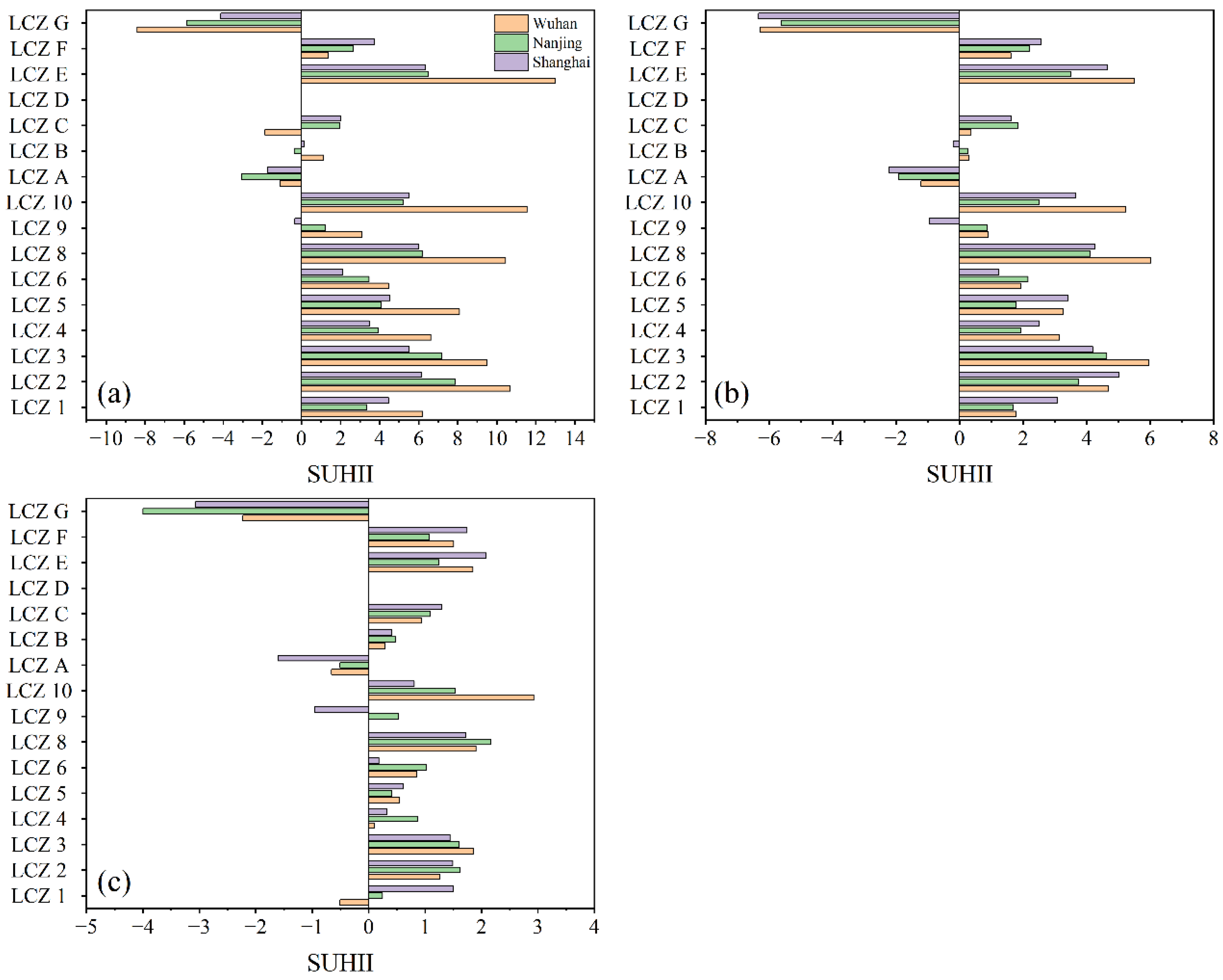
3.4. Surface Urban Heat Island Intensity
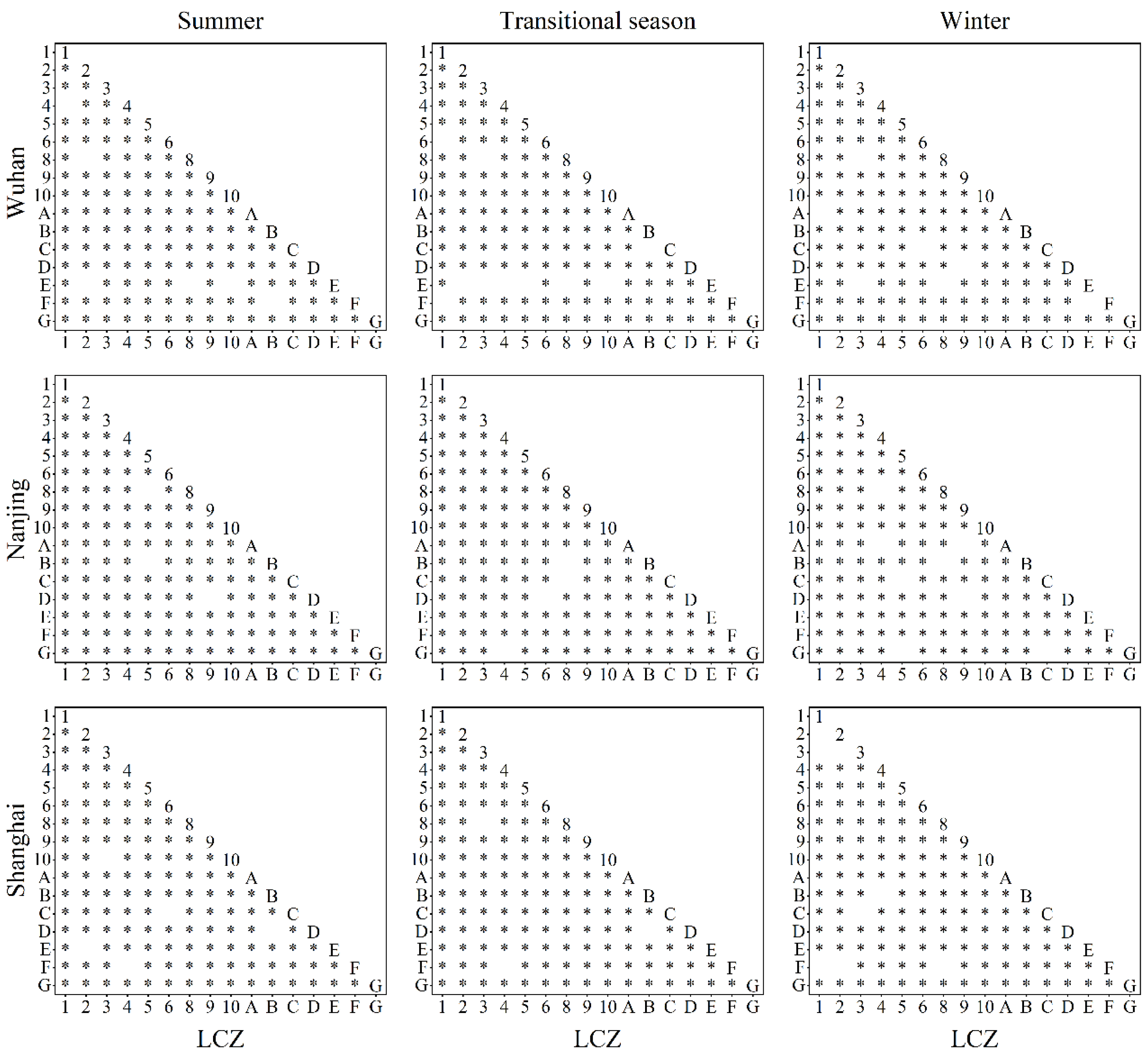
3.5. Analysis of Variance and Post Hoc Comparisons
3.6. Spatial Pattern Characteristics of Land Surface Temperature
3.7. The Relationship between Spectral Indexes and LST
4. Discussion
4.1. Thermal Contribution of LCZ and the Effect of SUHII
4.2. Policy Implications of Spectral Indexes in LCZs
4.3. Limitations
5. Conclusions
Author Contributions
Funding
Data Availability Statement
Acknowledgments
Conflicts of Interest
Appendix A


| City | Season | Date | Cloud Cover | Path/Row |
|---|---|---|---|---|
| Wuhan | Summer | 3 August 2020 | 1.98 | 123/39 |
| Transition seasons | 13 April 2020 29 April 2020 22 October 2020 | 3.11 | ||
| 2.70 | ||||
| 3.82 | ||||
| Winter | 25 December 2020 | 0.80 | ||
| Nanjing | Summer | 11 July 2019 12 August 2019 1 August 2021 | 18.65 | 120/38 |
| 12.18 | ||||
| 12.86 | ||||
| Transition seasons | 8 April 2020 24 April 2020 1 October 2020 18 November 2020 | 16.82 | ||
| 5.05 | ||||
| 3.39 | ||||
| 2.69 | ||||
| Winter | 20 December 2020 6 February 2021 22 February 2021 | 0.52 | ||
| 12.59 | ||||
| 19.10 | ||||
| Shanghai | Summer | 16 August 2020 | 2.17 | 118/38 |
| Transition season | 12 May 2020 | 15.85 | ||
| Winter | 22 December 2020 24 February 2021 | 0.61 | ||
| 13.84 |
| City | Season | Local Climate Zone | |||||||||||||||
|---|---|---|---|---|---|---|---|---|---|---|---|---|---|---|---|---|---|
| 1 | 2 | 3 | 4 | 5 | 6 | 8 | 9 | 10 | A | B | C | D | E | F | G | ||
| Wuhan | Summer | * | |||||||||||||||
| Transition season | |||||||||||||||||
| Winter | * | ||||||||||||||||
| Nanjing | Summer | * | |||||||||||||||
| Transition season | * | ||||||||||||||||
| Winter | |||||||||||||||||
| Shanghai | Summer | ||||||||||||||||
| Transition season | |||||||||||||||||
| Winter | |||||||||||||||||
| City | Season | F Statistic | df1 | df2 | Significance |
|---|---|---|---|---|---|
| Wuhan | Summer | 1120.058 | 15 | 95,447 | 0.000 |
| Transition season | 415.135 | 15 | 95,447 | 0.000 | |
| Winter | 1080.428 | 15 | 95,447 | 0.000 | |
| Nanjing | Summer | 114.394 | 15 | 90,073 | 0.000 |
| Transition season | 166.490 | 15 | 90,073 | 0.000 | |
| Winter | 276.668 | 15 | 90,073 | 0.000 | |
| Shanghai | Summer | 414.295 | 15 | 114,552 | 0.000 |
| Transition season | 493.091 | 15 | 114,552 | 0.000 | |
| Winter | 142.276 | 15 | 114,552 | 0.000 |
References
- Li, X.; Stringer, L.C.; Dallimer, M. The Role of Blue Green Infrastructure in the Urban Thermal Environment across Seasons and Local Climate Zones in East Africa. Sustain. Cities Soc. 2022, 80, 103798. [Google Scholar] [CrossRef]
- United Nations. World Urbanization Prospects: The 2018 Revision; The United Nations’ Department of Economic and Social Affairs—Population Division: New York, NY, USA, 2019; p. 126. [Google Scholar]
- Luo, J.; Wei, Y.H.D. Modeling Spatial Variations of Urban Growth Patterns in Chinese Cities: The Case of Nanjing. Landsc. Urban Plan. 2009, 91, 51–64. [Google Scholar] [CrossRef]
- Wang, Z.H. Reconceptualizing Urban Heat Island: Beyond the Urban-Rural Dichotomy. Sustain. Cities Soc. 2022, 77, 103581. [Google Scholar] [CrossRef]
- Wang, Z.H. Compound Environmental Impact of Urban Mitigation Strategies: Co-Benefits, Trade-Offs, and Unintended Consequence. Sustain. Cities Soc. 2021, 75, 103284. [Google Scholar] [CrossRef]
- Oke, T.R. City size and the urban heat island. Atmos. Environ. 1973, 7, 769–779. [Google Scholar] [CrossRef]
- Santamouris, M. On the Energy Impact of Urban Heat Island and Global Warming on Buildings. Energy Build. 2014, 82, 100–113. [Google Scholar] [CrossRef]
- Ngarambe, J.; Joen, S.J.; Han, C.H.; Yun, G.Y. Exploring the Relationship between Particulate Matter, CO, SO2, NO2, O3 and Urban Heat Island in Seoul, Korea. J. Hazard. Mater. 2021, 403, 123615. [Google Scholar] [CrossRef]
- Heaviside, C.; Macintyre, H.; Vardoulakis, S. The Urban Heat Island: Implications for Health in a Changing Environment. Curr. Environ. Health Rep. 2017, 4, 296–305. [Google Scholar] [CrossRef]
- Youngsteadt, E.; Ernst, A.F.; Dunn, R.R.; Frank, S.D. Responses of Arthropod Populations to Warming Depend on Latitude: Evidence from Urban Heat Islands. Glob. Chang. Biol. 2017, 23, 1436–1447. [Google Scholar] [CrossRef]
- Santamouris, M.; Cartalis, C.; Synnefa, A. Local Urban Warming, Possible Impacts and a Resilience Plan to Climate Change for the Historical Center of Athens, Greece. Sustain. Cities Soc. 2015, 19, 281–291. [Google Scholar] [CrossRef]
- Xiang, Y.; Huang, C.; Huang, X.; Zhou, Z.; Wang, X. Seasonal Variations of the Dominant Factors for Spatial Heterogeneity and Time Inconsistency of Land Surface Temperature in an Urban Agglomeration of Central China. Sustain. Cities Soc. 2021, 75, 103285. [Google Scholar] [CrossRef]
- Zhou, D.; Xiao, J.; Bonafoni, S.; Berger, C.; Deilami, K.; Zhou, Y.; Frolking, S.; Yao, R.; Qiao, Z.; Sobrino, J.A. Satellite Remote Sensing of Surface Urban Heat Islands: Progress, Challenges, and Perspectives. Remote Sens. 2019, 11, 48. [Google Scholar] [CrossRef]
- Anniballe, R.; Bonafoni, S.; Pichierri, M. Spatial and Temporal Trends of the Surface and Air Heat Island over Milan Using MODIS Data. Remote Sens. Environ. 2014, 150, 163–171. [Google Scholar] [CrossRef]
- Deilami, K.; Kamruzzaman, M.; Liu, Y. Urban Heat Island Effect: A Systematic Review of Spatio-Temporal Factors, Data, Methods, and Mitigation Measures. Int. J. Appl. Earth Obs. Geoinf. 2018, 67, 30–42. [Google Scholar] [CrossRef]
- Mathew, A.; Khandelwal, S.; Kaul, N. Analysis of Diurnal Surface Temperature Variations for the Assessment of Surface Urban Heat Island Effect over Indian Cities. Energy Build. 2018, 159, 271–295. [Google Scholar] [CrossRef]
- Singh, V.K.; Bhati, S.; Mohan, M.; Sahoo, N.R.; Dash, S. Numerical Simulation of the Impact of Urban Canopies and Anthropogenic Emissions on Heat Island Effect in an Industrial Area: A Case Study of Angul-Talcher Region in India. Atmos. Res. 2022, 277, 106320. [Google Scholar] [CrossRef]
- Xiang, Y.; Ye, Y.; Peng, C.; Teng, M.; Zhou, Z. Seasonal Variations for Combined Effects of Landscape Metrics on Land Surface Temperature (LST) and Aerosol Optical Depth (AOD). Ecol. Indic. 2022, 138, 108810. [Google Scholar] [CrossRef]
- Peng, J.; Jia, J.; Liu, Y.; Li, H.; Wu, J. Seasonal Contrast of the Dominant Factors for Spatial Distribution of Land Surface Temperature in Urban Areas. Remote Sens. Environ. 2018, 215, 255–267. [Google Scholar] [CrossRef]
- Xie, Q.; Wu, Y.; Zhou, Z.; Wang, Z. Remote Sensing Study of the Impact of Vegetation on Thermal Environment in Different Contexts. IOP Conf. Ser. Earth Environ. Sci. 2018, 121, 22009. [Google Scholar] [CrossRef]
- Liu, S.; Wu, Y.; Xu, J.; Zhang, L. Relationship between surface thermal environment and underlying surface index in Yan’an city. J. Northwest A&F Univ. 2022, 37, 207214. [Google Scholar] [CrossRef]
- Jenerette, G.D.; Harlan, S.L.; Buyantuev, A.; Stefanov, W.L.; Declet-Barreto, J.; Ruddell, B.L.; Myint, S.W.; Kaplan, S.; Li, X. Micro-Scale Urban Surface Temperatures Are Related to Land-Cover Features and Residential Heat Related Health Impacts in Phoenix, AZ USA. Landsc. Ecol. 2016, 31, 745–760. [Google Scholar] [CrossRef]
- Yu, Z.; Xu, S.; Zhang, Y.; Jørgensen, G.; Vejre, H. Strong Contributions of Local Background Climate to the Cooling Effect of Urban Green Vegetation. Sci. Rep. 2018, 8, 6798. [Google Scholar] [CrossRef] [PubMed]
- Chen, W.; Zhang, J.; Shi, X.; Liu, S. Impacts of Building Features on the Cooling Effect of Vegetation in Community-Based Microclimate: Recognition, Measurement and Simulation from a Case Study of Beijing. Int. J. Environ. Res. Public Health 2020, 17, 8915. [Google Scholar] [CrossRef] [PubMed]
- Yang, G.; Yu, Z.; Jørgensen, G.; Vejre, H. How Can Urban Blue-Green Space Be Planned for Climate Adaption in High-Latitude Cities? A Seasonal Perspective. Sustain. Cities Soc. 2020, 53, 101932. [Google Scholar] [CrossRef]
- Guerri, G.; Crisci, A.; Messeri, A.; Congedo, L.; Munafò, M.; Morabito, M. Thermal Summer Diurnal Hot-Spot Analysis: The Role of Local Urban Features Layers. Remote Sens. 2021, 13, 538. [Google Scholar] [CrossRef]
- Fan, H.; Yu, Z.; Yang, G.; Liu, T.Y.; Liu, T.Y.; Hung, C.H.; Vejre, H. How to Cool Hot-Humid (Asian) Cities with Urban Trees? An Optimal Landscape Size Perspective. Agric. For. Meteorol. 2019, 265, 338–348. [Google Scholar] [CrossRef]
- Bechtel, B.; Alexander, P.J.; Böhner, J.; Ching, J.; Conrad, O.; Feddema, J.; Mills, G.; See, L.; Stewart, I. Mapping Local Climate Zones for a Worldwide Database of the Form and Function of Cities. ISPRS Int. J. Geo-Inf. 2015, 4, 199–219. [Google Scholar] [CrossRef]
- Aslam, A.; Rana, I.A. The Use of Local Climate Zones in the Urban Environment: A Systematic Review of Data Sources, Methods, and Themes. Urban Clim. 2022, 42, 101120. [Google Scholar] [CrossRef]
- Stewart, I.D.; Oke, T.R. Local Climate Zones for Urban Temperature Studies. Bull. Am. Meteorol. Soc. 2012, 93, 1879–1900. [Google Scholar] [CrossRef]
- Lyu, T.; Buccolieri, R.; Gao, Z. A Numerical Study on the Correlation between Sky View Factor and Summer Microclimate of Local Climate Zones. Atmosphere 2019, 10, 438. [Google Scholar] [CrossRef] [Green Version]
- Yang, J.; Ren, J.; Sun, D.; Xiao, X.; Xia, J.C.; Jin, C.; Li, X. Understanding Land Surface Temperature Impact Factors Based on Local Climate Zones. Sustain. Cities Soc. 2021, 69, 102818. [Google Scholar] [CrossRef]
- Sun, F.; Zhao, H.; Deng, L.; Liu, Y.; Cheng, R.; Che, Y. Characterizing the Warming Effect of Increasing Temperatures on Land Surface: Temperature Change, Heat Pattern Dynamics and Thermal Sensitivity. Sustain. Cities Soc. 2021, 70, 102904. [Google Scholar] [CrossRef]
- Wang, L.; Hou, H.; Weng, J. Ordinary Least Squares Modelling of Urban Heat Island Intensity Based on Landscape Composition and Configuration: A Comparative Study among Three Megacities along the Yangtze River. Sustain. Cities Soc. 2020, 62, 102381. [Google Scholar] [CrossRef]
- Li, K.; Chen, Y.; Wang, M.; Gong, A. Spatial-Temporal Variations of Surface Urban Heat Island Intensity Induced by Different Definitions of Rural Extents in China. Sci. Total Environ. 2019, 669, 229–247. [Google Scholar] [CrossRef] [PubMed]
- Geng, S.; Yang, L.; Sun, Z.; Wang, Z.; Qian, J.; Jiang, C.; Wen, M. Spatiotemporal Patterns and Driving Forces of Remotely Sensed Urban Agglomeration Heat Islands in South China. Sci. Total Environ. 2021, 800, 149499. [Google Scholar] [CrossRef]
- Demuzere, M.; Kittner, J.; Bechtel, B. LCZ Generator: A Web Application to Create Local Climate Zone Maps. Front. Environ. Sci. 2021, 9, 637455. [Google Scholar] [CrossRef]
- Peng, J.; Xie, P.; Liu, Y.; Ma, J. Urban Thermal Environment Dynamics and Associated Landscape Pattern Factors: A Case Study in the Beijing Metropolitan Region. Remote Sens. Environ. 2016, 173, 145–155. [Google Scholar] [CrossRef]
- Ke, X.; Men, H.; Zhou, T.; Li, Z.; Zhu, F. Variance of the Impact of Urban Green Space on the Urban Heat Island Effect among Different Urban Functional Zones: A Case Study in Wuhan. Urban For. Urban Green. 2021, 62, 127159. [Google Scholar] [CrossRef]
- Hu, D.; Meng, Q.; Schlink, U.; Hertel, D.; Liu, W.; Zhao, M.; Guo, F. How Do Urban Morphological Blocks Shape Spatial Patterns of Land Surface Temperature over Different Seasons? A Multifactorial Driving Analysis of Beijing, China. Int. J. Appl. Earth Obs. Geoinf. 2022, 106, 102648. [Google Scholar] [CrossRef]
- Bechtel, B.; Demuzere, M.; Mills, G.; Zhan, W.; Sismanidis, P.; Small, C.; Voogt, J. SUHI Analysis Using Local Climate Zones—A Comparison of 50 Cities. Urban Clim. 2019, 28, 100451. [Google Scholar] [CrossRef]
- Unal Cilek, M.; Cilek, A. Analyses of Land Surface Temperature (LST) Variability among Local Climate Zones (LCZs) Comparing Landsat-8 and ENVI-Met Model Data. Sustain. Cities Soc. 2021, 69, 102877. [Google Scholar] [CrossRef]
- Badaro-Saliba, N.; Adjizian-Gerard, J.; Zaarour, R.; Najjar, G. LCZ Scheme for Assessing Urban Heat Island Intensity in a Complex Urban Area (Beirut, Lebanon). Urban Clim. 2021, 37, 100846. [Google Scholar] [CrossRef]
- Guo, A.; Yang, J.; Sun, W.; Xiao, X.; Xia Cecilia, J.; Jin, C.; Li, X. Impact of Urban Morphology and Landscape Characteristics on Spatiotemporal Heterogeneity of Land Surface Temperature. Sustain. Cities Soc. 2020, 63, 102443. [Google Scholar] [CrossRef]
- Mouzourides, P.; Eleftheriou, A.; Kyprianou, A.; Ching, J.; Neophytou, M.K.A. Linking Local-Climate-Zones Mapping to Multi-Resolution-Analysis to Deduce Associative Relations at Intra-Urban Scales through an Example of Metropolitan London. Urban Clim. 2019, 30, 100505. [Google Scholar] [CrossRef]
- La, Y.; Bagan, H.; Yamagata, Y. Urban Land Cover Mapping under the Local Climate Zone Scheme Using Sentinel-2 and PALSAR-2 Data. Urban Clim. 2020, 33, 100661. [Google Scholar] [CrossRef]
- Wan, J.Z. Pasture Availability as a Spatial Indicator of Grassland Root Turnover Time on a Global Scale. Ecol. Indic. 2020, 111, 105985. [Google Scholar] [CrossRef]
- Yang, M.; Gao, X.; Zhao, X.; Wu, P. Scale Effect and Spatially Explicit Drivers of Interactions between Ecosystem Services—A Case Study from the Loess Plateau. Sci. Total Environ. 2021, 785, 147389. [Google Scholar] [CrossRef]
- Yu, Z.; Yang, G.; Zuo, S.; Jørgensen, G.; Koga, M.; Vejre, H. Critical Review on the Cooling Effect of Urban Blue-Green Space: A Threshold-Size Perspective. Urban For. Urban Green. 2020, 49, 126630. [Google Scholar] [CrossRef]
- Shuai, C.; Sha, J.; Lin, J.; Ji, W.; Zhou, Z.; Gao, S. Spatial difference of the relationship between remote sensing index and land surface temperature under different underlying surfaces. Geo-Inf. Sci. 2018, 20, 1657–1666. [Google Scholar] [CrossRef]
- Roy, S.; Pandit, S.; Eva, E.A.; Bagmar, M.S.H.; Papia, M.; Banik, L.; Dube, T.; Rahman, F.; Razi, M.A. Examining the Nexus between Land Surface Temperature and Urban Growth in Chattogram Metropolitan Area of Bangladesh Using Long Term Landsat Series Data. Urban Clim. 2020, 32, 100593. [Google Scholar] [CrossRef]
- Hathway, E.A.; Sharples, S. The Interaction of Rivers and Urban Form in Mitigating the Urban Heat Island Effect: A UK Case Study. Build. Environ. 2012, 58, 14–22. [Google Scholar] [CrossRef]
- Geletič, J.; Lehnert, M.; Savić, S.; Milošević, D. Inter-/Intra-Zonal Seasonal Variability of the Surface Urban Heat Island Based on Local Climate Zones in Three Central European Cities. Build. Environ. 2019, 156, 21–32. [Google Scholar] [CrossRef]
- Eldesoky, A.H.M.; Gil, J.; Pont, M.B. The Suitability of the Urban Local Climate Zone Classification Scheme for Surface Temperature Studies in Distinct Macroclimate Regions. Urban Clim. 2021, 37, 100823. [Google Scholar] [CrossRef]


| Built Types | Land Cover Types | ||
|---|---|---|---|
| Class | Description | Class | Description |
| LCZ 1 | Compact high-rise | LCZ A | Dense trees |
| LCZ 2 | Compact mid-rise | LCZ B | Scattered trees |
| LCZ 3 | Compact low-rise | LCZ C | Bush, scrub |
| LCZ 4 | Open high-rise | LCZ D | Low plants |
| LCZ 5 | Open mid-rise | LCZ E | Bare rock or paved |
| LCZ 6 | Open low-rise | LCZ F | Bare soil or sand |
| LCZ 8 | Large low-rise | LCZ G | Water |
| LCZ 9 | Sparsely built | ||
| LCZ 10 | Heavy industry | ||
| City | Season | LST (°C) | MNDWI | NDBI | NDVI |
|---|---|---|---|---|---|
| Wuhan | Summer | 44.00 ± 7.02 | −0.14 ± 0.45 | −0.18 ± 0.19 | 0.28 ± 0.41 |
| Transition season | 27.57 ± 4.25 | −0.10 ± 0.34 | −0.16 ± 0.13 | 0.25 ± 0.29 | |
| Winter | 11.65 ± 1.89 | 0.001 ± 0.31 | −0.11 ± 0.14 | 0.12 ± 0.21 | |
| Nanjing | Summer | 39.20 ± 4.16 | −0.25 ± 0.25 | −0.18 ± 0.13 | 0.42 ± 0.25 |
| Transition season | 27.93 ± 2.84 | −0.20 ± 0.24 | −0.14 ± 0.11 | 0.33 ± 0.22 | |
| Winter | 15.63 ± 2.40 | −0.19 ± 0.26 | −0.05 ± 0.11 | 0.21 ± 0.20 | |
| Shanghai | Summer | 45.25 ± 3.46 | −0.26 ± 0.19 | −0.14 ± 0.13 | 0.38 ± 0.24 |
| Transition season | 37.15 ± 3.28 | −0.25 ± 0.16 | −0.12 ± 0.13 | 0.34 ± 0.22 | |
| Winter | 15.75 ± 2.22 | −0.17 ± 0.17 | −0.07 ± 0.10 | 0.22 ± 0.16 |
| City | Season | Statistic | df1 | df2 | Significance |
|---|---|---|---|---|---|
| Wuhan | Summer | 19,310.390 | 15 | 1028.742 | 0.000 |
| Transition season | 19,288.741 | 15 | 1028.556 | 0.000 | |
| Winter | 2747.871 | 15 | 1030.775 | 0.000 | |
| Nanjing | Summer | 8016.538 | 15 | 1741.385 | 0.000 |
| Transition season | 6199.907 | 15 | 1741.496 | 0.000 | |
| Winter | 3365.614 | 15 | 1743.017 | 0.000 | |
| Shanghai | Summer | 5808.144 | 15 | 9367.378 | 0.000 |
| Transition season | 4903.839 | 15 | 9364.059 | 0.000 | |
| Winter | 1425.392 | 15 | 9378.346 | 0.000 |
| City | Season | Moran’s Index | z-Score | p-Value |
|---|---|---|---|---|
| Wuhan | Summer | 0.95 | 574.47 | <0.001 |
| Transition season | 0.93 | 564.06 | <0.001 | |
| Winter | 0.86 | 520.92 | <0.001 | |
| Nanjing | Summer | 0.92 | 386.88 | <0.001 |
| Transition season | 0.91 | 383.73 | <0.001 | |
| Winter | 0.75 | 317.32 | <0.001 | |
| Shanghai | Summer | 0.87 | 416.87 | <0.001 |
| Transition season | 0.87 | 415.65 | <0.001 | |
| Winter | 0.82 | 389.50 | <0.001 |
| City | Season | MNDWI | NDVI | NDBI |
|---|---|---|---|---|
| Wuhan | Summer | 0.83 | 0.88 | 0.89 |
| Transition season | 0.83 | 0.85 | 0.86 | |
| Winter | 0.75 | 0.75 | 0.78 | |
| Nanjing | Summer | 0.74 | 0.67 | 0.83 |
| Transition season | 0.78 | 0.78 | 0.82 | |
| Winter | 0.57 | 0.56 | 0.54 | |
| Shanghai | Summer | 0.84 | 0.86 | 0.89 |
| Transition season | 0.87 | 0.87 | 0.88 | |
| Winter | 0.79 | 0.80 | 0.81 |
| Indices | LCZ | Wuhan | Nanjing | Shanghai | ||||||
|---|---|---|---|---|---|---|---|---|---|---|
| Summ | Tran | Wint | Summ | Tran | Wint | Summ | Tran | Wint | ||
| MNDWI | 1 | −8.98 | −7.78 | −4.03 | −0.12 | −4.57 | −3.88 | −1.53 | −3.25 | −3.97 |
| 2 | −11.81 | −9.47 | −4.05 | 0.23 | −2.97 | −1.56 | 0.88 | −0.22 | −2.14 | |
| 3 | −7.95 | −7.16 | −4.34 | −5.78 | −6.11 | −5.10 | 1.56 | −0.95 | −1.57 | |
| 4 | −5.29 | −6.71 | −4.90 | 1.33 | −3.01 | −2.65 | 3.20 | 1.68 | −2.25 | |
| 5 | −3.97 | −5.68 | −4.37 | 3.22 | −1.77 | −2.52 | 2.57 | 1.23 | −1.14 | |
| 6 | −2.85 | −4.82 | −4.04 | 7.13 | 1.14 | −1.41 | 5.33 | 2.51 | −0.44 | |
| 8 | −4.32 | −5.88 | −4.85 | 5.14 | 0.68 | −1.72 | 2.86 | 0.55 | −0.98 | |
| 9 | −3.25 | −4.82 | −4.29 | 10.10 | 2.70 | −0.72 | 4.98 | 2.30 | −0.42 | |
| 10 | 2.42 | 2.48 | 0.63 | 3.63 | −2.60 | −2.34 | 1.21 | −0.85 | −1.56 | |
| A | 1.95 | −1.85 | −4.05 | 10.85 | 0.30 | −3.48 | 7.34 | 4.73 | −0.17 | |
| B | −1.18 | −3.99 | −3.95 | 5.50 | −0.08 | −1.92 | 5.38 | 2.22 | −1.21 | |
| C | −6.25 | −6.35 | −3.45 | 3.14 | −1.78 | −2.42 | 5.50 | 2.11 | −1.55 | |
| D | −4.96 | −6.14 | −4.27 | 1.07 | −2.17 | −3.47 | 4.37 | −0.56 | −1.90 | |
| E | 1.12 | −2.73 | −6.33 | −2.97 | −3.44 | −3.89 | 5.99 | 1.84 | −1.15 | |
| F | 0.00 | −4.39 | −4.57 | 2.94 | −1.81 | -2.13 | 2.67 | −0.26 | −1.26 | |
| G | −9.49 | −8.12 | −3.52 | −6.47 | −6.44 | −3.56 | −7.43 | −9.85 | −5.12 | |
| NDVI | 1 | 3.04 | 2.69 | 4.65 | −1.43 | 0.63 | 0.86 | −0.87 | 0.33 | 0.92 |
| 2 | 2.85 | 1.89 | 4.26 | −5.17 | −1.75 | 0.33 | −3.30 | −2.45 | −1.70 | |
| 3 | −1.47 | −2.24 | 1.83 | −0.84 | 0.74 | 3.23 | −4.83 | −2.98 | −0.90 | |
| 4 | −1.15 | 0.35 | 4.85 | −4.08 | −0.83 | 0.33 | −4.26 | −3.03 | −1.54 | |
| 5 | −2.99 | −1.52 | 2.47 | −5.75 | −1.90 | 0.36 | −3.77 | −2.71 | −1.36 | |
| 6 | −3.41 | −1.59 | 1.93 | −9.07 | −4.23 | −0.40 | −5.13 | −3.28 | −1.25 | |
| 8 | −4.86 | −3.54 | 2.74 | −8.26 | −4.71 | −0.63 | −4.36 | −2.22 | −0.82 | |
| 9 | −2.86 | −0.45 | 2.15 | −9.84 | −4.52 | −0.87 | −5.33 | −3.55 | −1.17 | |
| 10 | −6.51 | −7.15 | −4.23 | −5.31 | −0.94 | 0.23 | −2.03 | −0.12 | 0.37 | |
| A | −5.15 | −2.29 | 0.68 | −11.90 | −3.48 | 1.73 | −6.49 | −4.79 | −1.63 | |
| B | −2.42 | −0.42 | 1.63 | −6.82 | −2.22 | 0.84 | −5.02 | −2.91 | −0.51 | |
| C | −0.16 | 0.06 | 0.33 | −0.12 | −0.51 | 1.48 | −0.20 | 0.07 | −0.21 | |
| D | 0.62 | 2.10 | 3.88 | −4.38 | −0.36 | 2.94 | −4.59 | −1.69 | −0.07 | |
| E | −13.55 | −7.40 | −4.19 | −1.47 | 0.97 | 4.94 | −4.53 | −1.48 | 0.78 | |
| F | −1.92 | 2.17 | 5.09 | −4.90 | −0.63 | 1.25 | −4.13 | −1.27 | 0.28 | |
| G | 7.92 | 8.25 | 4.18 | 5.79 | 6.93 | 4.69 | 8.50 | 12.22 | 7.11 | |
| NDBI | 1 | 15.09 | 13.37 | 6.76 | 11.76 | 9.05 | 7.74 | 7.25 | 6.26 | 6.57 |
| 2 | 17.18 | 13.78 | 7.02 | 12.52 | 6.62 | 3.28 | 6.74 | 5.83 | 5.14 | |
| 3 | 18.17 | 12.69 | 6.33 | 17.45 | 13.04 | 7.66 | 9.84 | 7.74 | 4.36 | |
| 4 | 14.73 | 11.98 | 6.15 | 13.43 | 8.87 | 6.50 | 7.72 | 6.13 | 5.68 | |
| 5 | 13.97 | 10.43 | 6.04 | 13.74 | 8.64 | 5.15 | 6.76 | 5.32 | 3.58 | |
| 6 | 17.63 | 12.69 | 5.91 | 14.93 | 8.91 | 3.36 | 8.58 | 5.96 | 3.29 | |
| 8 | 19.78 | 13.56 | 6.87 | 15.51 | 10.19 | 4.37 | 9.51 | 6.52 | 4.20 | |
| 9 | 14.35 | 11.30 | 5.66 | 15.90 | 9.02 | 3.36 | 9.57 | 6.89 | 3.60 | |
| 10 | 18.09 | 13.58 | 4.22 | 14.08 | 8.48 | 5.20 | 8.07 | 5.85 | 3.45 | |
| A | 14.31 | 11.25 | 5.23 | 19.15 | 8.84 | 3.08 | 11.47 | 8.25 | 4.27 | |
| B | 15.65 | 11.95 | 4.95 | 16.39 | 10.26 | 4.41 | 9.85 | 6.68 | 4.13 | |
| C | 18.77 | 16.41 | 5.39 | 14.49 | 10.55 | 5.41 | 9.47 | 7.07 | 3.68 | |
| D | 14.81 | 14.35 | 6.72 | 15.78 | 11.30 | 5.40 | 9.14 | 5.61 | 3.92 | |
| E | 26.43 | 11.88 | 8.81 | 21.13 | 15.22 | 8.02 | 8.74 | 3.74 | 2.13 | |
| F | 13.06 | 17.40 | 6.81 | 14.73 | 10.14 | 5.05 | 8.07 | 5.49 | 2.84 | |
| G | 8.71 | 17.90 | 5.04 | 16.72 | 16.92 | 8.56 | 15.58 | 20.26 | 10.74 | |
Disclaimer/Publisher’s Note: The statements, opinions and data contained in all publications are solely those of the individual author(s) and contributor(s) and not of MDPI and/or the editor(s). MDPI and/or the editor(s) disclaim responsibility for any injury to people or property resulting from any ideas, methods, instructions or products referred to in the content. |
© 2023 by the authors. Licensee MDPI, Basel, Switzerland. This article is an open access article distributed under the terms and conditions of the Creative Commons Attribution (CC BY) license (https://creativecommons.org/licenses/by/4.0/).
Share and Cite
Xiang, Y.; Tang, Y.; Wang, Z.; Peng, C.; Huang, C.; Dian, Y.; Teng, M.; Zhou, Z. Seasonal Variations of the Relationship between Spectral Indexes and Land Surface Temperature Based on Local Climate Zones: A Study in Three Yangtze River Megacities. Remote Sens. 2023, 15, 870. https://doi.org/10.3390/rs15040870
Xiang Y, Tang Y, Wang Z, Peng C, Huang C, Dian Y, Teng M, Zhou Z. Seasonal Variations of the Relationship between Spectral Indexes and Land Surface Temperature Based on Local Climate Zones: A Study in Three Yangtze River Megacities. Remote Sensing. 2023; 15(4):870. https://doi.org/10.3390/rs15040870
Chicago/Turabian StyleXiang, Yang, Yongqi Tang, Zhihua Wang, Chucai Peng, Chunbo Huang, Yuanyong Dian, Mingjun Teng, and Zhixiang Zhou. 2023. "Seasonal Variations of the Relationship between Spectral Indexes and Land Surface Temperature Based on Local Climate Zones: A Study in Three Yangtze River Megacities" Remote Sensing 15, no. 4: 870. https://doi.org/10.3390/rs15040870