Fast Resolution Enhancement for Real Beam Mapping Using the Parallel Iterative Deconvolution Method

Abstract

Super-resolution methods for real beam mapping (RBM) imagery play a significant role in many microwave remote sensing applications. However, the existing super-resolution methods require high-dimensional matrix operations in the case of wide-field imaging, which makes it difficult to satisfy the requirements of real-time signal processing. To solve this problem, this paper introduces an improved Poisson distribution-based maximum likelihood (IPML) method by adding an adaptive iterative acceleration factor to effectively improve the algorithm convergence speed without introducing high-dimensional matrix operations. Furthermore, a GPU-based parallel processing architecture is proposed through the multithreading characteristics of the computing platform, and a cooperative CPU–GPU working model is constructed. This can realize the parallel optimization of the echo reception, preprocessing, and super-resolution processing. We verify that the proposed parallel super-resolution method can significantly improve the computational efficiency without sacrificing performance, using a real dataset.

1. Introduction

Real beam mapping (RBM) has attracted attention for various modern remote sensing applications, such as surface surveillance, path navigation, weather monitoring, and target strikes as it has a dense revisit time and allows for wide-area observations under an arbitrary geometry [1,2,3,4]. The RBM system achieves high resolution in the range dimension through matched filtering, but its azimuth resolution is still limited by the antenna aperture [5,6,7].

More recently, super-resolution technology has been used to break through the limitations of the angular resolution and has been extensively studied. Super-resolution technology extracts effective information from low-resolution blurred images and reconstructs image details, enabling image reconstruction and separating adjacent targets within the mainlobe [8,9]. At present, super-resolution imaging methods can be divided into three main categories, including inverse filtering methods [10,11,12], regularization methods [13,14], and spectral estimation methods [15,16]. In [17,18], a classical inverse filtering method called Wiener filtering was proposed to achieve super-resolution imaging, but it had a smoothing effect due to its low-pass filtering properties, and its angular resolution enhancement was unsatisfactory. In [2,14,19], the total variation (TV) and the $L_1$ and $L_2$ norms were introduced as constrained terms in the regularization framework; then, the essence of the super-resolution imaging was transformed into a convex optimization problem. In addition, an iterative reweighted least square (IRLS) method based on truncated singular value decomposition (TSVD) was proposed for super-resolution imaging [20,21,22]. This suppressed noise by cutting some small singular value components in the antenna pattern measurement matrix, which caused information loss due to the truncation operation. However, the resolution improvement in the above super-resolution methods requires numerous matrix inversions and multiplication operations, which reduces the computational efficiency. Spectral estimation approaches, such as an extended multiple signal classification (MUSIC) algorithm and a capon beamforming method, were put forward in [23,24]. However, the improvement in resolution caused by these methods required the accumulation of a large number of snapshots. In [25], the authors proposed an iterative adaptive approach (IAA) to achieve RBM super-resolution imaging, which utilized one snapshot to realize a higher azimuth resolution. Regrettably, the improvements in the angular resolution obtained by the existing regularization methods and the spectral estimation methods came at the cost of an extremely high computational complexity, including high-dimensional matrix multiplication and inversion, which reduce the imaging efficiency and use a large amount of storage space resources [26,27,28].

Recently, various Bayesian methods have been proposed in RBM super-resolution imaging [29,30]. In these methods, reasonable prior assumptions of noise and targets can be introduced based on a maximum a posteriori (MAP) criterion [31,32,33], which can obtain a higher angular resolution in different applications. However, during actual RBM signal processing, the noise distribution is unknown; therefore, the above methods have limited improvements in resolution. In addition, the regularization operator, sparse norm terms, and other optimization terms were considered prior information in these super-resolution algorithms, and obtained better resolution enhancement in RBM super-resolution imaging [34,35,36]. Unfortunately, the Bayesian methods required multiple iterative operations, and the convergence speed was slow and could not meet the real-time imaging required in practical applications.

To enable real-time super-resolution imaging, an improved Poisson distribution maximum likelihood method is introduced in this paper, which effectively improves the iterative processing of the algorithm by introducing an adaptive iterative acceleration factor. In addition, this paper proposes a parallel optimization processing architecture based on a GPU, which was used to accelerate the processing of the range pulse compression and the super-resolution. Compared with the CPU serial processing method, the GPU parallel processing method can greatly improve computational efficiency.

The rest of the paper is organized as follows. In Section 2, the echo model of the RBM is introduced. In Section 3, the improved Poisson distribution-based maximum likelihood method (IPML) is introduced in detail. In Section 4, the effectiveness of the introduced algorithm is verified by the simulation and real data-processing results. Section 5 introduces the parallel processing architecture of the super-resolution imaging algorithm using the GPU platform and uses the experiment data to verify the superiority of the parallel processing method. Our conclusions are discussed in Section 6.

2. Echo Model

This section introduces the continuous and discrete signal model in the RBM working mode; we mainly consider the one-dimensional echo signal model with a stationary platform.

2.1. Continuous Signal Model

In RBM imaging mode, the antenna beam scans the entire imaging area, while a pulse radar transmits a typical chirp signal at a certain pulse repetition frequency to improve the range resolution. To obtain a two-dimensional microwave image with the radar position as the center of the circle, the circular beam scans in the azimuth direction at a certain scanning speed while transmitting the pulse signal. During the interval between adjacent transmission pulses, the received echo signals can be expressed as [37,38]:

$$\begin{array}{c}\hfill \begin{array}{c}y\left(\theta \right)={\int }_{\mathsf{\Phi }}s\left(\theta \right)h\left(\theta \right)d\theta \end{array},\end{array}$$

(1)

where $y\left(\theta \right)$ denotes the received RBM echo signal, $s\left(\theta \right)$ is the target scattering coefficient, $h\left(\theta \right)$ is the antenna function, and $\mathsf{\Phi }$ denotes the antenna beam scanning range.

2.2. Discrete Signal Model

In RBM imaging, the microwave sensor transmits a linear frequency modulated (LFM) signal with a large bandwidth [39]. After range pulse compression, we can obtain a high resolution in the range dimension. In order to make the resolution in the azimuth and range dimension consistent, we focus on the improvements in resolution in the azimuth dimension. The azimuth signal model of the RBM system can be expressed as follows:

$$\begin{array}{c}\hfill \begin{array}{c}\mathbf{y}=\mathbf{h}\otimes \mathbf{s}+\mathbf{n}\end{array},\end{array}$$

(2)

where $\mathbf{y}\in {\mathbb{C}}^{M\times 1}$, $\mathbf{h}\in {\mathbb{C}}^{L\times 1}$, $\mathbf{s}\in {\mathbb{C}}^{K\times 1}$, and $\mathbf{n}\in {\mathbb{C}}^{M\times 1}$ denote the vectors of the azimuth echo, the antenna pattern, the reflectivity function, and the noise term, respectively. The symbol ⊗ represents the convolution operation, and K and L denote the lengths of the antenna pattern and the reflectivity function vectors, respectively, which are defined by

$$\begin{array}{c}\hfill \begin{array}{c}L={\displaystyle \frac{\Delta \theta }{\Omega }}PRF\end{array},\end{array}$$

(3)

$$\begin{array}{c}\hfill \begin{array}{c}M=K+L-1\end{array},\end{array}$$

(4)

where M represents the number of azimuth echo sampling points, $\Omega$ represents the antenna scanning speed, and $\Delta \theta$ is the coverage area scanned by the antenna. Therefore, the reconstruction of $\mathbf{s}$ from the measurements $\mathbf{y}$ in the time domain becomes a classical deconvolution problem. Rewriting (2) in matrix form, we have:

$$\begin{array}{c}\hfill \begin{array}{c}\mathbf{y}=\mathbf{As}+\mathbf{n}\end{array},\end{array}$$

(5)

where:

$$\begin{array}{c}\hfill \begin{array}{c}\mathbf{A}=\left[\begin{array}{cccc}{h}_1& & & \\ h_2& h_1& & \\ ⋮& h_2& \ddots & \\ h_L& ⋮& \ddots & h_1\\ & h_L& & h_2\\ & & \ddots & ⋮\\ & & & h_L\end{array}\right]\triangleq \left[{\mathbf{a}}_1,{\mathbf{a}}_2,\dots ,{\mathbf{a}}_K\right]\end{array}.\end{array}$$

(6)

3. Improved Poisson Distribution-Based Maximum Likelihood Super-Resolution Imaging Algorithm

3.1. Poisson Distribution-Based Maximum Likelihood Super-Resolution Imaging Algorithm

The essential problem of the RBM azimuth super-resolution algorithm is how to solve the deconvolution problem. Direct deconvolution is inherently ill-conditioned. In this section, an iterative deconvolution method based on the maximum likelihood criterion is introduced in detail [29]. The resulting algorithm can transform the pathological nature of the direct deconvolution into benignity and restore the high-frequency scattering information of the target.

We assume that the $mth$ element in the azimuth echo signal is independent and satisfies the Poisson distribution and the influence of the noise is ignored [30]; that is,

$$\begin{array}{c}\hfill \begin{array}{c}{\mathbf{y}}_m=poisson\left({\left(\mathbf{As}\right)}_m\right)\end{array}.\end{array}$$

(7)

Using the properties of the Poisson distribution, the expectation and variance of each element of the azimuth echo signal can be expressed as follows:

$$\begin{array}{c}\hfill \begin{array}{c}D\left({\mathbf{y}}_m\right)={\widehat{\mathbf{y}}}_m={\displaystyle \sum _{k=0}^{K-1}}{\mathbf{A}}_{mk}{\mathbf{s}}_k\end{array},\end{array}$$

(8)

where the variance and expectation are denoted by $D\left({\mathbf{y}}_m\right)$ and ${\widehat{\mathbf{y}}}_m$.

The probability distribution of the likelihood function of each element of the azimuth echo signal is:

$$\begin{array}{c}\hfill \begin{array}{c}p({\mathbf{y}}_m/\mathbf{s})={\displaystyle \frac{{\left({\displaystyle \sum _{k=0}^{K-1}}{\mathbf{A}}_{mk}{\mathbf{s}}_k\right)}^{{\mathbf{y}}_m}}{{\mathbf{y}}_m!}}{e}^{-{\displaystyle \sum _{k=0}^{K-1}}{\mathbf{A}}_{mk}{\mathbf{s}}_k}\end{array}.\end{array}$$

(9)

Since the elements of the azimuth echo signal vector are independent from each other, the joint distribution probability likelihood function of each element of the echo signal $\mathbf{s}$ is:

$$\begin{array}{c}\hfill \begin{array}{c}p(\mathbf{y}/\mathbf{s})={\displaystyle \prod _{m=0}^{M-1}}{\displaystyle \frac{{\left({\displaystyle \sum _{k=0}^{K-1}}{\mathbf{A}}_{mk}{\mathbf{s}}_k\right)}^{{\mathbf{y}}_m}}{{\mathbf{y}}_m!}}{e}^{-{\displaystyle \sum _{k=0}^{K-1}}{\mathbf{A}}_{mk}{\mathbf{s}}_k}\end{array}.\end{array}$$

(10)

According to the Bayesian criterion [32,33],

$$\begin{array}{c}\hfill \begin{array}{c}p(\mathbf{s}/\mathbf{y})={\displaystyle \frac{p(\mathbf{y}/\mathbf{s})p\left(\mathbf{s}\right)}{p\left(\mathbf{y}\right)}}\end{array},\end{array}$$

(11)

where $p(\mathbf{s}/\mathbf{y})$ is the probability distribution of the target under the condition of a known echo signal probability distribution, $p(\mathbf{y}/\mathbf{s})$ is the joint probability distribution likelihood function of each element of the echo signal, and $p\left(\mathbf{s}\right)$ the target probability distribution.

In actual RBM imaging, since $p\left(\mathbf{s}\right)$ cannot be known in real time, it can be assumed that it is subject to a uniform distribution; then, the maximum likelihood estimate is:

$$\begin{array}{c}\hfill \begin{array}{c}\widehat{f}=arg\underset{f}{max}p(\mathbf{y}/\mathbf{s})\end{array}.\end{array}$$

(12)

It can be seen from (11) that when the likelihood function $p(\mathbf{y}/\mathbf{s})$ is the largest, the estimated value that is obtained $p(\mathbf{s}/\mathbf{y})$ can more closely represent the azimuth scattering information of the target. To obtain the maximum value of $p(\mathbf{y}/\mathbf{s})$, logarithms are taken on both sides of (10):

$$\begin{array}{c}\hfill \begin{array}{c}lnp(\mathbf{y}/\mathbf{s})={\displaystyle \sum _{m=0}^{M-1}}\left({\mathbf{y}}_{m}ln{\displaystyle \sum _{k=0}^{K-1}}{\mathbf{A}}_{mk}{\mathbf{y}}_m-{\displaystyle \sum _{k=0}^{K-1}}{\mathbf{A}}_{mk}{\mathbf{s}}_k-ln{\mathbf{y}}_m!\right)\end{array}.\end{array}$$

(13)

When evaluating $p(\mathbf{y}/\mathbf{s})$, we can set the derivative of (13) as zero, resulting in:

$$\begin{array}{c}\hfill \begin{array}{c}{\displaystyle \sum _{m=0}^{M-1}}{\mathbf{A}}_{mk}({\displaystyle \frac{{\mathbf{y}}_m}{{\displaystyle \sum _{k=0}^{K-1}}{\mathbf{A}}_{mk}{\mathbf{s}}_k}}-1)=0\end{array}.\end{array}$$

(14)

In the practical processing of RBM imaging, it is necessary to perform normalization processing for $\mathbf{a}$; therefore, (14) can be transformed into:

$$\begin{array}{c}\hfill \begin{array}{c}{\mathbf{A}}^T\left({\displaystyle \frac{\mathbf{y}}{\mathbf{As}}}\right)=\mathbf{I}\end{array},\end{array}$$

(15)

where $\mathbf{I}$ is a unit vector.

Using the method of an iterative solution of an equation, the iterative solution of (15) can be obtained as:

$$\begin{array}{c}\hfill \begin{array}{c}{\mathbf{s}}^{i+1}={\mathbf{s}}^i\left[{\mathbf{A}}^T\left({\displaystyle \frac{\mathbf{y}}{\mathbf{A}{\mathbf{s}}^i}}\right)\right]\end{array},\end{array}$$

(16)

where ${\mathbf{s}}^i$ is the solution of the ith iterative iteration.

3.2. Adaptive Selection of Iteration Factor

There is a problem of convergence speed in the iterative solution. The iterative solution method of (16) can be improved by adding an iterative acceleration factor [40], which is

$$\begin{array}{c}\hfill \begin{array}{c}{\mathbf{s}}^{i+1}={\left[{\mathbf{A}}^T\left({\displaystyle \frac{\mathbf{y}}{\mathbf{A}{\mathbf{s}}^i}}\right)\right]}^q{\mathbf{s}}^i\end{array}.\end{array}$$

(17)

Compared with the iterative solution formulas of (16) and (17), when the iterative acceleration factor q of (17) is greater than 1, the iterative convergence acceleration can be achieved. However, the iterative process of (17) is only stable when the value range of the iterative acceleration factor q is between 1 and 3. Taking a larger value in this range can effectively speed up the iterative convergence process, but this increases the risk of solution instability at the same time; however, taking a smaller value slows down the iterative convergence speed, but can reduce the risk of solution instability [40,41].

In order to determine the optimal selection of the iterative acceleration factor q, an adaptive selection of the iterative acceleration factor q is given by the following expression:

$$\begin{array}{c}\hfill \begin{array}{c}q(k+1)=exp\left({\displaystyle \frac{{∥\nabla {\mathbf{s}}^i∥}_2}{{∥\nabla {\mathbf{s}}^{i-1}∥}_2}}\right)-{\displaystyle \frac{{∥\nabla {\mathbf{s}}^2∥}_2}{{∥\nabla {\mathbf{s}}^1∥}_2}}\end{array},\end{array}$$

(18)

where $\nabla {\mathbf{s}}^i$ is the first derivative of ${\mathbf{s}}^i$, and ${∥•∥}_2$ represents the $L_2$ norm of the vector. $\nabla {\mathbf{s}}^i$ characterizes the rate of change of the signal, which is the degree of azimuth sharpening from the perspective of the entire RBM echo signal. In the initial stage of iteration, the adaptive iteration acceleration factor represented by (18) will be greater than 3. At this time, the second term of (18) will limit the iteration acceleration factor to be much greater than 3, maintaining the stability of the iterative process. In the whole iterative process, at the initial stage, the convergence speed of the iterative process can be accelerated due to the exponential term of the iterative acceleration factor. The reason for this is that as the number of iterations increases, the iterative result gradually approaches the real value and the iterative acceleration factor gradually converges to 1, ensuring the stability of the iterative results. Therefore, the adaptive iteration acceleration factor is a good tradeoff and leads to a reconciliation between the iteration convergence speed and stability [42].

In order to initialize the accelerated iterative algorithm, the first two iterations of q must choose a fixed value ($1⩽q⩽3$). The value of q is generally selected as 1 to ensure stability at the initial stage of the iteration.

4. Simulation and Real Data Processing Results

In this section, we compare the super-resolution performance of the REGU method [14], the TSVD method [43], the TV method [19], the PML method, and the IPML method by conducting some simulations.

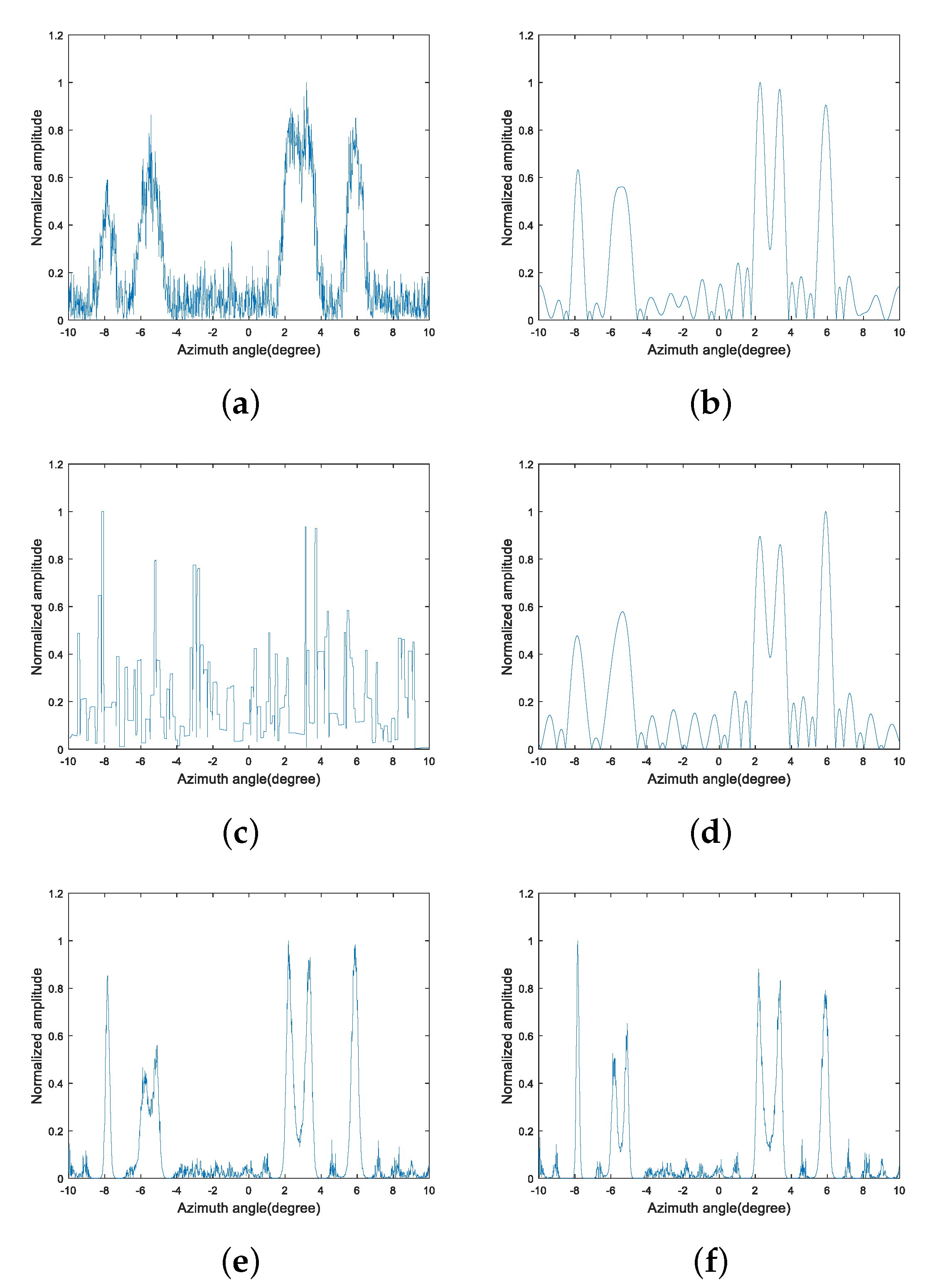
4.1. Point Target Simulation

This section compares the IPML method with other traditional super-resolution methods to verify its excellent imaging performance. The simulation parameters of the point simulation are shown in

Table 1. Simulation parameters.

Parameters	Value
Antenna beamwidth	1.2°
Antenna scanning speed	30°/s
Carrier frequency	30 GHz
Bandwidth	2 MHz
Pulse width	5 $\mathsf{\mu }$s
Pulse repetition frequency	1500 Hz
Scanning range	−10°–10°

. As shown in Figure 1a, the RBM antenna pattern, with its 3 dB beam width, was about 1.2 degrees. The point target distribution scene is shown in Figure 1b; the point target included two groups, and each group consisted of an isolated target and two relative neighboring targets. The width of the left target was 0.4 degrees, the width between adjacent targets was 0.3 degrees, and the target amplitude was 0.8; the width of the right target was 0.6 degrees, the width between adjacent targets was 0.4, and the target amplitude was 1.

In order to simulate in the same environment, we added different Gaussian white noise. Therefore, the signal-to-noise ratio (SNR) is defined as:

$$\begin{array}{c}\hfill \begin{array}{c}\mathrm{SNR}=10{log}_{10}{\displaystyle \frac{{∥\mathbf{s}∥}_2^2}{{∥\mathbf{y}-\mathbf{As}∥}_2^2}}.\end{array}\end{array}$$

(19)

First, we conducted simulations under a high SNR situation, and the processing results are shown in Figure 2. Figure 2a shows the raw RBM echo with Gaussian noise, with the SNR set to 30 dB. As the interval between the adjacent point targets is less than the beamwidth, the adjacent targets could not be distinguished. The result processed by the REGU method is shown in Figure 2b. The adjacent targets could be distinguished, but the target amplitude showed a certain loss. The processing result of the TV method is shown in Figure 2c. Compared with the REGU method, this had a higher resolution, but there were still some sidelobes affecting the resolution and the processing result was not smooth enough. Figure 2d shows the processing result of the TSVD method. A better azimuth resolution was achieved; since the cutoff value was an empirical selection parameter, it still had higher sidelobes. Figure 2e and Figure 2f represent the processing results of the PML method and IPML method, respectively. They had a visibly higher angular resolution and lower sidelobes than the other traditional methods.

To further demonstrate the effectiveness of the algorithm introduced in this paper, we conducted some simulations under a low SNR situation. We compared the processing results with the above methods, with SNR = 10 dB. The raw RBM echo with Gaussian noise is shown in Figure 3a. The processing result of the REGU method is shown in Figure 3b, the angular resolution became weaker, and the sidelobes were raised. The processing results of the TV method and the TSVD method are shown in Figure 3c and Figure 3d, respectively. There was a ladder effect and more false targets in the TV method, and the noise was amplified in the TSVD method. In contrast, the processing results of the PML method and the IPML method, shown in Figure 3e and Figure 3f, respectively, had a better angular resolution and noise-suppression ability. Furthermore, the super-resolution performance of the REGU method, the TV method, and the TSVD method were poorer in a higher noise environment, the sidelobe protrusions were more severe, and false targets were generated. The PML method and IPML method still had a good super-resolution performance, but sidelobes remained due to noise.

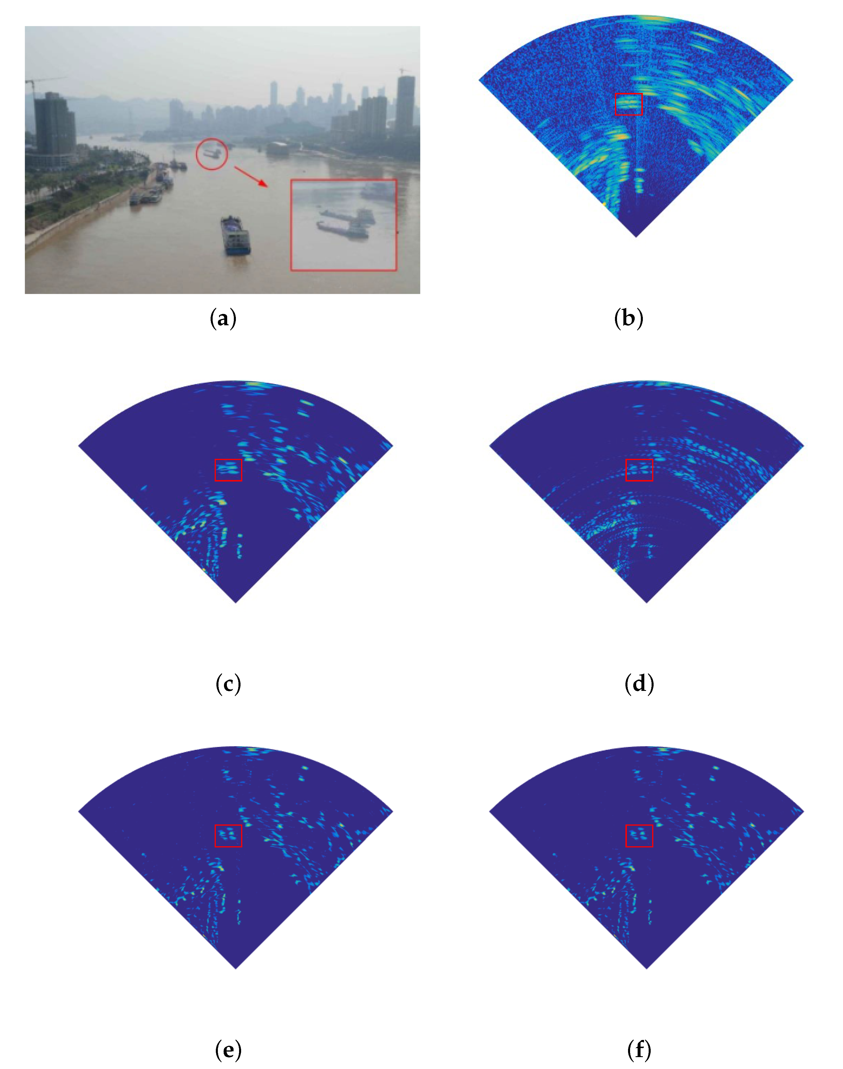
4.2. Real Data Processing

To verify the effectiveness of the IPML method in this section, we carried out verification experiments at Chaotianmen bridge, Chongqing, China. The RBM system parameters are shown in

Table 2. System Parameters.

Parameter	Value
Carrier frequency	X band
Beam width	5.1°
Bandwidth	75 MHz
PRF	204 Hz
Scanning speed	72°/s

. There are two groups of boats marked with the red circles on the Changjiang River, as shown by Figure 4a.

The real beam data are shown in Figure 4b. We cannot distinguish the two boats and the whole scene is drowned in noise. The processing results obtained by the REGU method are shown in Figure 4c; the two boats can barely separate, but the outline of the boats is almost distorted. The processing results obtained by the TSVD method are shown in Figure 4d; we can distinguish the distribution of the two boats. Regrettably, many parasitic ripples appear. The processing results obtained by the PML method and the IPML method are shown in Figure 4e,f. We can clearly distinguish the two boats and the IPML method can suppress the noise and clutter well.

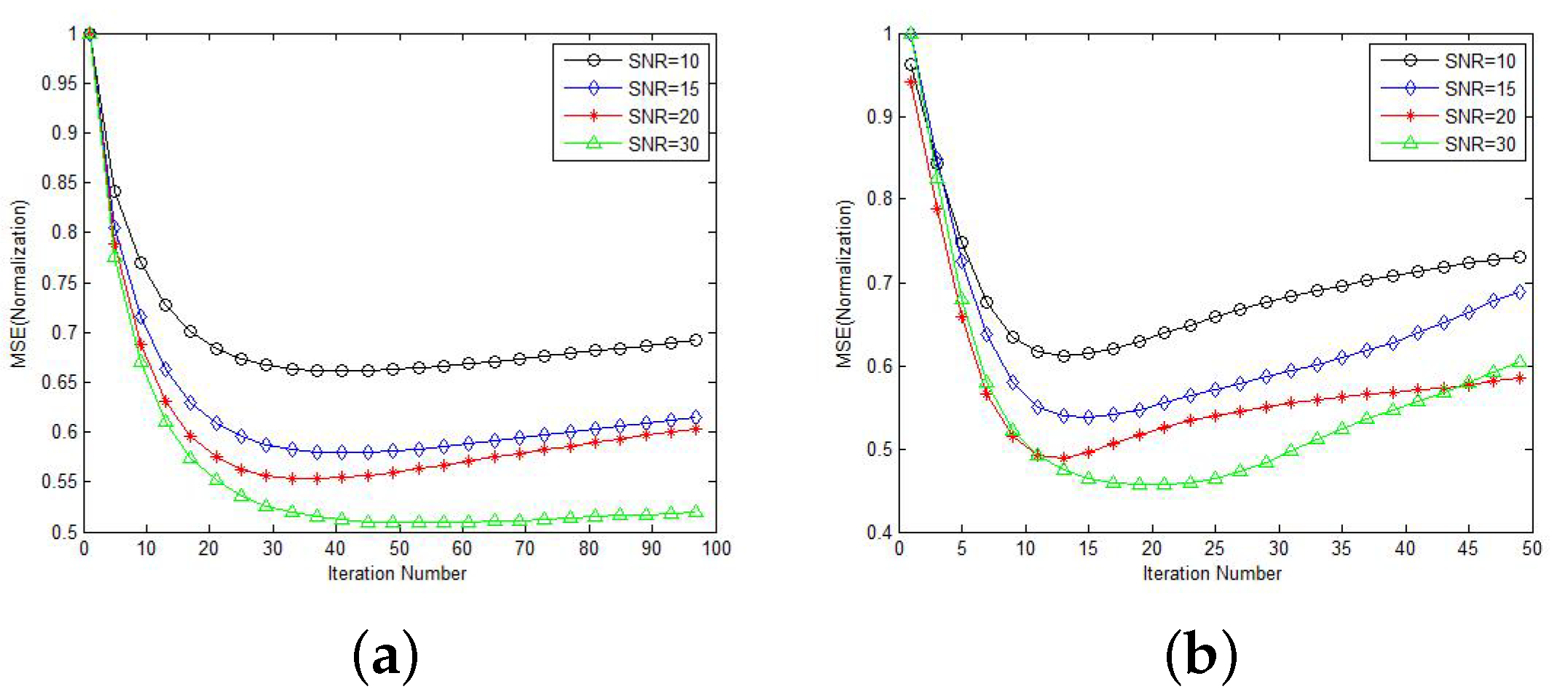
4.3. Error and Speedup Analysis

Under different signal-to-noise ratio conditions, the comparison of the convergence speed of the super-resolution algorithm with the accelerated iterative factor and the general iterative algorithm is shown through a plot of the mean square error in Figure 5. Through the comparison of the mean square error curve of the two iterative processes (the PML and the IPML), the Poisson distribution-based super-resolution algorithm (PML) generally needs to process more than 40 iterations to obtain the optimal iterative result, while the improved Poisson distribution-based super-resolution algorithm (IPML) can obtain the optimal result after about 15 iterations. Therefore, the improved super-resolution algorithm effectively increased the iterative convergence speed by more than two times, and the mean square error of the optimal point was smaller, which improved the super-resolution performance.

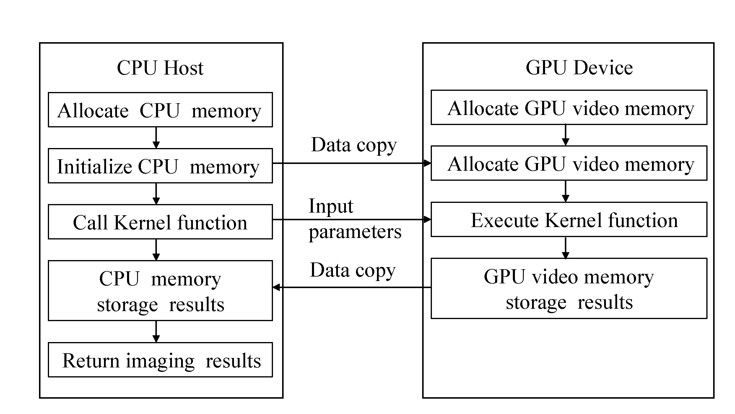
5. Efficient Implementation of the IPML Algorithm Based on the GPU Framework

Although the IPML method introduced in Section 3 could effectively improve the computational efficiency, this was mainly aimed at reducing the calculation amount in the azimuth dimension. In practice, it is necessary to process the data of multiple range cells, and there is still a large amount of data. Considering the engineering implementation of the algorithm, this section proposes an efficient IPML implementation method based on the GPU parallel computing platform. First, the computational complexity of the imaging process for range pulse compression is analyzed. Then, the GPU platform architecture for parallel implementation is outlined, and the parallel optimization process is studied. Finally, the excellent acceleration performance and imaging effect obtained by this method are verified by the experiment data.

5.1. Algorithm Complexity Analysis

The super-resolution imaging algorithm of the RBM is divided into two main stages: one is the echo signal preprocessing stage of the range pulse compression, and the other uses the preprocessed echo signal to realize the IPML super-resolution processing stage. Next, the computational complexity of each stage in the super-resolution imaging process is analyzed in turn.

5.1.1. Range Pulse Compression

In actual engineering, the range pulse compression is completed in the frequency domain. According to the Fast Fourier Transform (FFT) principle, the FFT of the azimuth echo signal to M pulse points requires $M*\left(N/2\right){log}_{2}N$ complex multiplications and $M*N{log}_{2}N$ complex additions; multiplying the echo matrix of the range-dimensional FFT with the frequency-domain function of the matched filtering requires $N*M$ complex multiplications, which inversely transform the result of the two multiplications to the time domain, requiring $M*\left(N/2\right){log}_{2}N$ complex multiplications and $M*N{log}_{2}N$ complex additions. Therefore, the range pulse compression requires a total of $M*N*{log}_{2}N+N*M$ complex multiplications and $2*M*N{log}_{2}N$ complex additions.

5.1.2. Azimuth IPML Super-Resolution

We used the IPML algorithm to perform azimuth super-resolution processing on the echo data after range pulse compression. The steps and calculations required for each iterative deconvolution of each range unit are as follows: the frequency domain calculation convolution requires $\left(M/2\right){log}_{2}M$ complex multiplications and complex additions, and calculating the $\mathbf{y}/\phantom{\mathbf{y}\mathbf{A}{\mathbf{s}}_n}\mathbf{A}{\mathbf{s}}_n$ requires M floating-point multiplications; the frequency domain calculation of ${\mathbf{A}}^T$ and convolution of $\mathbf{y}/\phantom{yA{s}_n}\mathbf{A}{\mathbf{s}}_n$ require $\left(M/2\right){log}_{2}M$ complex multiplications and $M{log}_{2}M$ complex additions, and computing the product of ${\mathbf{s}}_n$ and ${\mathbf{A}}^T\left(\mathbf{y}/\phantom{yA{s}_n}\mathbf{A}{\mathbf{s}}_n\right)$ requires M floating-point multiplications. For N rows of range cells, when the number of iterations is K, the total number of operations is: $4K*N*\left(2*M{log}_{2}M+2*M\right)+2K*N*M$ floating-point multiplications and $2K*N*\left(2*M{log}_{2}M+2*M\right)+8K*N*M{log}_{2}M$ floating-point additions.

5.2. Two-Dimensional Super-Resolution Efficient Implementation

The previous introduction to the CUDA programming architecture and the GPU platform show that the parallel processing of multiunit signals can effectively improve the data processing efficiency by using the relatively independent characteristics of each range unit of the RBM echo [26,27,28]. The efficient implementation of RBM imaging process can be designed in parallel from the three levels of data-receiving, echo preprocessing, and algorithm design.

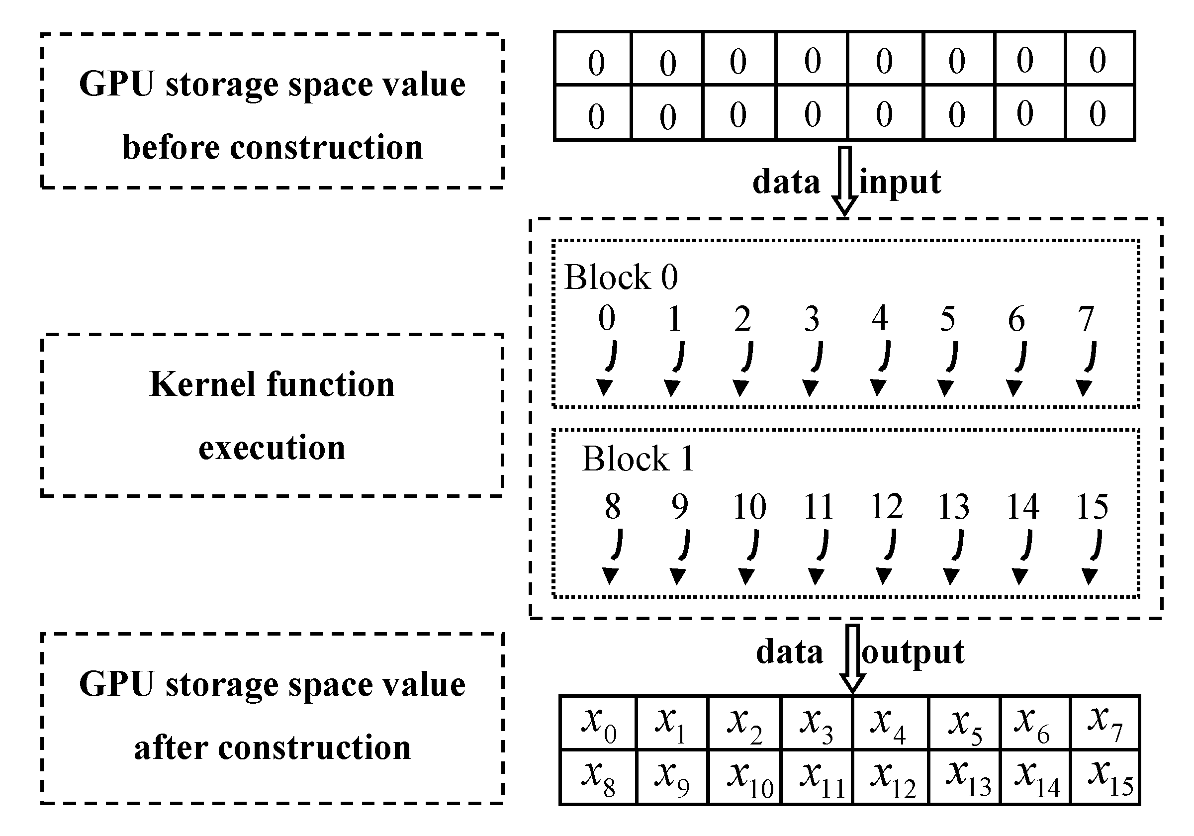
5.2.1. Parallel Implementation of Fourier Transform and Antenna Pattern Preprocessing

During the signal processing of the RBM imaging algorithm, the process of the range pulse compression and azimuth super-resolution involves the Fourier transform, and the azimuth deconvolution of each range unit requires the same antenna pattern to participate. Therefore, these same point Fourier transforms and antenna patterns are pre-stored in the GPU memory or pre-allocated as required by the CPU and GPU resources before the RBM echo signal processing to avoid repeating the same signal processing processes, which can effectively shorten the time required for RBM imaging. The flow chart of the antenna pattern preprocessing is shown in Figure 6, and the specific steps are as follows:

Step 1: RBM antenna pattern reading. We used the CPU to read the original one-dimensional RBM antenna pattern, stored the RBM antenna pattern in the page-locked host memory of the CPU, and then copied the RBM antenna pattern in the page-locked host memory to the global storage unit of the GPU.

Step 2: RBM antenna pattern data type conversion. The RBM antenna pattern was converted into a complex number in parallel on the GPU, the imaginary part was set to zero, and the real part was equal to the value of the original data element.

Step 3: Frequency domain interpolation of the RBM antenna pattern. We performed frequency domain interpolation on the RBM antenna pattern in step 2. In order to ensure that the mainlobe beamwidth of the RBM antenna pattern remained unchanged after interpolation and the sampling rate of the antenna pattern was the same as the azimuth echo sampling rate, a loop iterative multiple interpolation method was added, using the CPU to control the loop process and the GPU to implement the FFT, IFFT, and vector operations.

Step 4: RBM antenna pattern normalization. In the iterative deconvolution process, the antenna pattern needed to be normalized, and the normalization of the antenna pattern was completed in the GPU. An optimization method adapted to parallel reductions was used to solve the maximum value.

Step 5: Dimensional expansion of the RBM antenna pattern. In practice, the interpolated antenna pattern could not match the azimuth echo sampling points, so it was necessary to pad the antenna pattern with zeros at the end of the time domain.

In step 3, the method of the adaptive reduction, which was used to find the maximum value, combined the characteristics of thread asynchronous execution, thread communication, and cooperative synchronization in the CUDA thread block. In the thread block, the communication was realized through shared memory, and the thread block was realized through the barrier method and intrathread synchronization. The maximum value in a series is usually found through traversal comparison. The time complexity is $\mathrm{O}\left(n\right)$, while the time complexity required to use the self-adaptive parallel reduction to find the maximum value is $\mathrm{O}\left({log}_{2}n\right)$. A seven-point vector adaptive parallel reduction was developed to find the maximum value model, as diagrammed in Figure 7.

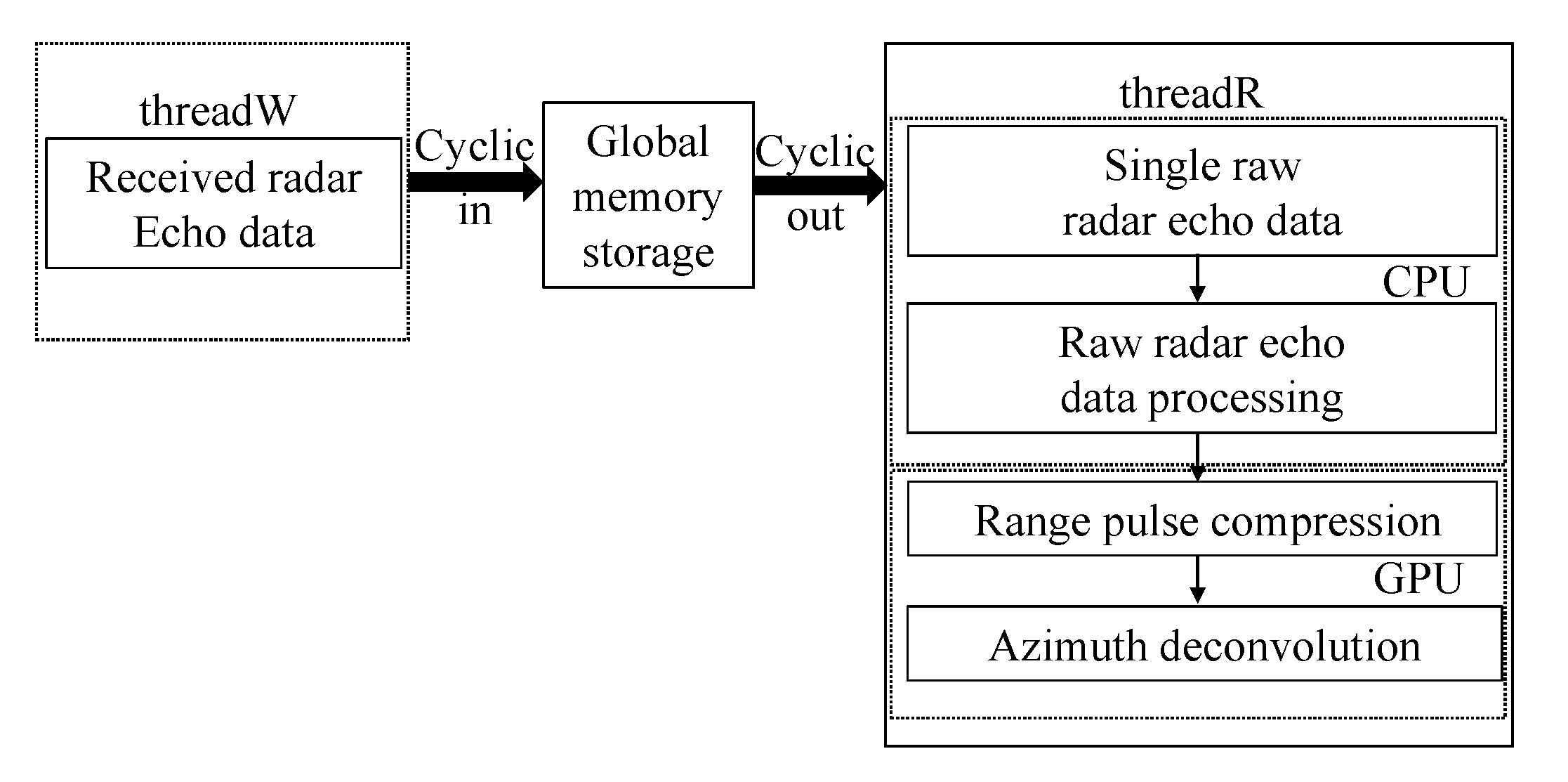
5.2.2. Parallel Realization of the RBM Echo Receiving and Processing

The RBM system is a continuous scanning, continuously receiving echo data, and continuous imaging system mode, with echo data being received for a long time. The total amount of echo data is very large; hence, the linear storage method has insufficient storage space. The circular queue method can simultaneously reuse the allocated storage space, receive the original RBM echo data, and perform signal processing on the RBM echo data. To solve the problem of the echo data processing conflict, the CPU multithread parallel optimization processing method can be used.

Integrating a circular queue into a CPU multithread parallel optimization solver can solve the contradiction between the continuous echo data reception and continuous imaging. According to the theory of CPU multithreading, two CPU threads are created: one CPU thread continuously receives the original RBM echo data by looping them into the queue, denoted as $threadW$, and the other CPU thread reads the original RBM echo data by looping out of the queue, completes the preprocessing of the original RBM echo data, and calls the GPU to implement the RBM echo data signal processing in parallel, which is recorded as $threadR$. After receiving a scan of the RBM echo data, the CPU will complete the preprocessing of the original RBM echo data. In order to realize the communication between the two CPU threads, it is also necessary to create a CPU global memory storage space as a communication platform between the two CPU threads. A flow chart of the echo-data-receiving and processing parallel optimization solver is shown in Figure 8.

5.2.3. Parallel Implementation of the Range Pulse Compression

In actual engineering, range pulse compression is performed in the frequency domain. Combining the characteristics of CPU serial and GPU parallel computing, the CPU thread $threadR$ is used to control the RBM echo signal processing flow, and the GPU is used to realize the RBM echo processing. Giving full play to the respective advantages of CPU and GPU processing greatly improves the processing speed of the RBM echo data and realizes real-time super-resolution imaging.

In the CPU thread $threadR$, the preprocessed RBM echo was copied to the global memory of the GPU; then, the GPU was used to parallelize the pulse compression of the range dimension. The specific steps are as follows:

Step 1: CUDA stream creation. We created two streams, denoted as $Astream$ and $Bstream$; $Astream$ and $Bstream$ were used for the data construction and signal processing control in the range pulse compression, respectively.

Step 2: In $Astream$, we removed the RBM system carrier frequency phase factor matrix $\mathbf{R}$, the matched filtering system spectrum function matrix ${\mathbf{R}}_{MF}$, and frequency domain phase factor matrix ${\mathbf{R}}_{RMC}$ in parallel.

Step 3: When the RBM echo data in the real-number domain were received, the RBM echo in the real-number domain was converted to the complex-number domain in $Bstream$. Then, the Hilbert transform was performed on the RBM echo in the complex-number domain so that the RBM echo matrix could obtain the range and azimuth phase information, which is denoted as ${\mathbf{E}}_{hilbert}$. The matrix dot multiplication of ${\mathbf{E}}_{hilbert}$ and $\mathbf{R}$ was implemented in the time domain to realize the removal of the system carrier frequency phase factor in the RBM echo. The RBM echo matrix obtained after removing the carrier frequency is denoted as ${\mathbf{E}}_R$.

Step 4: We took the range dimension FFT of the matrix ${\mathbf{E}}_R$ using the Fourier transform scheme $FF{T}_{M\left(N\right)}$. We conducted dot-multiply operations on matrix ${\mathbf{R}}_{MF}$ and ${\mathbf{R}}_{RMC}$ and then performed range dimension IFFT to realize the range pulse compression. The RBM echo matrix obtained after the range pulse compression is denoted as ${\mathbf{E}}_{RMC}$.

The serial CPU method could also be used to realize the construction of matrices $\mathbf{R}$ and ${\mathbf{R}}_{MF}$, but its computational complexity was $\mathrm{O}\left(n^2\right)$, while, when using the GPU parallel implementation, its computational complexity was $\mathrm{O}\left(1\right)$, and the execution efficiency was improved to $n^2$. A schematic diagram of the principle of the GPU implementation of the matrix construction is shown in Figure 9, describing the execution process of each thread block and thread. Assuming that the input GPU storage space values were all initialized to 0, the size of the kernel function was $\left(2,0,0\right)$, and the size of each thread block was $\left(8,0,0\right)$; during the execution of the kernel function, the threads between the thread blocks were executed synchronously. The threads in the thread block were executed asynchronously, and 16 threads in the grid concurrently executed the kernel function to construct the matrix elements once to complete the elements in the matrix structure. Using the traditional serial method, we realized the point multiplication of two matrices with a computational complexity of $\mathrm{O}\left(n^2\right)$; taking advantage of the parallel computing advantages of the GPU super multicore and super multithreading, the time complexity of the matrix point multiplication was reduced to $\mathrm{O}\left(1\right)$.

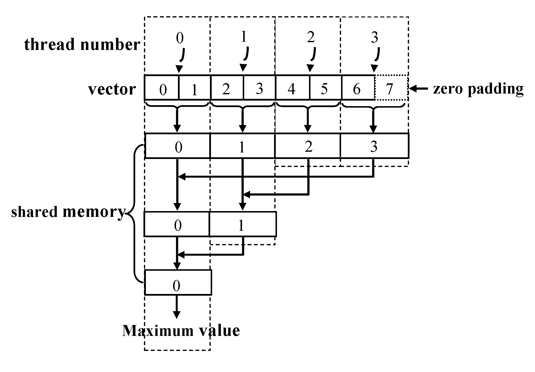
5.2.4. Parallel Implementation of the IPML Super-Resolution Algorithm

In order to implement the IPML super-resolution imaging algorithm in parallel on the GPU, the algorithm needed to be optimized for the parallel computing mode of the GPU. The specific parallel implementation steps of IPML super-resolution imaging algorithm are as follows:

Step 1: We used the method of combining the parallel matrix transposition and the complex amplitude solution to realize the transposition of the RBM echo matrix ${\mathbf{E}}_{RMC}$ after the range pulse compression, and the solved amplitude of ${\mathbf{E}}_{RMC}$ was stored in the GPU global memory in the order of the range rows. The matrix after transposing and solving the magnitude was recorded as $\left|{{\mathbf{E}}^T}_{RMC}\right|$, and the iterative deconvolution input matrix ${\mathbf{s}}^0\left(N,M\right)$ was initialized as $\left|{{\mathbf{E}}^T}_{RMC}\right|$.

Step 2: When the number of iterations $j>2$, and j was a positive integer, we added a vector factor ${\lambda }_N^j$ to ensure that the deconvolution algorithm performed stably; the length of the vector ${\lambda }_N^j$ was the number of sampling points in the range dimension, and the nth element of ${\lambda }_N^j\left(n\right)$ was obtained by the following expression:

$$\begin{array}{c}\hfill \begin{array}{c}{\lambda }_N^j\left(n\right)=max(m\mathrm{in}({\Delta \mathbf{K}}_1^{j-1}{\left(N,M\right)}_n.*{\Delta \mathbf{K}}_2^{j-1}{\left(N,M\right)}_n\hfill \\ /({\Delta \mathbf{K}}_2^{j-1}{\left(N,M\right)}_n.*{\Delta \mathbf{K}}_2^{j-1}{\left(N,M\right)}_n+\epsilon ),1),0)\hfill \end{array},\end{array}$$

(20)

where $.*$ represents the vector dot-product operation, j represents the deconvolution of the jth iteration, $\epsilon$ represents an infinitesimal quantity, which takes $\epsilon ={10}^{-12}$ in practical engineering, ${\Delta \mathbf{K}}_1^{j-1}{(N,M)}_n$ is a vector composed of elements in the nth range row of the error matrix in the $\left(j-1\right)$th iteration, ${\Delta \mathbf{K}}_2^{j-1}{(N,M)}_n$ is a vector composed of elements of the nth range row of the error matrix in the $\left(j-1\right)$th iteration, and the solutions of the error matrix ${\Delta \mathbf{K}}_1^{j-1}(N,M)$ and ${\Delta \mathbf{K}}_2^{j-1}(N,M)$ are as follows:

$$\begin{array}{c}\hfill \begin{array}{c}{\Delta \mathbf{K}}_1^{j-1}\left(N,M\right)={\mathbf{s}}^{j-1}\left(N,M\right)-{\mathbf{Y}}^{j-1}\left(N,M\right)\end{array},\end{array}$$

(21)

$$\begin{array}{c}\hfill \begin{array}{c}{\Delta \mathbf{K}}_2^{j-1}\left(N,M\right)={\mathbf{s}}^{j-2}\left(N,M\right)-{\mathbf{Y}}^{j-2}\left(N,M\right)\end{array},\end{array}$$

(22)

where the matrices ${\mathbf{Y}}^{j-1}\left(N,M\right)$ and ${\mathbf{Y}}^{j-2}\left(N,M\right)$ are the $\left(j-1\right)$th and $\left(j-2\right)$th iterative deconvolution results after processing in the positive constraints, respectively. The matrices ${\mathbf{s}}^{j-1}\left(N,M\right)$ and ${\mathbf{s}}^{j-2}\left(N,M\right)$ are the results of the $\left(j-1\right)$th and $\left(j-2\right)$th iterative deconvolution, respectively.

Step 3: We conducted positive constraint processing on the input matrix ${\mathbf{s}}^{j-1}\left(N,M\right)$ of the jth iterative deconvolution; the processed result was ${\mathbf{Y}}^j\left(N,M\right)$, and the vector composed of elements of the nth range row of the matrix ${\mathbf{Y}}^j\left(N,M\right)$ was:

$$\begin{array}{c}\hfill \begin{array}{c}{\mathbf{Y}}^j{\left(N,M\right)}_n=max({\mathbf{s}}^{j-1}{(N,M)}_n+{\lambda }_N^j\left(n\right)\hfill \\ \times ({\mathbf{s}}^{j-1}{(N,M)}_n-s^{j-2}{(N,M)}_n),0)\hfill \end{array},\end{array}$$

(23)

where the vectors ${\mathbf{s}}^{j-1}{\left(N,M\right)}_n$ and ${\mathbf{s}}^{j-2}{\left(N,M\right)}_n$ were the results of the $\left(j-1\right)$th and $\left(j-2\right)$th iterative deconvolution, respectively.

Step 4: We calculated the convolution kernel matrix $\mathbf{C}\left(N,M\right)$, which was obtained by the following formula:

$$\begin{array}{c}\hfill \begin{array}{c}{\mathbf{C}}^j\left(N,M\right)=\left|{{\mathbf{E}}^T}_{RMC}\right|./\left(real\right(IFF{T}_{N\left(M\right)}({\mathbf{A}}_{fft}(N,M)\hfill \\ .*FF{T}_{N\left(M\right)}\left({\mathbf{Y}}^j(N,M)\right)\left)\right)+\epsilon )+\epsilon \hfill \end{array},\end{array}$$

(24)

where $.*$ represents the matrix point multiplication operation, $./$ represents the matrix point division operation, $FF{T}_{N\left(M\right)}\left(\mathbf{X}\right)$ and $IFF{T}_{N\left(M\right)}\left(\mathbf{X}\right)$ represent the performing FFT and IFFT on the range rows of the matrix $\mathbf{X}$, respectively, $real\left(\mathbf{X}\right)$ represents taking the real part of each complex element in the matrix $\mathbf{X}$, and ${\mathbf{A}}_{fft}(N,M)$ is the antenna pattern matrix after the FFT.

Step 5: We output the deconvolution result of ${\mathbf{s}}^j\left(N,M\right)$ and calculated the iterative error matrix ${\Delta \mathbf{K}}_1^j(N,M)$ and ${\Delta \mathbf{K}}_2^j(N,M)$ at the same time; ${\Delta \mathbf{K}}_1^j(N,M)$, ${\mathbf{s}}^{\mathbf{j}}\left(N,M\right)$, and ${\Delta \mathbf{K}}_2^j(N,M)$ were solved by the following formulas, respectively:

$$\begin{array}{c}\hfill \begin{array}{c}\begin{array}{c}{\mathbf{s}}^j\left(N,M\right)=max({\mathbf{Y}}^j(N,M)\hfill \\ .*real\left(IFF{T}_{N\left(M\right)}({\mathbf{A}}_{fftconj}(N,M).*{\mathbf{C}}^j(N,M))\right),0)\hfill \end{array}\end{array},\end{array}$$

(25)

$$\begin{array}{c}\hfill \begin{array}{c}{\Delta \mathbf{K}}_1^j\left(N,M\right)={\mathbf{s}}^j\left(N,M\right)-{\mathbf{Y}}^j\left(N,M\right)\end{array},\end{array}$$

(26)

$$\begin{array}{c}\hfill \begin{array}{c}{\Delta \mathbf{K}}_2^j\left(N,M\right)={\Delta \mathbf{K}}_1^{j-1}\left(N,M\right)\end{array},\end{array}$$

(27)

where ${\mathbf{A}}_{fftconj}(N,M)$ is the conjugate matrix of ${\mathbf{A}}_{fft}(N,M)$.

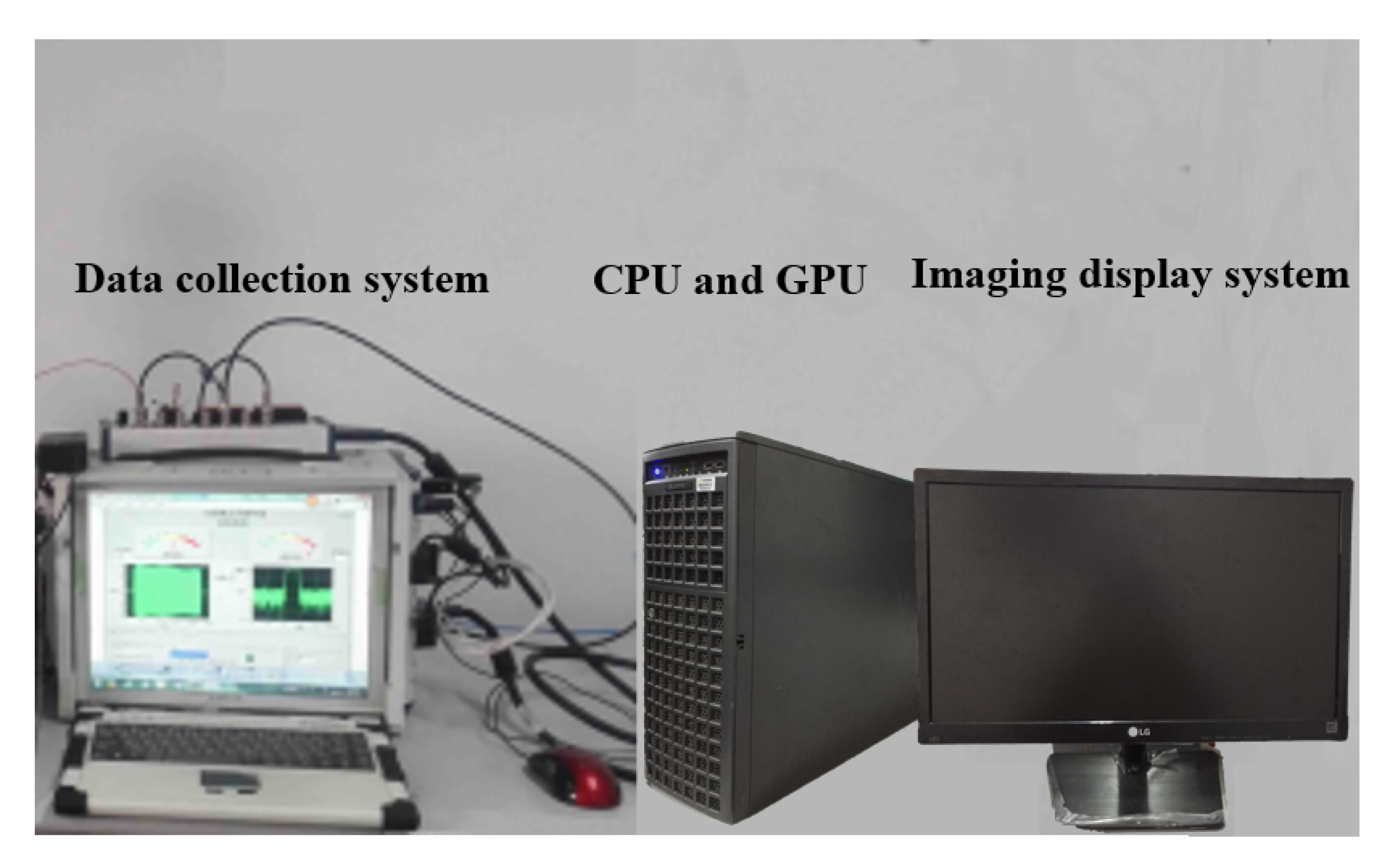
5.3. Experiment Data Verification

5.3.1. Imaging Performance Analysis

In real-time super-resolution imaging, it was necessary to ensure the speed of the radar signal processing and the image quality of the imaging results. In order to verify the correctness, validity, and high quality of the imaging results implemented in parallel by the GPU-based RBM super-resolution imaging algorithm, under the condition of the same RBM echo, we compared the imaging results of the serial processing by Matlab and the parallel processing by the GPU, and used the absolute value error as the judgment standard. The RBM system and GPU server platform are shown in Figure 10. The RBM imaging system software ran on the server computer, and the RBM echo data were transmitted to the server computer through the local area network in real time. The CPU model was an Intel (R) CPU E5-2690 v2 @3.00 GHz, and the graphics processor was an NVIDIA Tesla K40c.

In order to verify the effectiveness of the proposed parallel processing structure in this section, we carried out the verification experiment with the RBM experiment data in Section 4. The size of the RBM experiment data matrix was 1801 * 257 (range * azimuth), and the calculation formula of the absolute value error was:

$$\begin{array}{c}\hfill \begin{array}{c}\Delta \xi =\left|\mathbf{M}-\mathbf{G}\right|\end{array},\end{array}$$

(28)

where $\mathbf{M}$ represents the result of the serial processing by Matlab, and $\mathbf{G}$ represents the result of the parallel processing by the GPU. The mean error of the absolute value error was defined as:

$$\begin{array}{c}\hfill \begin{array}{c}\Delta \overline{\xi }=\Delta \xi N*M\end{array},\end{array}$$

(29)

where M was the number of range rows, and N was the number of azimuth echoes.

The imaging results of the Matlab method and the GPU method are shown in Figure 11. Figure 11a and Figure 11b represent the processing results by the Matlab method and the GPU method, respectively. The two boats can be distinguished and the azimuth resolution is greatly improved. After calculation, the absolute error between the Matlab serial implementation method and the GPU parallel implementation method also tended toward zero, and the absolute mean error was 0.0016. Combining Figure 11a,b illustrates the correctness of the signal processing process, implemented in parallel by the entire GPU.

5.3.2. Speedup Ratio Analysis

In order to verify the performance of the IPML super-resolution imaging method under the GPU framework, this section compares the results of the parallel processing with the GPU and the serial processing with the CPU. The serial method based on Matlab and the parallel implementation method based on the GPU were used to separately process the RBM echo data of different scales.

Table 3. Comparison of the execution time between the serial method implemented by Matlab and the parallel method implemented by the GPU (unit: ms).

Echo Size (Range * Azimuth)	Matlab	GPU	Speedup Ratio
1024 * 1024	4411	37	119
1024 * 2048	7824	58	135
2048 * 2048	16,659	100	167
2048 * 4096	28,294	230	123
4096 * 4096	54,529	455	120
4096 * 8192	104,967	961	109
8192 * 8192	205,350	2151	95

compares the time taken by the two methods to process RBM echoes of different sizes with 15 deconvolution iterations.

In Table 3, the speedup ratio is defined as the ratio of the time used by Matlab to the time used by the GPU. From the test results, the parallel implementation method of the super-resolution imaging algorithm based on the GPU had an extremely high execution efficiency; the execution speed was improved by nearly 100 times. Therefore, the parallel implementation method based on the GPU is very suitable for real-time RBM super-resolution imaging.

6. Conclusions

This paper focused on the research hotspot of the angular resolution of real beam mapping (RBM) imagery. For the Poisson distribution model, the IPML method based on the adaptive iterative acceleration factor significantly improved the iterative operation efficiency of the super-resolution maximum likelihood algorithm. In addition, this paper proposed a parallel processing architecture for the super-resolution imaging method, using GPU multithreading, multicomputing unit hardware architecture, and the parallel optimization of RBM imaging. It was verified that the acceleration ratio of the parallel processing method was about 100 times that of the traditional super-resolution algorithm, which meets the needs of general real-time imaging applications in practical engineering.

References

1. Nekrasov, A.; Dell’Acqua, F. Airborne Weather Radar: A theoretical approach for water-surface backscattering and wind measurements. IEEE Geosci. Remote Sens. Mag. 2016, 4, 38–50. [Google Scholar] [CrossRef]
2. Gambardella, A.; Migliaccio, M. On the superresolution of microwave scanning radiometer measurements. IEEE Geosci. Remote Sens. Lett. 2008, 5, 796–800. [Google Scholar] [CrossRef]
3. Li, X.; He, J.; He, Z.; Zeng, Q. Weather radar range and angular super-resolution reconstruction technique on oversampled reflectivity data. J. Inf. Comput. Sci. 2011, 8, 2553–2562. [Google Scholar]
4. Zhang, Y.; Luo, J.; Li, J.; Mao, D.; Zhang, Y.; Huang, Y.; Yang, J. Fast inverse-scattering reconstruction for airborne high-squint radar imagery based on Doppler centroid compensation. IEEE Trans. Geosci. Remote Sens. 2021, 60, 5205517. [Google Scholar] [CrossRef]
5. Yang, L.; Bi, G.; Xing, M.; Zhang, L. Airborne SAR moving target signatures and imagery based on LVD. IEEE Trans. Geosci. Remote Sens. 2015, 53, 5958–5971. [Google Scholar] [CrossRef]
6. Long, T.; Lu, Z.; Ding, Z.; Liu, L. A DBS Doppler centroid estimation algorithm based on entropy minimization. IEEE Trans. Geosci. Remote Sens. 2011, 49, 3703–3712. [Google Scholar] [CrossRef]
7. Rigelsford, J. Introduction to Airborne Radar. Sens. Rev. 2002, 22, 265–266. [Google Scholar]
8. Candès, E.J.; Fernandez-Granda, C. Towards a mathematical theory of super-resolution. Commun. Pure Appl. Math. 2014, 67, 906–956. [Google Scholar] [CrossRef] [Green Version]
9. Sementilli, P.; Hunt, B.R.; Nadar, M. Analysis of the limit to superresolution in incoherent imaging. JOSA A 1993, 10, 2265–2276. [Google Scholar] [CrossRef]
10. Piles, M.; Camps, A.; Vall-Llossera, M.; Talone, M. Spatial-resolution enhancement of SMOS data: A deconvolution-based approach. IEEE Trans. Geosci. Remote Sens. 2009, 47, 2182–2192. [Google Scholar] [CrossRef]
11. Sethmann, R.; Burns, B.A.; Heygster, G.C. Spatial resolution improvement of SSM/I data with image restoration techniques. IEEE Trans. Geosci. Remote Sens. 1994, 32, 1144–1151. [Google Scholar] [CrossRef]
12. Álvarez-Pérez, J.L.; Marshall, S.J.; Gregson, K. Resolution improvement of ERS scatterometer data over land by Wiener filtering. Remote Sens. Environ. 2000, 71, 261–271. [Google Scholar] [CrossRef]
13. Zhang, Q.; Zhang, Y.; Huang, Y.; Zhang, Y.; Pei, J.; Yi, Q.; Li, W.; Yang, J. TV-sparse super-resolution method for radar forward-looking imaging. IEEE Trans. Geosci. Remote Sens. 2020, 58, 6534–6549. [Google Scholar] [CrossRef]
14. Calvetti, D.; Morigi, S.; Reichel, L.; Sgallari, F. Tikhonov regularization and the L-curve for large discrete ill-posed problems. J. Comput. Appl. Math. 2000, 123, 423–446. [Google Scholar] [CrossRef] [Green Version]
15. Schmidt, R. Multiple emitter location and signal parameter estimation. IEEE Trans. Antennas Propag. 1986, 34, 276–280. [Google Scholar] [CrossRef] [Green Version]
16. Zhang, Y.; Li, W.; Zhang, Y.; Huang, Y.; Yang, J. A fast iterative adaptive approach for scanning radar angular superresolution. IEEE J. Sel. Top. Appl. Earth Obs. Remote Sens. 2015, 8, 5336–5345. [Google Scholar] [CrossRef]
17. Sadjadi, F. Radar beam sharpening using an optimum FIR filter. Circuits Syst. Signal Process. 2000, 19, 121–129. [Google Scholar] [CrossRef]
18. Suzuki, T. Radar beamwidth reduction techniques. IEEE Aerosp. Electron. Syst. Mag. 1998, 13, 43–48. [Google Scholar] [CrossRef]
19. Zhang, Y.; Tuo, X.; Huang, Y.; Yang, J. A TV forward-looking super-resolution imaging method based on TSVD strategy for scanning radar. IEEE Trans. Geosci. Remote Sens. 2020, 58, 4517–4528. [Google Scholar] [CrossRef]
20. Tuo, X.; Zhang, Y.; Huang, Y.; Yang, J. Fast sparse-TSVD super-resolution method of real aperture radar forward-looking imaging. IEEE Trans. Geosci. Remote Sens. 2020, 59, 6609–6620. [Google Scholar] [CrossRef]
21. Lenti, F.; Nunziata, F.; Migliaccio, M.; Rodriguez, G. Two-dimensional TSVD to enhance the spatial resolution of radiometer data. IEEE Trans. Geosci. Remote Sens. 2013, 52, 2450–2458. [Google Scholar] [CrossRef]
22. Shea, J.D.; Van Veen, B.D.; Hagness, S.C. A TSVD analysis of microwave inverse scattering for breast imaging. IEEE Trans. Biomed. Eng. 2011, 59, 936–945. [Google Scholar] [CrossRef] [Green Version]
23. Ly, C.; Dropkin, H.; Manitius, A.Z. Extension of the music algorithm to millimeter-wave (mmw) real-beam radar scanning antennas. In Proceedings of the Radar Sensor Technology and Data Visualization, Orlando, FL, USA, 1–4 April 2002; SPIE: Bellingham, WA, USA, 2002; Volume 4744, pp. 96–107. [Google Scholar]
24. Uttam, S.; Goodman, N.A. Superresolution of coherent sources in real-beam data. IEEE Trans. Aerosp. Electron. Syst. 2010, 46, 1557–1566. [Google Scholar] [CrossRef]
25. Zhang, Y.; Jakobsson, A.; Yang, J. Range-recursive IAA for scanning radar angular super-resolution. IEEE Geosci. Remote Sens. Lett. 2017, 14, 1675–1679. [Google Scholar] [CrossRef]
26. Strnad, D.; Nerat, A. Parallel construction of classification trees on a GPU. Concurr. Comput. Pract. Exp. 2016, 28, 1417–1436. [Google Scholar] [CrossRef]
27. Mao, D.; Zhang, Y.; Zhang, Y.; Huang, Y.; Yang, J. Realization of airborne forward-looking radar super-resolution algorithm based on GPU frame. In Proceedings of the 2016 IEEE CIE International Conference on Radar (RADAR), Guangzhou, China, 10–13 October 2016; pp. 1–5. [Google Scholar]
28. Corporation, N. CUDA C Programming Guide; NVIDIA: Santa Clara, CA, USA, 2017. [Google Scholar]
29. Guan, J.; Huang, Y.; Yang, J.; Li, W.; Wu, J. Improving angular resolution based on maximum a posteriori criterion for scanning radar. In Proceedings of the 2012 IEEE Radar Conference, Atlanta, GA, USA, 7–11 May 2012; pp. 451–454. [Google Scholar]
30. Li, D.; Li, Y.; Wang, L.; Zhong, Y.; Yan, K. Improved Landweber Iteration-Based Angular Superresolution for Airborne Forward-Looking Radar. ICIC Express Lett. Part B Appl. Int. J. Res. Surv. 2017, 8, 1121–1126. [Google Scholar]
31. Tan, X.; Roberts, W.; Li, J.; Stoica, P. Sparse learning via iterative minimization with application to MIMO radar imaging. IEEE Trans. Signal Process. 2010, 59, 1088–1101. [Google Scholar] [CrossRef]
32. Xu, G.; Xing, M.; Zhang, L.; Liu, Y.; Li, Y. Bayesian inverse synthetic aperture radar imaging. IEEE Geosci. Remote Sens. Lett. 2011, 8, 1150–1154. [Google Scholar] [CrossRef]
33. Guan, J.; Yang, J.; Huang, Y.; Li, W. Maximum a posteriori–based angular superresolution for scanning radar imaging. IEEE Trans. Aerosp. Electron. Syst. 2014, 50, 2389–2398. [Google Scholar] [CrossRef]
34. Tan, K.; Li, W.; Huang, Y.; Yang, J. Dual-channel fast iterative shrinkage-thresholding regularization algorithm for scanning radar forward-looking imaging. J. Appl. Remote Sens. 2017, 11, 015008. [Google Scholar] [CrossRef]
35. Tai, X.C.; Wu, C. Augmented Lagrangian method, dual methods and split Bregman iteration for ROF model. In Proceedings of the International Conference on Scale Space and Variational Methods in Computer Vision, Voss, Norway, 1–5 June 2009; Springer: Berlin/Heidelberg, Germany, 2009; pp. 502–513. [Google Scholar]
36. Li, P.; Bu, J.; Yu, J.; Chen, C. Towards robust subspace recovery via sparsity-constrained latent low-rank representation. J. Vis. Commun. Image Represent. 2016, 37, 46–52. [Google Scholar] [CrossRef]
37. Zhang, Y.; Luo, J.; Zhang, Y.; Huang, Y.; Cai, X.; Yang, J.; Mao, D.; Li, J.; Tuo, X.; Zhang, Y. Resolution Enhancement for Large-Scale Real Beam Mapping Based on Adaptive Low-Rank Approximation. IEEE Trans. Geosci. Remote Sens. 2022, 60, 5116921. [Google Scholar] [CrossRef]
38. Migliaccio, M.; Gambardella, A. Microwave radiometer spatial resolution enhancement. IEEE Trans. Geosci. Remote Sens. 2005, 43, 1159–1169. [Google Scholar] [CrossRef]
39. Early, D.S.; Long, D.G. Image reconstruction and enhanced resolution imaging from irregular samples. IEEE Trans. Geosci. Remote Sens. 2001, 39, 291–302. [Google Scholar] [CrossRef] [Green Version]
40. Holmes, T.J.; Liu, Y.H. Acceleration of maximum-likelihood image restoration for fluorescence microscopy and other noncoherent imagery. JOSA A 1991, 8, 893–907. [Google Scholar] [CrossRef]
41. Biggs, D.S.; Andrews, M. Acceleration of iterative image restoration algorithms. Appl. Opt. 1997, 36, 1766–1775. [Google Scholar] [CrossRef] [Green Version]
42. Singh, M.K.; Tiwary, U.S.; Kim, Y.H. An adaptively accelerated Lucy-Richardson method for image deblurring. EURASIP J. Adv. Signal Process. 2007, 2008, 365021. [Google Scholar] [CrossRef] [Green Version]
43. Huang, Y.; Zha, Y.; Wang, Y.; Yang, J. Forward looking radar imaging by truncated singular value decomposition and its application for adverse weather aircraft landing. Sensors 2015, 15, 14397–14414. [Google Scholar] [CrossRef] [Green Version]
Figure 1. Antenna pattern and target scene. (a) Antenna pattern. (b) Target distribution scene.
Remotesensing 15 01164 g001
Figure 2. RBM echo and super-resolution processing results with different methods. (a) RBM raw echo in SNR = 30 dB. (b) The processing result using the REGU method. (c) The processing result using the TV method. (d) The processing result using the TSVD method. (e) The processing result using the PML method. (f) The processing result using the IPML method.
Remotesensing 15 01164 g002
Figure 3. RBM echo and super-resolution processing results using different methods. (a) RBM raw echo in SNR = 10 dB. (b) The processing result using the REGU method. (c) The processing result using the TV method. (d) The processing result using the TSVD method. (e) The processing result using the PML method. (f) The processing result using the IPML method.
Remotesensing 15 01164 g003
Figure 4. Real data processing results with different methods. (a) Optical scenario. (b) RBM raw echo. (c) The processing result using the REGU method. (d) The processing result using the TSVD method. (e) The processing result using the PML method. (f) The processing result using the IPML method.
Remotesensing 15 01164 g004
Figure 5. Iterative process mean square error curve. (a) PML. (b) IPML.
Remotesensing 15 01164 g005
Figure 6. Antenna pattern preprocessing flowchart.
Remotesensing 15 01164 g006
Figure 7. Model diagram of the point vector adaptive reduction parallel maximization.
Remotesensing 15 01164 g007
Figure 8. Parallel optimization of the radar echo data receiving and processing.
Remotesensing 15 01164 g008
Figure 9. Schematic diagram of the 2 * 8 matrix parallel construction method.
Remotesensing 15 01164 g009
Figure 10. The RBM system and the GPU server platform.
Remotesensing 15 01164 g010
Figure 11. Experiment data processing results. (a) The processing result using Matlab. (b) The processing results obtained using the GPU.
Remotesensing 15 01164 g011