Sea Surface Temperature Gradients Estimation Using Top-of-Atmosphere Observations from the ESA Earth Explorer 10 Harmony Mission: Preliminary Studies

Abstract

The Harmony satellite mission was recently approved as the next European Space Agency (ESA) Earth Explorer 10. The mission science objectives cover several applications related to solid earth, the cryosphere, upper-ocean dynamics and air–sea interactions. The mission consists of a constellation of two satellites, flying with the Copernicus Sentinel 1 (C or D) spacecraft, each hosting a C-band receive-only radar and a thermal infrared (TIR) payload. From an ocean dynamics/air–sea interaction perspective, the mission will provide the unique opportunity to observe simultaneously the signature of submesoscale upper-ocean processes via synthetic aperture radar and TIR imagery. The TIR imager is based on microbolometer technology and its acquisitions will rely on four channels: three narrow-band channels yielding observations at a ≃1 km spatial sampling distance (SSD) and a panchromatic (PAN, 8–12 $\mathsf{\mu }$m) channel characterized by a ≃300 m SSD. Our study investigates the potential of Harmony in retrieving spatial features related to sea surface temperature (SST) gradients from the high-resolution PAN channel, relying on top-of-atmosphere (TOA) observations. Compared to a standard SST gradient retrieval, our approach does not require atmospheric correction, thus avoiding uncertainties due to inter-channel co-registration and radiometric consistency, with the possibility of exploiting the higher resolution of the PAN channel. The investigations were carried out simulating the future Harmony TOA radiances (TARs), as well as relying on existing state-of-the-art level 1 satellite products. Our approach enables the correct description of SST features at the sea surface avoiding the generation of spurious features due to atmospheric correction and/or instrumental issues. In addition, analyses based on existing satellite products suggest that the clear-sky TOA observations, in a typical mid-latitude scene, allow the reconstruction of up to 85% of the gradient magnitudes found at the sea-surface level. The methodology is less efficient in tropical areas, suffering from smoothing effects due to the high concentrations of water vapor.

1. General Introduction and Background

Sea surface temperature (SST) gradients are intimately linked with the ocean and the lower atmosphere dynamics. SST gradients can result from different processes, such as the following: (i) the encounter of water masses of different remote origins, e.g., in frontal areas, such as those observed along the Antarctic Circumpolar Current or associated with the major western boundary currents [1,2]; (ii) the processes that modify locally the upper-ocean heat content, for example, through vertical advection [3] and mixing driven by mesoscale and submesoscale features [4]; (iii) through localized momentum and energy exchanges caused by the interaction with the overlying atmosphere [5,6]. The air–sea interface is where the response of the ocean slowly integrates the temporal atmospheric variance but also where the atmosphere quickly responds to the spatial variance in the oceanic fields [7,8]. In fact, SST gradients’ connection with local changes in sea surface roughness and surface wind speed, up to the modulation of storm tracks, has been documented several times in the scientific literature, e.g., [9,10,11,12]. In addition, particularly in coastal seas, frontal regions (well-depicted by SST gradient patterns) are often the signature of upwelling systems that are known to play a primary role in the functioning of marine ecosystems, leading to enhanced primary production, with relevant impacts up to the higher trophic layers [3,13]. The accurate retrieval of SST gradients is thus crucial to correctly investigate several different processes, and it was thus the subject of specific studies dedicated to the quality assessment of single/multi-sensor (level 3, L3) and interpolated (level 4, L4) SST products, based on in situ approaches [14,15]. Moreover, the satellite-derived SST gradients/patterns recently turned out to be crucial also for other practical applications, such as the improvement of the altimeter-derived surface geostrophic currents distributed within the Copernicus Marine Service, as well as for space-based sea surface salinity monitoring. SST can indeed provide constraints to optimize and enhance the effective spatial resolution of satellite products related to the ocean physical component [16,17,18,19,20,21]. The accurate retrieval of SST and/or SST gradients, together with other oceanic, atmospheric and land variables, is also driving the design of future satellite missions developed by the European Space Agency (ESA). For instance, the future Copernicus Imaging Microwave Radiometer (CIMR) mission aims at retrieving an all-weather SST with almost total daily coverage (subdaily in polar areas) and spatial resolutions around 15 km (https://cimr.eu/node/104, accessed on 3 November 2022). In the framework of the mission evaluation studies, it was shown that the CIMR will significantly contribute to the SST gradients retrieval in dynamically active oceanic regions, such as the Gulf Stream or the Agulhas retroflection region [22]. SST gradients are among the target quantities that shall be retrieved by the ESA Harmony satellite mission (Earth Explorer 10) with the aim of closely investigating the link between SST and the lower atmospheric dynamics at a fine scale [23]. The present study is aimed at illustrating a strategy to optimize the SST gradients’ retrieval within the context of the Harmony mission. The manuscript is structured as follows:

• Section 1 and Section 2 provide an overview of the Harmony mission and present the main issues intrinsic with the standard SST gradients’ retrieval via a dedicated numerical study;
• Section 3 presents the main methodologies and data used for our investigations;
• Section 4 and Section 5 illustrate our main findings and the main conclusions/perspectives of the study.

SST Gradients’ Retrieval: Context and Motivation of the Proposed Approach

The ESA Harmony mission science objectives cover a wide range of applications: from upper-ocean dynamics, to air–sea interactions, to the cryosphere and solid earth, aiming to improve our understanding of the dynamic processes associated with surface stress and relative motions at the Earth’s surface. Regarding the ocean applications, the mission is designed to support the study of coupled atmosphere–ocean dynamics. This is tackled focusing on air–sea interactions and upper-ocean processes in the submesoscale to mesoscale dynamical regimes, which are crucial for the mixing and transport of momentum, heat, carbon, nutrients and marine organisms. These processes generally have a clear signature in both sea surface roughness and sea surface temperature (SST gradients), the latter being actively involved in the coupling process itself. In order to achieve the scientific objectives of the mission, Harmony’s concept consists of flying, in a configurable formation with the Copernicus Sentinel-1 C or D, two satellites, each hosting one C-band receive-only radar instrument and one thermal infrared (TIR) payload [24]. The TIR payload will provide multi-angular observations of the same area observed by the C-band radar: a ≃30${}^{\circ }$ off-nadir swath approximately 250 km wide (the C-band radar will provide observations based on synthetic aperture radar (SAR) interferometry). The acquisition over the ocean will be limited to target areas of interest for air–sea interaction studies (e.g., the Gulf Stream, the Agulhas retroflection region and the equatorial band [23,25]). Given the constraints of the overall platform, the TIR imager payload will be based on microbolometer technology.

Table 1. Relevant characteristics of the Harmony TIR imager channels and, for reference, the Sentinel 3 SLSTR equivalent to TIR-1 and TIR-2. For the Harmony NE$\Delta$T, “G” and “T”, respectively, stand for goal and threshold. For the SLSTR NE$\Delta$T, “R” and “IF”, respectively, stand for requirement and in-flight performance value, following [26]. In this table, WL = wavelength, SSD = spatial sampling distance, NE$\Delta$T = noise-equivalent $\Delta$ temperature.

HARMONY	Central WL	Width	SSD	NE$\Delta$T @ 280 K	Rad. Accuracy @ 280 K
Channel	($\mathsf{\mu }$m)	($\mathsf{\mu }$m)	(km)	(K)	(K)
TIR-1	10.85	0.9	1	0.1(G)–0.15(T)	0.5
TIR-2	11.95	1.1	1	0.1(G)–0.15(T)	0.5
CD-1	8.6	1.2	1	0.1(G)–0.15(T)	0.5
PAN	10.0	4.0	0.33	0.1(G)–0.15(T)	0.5
S3-SLSTR	Central WL	Width	SSD	NE$\Delta$T @ 266 K	Rad. Accuracy @265-310K
Channel	($\mathsf{\mu }$m)	($\mathsf{\mu }$m)	(km)	(K)	(K)
S8	10.85	0.9	1	0.050(R)–(0.014)(IF)	<0.1
S9	12.00	1.0	1	0.05(R)–(0.022)(IF)	<0.1

reports the preliminary requirements for this payload [23,25] relevant for this study.

The proposed configuration includes the following:

• The channels TIR-1 and TIR-2 for the estimation of the SST and optically thin cirrus cloud detection (e.g., [27]);
• The channel CD-1 for cloud detection ([28]);
• The panchromatic (PAN) broadband channel for spatial feature extraction (i.e., cloud motion winds).

Compared to present-day state-of-the art satellite missions for SST retrieval (e.g., Sentinel-3 Sea and Land Surface Temperature Radiometer—SLSTR sensor), the radiometric performances of the Harmony TIR payload are sub-optimal, mainly due to technological/budget constraints (see Table 1). Moreover, comparing the Harmony TIR channels NE$\Delta$T with the ones of other missions operating in the TIR band yields ratios of about 3 for Landsat-8, 5 for VIIRS (Visible Infrared Imaging Radiometer Suite) and 2 for SEVIRI (Spinning Enhanced Visible and Infrared Imager) ([29,30], https://www-cdn.eumetsat.int/files/2020-04/pdf_typ_radiomet_acc_msg-1-2.pdf, accessed on 10 October 2022). In addition, the performances of the TIR payload in terms of relative radiometric accuracy and inter-channel co-registration are expected to be suboptimal with respect to other satellite sensors dedicated to SST estimation. The current requirement for the relative radiometric accuracy is of 0.5 K for a reference brightness temperature (BT) of 280 K, while for the inter-channel co-registration the current value is ≃500 m (ESA document n. EOP-8MP/2021-01-2267 7.0, prepared by the Harmony Team, and [25]). Considering that standard SST (hence SST gradients) retrievals combine information from different IR channels (e.g., [31]), we do expect such retrievals to be affected by the relative radiometric accuracy, noise and inter-channel co-registration. Therefore, our study does not aim at obtaining an absolute SST estimate but will mainly focus on the potential of characterizing SST gradients’ spatial structures relying on single-channel observations.

Based on this, and considering that the Harmony IR channels are in a fairly transparent spectral region (Table 1), we can explore the possibility to retrieve the SST gradients from top-of-atmosphere (TOA) BTs. This is also supported by the fact that, in clear-sky conditions, atmospheric gases are not expected to produce spatial features with spatial scales comparable to oceanographic structures. The ideal Harmony candidate channel for this exercise would be TIR-1, due to its sensitivity to the sea surface conditions [32]. Despite this, we promote the use of the PAN channel because of its higher spatial resolution (≃300 m) with an equal NE$\Delta$T of the TIR-1.

The study is conducted via the following approach: (i) before providing the details on the materials, methods and results of our work, we present a preliminary exercise on the quantification of inter-channel co-registration issues based on the Atmospheric Radiative Transfer Simulator (ARTS, [33]), detailed in Section 2; (ii) we evaluate to which extent SST gradients can be obtained from TOA single-channel brightness temperature (BT) observations rather than going through a standard SST retrieval; (iii) we assess the optimal methodology to estimate gradients in the presence of radiometric noise.

2. Insights on Co-Registration Related Effects

Here, in order to quantify the detrimental effects of inter-channel co-registration errors, we simulate an SST/SST gradients retrieval from a synthetic step-like SST field given on an idealized 10 × 10 domain (Figure 1). The scene is characterized by two areas of uniform SST at 299.7 K and 300.7 K, respectively. Such a scene is used both as a reference field (hereinafter referred to as SST${}_{true}$) as well as a bottom boundary condition to run simulations with ARTS. The ARTS model set up is briefly provided in Appendix A.

We arbitrarily introduce a co-registration error on the L1 data obtained through ARTS by shifting zonally the TOA radiances by only 1/10 of the pixel length (this shift is assigned to the Harmony TIR-1 channel in the present study). This is accomplished by introducing a subgrid 10 times finer than the original one. In this way, the BT for each pixel of the original grid is estimated using the averaged radiances from each subpixel. This implies the assumption of the linearity of the sensor response in terms of radiance and a uniform spatial response within the pixel. The mean radiance over the pixel is then used to determine the BTs and the retrieved SST (SST${}_{ret}$) through the non-linear (NL) SW algorithm of [31], which computes SST combining information from channels TIR-1 and TIR-2 (see also Table 1). We then derive the SST in two configurations:

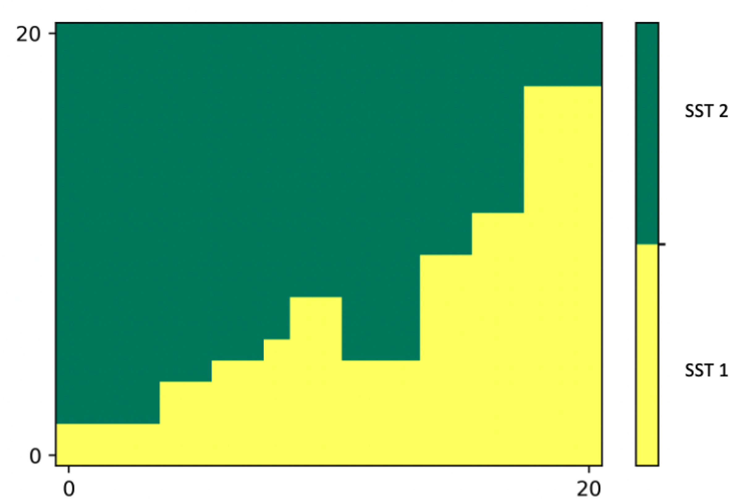
• An ideal case, in the absence of inter-channel co-registration issues, leading to the estimation of SST${}_{ret}$;
• A realistic case, introducing the co-registration error, yielding the SST${}_{coreg}$ field.

The SST gradients are then computed by means of a Sobel estimator for the SST${}_{true}$, SST${}_{ret}$ and SST${}_{coreg}$. The retrieval is simulated considering the tropical atmospheric profile of [34] and references therein. The scope of this specific exercise is, however, independent of the atmospheric composition and considering a homogeneous atmosphere over the 10 × 10 scene.

As expected, even a 10% co-registration error can generate artefacts in the SST retrieval (see the SST${}_{coreg}$ field in Figure 1c), generating a spurious feature with intermediate SST values not prescribed in the initial SST${}_{true}$ field.

The SST gradient magnitude (∇SST) is then obtained accounting for the SST gradients along the two directions. The ∇SST${}_{coreg}$ (obtained from SST${}_{coreg}$) is broader and smoother compared to the ∇SST${}_{ret}$, due to the appearance of spurious features, which are not found in the SST${}_{true}$ and SST${}_{ret}$ gradients. The co-registration is actually introducing an additional degradation on top of the inaccuracies one would get uniquely accounting for atmospheric effects. The RMSE of ∇SST${}_{ret}$ and ∇SST${}_{coreg}$ (computed using ∇SST${}_{true}$ as benchmark) indeed increases from 0.088 to 0.096 K/pixel (computed over the entire domain).

3. Methods and Data

In order to document the potential of retrieving SST gradients from single-channel TOA BTs within the Harmony mission, several aspects of the problem have to be tackled. In particular, our objectives are to achieve the following:

1.

Demonstrate that horizontal gradients of atmospheric radiatively active variables (vertical distribution of water vapor, ozone and temperature) are mostly characterized by scales of variability larger than the ones of interest for the sea surface, so that gradients in the TOA BTs can be considered to be locally determined, at a first-order approximation, by the SST ones;

2.

Quantify the attenuation of atmospheric gases (e.g., water vapor) on the magnitude of the SST gradients from TOA BT observations;

3.

Test different approaches for computing SST gradients from gridded 2D fields in order to minimize the effect of radiometric noise, whose expected extent for the Harmony mission has been presented in Table 1.

Regarding the first point, the analyses will rely on existing state-of-the-art L1.5 to L2 satellite observations (detailed below) and will also include spectral analyses based on fast Fourier transform (as in [17]) (see also Section 4.1 and Section 4.2).

The second point will be tackled via numerical simulations based on the ARTS model. In particular, we will exploit fit-for-purpose 2D synthetic SST fields and run idealized observing system simulation experiments to inter-compare a ground truth field with the estimates obtained simulating the performances of a Harmony TIR payload for different atmospheric profiles. For The ARTS model, the reader is referred to [33] as well as Appendix A of the present manuscript (see also Section 4.3).

Finally, the tests mentioned at point 3 will rely on analytical SST and SST gradient fields. We will run a specific study to determine the optimal way to numerically estimate SST gradients in the presence of radiometric noise. Similarly to point 2, the study will be carried out relying on a ground truth analytical field to assess the performances of several gradient computation techniques detailed in Appendix B (see also Section 4.4).

The satellite-derived datasets were obtained from the Sentinel 3A-SLSTR and Meteosat Second Generation 3-SEVIRI sensors, and are detailed below:

• The Sentinel-3 non-time-critical (NTC) observations distributed as L2P SST products by EUMETSAT. These products follow the Group for High Resolution Sea Surface Temperature data format specification (GHRSST, https://www.ghrsst.org/, accessed on 28 November 2022), which means they include both single-channel top-of-the-atmosphere brightness temperatures (L1) and skin SST (L2) data in the same file, together with specific L2P and user-defined SST quality flags. The quality flag is an indicator of the SST accuracy and ranges from 0 to 5: (i) 0 = missing data; (ii) 1 = cloud; (iii) 2 = worst quality, (iv) 3 = low quality; (v) 4 = acceptable quality; (vi) 5 = best quality. The L2P SST and related flags are actually those computed from dual-view data, but nadir-view SST can be recovered adding the “dual minus nadir SST difference” provided as an experimental variable in the L2P file. Here, we focused only on nadir-view data to maximize the spatial correspondence between L1 and L2 data. We selected only the highest quality flag (keeping only best quality “flag 5” data), to remove cloud-contaminated pixels, which might alter SST gradient estimates. This results in some additional artefact clouds being removed from BT/SST data. In our case study, the percentage of best quality data was estimated to be around 97%, thus guaranteeing a large availability of observations for our analyses. The L2P GHRSST data are provided in sensor coordinates. The spatial resolution of these data is around 1 km.
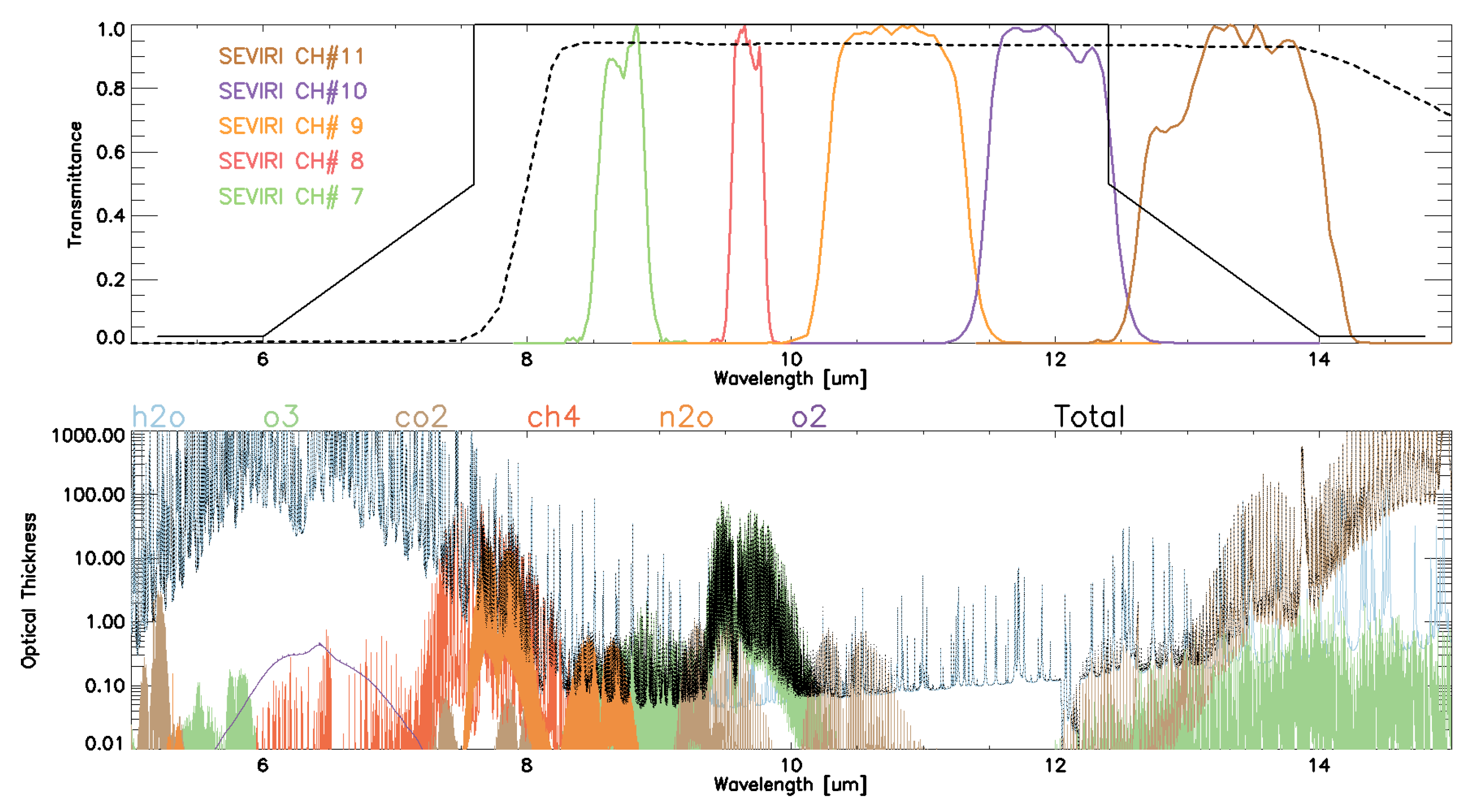
• The level 1.5 Meteosat Second Generation (MSG)-3 SEVIRI data. The data are provided as high-rate transmissions in 12 spectral channels spanning the 0.6 to 13.4 $\mathsf{\mu }$m range. The images consist of geolocated, radiometrically pre-processed data, including radiometric and geometric quality control information. The data contain TOA radiances and are expressed in $\mathrm{mW}·{\mathrm{m}}^{-2}·{\mathrm{sr}}^{-1}·{\left({\mathrm{cm}}^{-1}\right)}^{-1}$. The spatial resolution of these data is around 3 km at the subsatellite point [35]. For our purposes, we extracted information from the following IR channels: 8.7, 9.7, 10.8 and 12.0 $\mathsf{\mu }$m.

4. Results

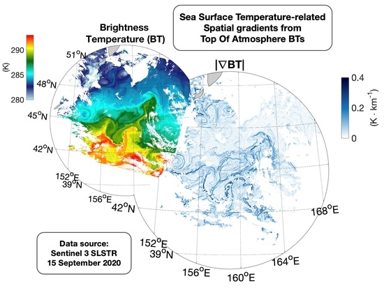
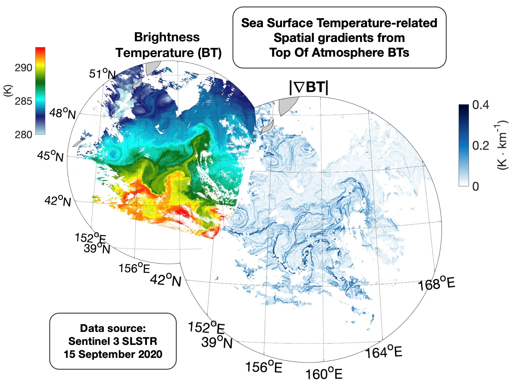
4.1. SST Gradients from L1 Observations: A Test Case

We present a test case acquired on 15 September 2020 in the North Pacific by the Sentinel 3A SLSTR sensor. The SST field (in Figure 2) is characterized by the signature of a mesoscale dipole centered at 44°N, 158°E and drifting southwestward towards the Japanese coast. The mesoscale dipole is surrounded by several submesoscale eddies and filaments with horizontal extents of the order of a few kilometers. As a consequence, the SST field exhibits a wide range of spatial gradient magnitudes, ranging from 0.05 to roughly 1 K/pixel (≃1 K/km), as depicted in Figure 3. Such a scenario will be used to test the potential of retrieving SST gradients from the Harmony PAN TOA BTs. The broad ≃ 8–12 $\mathsf{\mu }$m Harmony PAN channel will be subject to atmospheric contribution (through absorption/emission) from water vapor and ozone (9.6 $\mathsf{\mu }$m band). The ozone contribution is expected to have a low-frequency spatial variability being mostly concentrated in the stratosphere. In contrast, water vapor (WV) is expected to have higher (and somehow SST-related) spatial variability, particularly in the lower troposphere. In this exercise, we assume that the SLSTR S9 channel (centered at 12.02 $\mathsf{\mu }$m) yields observations closer to the to the ones of the future Harmony PAN. The S9 channel is indeed affected by atmospheric disturbances to a larger extent than the S8 channel (the one centered at 10.85 $\mathsf{\mu }$m) and we expect it to better mimic the atmospheric disturbances of the future PAN observations (see also [32]).

The SST gradients have been computed relying on a 3 × 3 Sobel convolution kernel [36]. The choice of the Sobel kernel will be further justified in Section 4.4 and is suitable for high-accuracy SST/BT data, such as the ones from the Sentinel 3 SLSTR sensor. Figure 3a,b, respectively, depict the SST gradient and the BT (from the S9 channel) gradient intensities, given in K/pixel (≃K/km). Based on our assumptions on the S9 channel, we then compared the gradient of the S9 channel BT (BT${}_{S9}$) with the one estimated from the SST.

Figure 3c depicts the differences between the two gradient fields, evidencing that the BT${}_{S9}$ skill in estimating the SST gradients is a function of the SST gradient itself. The low-gradient zones are well captured by both SST and BT${}_{S9}$, yielding differences of the order of ±0.05 K/pixel. However, in areas of sharp SST gradients, the BT${}_{S9}$ does not allow for the reconstruction of the full gradient intensity, exhibiting values around 0.1 to 0.2 (in some extreme cases) K/pixel weaker than the SST gradient field. These differences are very likely attributable to the water vapor (WV) effects, tending to smooth the sharpest gradients in the BT${}_{S9}$ field. This is further investigated via fast Fourier transform (FFT) spectral analysis. Focusing on the study area depicted by Figure 2 and Figure 3, we compared the power spectral density (PSD) of the SST and the difference between BT${}_{S9}$ and SST (BT${}_{S9}$-SST), the latter assumed to represent the atmospheric contribution to the TOA BT${}_{S9}$. The comparative spectral analysis, depicted in Figure 4, evidences that the SST and BT${}_{S9}$-SST spectra are superimposed for scales larger than approximately 12 km. Below this threshold, the BT${}_{S9}$-SST spectrum progressively flattens, assuming characteristics comparable with a field affected by white noise. Although this noisy behavior may result in a smoothing/smearing of the BT${}_{S9}$ largest gradients, for this case the signal associated with the atmospheric contribution exhibits a peak for scales of about 10 km, i.e., larger than the scales characterizing the strongest SST gradient structures (≃1 to 5 km).

Very interestingly, the ≃0.1 K/pixel differences in the BT${}_{S9}$-SST gradients are located exactly over the strongest SST gradient areas: their spatial distribution allows for the recognition of the gradient patterns found in Figure 3a, meaning that the position of the gradients is equally estimated by the L2 SST and L1 BT${}_{S9}$ data. This is further confirmed by Figure 3d, reporting the differences between the normalized SST and BT${}_{S9}$ gradient intensities. The normalization has been carried out accounting for maximum gradients observed in the SST and BT${}_{S9}$ maps. The resulting field is given by an overall noisy signal, where no oceanographic structure can be recognized, supporting our initial assumption on the possibility of capturing SST gradients from BT observations.

4.2. Test Case Based on SEVIRI Data

While the analysis of SLSTR is useful to simulate the spatial sampling characteristics of the Harmony TIR payload, the SLSTR S9 channel is still relatively transparent from the point of view of atmospheric effects compared to a broad 8–12 $\mathsf{\mu }$m channel. Therefore, we perform an additional investigation to mimic the atmospheric effects on the PAN channel relying on existing satellite observations. In particular, we simulate an SST gradient retrieval based on BT observations extracted from the SEVIRI MSG3 sensor (detailed in Section 3). The main assumption, here, is that a given combination of the SEVIRI channels can be seen as a proxy, in spectral terms, of the ≃8–12 $\mathsf{\mu }$m PAN channel embarked by the Harmony TIR payload.

Figure 5 (top) shows the spectral response functions (SRF) of the SEVIRI channels #7–11 as well as the preliminary ones for the Harmony PAN filter and sensor [23]. The average signal obtained combining the contributions from the SEVIRI channels #7 to 10 well approximates the signal one could get from the Harmony PAN observations. Moreover, based on [32], the SEVIRI channels 7 to 10 are mainly sensitive to the sea surface conditions, i.e., their normalized weighting functions (NWFs) are very close to 1 at 1000 hPa. Channel 8 (centered at 9.7 $\mathsf{\mu }$m) constitutes an exception: its NWF exhibits a local maximum between 20 and 30 hPa, due to the O${}_3$ absorption/emission effects (as also shown in Figure 5, bottom, green line). In this sense, the exercise based on the use of SEVIRI data enables us to quantify the relative detrimental effect of O${}_3$ on the SST gradients estimate from the PAN channel BTs. With this approach, we actually provide a worst-case scenario concerning the O${}_3$ effects. The 9.7 $\mathsf{\mu }$m channel is indeed entirely peaked over the spectral region where the O${}_3$ optical thickness exhibits a local maximum (Figure 5), preventing, e.g., the collection of the signals in the entire ≃(9 to 10 $\mathsf{\mu }$m) region, which could be achieved with the Harmony PAN channel. The results are presented in Figure 6 for the different SEVIRI channels involved in our study in a clear-sky test case for 5 August 2021 at 09:00 UTC (the clear-sky condition in correspondence of the Alboran Gyre has been double-checked with independent OSISAF SEVIRI SST data on the same date and hour, not shown).

The BTs (K) can be obtained from TOA radiances (TARs hereinafter), in mW · m${}^{-2}·$ sr${}^{-1}$· (cm${}^{-1}$)${}^{-1}$) by inverting the Planck’s law. In practice, this can be carried out using lookup tables relating radiance to brightness temperature distributed by EUMETSAT or referring to the EUMETSAT document EUM-MET-TEN-11-0569 accessible via https://www-cdn.eumetsat.int/files/2020-04/pdf_effect_rad_to_brightness.pdf, accessed on 10 December 2022. In our work, BTs were derived using the Satpy python package (https://github.com/pytroll/satpy, accessed on 10 December 2022) including tools that enabled us to read the SEVIRI L1.5 data in their native format, convert channel counts to radiance and finally obtain the BT estimates. The BT for the 10.8 $\mathsf{\mu }$m channel is sketched in Figure 6a.

The computation of the BT scene from the synthetic SEVIRI PAN channel was carried out as follows: (i) we computed the synthetic PAN monochromatic radiance averaging the radiances from the SEVIRI channels #7 to 10; (ii) we estimated the corresponding BTs inverting the Planck’s law. However, the Planck’s law can only be inverted if the spectral radiance is strictly monochromatic. This assumption fails in case of a broad 8–12 $\mathsf{\mu }$m channel, for which the effective central wavenumber (${\nu }_{eff}$) changes as a function of the observed scene. Here, the PAN channel ${\nu }_{eff}$ was obtained via a linear regression approach, as follows: (i) we accounted for a series of blackbody sources spanning a temperature range in agreement with typical SST values, i.e., from 270 to 300 K; (ii) for each blackbody source, we simulated the integrated TARs seen by each of the four SEVIRI channels (7 to 10) accounting for the SRFs obtained from https://nwp-saf.eumetsat.int, accessed on 10 December 2022; (iii) finally, averaging the integrated TARs, we searched for the wavenumber ${\nu }_{eff}$ that, applying the inverse Planck’s function, minimized the difference between the estimated BT and the temperature of the original blackbody source.

We then performed a linear regression between ${\nu }_{eff}$ and the averaged TAR (${\mathit{TAR}}_{\mathit{avg}}$) yielding the following expression:

$${\nu }_{eff}=\alpha ·TA{R}_{avg}+\beta$$

(1)

where:

• $\alpha =0.14{\mathrm{cm}}^{-2}{\mathrm{mW}}^{-1}{\mathrm{m}}^2\mathrm{sr}$;
• $\beta =971.28{\mathrm{cm}}^{-1}$.

Finally, using (1) we could successfully invert the Planck’s law and obtain the BTs associated with the SEVIRI synthetic PAN channel TARs. Computing the spatial gradients magnitude (see, e.g., Equation (A1)) from the SEVIRI BTs yielded the following scenario:

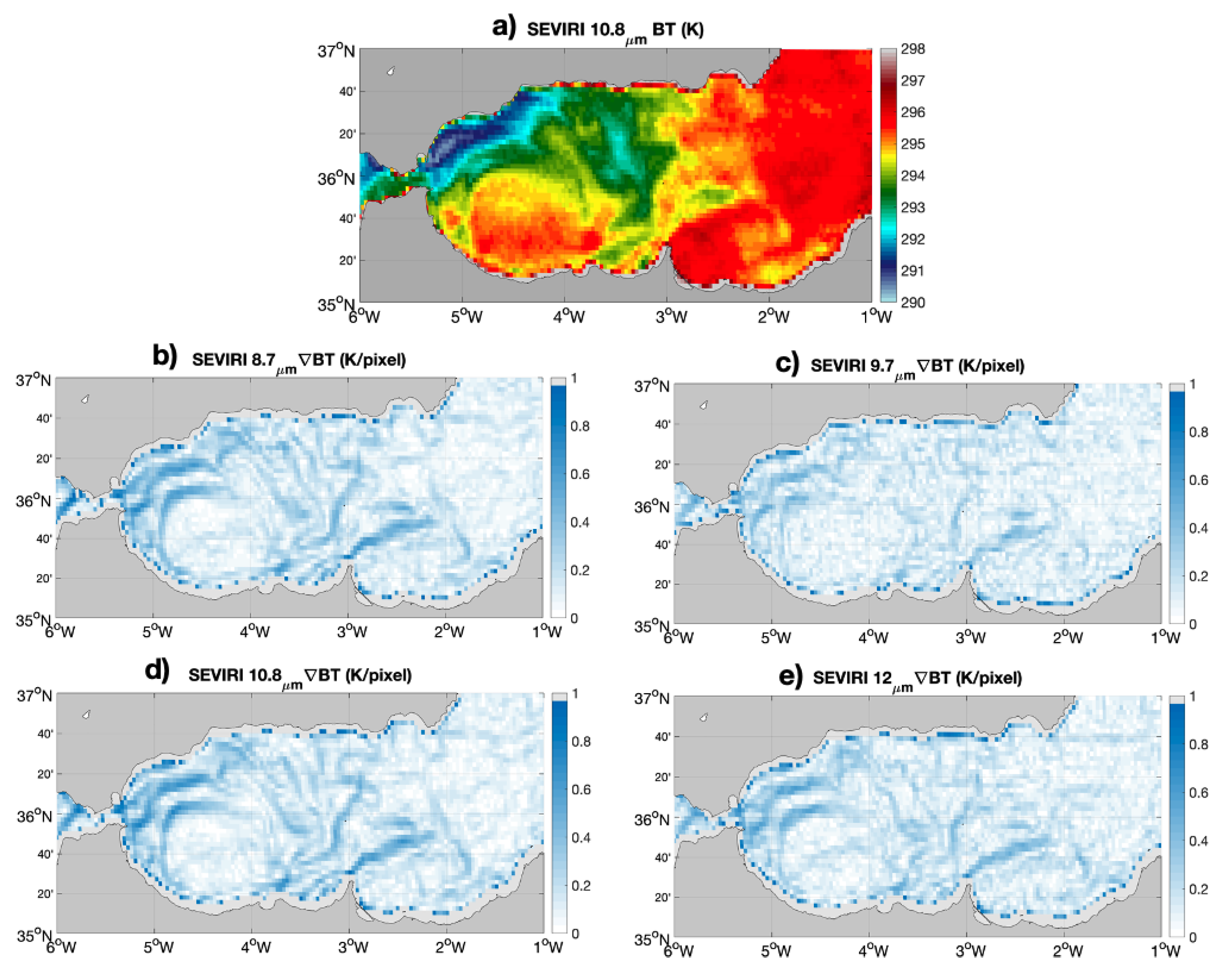
• The BT gradients shown in Figure 6b–e (given in K$·{\mathrm{pixel}}^{-1}$) differ in the description of the SST-related gradients in the selected area. Channel #9, compared to #7 and 10, exhibits the sharpest gradients. This channel is indeed characterized by the lowest NWF from 700 hPa to TOA levels and is thus chosen as a reference for the description of the sea surface [32];
• As expected, channel #8 (9.7 $\mathsf{\mu }$m) yields a highly smoothed description of the sea surface thermal conditions. The signal contains small-scale noise although still capturing some of the sharpest gradients seen by channel #9.

In the end, to support our initial assumptions, we provide a direct comparison of the BT gradients obtained from channel #9 (our reference to assess the sea surface conditions) and the averaged BTs from channels #7–10, i.e., our synthetic PAN-derived estimate.

Figure 7a,b indicate that the gradient observed from the synthetic PAN observations enables us to describe satisfactorily the main gradient features seen by the 10.8 $\mathsf{\mu }$m channel (our reference for the retrieval of the surface conditions). The SEVIRI averaged (AVG) BT gradient only looks slightly smoother than its 10.8 $\mathsf{\mu }$m counterpart. This is further quantified on a 1D transect (black dashed line in Figure 7c,d) across the edges of the Alboran Gyre, along ≃36°N. We notice that the gradient obtained from the PAN BTs (dashed line) is in fair agreement with the 12 and 8.7 $\mathsf{\mu }$m channels’ estimates and, quite interestingly, enables the retrieval of 85% of the signal intensity one would get with the 10.8 $\mathsf{\mu }$m channel (this value is representative of the mean behavior along the entire 1D transect). As discussed previously, the SEVIRI 9.7 $\mathsf{\mu }$m channel is symmetrically distributed over the spectral region where the O${}_3$ optical thickness exhibits a local maximum; therefore, these results could further improve when dealing with a wide 8–12 $\mathsf{\mu }$m window, very likely reducing the impact of the O${}_3$ radiative effects.

4.3. SST Gradients from BT Observations: Testing Water Vapor Effects

Based on the ARTS forward model described in Appendix A, we carried out a simplified observing system simulation experiment (OSSE) to confirm the preliminary results illustrated in Section 4.1. This experiment served as a preliminary estimation of the Harmony PAN channel capabilities to observe SST gradients. We compared the SST and the BT gradients for an ad hoc SST field, given by an idealized synthetic 21 × 21 pixels scene characterized by two distinct SST areas: SST${}_1$ and SST${}_2$, with SST${}_2$ = SST${}_1$ + 1K (Figure 8). Such a synthetic scene is compliant with SST fronts found in the real ocean and was used to simulate both inter-tropical and subarctic scenarios, respectively, choosing SST${}_1^{tropical}$ = 299 K and SST${}_1^{subarctic}$ =271 K and accounting for typical tropical and subarctic atmospheric compositions [34,37].

The ARTS model was then used to simulate the Harmony PAN Channel TOA radiances and derive the corresponding BTs from our SST synthetic configuration. For each scenario, the PAN BTs were simulated under the approximation of a uniform atmospheric composition throughout the 21 × 21 pixels scene, accounting for the instrument spectral characteristics and considering the fixed observation geometry discussed in Appendix A. The SST and the BT gradients were computed by means of the Sobel operator, bearing in mind that, in high-noise conditions, wider-stencils gradient operators should be accounted for (see Section 4.4). Figure 9 summarizes the key differences between the SST- and PAN-BT-based gradient estimation. In particular, for both the tropical (Figure 9a) and subarctic wintertime (Figure 9b) scenarios we show the following: (i) the SST gradient intensity (∇SST); (ii) the PAN channel BT gradient intensity (PAN ch ∇BT); (iii) the differences between the two gradient estimates (∇SST-PAN ch ∇BT). These analyses, in agreement with the results of Section 4.1, confirmed that the BT gradients can be smoothed due to water vapor absorption. The “PAN ch ∇BT” is indeed weaker for the tropical atmospheric profile, characterized by larger concentrations of water vapor. In this case, the differences between the SST- and BT-based gradient estimates (∇SST-PAN ch ∇BT) are indeed larger compared to the subarctic case (Figure 9b).

In order to be more quantitative, we also provide the bias between the TOA-PAN-BT- and SST-derived gradients (our reference case), provided in

Table 2. Bias of the TOA PAN BT gradients (expressed in K/pixel) using the SST gradients as a reference. The statistics refer to the subarctic and tropical atmospheric profiles from Garand et al. 2001.

∇ BT Gradients	Bias
Subarctic	0.11
Tropical	0.32

.

The two scenarios generate biases (computed over the areas where the gradient is larger than 0 K·pixel${}^{-1}$) that can differ by a factor of ≃3. Estimating the SST gradients from the TOA observations, using the approach presented here, enables the retrieval of 30% to 80% of the original signal depending on the local atmospheric conditions. In the perspective of retrieving the SST gradients from PAN BTs, the smoothing effects due to atmospheric contributions are a source of inaccuracies (i.e., underestimation of the intensity). The reader should, however, be aware of two strong points of such an approach, mostly related to the higher spatial resolution of the Harmony PAN channel compared to the narrow-band ones as well as the absence of co-registration effects, which were quantified introducing the present study (Section 2).

4.4. Optimizing the Gradient Numerical Scheme

The classical approach to locate satellite SST gradients is to apply derivative kernels to a given SST field. In this section, for the sake of simplicity, we will refer to SST or, more in general, fields organized on a regular grid. Examples of common kernels generally used for these purposes are the Sobel, Prewitt and Roberts, (e.g., [36,38]), as well as the one-dimensional central differences methods. A more detailed description of the gradient computation methods is provided in Appendix B. The key points to take into account when computing gradients are the accuracy in the gradient magnitude estimation, the accuracy in the gradient location and the smoothing of noise effects (see also [17]). We carried out a dedicated study to assess the relative performances of the different methodologies in an idealized context. An analytical function (aSST(x,y)) was used to mimic SST structures at the sea surface, arbitrarily simulating the case of a warm-core eddy-like feature in a 50 × 50 domain. The analytical function that mimics the SST field is expressed by (2):

$$aSST(x,y)=\xi \left(e^{-\left[{\left(\frac{x-\alpha }{\delta }\right)}^2+{\left(\frac{y-\alpha }{\delta }\right)}^2\right]}+e^{-\left[{\left(\frac{x-\beta }{ϵ}\right)}^2+{\left(\frac{y-\gamma }{\zeta }\right)}^2\right]}\right)$$

(2)

with $\xi =4,\alpha =25,\beta =20,\gamma =30,\delta =5,ϵ=4$and$\zeta =5$. The resulting aSST field is depicted by Figure 10a. The obtained shape, although generated analytically, well approximates oceanographic features, such as, e.g, an eddy undergoing deformation due to hydrodynamic instability or interactions with nearby jets or eddies [39]. The aSST field goes from 0 to 4.7, and, for convenience, can be thought of as if it was expressed in K. The corresponding gradient intensity (aGI) was also derived analytically, according to (3) and exhibits values going from 0.05 to 1 K/pixel (Figure 10b).

$$\mathrm{aGI}=|\nabla \left(\mathrm{aSST}\right)|=\sqrt{{\left[{\partial }_{\mathrm{x}}\mathrm{aSST}(\mathrm{x},\mathrm{y})\right]}^2+{\left[{\partial }_{\mathrm{y}}\mathrm{aSST}(\mathrm{x},\mathrm{y})\right]}^2}$$

(3)

Then, the aGI was compared with the numerical GIs obtained by means of the Centra, Roberts, Prewitt, Sobel and Pavel (stencil widths 5, 7, 9, 11) numerical estimators, as described in Appendix B. The exercise was carried out in both ideal conditions and in the presence of synthetic radiometric noise, obtained applying 2D random Gaussian noise with a zero mean and increasingly high standard deviation (from 0.05 to 0.25 K with discrete steps of 0.05 K) to the original aSST field. The standard deviation of the Gaussian noise must be thought of as the instrument radiometric noise and, in this sense, the choice of the 0.05–0.25 K range widely covers the expected radiometric noise of the Harmony instrument, as illustrated by Table 1. The following results were obtained:

• In ideal conditions (i.e., no noise), the finite central differences numerical scheme yields the best gradient estimates. The bias and root mean square error (RMSE) with respect to the analytical case (aGI) are, respectively, −0.0011 and 0.085 K. The wider stencil numerical schemes show comparable averaged performances but exhibit a slight degradation with respect to the central approach. Indeed, going from the Sobel to Pavel11 scheme, the bias and RMSE progressively increase, respectively, reaching −0.0065 and 0.087 K in the Pavel11 case. This behavior is mostly due to an enhanced smoothing of the gradient field for wider stencil width estimators. The Roberts estimator constitutes an exception, as it tends to misplace the gradient structure yielding inaccurate intensities (Figure 11).
• In the presence of noise, the results of the ideal scenario are reversed. The inaccuracies on the SST introduced via the Gaussian noise are highly detrimental for the gradient field. The bias and RMSE, respectively, reach 0.15 and 0.21 K for the central estimator and decrease monotonically down to 0.10 and 0.028 K for the Pavel11 case. The visual inspection of Figure 12 also enables the assessment that the Pavel11, although slightly smoothing the highest values, enables the correct representation of the gradient feature and a more refined description of the marginal area (the transition from the uniform background SST to the SST values related to our synthetic warm-core eddy). As for the previous case, the Roberts estimator constitutes an exception, exhibiting the largest bias (0.23 K), and highly degrades the gradient field as depicted by the 2D maps in Figure 12.

5. Conclusions

SST gradients are relevant features within oceanographic and atmospheric applications: their spatial patterns are the signature of ocean surface processes related to fine-scale 2D/3D oceanic motion and with impacts on the dynamics of the lower atmosphere.

More in general, describing the dynamics of SST gradient patterns (depicting frontal regions) requires a multivariate approach. As pointed out by [11] (and references therein), SST and ocean color satellite images provide valuable contributions to oceanic frontal structures studies, although they may suffer from intrinsic limitations (e.g., ocean color is a non-conservative tracer). Surface dynamics can only be understood by combining the information from tracers and direct observations of dynamical variables [40]. The Harmony candidate mission has the peculiarity of allowing co-located, simultaneous observations of SST gradients and synthetic aperture radar (SAR)-based sea surface roughness, winds and total surface currents at submesoscale resolutions, which is today achievable only by collecting information from satellite sensors mounted on different platforms. Such co-located 2D images will help understanding the coupling between the ocean and the lower atmosphere at unprecedented spatial resolutions [23].

We contributed to the Harmony mission objectives by investigating the retrieval of SST gradients from the secondary TIR payload, relying on the TOA panchromatic-derived (PAN, 8–12 $\mathsf{\mu }$m) brightness temperatures (BTs). Based on our assumptions, such an approach enables the capture of thermal gradient features at the sea surface without having to go through the SST geophysical retrieval, which may be a source of errors due to split-window algorithms (e.g., noise enhancement, inter-channel co-registration).

Analyses based on existing observations (from SLSTR on board Sentinel 3) demonstrated that the SST gradients of interest correspond to sharp features with spatial scales significantly shorter than the ones characterizing atmospheric spatial variability, making it possible to retrieve SST patterns at TOA levels. Moreover, the SLSTR S9 channel observations (a proxy of the future Harmony PAN-derived observations) enable the correct location of the main SST gradients in the TOA BTs, except for a slight degradation in the strongest features. The extent of the maximum degradation was quantified on a test case and never exceeded 0.1 to 0.2 (in few pixels) K/km. Water vapor effects were mainly deemed responsible of such slight misrepresentations.

Additional tests based on the SEVIRI imager onboard Meteosat Second Generation enabled us to further investigate the potential of the Harmony PAN channel for the retrieval of SST gradients. Extracting information from the level 1.5 native files, i.e., accounting for observations from the SEVIRI channels #7 to 10, allowed us to mimic a realistic broad 8–12 $\mathsf{\mu }$m channel. Moreover, we could also quantify the detrimental effect of atmospheric components as O${}_3$ in the SST gradients estimates obtained from TOA observations. O${}_3$ can induce a smoothing of the sharpest gradients, also introducing noise at the pixel level. Nevertheless, considering the averaged contributions of the SEVIRI channels #7 to 10 allows us to recover ≃ 85% of the SST gradient intensities observed at the sea surface.

Our investigations also took advantage of additional synthetic SST and BT scenes built by means of the Atmospheric Radiative Transfer Simulator as well as analytical functions. Such approaches made it possible to achieve the following:

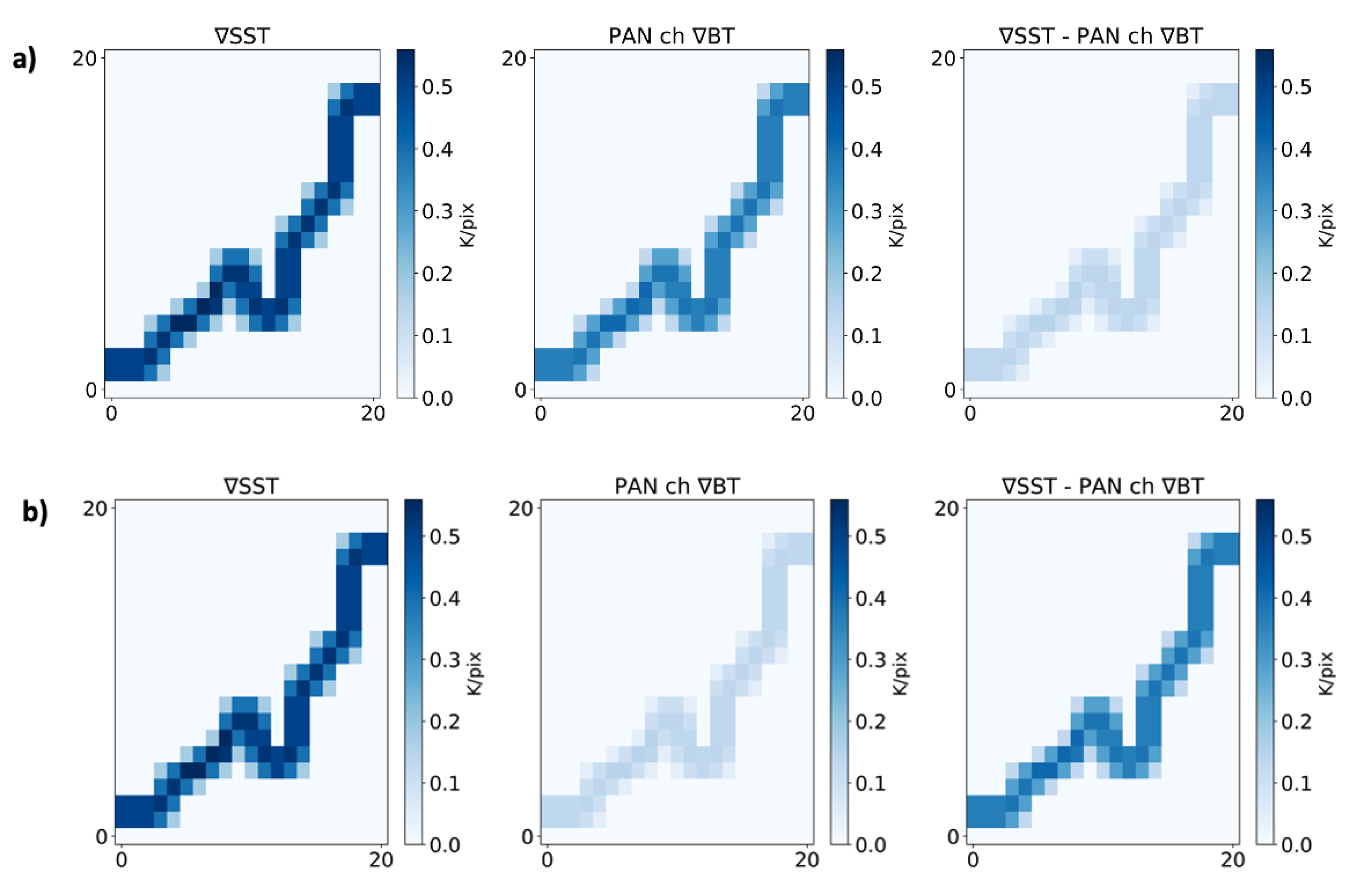
• Quantify the atmospheric effects in the space-based (TOA) PAN BT-derived SST gradients. Two extreme cases were treated, i.e., the retrieval in the presence of tropical and subarctic conditions. Very large concentrations of water vapor (typical of tropical conditions) can degrade the signal in TOA observation and allow the recovery of 30% of the gradient features found at the sea surface. However, the amount of the recovered signal can rise up to 80% if one progressively switches from tropical to typical subarctic conditions. For the specific purposes of the Harmony mission, this would favor the applicability of the proposed approach to mid-high latitude areas;
• Quantify the effect of inter-channel co-registration on the SST-based gradient retrieval, i.e., considering a co-registration issue between the TIR-1 and TIR-2 narrow-band channels by about 10% of the pixel length. This turned out to be critical for the accuracy of the gradient features extracted from SST geophysical retrievals. Not only are co-registration issues responsible for generating spurious features but they can also generate degradations of the overall gradient estimates by about 10%. This emphasizes the advantages of retrieving SST gradients from PAN-derived BTs, which enables us to get rid of any inter-channel co-registration issues;
• Assess which is the optimal numerical scheme to compute gradients from 2D BT (or SST scenes) in the presence of radiometric noise. In general, wide-stencil (i.e., at least 5 × 5) noise-robust differentiators, such as the Pavel kernels, are recommended. They indeed enable the preservation of the main gradient features even when the original 2D field is corrupted due to random noise. The chosen numerical scheme should, however, account for the number of available observations, which may vary according to the atmospheric conditions (cloud cover) or according to the distance between the study area and the coastline.

This work represents a preliminary assessment of the SST gradient observations from TOA BTs in the context of the Harmony mission. Given our analyses, the proposal to retrieve SST gradients from L1 PAN-derived observations looks promising, as it will ensure an accurate location of the main SST patterns in TOA retrievals. Additional studies are required in order to understand the extent to which the full gradient intensity can be recovered at TOA for any type of atmospheric composition/profile. This can be tackled via radiative transfer modeling, e.g., quantifying the amount of SST gradient signal that is lost in TOA estimates for a very large number of atmospheric profiles. Such an exercise could be carried out extending the analyses shown in Section 4.3 and considering the ≃4000 profiles described in [41].

In addition, advanced de-noising/filtering techniques could be implemented to further optimize the retrieval of the gradient sharpness [42,43].

References

1. Chang, Y.; Cornillon, P. A comparison of satellite-derived sea surface temperature fronts using two edge detection algorithms. Deep Sea Res. Part II Top. Stud. Oceanogr. 2015, 119, 40–47. [Google Scholar] [CrossRef] [Green Version]
2. Belkin, I.M.; Cornillon, P.C. Fronts in the world ocean’s large marine ecosystems. Ices Cm 2007, 500, 21. [Google Scholar]
3. Vazquez-Cuervo, J.; Torres, H.S.; Menemenlis, D.; Chin, T.; Armstrong, E.M. Relationship between SST gradients and upwelling off Peru and Chile: Model/satellite data analysis. Int. J. Remote Sens. 2017, 38, 6599–6622. [Google Scholar] [CrossRef]
4. Castro, S.L.; Emery, W.J.; Wick, G.A.; Tandy, W., Jr. Submesoscale sea surface temperature variability from UAV and satellite measurements. Remote Sens. 2017, 9, 1089. [Google Scholar] [CrossRef] [Green Version]
5. Messager, C.; Swart, S. Significant atmospheric boundary layer change observed above an Agulhas Current warm cored eddy. Adv. Meteorol. 2016, 2016. [Google Scholar] [CrossRef] [Green Version]
6. Warner, T.T.; Lakhtakia, M.N.; Doyle, J.D.; Pearson, R.A. Marine atmospheric boundary layer circulations forced by Gulf Stream sea surface temperature gradients. Mon. Weather. Rev. 1990, 118, 309–323. [Google Scholar] [CrossRef]
7. Barsugli, J.J.; Battisti, D.S. The basic effects of atmosphere–ocean thermal coupling on midlatitude variability. J. Atmos. Sci. 1998, 55, 477–493. [Google Scholar] [CrossRef]
8. Nilsson, J. Propagation, diffusion, and decay of SST anomalies beneath an advective atmosphere. J. Phys. Oceanogr. 2000, 30, 1505–1513. [Google Scholar] [CrossRef]
9. Woollings, T.; Hoskins, B.; Blackburn, M.; Hassell, D.; Hodges, K. Storm track sensitivity to sea surface temperature resolution in a regional atmosphere model. Clim. Dyn. 2010, 35, 341–353. [Google Scholar] [CrossRef] [Green Version]
10. Zheng, Y.; Bourassa, M.A.; Hughes, P. Influences of sea surface temperature gradients and surface roughness changes on the motion of surface oil: A simple idealized study. J. Appl. Meteorol. Climatol. 2013, 52, 1561–1575. [Google Scholar] [CrossRef]
11. Rascle, N.; Molemaker, J.; Marié, L.; Nouguier, F.; Chapron, B.; Lund, B.; Mouche, A. Intense deformation field at oceanic front inferred from directional sea surface roughness observations. Geophys. Res. Lett. 2017, 44, 5599–5608. [Google Scholar] [CrossRef] [Green Version]
12. Frenger, I.; Gruber, N.; Knutti, R.; Münnich, M. Imprint of Southern Ocean eddies on winds, clouds and rainfall. Nat. Geosci. 2013, 6, 608–612. [Google Scholar] [CrossRef]
13. Holligan, P. Biological implications of fronts on the northwest European continental shelf. Philos. Trans. R. Soc. Lond. Ser. Math. Phys. Sci. 1981, 302, 547–562. [Google Scholar]
14. Vazquez-Cuervo, J.; Gomez-Valdes, J.; Bouali, M.; Miranda, L.E.; Van der Stocken, T.; Tang, W.; Gentemann, C. Using saildrones to validate satellite-derived sea surface salinity and sea surface temperature along the California/Baja Coast. Remote Sens. 2019, 11, 1964. [Google Scholar] [CrossRef] [Green Version]
15. Wick, G.A.; Jackson, D.L.; Castro, S.L. Assessing the ability of satellite sea surface temperature analyses to resolve spatial variability—The northwest tropical Atlantic ATOMIC region. Remote Sens. Environ. 2023, 284, 113377. [Google Scholar] [CrossRef]
16. Rio, M.H.; Santoleri, R. Improved global surface currents from the merging of altimetry and sea surface temperature data. Remote Sens. Environ. 2018, 216, 770–785. [Google Scholar] [CrossRef]
17. Ciani, D.; Rio, M.H.; Nardelli, B.B.; Etienne, H.; Santoleri, R. Improving the altimeter-derived surface currents using sea surface temperature (SST) data: A sensitivity study to SST products. Remote Sens. 2020, 12, 1601. [Google Scholar] [CrossRef]
18. Isern-Fontanet, J.; García-Ladona, E.; González-Haro, C.; Turiel, A.; Rosell-Fieschi, M.; Company, J.B.; Padial, A. High-Resolution Ocean Currents from Sea Surface Temperature Observations: The Catalan Sea (Western Mediterranean). Remote Sens. 2021, 13, 3635. [Google Scholar] [CrossRef]
19. Buongiorno Nardelli, B.; Cavaliere, D.; Charles, E.; Ciani, D. Super-Resolving Ocean Dynamics from Space with Computer Vision Algorithms. Remote Sens. 2022, 14, 1159. [Google Scholar] [CrossRef]
20. Umbert, M.; Hoareau, N.; Turiel, A.; Ballabrera-Poy, J. New blending algorithm to synergize ocean variables: The case of SMOS sea surface salinity maps. Remote Sens. Environ. 2014, 146, 172–187. [Google Scholar] [CrossRef]
21. Droghei, R.; Buongiorno Nardelli, B.; Santoleri, R. A new global sea surface salinity and density dataset from multivariate observations (1993–2016). Front. Mar. Sci. 2018, 5, 84. [Google Scholar] [CrossRef] [Green Version]
22. Pearson, K.; Good, S.; Merchant, C.J.; Prigent, C.; Embury, O.; Donlon, C. Sea surface temperature in global analyses: Gains from the Copernicus Imaging Microwave Radiometer. Remote Sens. 2019, 11, 2362. [Google Scholar] [CrossRef] [Green Version]
23. ESA. Report for Assessment: Earth Explorer 10 Candidate Mission Harmony. 2020. Available online: https://atpi.eventsair.com/ucm-2022/ucm-doc (accessed on 13 August 2022).
24. López-Dekker, P.; Biggs, J.; Chapron, B.; Hooper, A.; Kääb, A.; Masina, S.; Mouginot, J.; Buongiorno Nardelli, B.; Pasquero, C.; Prats-Iraola, P.; et al. The Harmony mission: End of phase-0 science overview. In Proceedings of the 2021 IEEE International Geoscience and Remote Sensing Symposium IGARSS, Brussels, Belgium, 11–16 July 2021; pp. 7752–7755. [Google Scholar]
25. ESA. Report for Mission Selection: Earth Explorer 10 Candidate Mission Harmony. 2022. Available online: https://www.esa.int/Applications/Observing_the_Earth/FutureEO/Preparing_for_tomorrow/Scientific_and_technical_mission_documents (accessed on 26 June 2022).
26. Coppo, P.; Brandani, F.; Faraci, M.; Sarti, F.; Dami, M.; Chiarantini, L.; Ponticelli, B.; Giunti, L.; Fossati, E.; Cosi, M. Leonardo spaceborne infrared payloads for Earth observation: SLSTRs for Copernicus Sentinel 3 and PRISMA hyperspectral camera for PRISMA satellite. Appl. Opt. 2020, 59, 6888–6901. [Google Scholar] [CrossRef] [PubMed]
27. Inoue, T. On the temperature and effective emissivity determination of semi-transparent cirrus clouds by bi-spectral measurements in the 10μm window region. J. Meteorol. Soc. Jpn. Ser. II 1985, 63, 88–99. [Google Scholar] [CrossRef] [Green Version]
28. Sassen, K.; Grund, C.J.; Spinhirne, J.D.; Hardesty, M.M.; Alvarez, J.M. The 27–28 October 1986 FIRE IFO cirrus case study: A five lidar overview of cloud structure and evolution. Mon. Weather. Rev. 1990, 118, 2288–2312. [Google Scholar] [CrossRef]
29. Montanaro, M.; Levy, R.; Markham, B. On-orbit radiometric performance of the Landsat 8 Thermal Infrared Sensor. Remote Sens. 2014, 6, 11753–11769. [Google Scholar] [CrossRef] [Green Version]
30. Scalione, T.; De Luccia, F.; Cymerman, J.; Johnson, E.; McCarthy, J.K.; Olejniczak, D. VIIRS initial performance verification. Subassembly, early integration and ambient phase I testing of EDU. In Proceedings of the 2005 IEEE International Geoscience and Remote Sensing Symposium, Seoul, Republic of Korea, 25–29 July 2005; Volume 1, p. 4. [Google Scholar]
31. Francois, C.; Brisson, A.; Le Borgne, P.; Marsouin, A. Definition of a radiosounding database for sea surface brightness temperature simulations: Application to sea surface temperature retrieval algorithm determination. Remote Sens. Environ. 2002, 81, 309–326. [Google Scholar] [CrossRef]
32. Schmetz, J.; Pili, P.; Tjemkes, S.; Just, D.; Kerkmann, J.; Rota, S.; Ratier, A. An introduction to Meteosat second generation (MSG). Bull. Am. Meteorol. Soc. 2002, 83, 977–992. [Google Scholar] [CrossRef]
33. Eriksson, P.; Buehler, S.; Davis, C.; Emde, C.; Lemke, O. ARTS, the atmospheric radiative transfer simulator, version 2. J. Quant. Spectrosc. Radiat. Transf. 2011, 112, 1551–1558. [Google Scholar] [CrossRef] [Green Version]
34. Garand, L.; Turner, D.; Larocque, M.; Bates, J.; Boukabara, S.; Brunel, P.; Chevallier, F.; Deblonde, G.; Engelen, R.; Hollingshead, M.; et al. Radiance and Jacobian intercomparison of radiative transfer models applied to HIRS and AMSU channels. J. Geophys. Res. Atmos. 2001, 106, 24017–24031. [Google Scholar] [CrossRef] [Green Version]
35. Schmid, J. The SEVIRI instrument. In Proceedings of the 2000 EUMETSAT Meteorological Satellite Data User’s Conference, Bologna, Italy, 29 May–2 June 2000; Volume 29, pp. 13–32. [Google Scholar]
36. Jin-Yu, Z.; Yan, C.; Xian-Xiang, H. Edge detection of images based on improved Sobel operator and genetic algorithms. In Proceedings of the 2009 International Conference on Image Analysis and Signal Processing, Linhai, China, 11–12 April 2009. [Google Scholar]
37. Anderson, G.P.; Clough, S.A.; Kneizys, F.; Chetwynd, J.H.; Shettle, E.P. AFGL Atmospheric Constituent Profiles (0.120 km); Technical Report; Air Force Geophysics Lab Hanscom AFB MA; Defense Technical Information Center: Fort Belvoir, VA, USA, 1986. [Google Scholar]
38. Rafati, M.; Arabfard, M.; Rafati-Rahimzadeh, M. Comparison of different edge detections and noise reduction on ultrasound images of carotid and brachial arteries using a speckle reducing anisotropic diffusion filter. Iran. Red Crescent Med. J. 2014, 16, e14658. [Google Scholar] [CrossRef] [PubMed] [Green Version]
39. Carton, X. Hydrodynamical modeling of oceanic vortices. Surv. Geophys. 2001, 22, 179–263. [Google Scholar] [CrossRef]
40. Chapron, B.; Collard, F.; Ardhuin, F. Direct measurements of ocean surface velocity from space: Interpretation and validation. J. Geophys. Res. Ocean. 2005, 110. [Google Scholar] [CrossRef]
41. Eresmaa, R.; McNally, A.P. Diverse profile datasets from the ECMWF 137-level short-range forecasts. NWPSAF-EC-TR-017 2014, 10, 4476–8963. [Google Scholar]
42. Li, X.; Xiao, J.; Zhou, Y.; Ye, Y.; Lv, N.; Wang, X.; Wang, S.; Gao, S. Detail retaining convolutional neural network for image denoising. J. Vis. Commun. Image Represent. 2020, 71, 102774. [Google Scholar] [CrossRef]
43. Tian, C.; Xu, Y.; Li, Z.; Zuo, W.; Fei, L.; Liu, H. Attention-guided CNN for image denoising. Neural Netw. 2020, 124, 117–129. [Google Scholar] [CrossRef]
44. Davies, E.R. Machine Vision: Theory, Algorithms, Practicalities; Elsevier: Amsterdam, The Netherlands, 2004. [Google Scholar]
Figure 1. (a) Reference synthetic SST field (SST t r u e ); (b) SST field retrieved via the NL split-window algorithm of [31]; (c) SST retrieved via the NL split-window algorithm considering the co-registration on the Harmony TIR-1 channel (SST c o r e g ). Gradient magnitude of the (d) SST t r u e ; (e) SST r e t field; (f) SST c o r e g field.
Remotesensing 15 01163 g001
Figure 2. Sea surface temperature scene acquired by the S3 SLSTR sensor in the North Pacific acquired on 15 September 2020, 09:00 UTC. White areas stand for SST with quality level lower than 5.
Remotesensing 15 01163 g002
Figure 3. Maps of (a) SST gradient intensity (GI), (b) S9 channel-derived BT (BT S 9 ) GI, (c) difference between BT S 9 and SST GIs, (d) difference between the normalized BTS9 and SST GIs. In panels (a,b), the colorscale is limited to 0.45 K/pixel with the aim of visually emphasizing the gradient features.
Remotesensing 15 01163 g003
Figure 4. Power spectral density of the BT S 9 -SST (blue) and SST (red) fields computed over the area depicted in Figure 2 and Figure 3. The relative positions of the 12 km and 5 km scales are given by the green dashed lines.
Remotesensing 15 01163 g004
Figure 5. (Top) Black continuous/dotted lines: preliminary spectral response function of the Harmony panchromatic channel/sensor. Colored lines refer to the SEVIRI channels: green (channel 7), 8.7 μ m; red (channel 8), 9.7 μ m; orange (channel 9), 10.8 μ m; purple (channel 10), 12.0 μ m; brown (channel 11), 13.4 μ m. (Bottom) Example of optical thicknesses of the main atmospheric absorbing gases in the 5–15 μ m range (http://eodg.atm.ox.ac.uk/ATLAS/zenith-absorption, accessed on 26 June 2022).
Remotesensing 15 01163 g005
Figure 6. (a) TOA radiances for SEVIRI channel 9. (be) Sobel spatial gradients of the TOA radiances for channels 7 to 11. The fields refer to 5 August 2021 at 09:00 UTC.
Remotesensing 15 01163 g006
Figure 7. (a) Sobel spatial gradients of BT for SEVIRI channel #9. (b) Sobel spatial gradients of BT from the SEVIRI simulated PAN. (c) Zoom over the Alboran Gyre area, depicting in detail the 1D transect for the extraction of gradient magnitudes at 36°N. (d) Gradient magnitudes at 36°N: blue, red, yellow, green and dashed black lines, respectively, refer to gradient magnitudes seen by the 8.7, 9.7, 10.8, 12.0 μ m and synthetic PAN channels.
Remotesensing 15 01163 g007
Figure 8. Synthetic SST field for the OSSE on the Harmony-derived SST gradients. SST 2 = SST 1 + 1K.
Remotesensing 15 01163 g008
Figure 9. SST- and PAN-BT-derived gradient ( K · p i x e l 1 ) comparison for subarctic winter (a) and tropical (b) cases. From left to right: SST gradient, BT gradient and the difference of the two fields.
Remotesensing 15 01163 g009
Figure 10. (a) Analytical SST field (aSST, in K); (b) analytical SST gradient intensity (aGI, in K/pixel).
Remotesensing 15 01163 g010
Figure 11. (a) Gradient intensities computed numerically using central, Roberts, Sobel, Prewitt and Pavel 5 to 11 schemes. (b) RMSE (blue) and bias (orange) of the numerically computed gradient with respect to the analytical ground truth value calculated from the noise-free temperature field using Equation (3), units are in K. The analyses refer to the ideal case: absence of noise.
Remotesensing 15 01163 g011
Figure 12. (a) Gradient intensities computed numerically using central, Roberts, Sobel, Prewitt and Pavel5 to 11 schemes. (b) RMSE (blue) and bias (orange) of the numerically computed gradient with respect to the analytical ground truth value calculated from the noise-free temperature field using Equation (3), units are in K. The analyses refer to an aSST field with addition of Gaussian noise with a zero mean and standard deviation of 0.15 K.
Remotesensing 15 01163 g012