Multiscale Analysis of Reflected Radiation on Lunar Surface Region Based on MRRT Model

Abstract

The moon has stable luminosity. Radiometric calibration on the lunar region is a good step in the right direction with the expansion of instrument observation capabilities. The uneven composition and terrain types of the lunar surface make it possible for inaccuracies in albedo calculation from coarse-scale data if the within-pixel topology is overlooked. The expression between the region’s bidirectional reflectance factor (BRF) and the actual microtopography reflectance was established by the multiple reflections of radiation between terrains (MRRT) model. This research studied the radiation properties on the lunar surface region at various spatial resolutions (scales) based on the MRRT model. To determine the ideal scale of microtopography to be built, the scale-effect evaluation factor of albedo is established, and the scale-effect function is fitted. Experiments demonstrate that a microtopography with a spatial resolution of 60 m to 120 m, with 80 m being the most suitable scale, can be constructed for an area having (6000 × 6000) m². This research adds to the MRRT model’s applicability analysis in multiscale DEM modeling, helps choose and build a radiation calibration field on the lunar surface, and lays the groundwork for employing the area of the lunar surface for radiation calibration.

1. Introduction

The moon has stable luminosity ideal for a calibration source. By determining the empirical parameters of the functional expression of the lunar equivalent disc reflectance by fitting the data observed by the varied illumination observation geometries, the Robotic Lunar Observatory (ROLO) is constructed to use the moon for radiometric calibration [1]. The ROLO model, which has an uncertainty of 5–10%, is currently the most accurate lunar radiation model available [2]. Several initiatives have been made to make the model the sole recognized benchmark for lunar calibration [3]. The needed calibration accuracy has, however, exceeded the upper bounds of this model’s calibration accuracy. In contrast, radiometric calibration based on the lunar surface region is an appropriate development direction with the expansion of the observational capabilities of remote sensing devices [4].

The link between remote sensing images with various spatial resolutions, however, is not simply average, but rather connected to the surface conditions and the characteristics of the target (geo) parameters due to the spatial heterogeneity of the topographic surface [5]. Target isotropy can in fact only be expressed to a limited extent due to the scale effect; for example, a target with uniform radiation properties at a small scale is not always isotropic at a large scale [6]. The majority of research demonstrates that the scale effect is the main factor contributing to albedo estimation uncertainty, and that topography’s influence on remote sensing data is spatially scale-dependent [7,8,9]. The moon is not a perfect Lambert body, and the terrain types and composition of the lunar surface are heterogeneous [10,11]. It is obvious that the luminance of the lunar surface changes with topography and is connected to albedo [11]. Based on statistical approaches, Yokota et al. [12] identified three albedo groups on the surface of the moon, and by using novel correction parameters of the high albedo group, they produced a 1${}^{\circ }$ mesh global lunar reflectance map cube with 160 bands (wavelengths: 512–1652 nm). Based on the percentage of FeO concentration, Wu et al. [13] classified the lunar surface into four types of terrain.

However, the influence of macrotopography, particularly the multiple reflection effects between terrains, on the photometric properties of the lunar surface is rarely taken into account or computed. Wu et al. [14] noted that the Interference Imaging Spectrometer (IIM) model has relatively large model errors in high-latitudes and edge regions. Topographic information must be taken into account when a local portion of the lunar surface is used for calibration in order to examine the problem of rim modeling and improve the precision of irradiance simulation [14]. In addition, Zeng et al. [10] recommended that while assessing the impact of heterogeneous correction factors on lunar irradiance, it should be sought to take into consideration the numerous radiation reflections induced by terrain. To create a topographic correction model appropriate for the lunar surface, Chen et al. [15] simplified the Sandmeier model; nonetheless, the reflected radiation from the nearby topography is actually used instead by the average reflectivity of the nearby pixels. The accuracy of the mean reflectance obtained by using the surrounding pixels cannot be guaranteed due to the complexity of the terrain [16,17]. The Hapke model [18] is a radiation transmission model with a clear physical meaning; however, it has many factors with intricate mathematical relationships and challenges in solving them, which are frequently simplified to a variety of models to use without taking topographic effects into account [19]. Furthermore, although Hapke came up with the formula for macroscopic roughness, it made the often-untrue assumption that the slope of the terrain would follow a normal distribution [20]. Liu [4] developed the multiple reflections of radiation between terrains (MRRT) model based on Proy’s single reflection of the adjacent terrain irradiance formula [21]. Liu [4] then demonstrated that, despite the lunar surface region having almost no atmospheric effect, the multiple reflections of radiation between macroscopic terrains are not insignificant. However, a thorough analysis of the MRRT model’s radiation reflection properties at various scales has not been done.

Based on the MRRT model, the radiation properties on the lunar surface region at various spatial resolutions (scales) are discussed in this work. To show the viability of the MRRT model for the multiscale investigation of topographic radiation characteristics, it is compared to the Hapke model. The scale-effect evaluation factor is then established in order to normalize the albedo inaccuracy at various sizes. The scale-effect function is fitted to determine the ideal ratio between the microtopography and the overall observation area in the MRRT model based on the scale-effect evaluation factor. The radiation calibration field is therefore established on the lunar surface using DEM data with the appropriate spatial resolution. The experimental findings demonstrate that there exists a critical point of scale wherein an increase in DEM data has little impact on the calculation of actual albedo, even though in an ideal world more DEM grid data would improve the calculation results. For a region with a size of (6000 × 6000) m${}^2$, it is permissible to create a microtopography with a spatial resolution ranging from 60 m to 120 m and to perform albedo calculations; however, the spatial resolution of 80 m is the scale that is most suitable. This study adds to the MRRT model’s applicability analysis in multiscale DEMs modeling and lays the groundwork for using the lunar surface as a radiation calibration field by helping to choose and build a radiation calibration field there.

2. Methodology

Using information from the Lunar Orbiter Laser Altimeter (LOLA), the topography of the lunar surface region is identified in this study. DEM data are created at various scales to assess the scale influence on topographic radiation properties. The general process is as follows: the creation of multiscale digital elevation models (DEMs), MRRT model-based albedo derivation, specification of scale-effect evaluation factor, comparison of albedo at various scales, and curve fitting of scale effect function. The analytical process’s specifics are provided below.

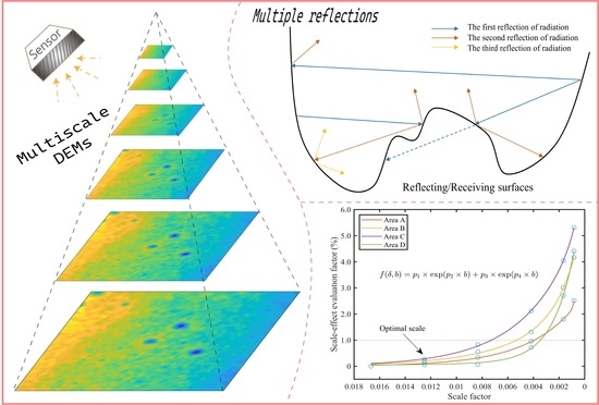
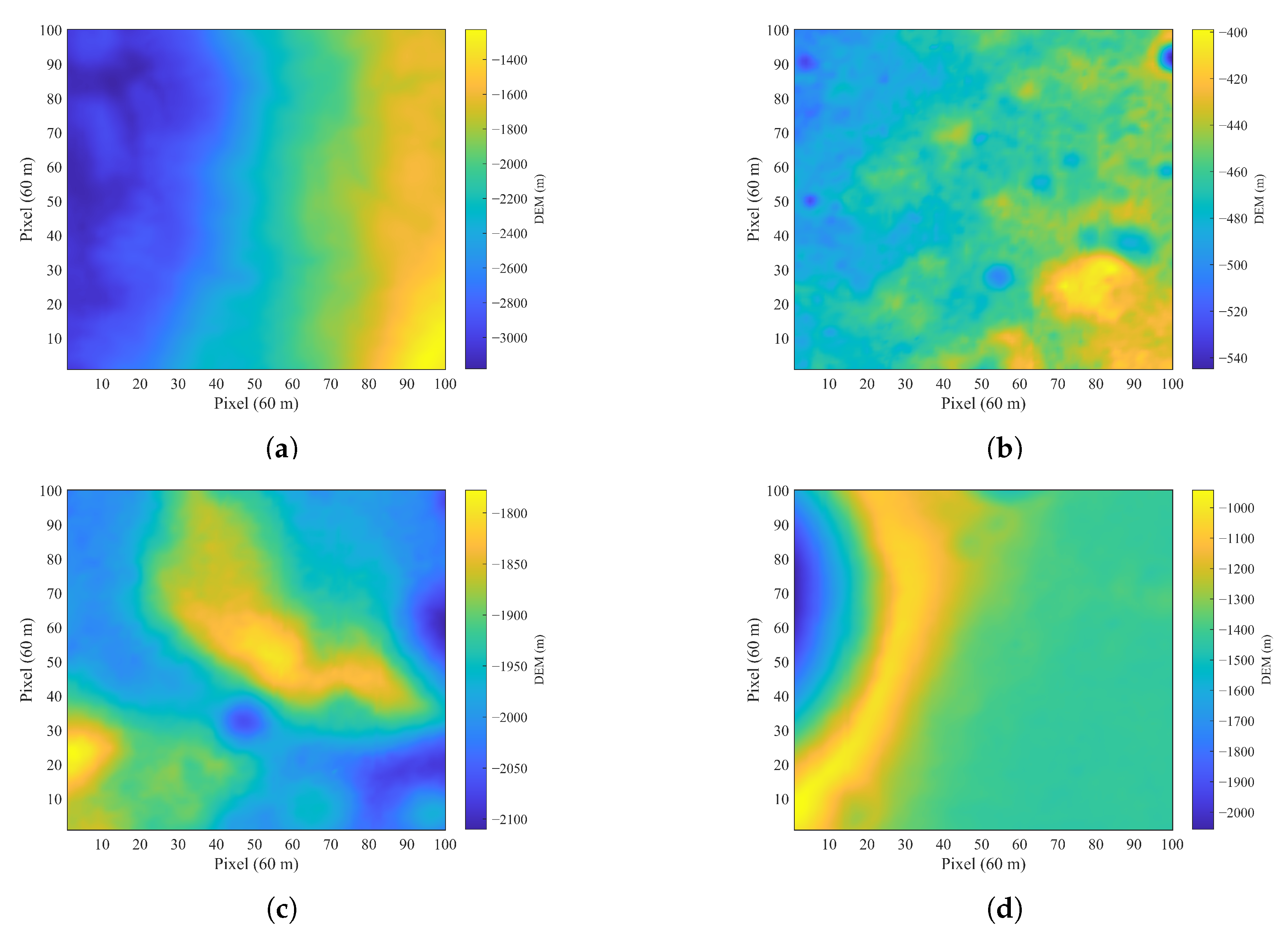
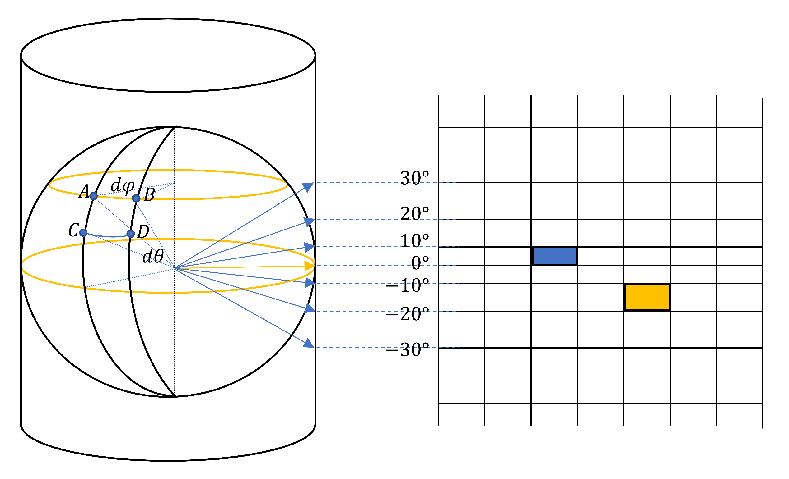
2.1. Creation of Multiscale Digital Elevation Models

Barker et al. [22] merged the DEMs from the SELENE terrain camera (TC) and LOLA DEMs to create SLDEM2015 (http://imbrium.mit.edu/DATA/SLDEM2015/, accessed on 24 January 2022), a near-global DEM with greater geodetic accuracy. The spatial resolution of the dataset used in this work was 512 pixels per degree (about 60 m per pixel at the equator). The multiscale topography was created using LOLA data with resolutions of 60, 80, 120, 240, 600, and 1200 m per pixel. For information on the selected lunar surface regions, see Appendix A.1. The function “imresize” in Matlab was used to implement the downsampling of LOLA data. The zoom factor was set to 1, 0.75, 0.5, 0.25, 0.1, and 0.05, and the interpolation method was “bicubic”. As a result, the created grids for the DEMs had the following sizes: $100\times 100$, $75\times 75$, $50\times 50$, $25\times 25$, $10\times 10$, and $5\times 5$. Using the Chang’e-3 landing region, as an illustration, Figure 1 displays the multi-scale DEM produced.

Figure 1 demonstrates how image loss texture details increase as the spatial resolution of the terrain decreases. The entropy of each DEM at various scales is determined using Equation (1) [23] in order to quantify the textures’ finer features.

$$e=-\sum _{i=0}^{L-1}p\left(z_i\right)log2p\left(z_i\right)$$

(1)

where L is the total number of grey levels, $p\left(z_i\right)$ is the frequency of each grey level, and z is a random variable indicating the DEM’s grey levels. Entropy increases with DEM variance; if DEM values are uniform across the lunar surface, entropy is equal to zero [10].

Table 1. The DEMs’ entropy at six distinct scales.

Size (Pixels)	$100\times 100$	$75\times 75$	$50\times 50$	$25\times 25$	$10\times 10$	$5\times 5$
Entropy	4.637891	4.218428	4.195238	3.138591	2.798955	1.498689

provides the entropy of the DEMs at six distinct scales. The outcome demonstrates that at the Chang’e-3 landing zone, the entropy reduces from 4.637891 to 1.498689 with a loss in topographic spatial resolution, suggesting that the reduction of the terrain’s spatial resolution will “blur” the landscape’s relief and make the topography “look” flat.

The topographic slope’s averages and standard deviations at six distinct scales are displayed in Figure 2.

2.2. MRRT Model-Based Albedo Derivation

The total incoming reflectance or radiance is strongly topographically dependent due to the effects of rough terrain, which frequently affect lighting and viewing geometry, produce a relief shadow, observation masking, and multiple scattering [8]. The neighboring terrain irradiance formula proposed by Proy, which took into account the single reflected radiation between terrains, was used by Liu [4] to derive the second-order to the nth-order reflections of radiation between terrains; the relationship between the bidirectional reflectance factor (BRF) of the observed pixel and the genuine microtopography reflectance is established, as shown in Equation (11). The following is a simple explanation of how the MRRT model was derived.

The slope surfaces with varying reflectance are thought to be Lambertian. $P_j$ is the jth slope that can reflect M, where M is the received slope. The total irradiance that slope M got from all “visible” $P_j$ can then be expressed as follows [21]:

$$E_M=\sum _j{\rho }_{P_j}\frac{E_{P_j}cos{T}_{M}cos{T}_{P_j}d{S}_{P_j}}{\pi r_{M{P}_j}^2}$$

(2)

where $d{S}_{P_j}$, $E_{P_j}$ and ${\rho }_{P_j}$ are the area, the irradiance and the reflectance of pixel $P_j$; $T_M$ and $T_{P_j}$ are the angles formed by the line $M{P}_j$ and the slope’s normal; and $r_{M{P}_j}$ is the distance between M and $P_j$.

In the event that ${\rho }_M{E}_M$ does not equal 0, ${\rho }_M{E}_M$ will continue to take part in the subsequent reflection along with other slopes. Following each radiation reflection, the incident irradiance on each microarea surface can be calculated as follows:

$$\begin{array}{cc}\hfill E_M\left(1\right)& =E_{(sun\to M)},E_{P_j}\left(1\right)=E_{(sun\to P_j)}\hfill \end{array}$$

(3a)

$$\begin{array}{cc}\hfill E_M\left(n\right)& =\sum _j{\rho }_{P_j}\frac{cos{T}_{M}cos{T}_{P_j}d{S}_{P_j}}{\pi r_{M{P}_j}^2}·E_{P_j}(n-1)\hfill \end{array}$$

(3b)

where $E_M\left(n\right)$ is the total incident irradiance that the slope’s surface M has received for the nth time. The radiation transmission from the sun to the slope M is represented by the subscript “$sun\to M$”.

Let

$${\mathsf{\Gamma }}_{M{P}_j}=\frac{cos{T}_{M}cos{T}_{P_j}d{S}_{P_j}}{\pi r_{M{P}_j}^2}$$

(4)

Hence ${\mathsf{\Gamma }}_{M{P}_j}$ can be thought of as the visible radiation factor of M. Evidently, ${\mathsf{\Gamma }}_{M{P}_j}$ does not change depending on the quantity of reflections.

In order to create many microareas with various slope, aspect, and elevation values, the target terrain is divided into equally spaced intervals. Lambert’s reflection is taken into account and the microarea reflectance is assumed to be $\rho$. Equations (5)–(8) demonstrate how matrix $T_n$ stores the incident irradiance on the surface of each DEM pixel of the nth-order.

$$T_1=E_0=\left[\begin{array}{cccc}{E}_{11}& E_{12}& \cdots & E_{1c}\\ E_{21}& E_{22}& \cdots & E_{2c}\\ ⋮& ⋮& \ddots & ⋮\\ E_{r1}& E_{r2}& \cdots & E_{rc}\end{array}\right],n=1$$

(5)

$$T_2=\left[\begin{array}{cccc}\rho ·\sum (T_1\odot {\mathsf{\Gamma }}_{(1,1)})& \rho ·\sum (T_1\odot {\mathsf{\Gamma }}_{(1,2)})& \cdots & \rho ·\sum (T_1\odot {\mathsf{\Gamma }}_{(1,c)})\\ \rho ·\sum (T_1\odot {\mathsf{\Gamma }}_{(2,1)})& \rho ·\sum (T_1\odot {\mathsf{\Gamma }}_{(2,2)})& \cdots & \rho ·\sum (T_1\odot {\mathsf{\Gamma }}_{(2,c)})\\ ⋮& ⋮& \ddots & ⋮\\ \rho ·\sum (T_1\odot {\mathsf{\Gamma }}_{(r,1)})& \rho ·\sum (T_1\odot {\mathsf{\Gamma }}_{(r,2)})& \cdots & \rho ·\sum (T_1\odot {\mathsf{\Gamma }}_{(r,c)})\end{array}\right],n=2$$

(6)

$$T_3=\left[\begin{array}{cccc}\rho ·\sum (T_2\odot {\mathsf{\Gamma }}_{(1,1)})& \rho ·\sum (T_2\odot {\mathsf{\Gamma }}_{(1,2)})& \cdots & \rho ·\sum (T_2\odot {\mathsf{\Gamma }}_{(1,c)})\\ \rho ·\sum (T_2\odot {\mathsf{\Gamma }}_{(2,1)})& \rho ·\sum (T_2\odot {\mathsf{\Gamma }}_{(2,2)})& \cdots & \rho ·\sum (T_2\odot {\mathsf{\Gamma }}_{(2,c)})\\ ⋮& ⋮& \ddots & ⋮\\ \rho ·\sum (T_2\odot {\mathsf{\Gamma }}_{(r,1)})& \rho ·\sum (T_2\odot {\mathsf{\Gamma }}_{(r,2)})& \cdots & \rho ·\sum (T_2\odot {\mathsf{\Gamma }}_{(r,c)})\end{array}\right],n=3$$

(7)

Therefore,

$$T_n=\rho ·\left[\begin{array}{cccc}\sum (T_{n-1}\odot {\mathsf{\Gamma }}_{(1,1)})& \sum (T_{n-1}\odot {\mathsf{\Gamma }}_{(1,2)})& \cdots & \sum (T_{n-1}\odot {\mathsf{\Gamma }}_{(1,c)})\\ \sum (T_{n-1}\odot {\mathsf{\Gamma }}_{(2,1)})& \sum (T_{n-1}\odot {\mathsf{\Gamma }}_{(2,2)})& \cdots & \sum (T_{n-1}\odot {\mathsf{\Gamma }}_{(2,c)})\\ ⋮& ⋮& \ddots & ⋮\\ \sum (T_{n-1}\odot {\mathsf{\Gamma }}_{(r,1)})& \sum (T_{n-1}\odot {\mathsf{\Gamma }}_{(r,2)})& \cdots & \sum (T_{n-1}\odot {\mathsf{\Gamma }}_{(r,c)})\end{array}\right],n>1$$

(8)

where the matrix $E_0$ represents the solar direct incident irradiance. Grid points in row r and column c receive actual sun incident irradiance $E_{rc}$, and the visible radiation factor between this location pixel and other pixels is represented by ${\mathsf{\Gamma }}_{(r,c)}$. The multiplication of each element in the corresponding place of the matrices $T_{n-1}$ and $\mathsf{\Gamma }(r,c)$ yields a matrix of the same size, which is represented by $T_{n-1}\odot {\mathsf{\Gamma }}_{(r,c)}$. The expression $\sum (T_{n-1}\odot {\mathsf{\Gamma }}_{(r,c)})$ specifies the addition of each component of the final matrix. The detailed calculation steps of $E_0$ and ${\mathsf{\Gamma }}_{(r,c)}$ can be gained from the literature [4].

Throughout numerous radiative reflections, each element in $T_n$ steadily approaches 0. The ultimate total reflection of the DEM image to the sky, $L_{ref}$, can then be stated as follows:

$$L_{ref}=\frac{\rho }{\pi }(T_1+T_2+T_3\cdots +T_n)$$

(9)

Assess the impact of microtopography on a single observation pixel for remote sensing. Let $T_n=\rho ·D_{n-1},(n>1)$. $D_{n-1}$ represents the ($n-1$)th reflection effect between terrains. When $n=1$, $D_0=T_1=E_0$. $L_{ref}$ can be written as follows:

$$L_{ref}=\frac{\rho }{\pi }(T_1+T_2+T_3\cdots +T_n)=\frac{\rho D_0+{\rho }^2(D_1+D_2+\cdots +D_{n-1})}{\pi }$$

(10)

Equation (11) then displays the bidirectional reflectance factor (BRF) for the observation region of a single pixel.

$$BRF({\theta }_0,{\varphi }_0,{\theta }_v,{\phi }_v)=\frac{\pi L_v({\theta }_0,{\varphi }_0,{\theta }_v,{\phi }_v)}{E_{sun}cos\left({\theta }_0\right)}=\frac{\rho D_0+{\rho }^2(D_1+D_2+\cdots +D_{n-1})}{E_{sun}cos\left({\theta }_0\right)}\odot B_v$$

(11)

where the angles of the sun’s zenith, azimuth, observation zenith, and observation azimuth are denoted by the symbols ${\theta }_0$, ${\varphi }_0$, ${\theta }_v$, and ${\phi }_v$, respectively. With a calculation akin to that of $E_0$, $B_v$ is the binary visibility matrix in the direction of observation, and $E_{sun}$ is the direct solar irradiation. There is only one reflection from the terrain surface when the topography is perfectly horizontal. Therefore, $D_0=E_{sun}cos\left({\theta }_0\right)$, $B_v=1$, and $BRF={\rho }_v$.

Equation (11) demonstrates how the topography of the microarea has an impact on the BRF (i.e., apparent reflectance) of remote sensing pixels observed in low spatial resolution. It is possible to calculate apparent albedo, also known as topographic-effect albedo, by integrating the apparent reflectance across all sensor view angles [8], i.e.,

$$Albedo=\frac{1}{\pi }{\int }_0^{2\pi }{\int }_0^{\pi /2}BRF({\theta }_0,{\varphi }_0,{\theta }_v,{\phi }_v)cos{\theta }_{v}sin{\theta }_{v}d{\theta }_{v}d{\phi }_v$$

(12)

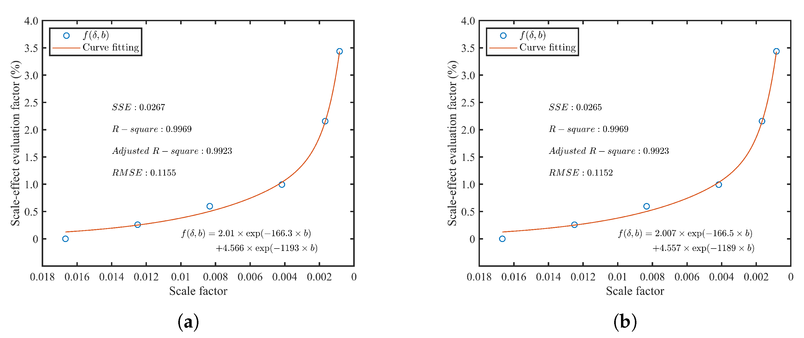
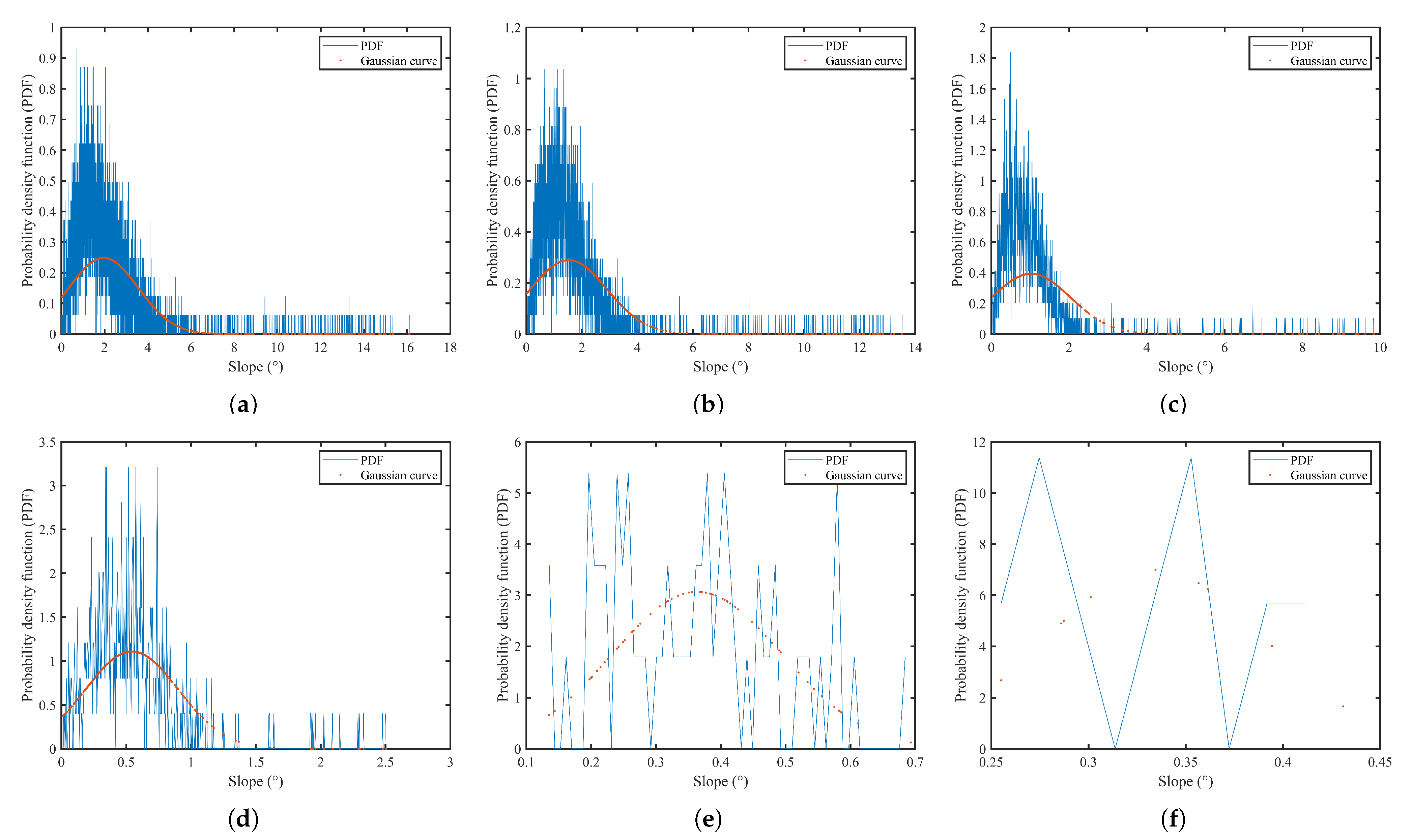
2.3. Scale-Effect Evaluation Factor

Albedo is a measurement scale for how much solar radiation a surface area reflects. Generally speaking, we think that the topography of a particular place is described more accurately with the higher spatial resolution. The scale with the 60 m spatial resolution preserves the majority of the texture detail and is the study’s most realistic portrayal of the lunar surface, as seen in Figure 1. As a result, the albedo results for this scale are used as the lunar reference albedo for other scales [10].

The scale-effect evaluation factor of the terrain’s albedo is therefore defined as the relative inaccuracy between reference albedo and other scale albedos, and it can be written as follows:

$$\delta =\frac{|a_{app}-a_{ref}|}{a_{ref}}\times 100\%$$

(13)

$a_{ref}$ is the albedo of the highest spatial resolution (i.e., 60 m) calculated based on the MRRT model, and $a_{app}$ represents the albedo calculated by other scales based on MRRT. We call the relative error $\delta$ the scale-effect evaluation factor of the albedo of the terrain. The closer the value of $\delta$ is to zero, the less the actual albedo in the region is affected by the scale effect.

2.4. Scale-Effect Function

In this paper, each pixel of DEM data in the target area constitutes a micro-topographic slope. Let b the scale factor between the microtopography and the target region, which can be expressed by the reciprocal of DEM spatial resolution t, i.e.,

$$b=\frac{1}{t}$$

(14)

The relationship between the scale-effect evaluation factor $\delta$ and b is described as follows.

$$f(\delta ,b)=p_{1}exp\left(p_{2}b\right)+p_{3}exp\left(p_{4}b\right)$$

(15)

$p_1$, $p_2$, $p_3$, and $p_4$ are all fitting parameters. Equation (15) expresses the relative error between the albedo at different scales and the actual albedo, which is mainly related to scale scaling factor between the microtopography and the target region. The closer the value of $f(\delta ,b)$ is to zero, the less the albedo in the region is affected by the scale effect.

3. Results

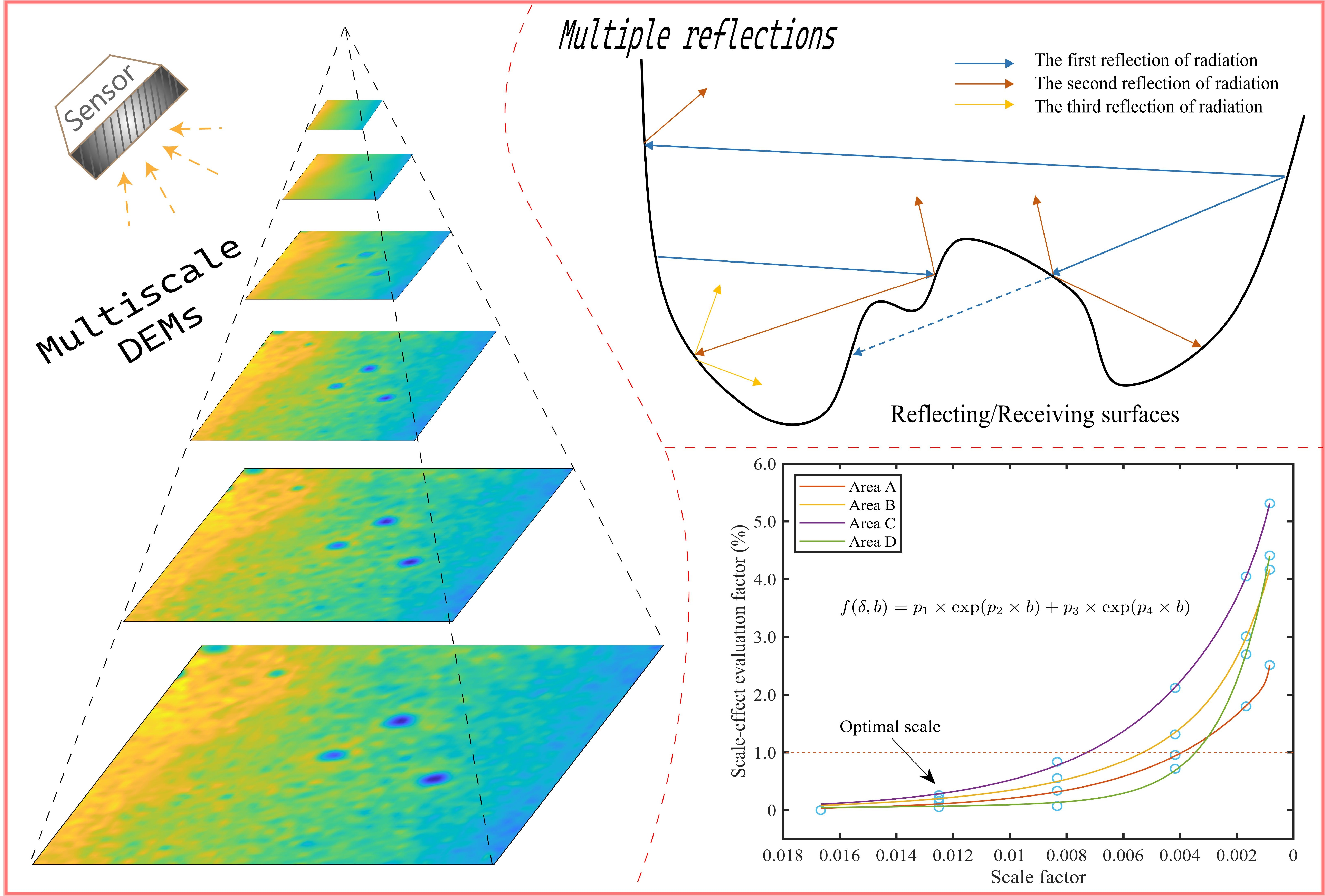
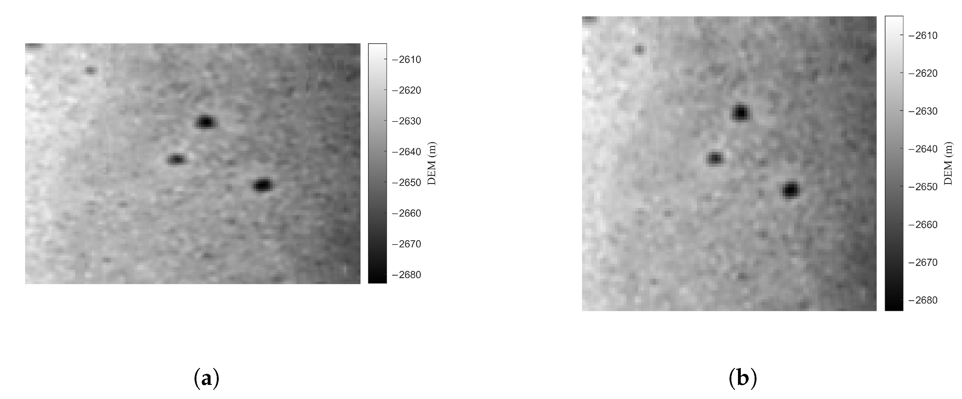
3.1. Multiscale Comparison of the Hapke Model and MRRT Model

Hapke [20,24] proposed the shadowing function to represent the influence of the shadow formed within the pixel due to topographic relief on the pixel reflectance. The pixel bidirectional reflectance (factor) with the impact of the topography inside the pixel can be expressed as follows:

$${\rho }_{BRF\_lowresolution}={\rho }_{e\_terrain}\times S(DEM,{\theta }_0,{\varphi }_0,{\theta }_v,{\phi }_v)$$

(16)

where $S(DEM,{\theta }_0,{\varphi }_0,{\theta }_v,{\phi }_v)$ is the shadowing function with the value 1 when there is no shadow and 0 when there is all shadow inside the pixel. When there is both shadow and illumination inside the pixel, the value of S is between 0 and 1.

For the convenience of comparison, Equation (11) is rewritten into the following form:

$$BRF({\theta }_0,{\varphi }_0,{\theta }_v,{\phi }_v)=\rho \times M(DEM,{\theta }_0,{\varphi }_0,{\theta }_v,{\phi }_v)$$

(17)

In Equation (17), $M(DEM,{\theta }_0,{\varphi }_0,{\theta }_v,{\phi }_v)$ is defined as the microtopography effect factor inside the target region, which comprehensively reflects the influence of micro-terrain on BRF of the target region. Based on the six various scales of DEM data, a comparison between the microtopography effect factor $M(DEM,{\theta }_0,{\varphi }_0,{\theta }_v,{\phi }_v)$ and the Hapke shadowing function $S(DEM,{\theta }_0,{\varphi }_0,{\theta }_v,{\phi }_v)$ has been made.

Figure 3 and Figure 4 illustrate the variation of the Hapke shadowing function and microtopography effect factor under various illumination observation geometries in the principal plane of the solar location at (0${}^{\circ }$, 150${}^{\circ }$) and (45${}^{\circ }$, 150${}^{\circ }$). The microtopographic surface’s reflectance is set to 0.15, and the solar incident irradiance is set at 100 W/m${}^2$.

Figure 3 demonstrates that the outcomes of various scales of DEM under various observation angles are always 1 when the solar zenith angle is 0${}^{\circ }$ (see Figure 3a). Different degrees of shadow masking develop in DEM zones of different scales under different observation angles when the solar zenith angle changes from 0${}^{\circ }$ to 45${}^{\circ }$. The shadowing function value shows a gradually declining trend as the spatial resolution of the terrain decreases, indicating that the region with the low spatial resolution has a greater proportion of shadows in the observation field of view under the same circumstances and that the microtopography effect is more significant. This outcome is in contrast to the illustration in Figure 2, which shows that a lower spatial resolution has a smaller average slope and standard deviation. The shadowing function was developed with the assumption that the slope of the terrain would have a Gaussian distribution, which is frequently not the case in reality. This may be the cause of the issue. In Appendix A.2, the fitted Gaussian function curve and the probability density function for each of the six groups of scale terrain slope are shown in Figure A3. The inaccuracy of the Gaussian function curve fitted by fewer DEM grid points increases as the topographic spatial resolution decreases.

Figure 4 demonstrates that as the spatial resolution decreases, the value of the microtopography effect factor gets closer to 1. This phenomenon shows that topographic relief is minimal at the low spatial resolution, which means that the BRF of the entire region is less affected by microtopography. As a result, the BRF is very close to the microtopography surface’s reflectance. This presentation is in line with the terrain’s decreasing average slope and standard deviation trend in Figure 2. Additionally, the microtopography effect factor of six scale DEMs is greater than 1 for the majority of observation angles. This phenomenon is said to be caused by the numerous reflections between terrains increasing the incident irradiance of the microtopographic surface, which then increases the reflected radiance in the observation direction [4]. According to Equation (11), the value of the denominator remains the same, and the numerator $L_v$ increases with the increase in the number of reflections between terrains, so the BRF increases. According to the calculation of literature [4], when the surface reflectance of microtopography is 0.15, the region’s BRF increases the percentage of different terrain is about 4% to 8%.

In addition, in Figure 4a,b, there was no significant difference in the microtopography effect factor for most observed zenith angles. At the same time, the difference in microtopography effect factors of these observed zenith angles at different scales is also small. This might be the case because, as shown in Figure 2, the average slope of the six scale DEMs for the Chang’e-3 landing region changed from 1.980472 to 0.334923, indicating that the landscape is relatively flat. Thus, the reflected radiance observed from most viewing angles is similar. The distribution of irradiance on the Chang’e-3 landing region for two sun incidence angles is displayed in Figure 5. It is obvious that the irradiance is distributed evenly. Additionally, Figure 4 shows little change in the scale effect for flatter regions at most observational angles; the enlarged image shows that the microtopography effect factor values of the DEM grid of $100\times 100$ pixels, $75\times 75$ pixels, $50\times 50$ pixels, and $25\times 25$ pixels are much closer, which demonstrates that the scale effect is minimal in the DEM of these four scales.

The slope is assumed to be Gaussian distribution in the Hapke model, which results in significant inaccuracies. The MRRT model, in contrast, does not relate to this assumption. The MRRT model’s microtopography effect factor can more accurately reflect the microtopography’s impact on the BRF over the entire region, making it better suited for identifying scale-effect changes in the actual terrain.

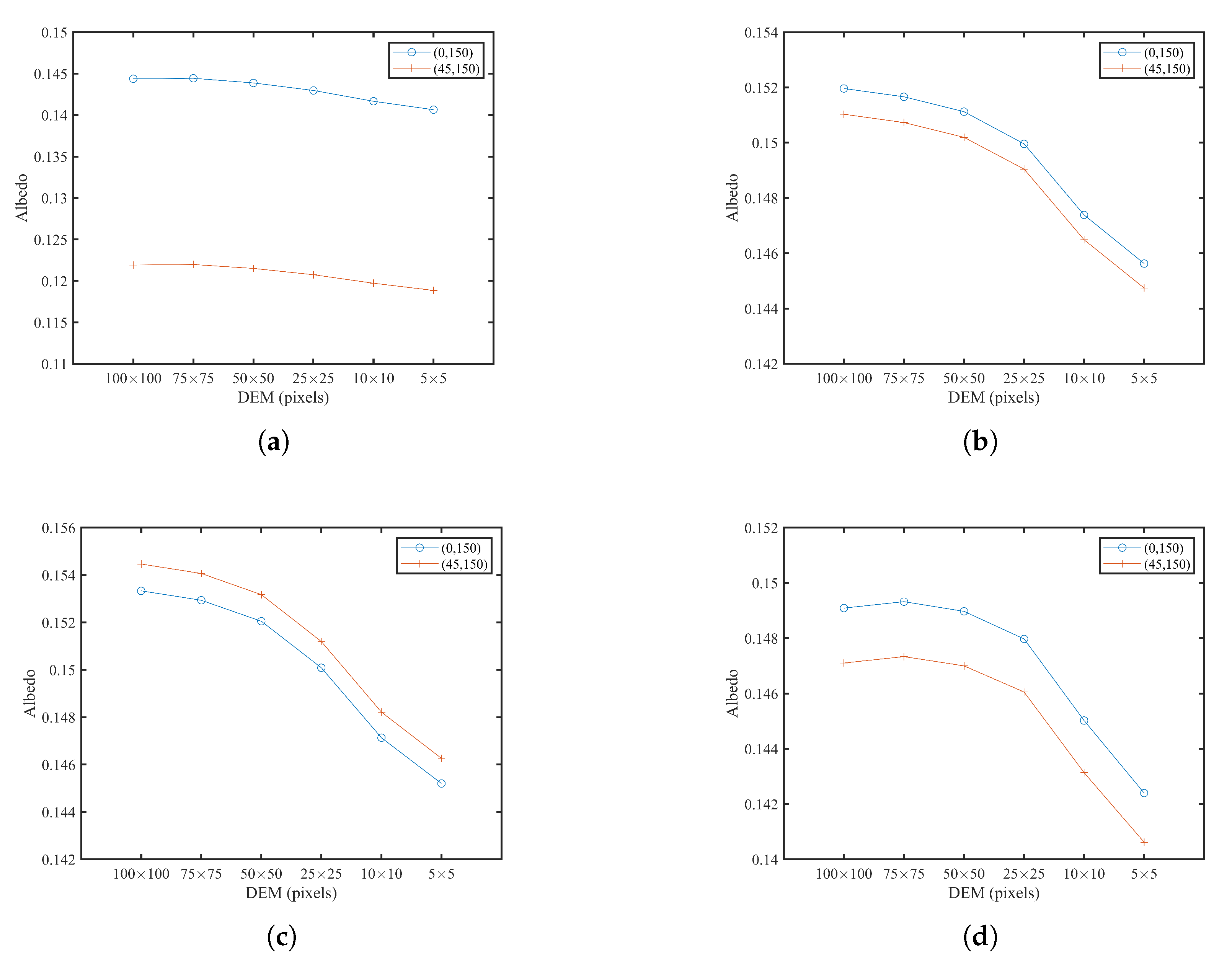
3.2. Albedo of Multiscale DEMs Based on the MRRT Model

The albedo is determined at various scales for the landscape in the Chang’e-3 landing region using the MRRT model. The Lambert reflectance of the microtopographic surface is assumed to be 0.15, and the solar incident irradiance is set as 100 W/m${}^2$. Figure 6 shows the regional albedo at different scales in two solar incident angles of (0${}^{\circ }$, 150${}^{\circ }$) and (45${}^{\circ }$, 150${}^{\circ }$).

As shown in Figure 6, in the DEM grid of $100\times 100$ pixels, $75\times 75$ pixels, and $50\times 50$ pixels, the albedo under the two groups of solar incidence angles is more than 0.15. This is due to the fact that multiple reflections between terrains enhance the microtopographic surface’s incidence irradiance, which raises the total amount of reflected radiation. As a result, the albedo result can exceed 0.15. Additionally, the albedos at six scale DEMs under the solar incident angle of (45${}^{\circ }$, 150${}^{\circ }$) are much higher than they are under the solar incident angle of (0${}^{\circ }$, 150${}^{\circ }$). This indicates that due to the multiple reflections of radiation between the terrains, the ratio of total reflected radiation to incident radiation increases more at the solar incidence angle (45${}^{\circ }$, 150${}^{\circ }$) than at the solar incidence angle (0${}^{\circ }$, 150${}^{\circ }$). The solar incident angle and the actual terrain are connected to this phenomenon. There is no direct correlation between the magnitude of the terrain’s albedo at various incidence angles.

In the DEM grid of $100\times 100$ pixels, $75\times 75$ pixels, $50\times 50$ pixels and $25\times 25$ pixels, the albedo under the two groups of solar incidence angles differs greatly. In contrast, there is only a little difference in albedo between the DEM grids of $10\times 10$ pixels and $5\times 5$ pixels. This demonstrates that with the reduction of the spatial resolution of the terrain, the slope of the terrain becomes gentler, as shown in Figure 2, and the influence of the solar incident zenith angle on the albedo results decreases. Additionally, when the DEM grid is $25\times 25$ pixels, the albedo curve has a distinct turning point. To assess the scale impact of albedo, the scale-effect evaluation factor of albedo under the two sets of sun angles is computed.

The highest spatial resolution of the DEM in this paper, which is used to calculate the reference albedo $a_{ref}$, is 60 m, as was mentioned in Section 2.3. Figure 7 demonstrates how a second-order exponential function (see Equation (15)) can be used to express the relationship between the scale-effect evaluation factor and terrain scale factor. Six scale factors are, respectively, 1/60, 1/80, 1/120, 1/240, 1/600, and 1/1200. The calculated albedo is more closely related to the reference albedo the smaller the scale-effect evaluation factor is. It can be seen that there is a clear turning point at 1/240 based on the slope changes of the fitting curve at each scale factor, which is consistent with the outcome in Figure 6. Therefore, the scale critical point given by the curve is about $1/240$. Additionally, the Figure 7a,b show that under the two sets of sun incidence angles, the curves of the scale-effect function are similar, which demonstrates that for these two sets of incidence angles, the microtopographic impact of albedo varies evenly with the change in scale. This pattern suggests that the topography features of different scales are preserved reasonably uniformly in the topographic data obtained in this region. The information utilized in this paper’s calculations is therefore trustworthy.

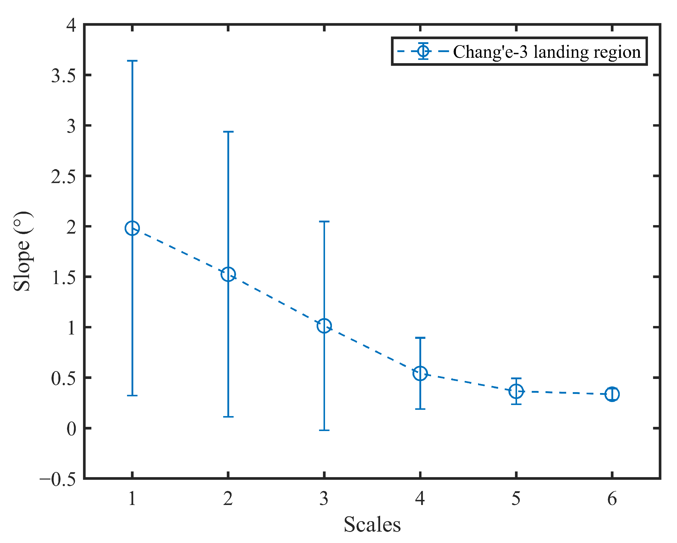
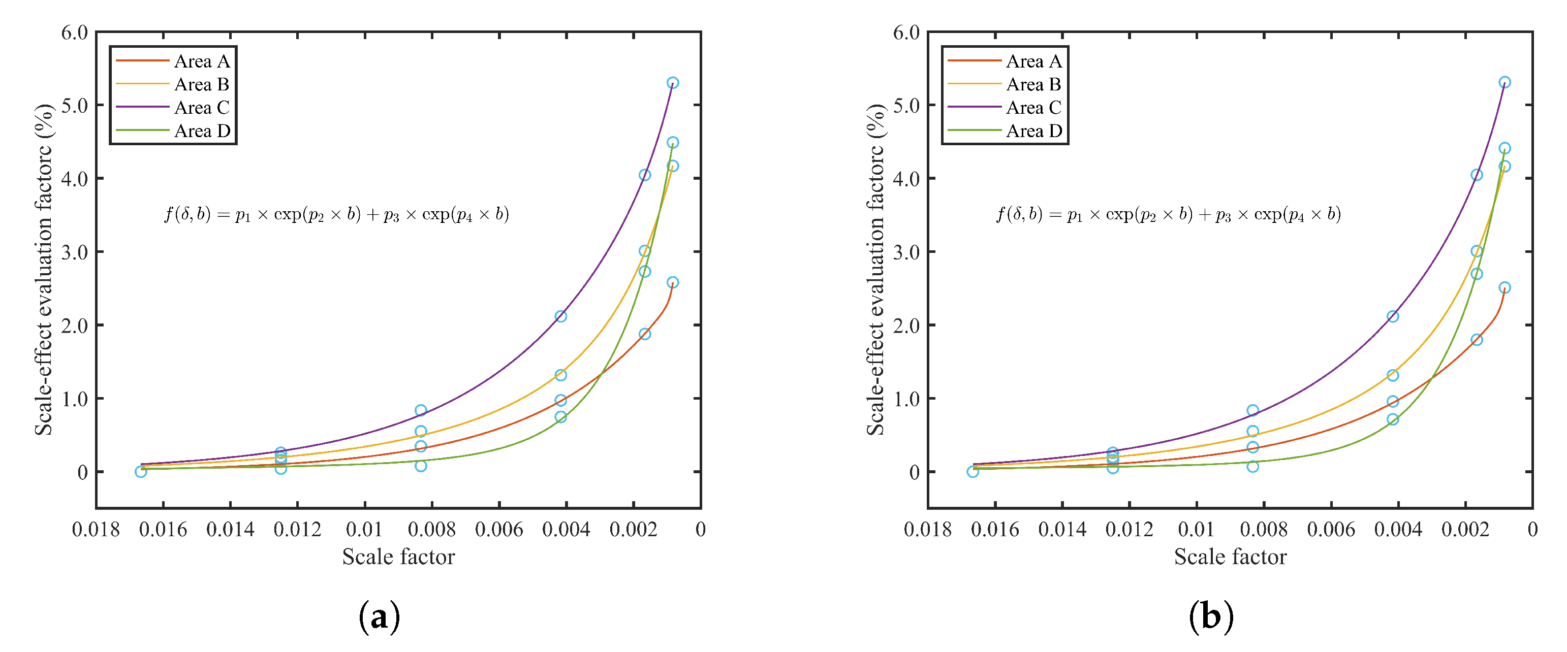
3.3. Applied on Other Lunar Regions

Four randomly selected lunar surface regions, each the same size as the Chang’e-3 landing zone, were processed in the same manner as in Appendix A.1. Figure 8 depicts the outcomes. The scale factors 1/60, 1/80, 1/120, 1/240, 1/600, and 1/1200 produce multiscale topography of regions, accordingly. The MRRT model is used to determine the albedo and scale-effect evaluation factors for the four landscapes at various scales.

The ordinate coordinates of the four groups of albedo figures are not unified in Figure 9 to better illustrate how albedo changes with scale. The albedo under the two groups of solar incident angles exhibits similar variation trends with scale in various terrains. The analysis of the results is consistent with that of Figure 6. A second-order exponential function can be used to explain the relationship between the scale-effect evaluation factor of various terrains and scale factors, as shown in Figure 10. For different regions, the scale-effect evaluation factor of albedo calculated by microtopography constructed with spatial resolution between 60 and 120 is less than 1%. Moreover, the scale-effect evaluation factors of different terrains at the same scale are similar. This indicates that the scale critical point given by the curve should be around $1/120$. Combining the findings of Section 3.2, this shows that it is acceptable to build a microtopography with a spatial resolution of 60 m to 120 m and perform albedo calculations for an area of (6000 × 6000) m${}^2$, in which the spatial resolution of 80 m is the most suitable scale.

4. Discussion

The moon has stable luminosity ideal for a calibration source. Radiometric calibration based on the lunar surface region is a favorable development direction with the enhancement of the observation capabilities of remote sensing devices [4]. The key to creating a radiation regional calibration model on the lunar surface, however, is to take into account the topographic effects and the heterogeneity of material distribution. Additionally, the majority of research demonstrates that the scale effect is the main factor contributing to uncertainty in albedo estimation, and the influence of topography on remote sensing data is scale-dependent [8]. Neglecting within-pixel topology could lead to mistakes in albedo estimation from coarse-scale data because of the scale effect in albedo [25].

Hapke [20,24] proposed the shadowing function to express the impact of the shadow created within the pixel due to topographic relief on the pixel reflectance. However, the shadowing function was developed with the assumption that the terrain’s slope adheres to the Gaussian distribution, which is frequently not the case (see Figure A3). The shadowing function in Figure 3b exhibits a trend toward steady decline as the terrain spatial resolution is reduced. This outcome is in contrast to the illustration in Figure 2, which shows that a lower spatial resolution has a smaller average slope and standard deviation. In contrast, the MRRT model [4] used Proy’s neighboring terrain irradiance formula [21] to derive the second-order to nth-order reflections of radiation between terrains, which established the relationship between the bidirectional reflectance factor (BRF) of the observed pixel and the genuine microtopography reflectance (see Equation (11)). The variation trend of the microtopography effect factor based on the MRRT model is depicted in Figure 4 and is compatible with the actual circumstance. This suggests that in order to determine the scale effect variations of the actual terrain, the MRRT model may more accurately explain the microtopography influence on the BRF of the entire region.

This work further derives the albedo formula from the MRRT model (see Equation (12)). Section 3.2 states that at the two sun incoming angles, the albedo findings derived at various scales preserve comparable change curves; the scale-effect evaluation factor and scale factor may be related using a fourth-order polynomial formula. It can be shown that the scale effect of albedo has a critical point of scale, meaning that increasing the DEM data needed to compute it or decreasing a particular fraction has very little impact on the actual albedo calculation. This judgment is supported in Section 3.3: Figure 10 demonstrates that the scale critical point indicated by the curve is approximately $1/120$ in the four parts of the lunar surface that were arbitrarily chosen. This shows that it is acceptable to build a microtopography with a spatial resolution of 60 m to 120 m and perform albedo calculations for an area of (6000 × 6000) m${}^2$, in which the spatial resolution of 80 m is the most suitable scale. According to the experimental findings, neither the tiniest nor the largest scale is the best scale. Using a known-size area, we may create multiscale DEMs and use MRRT to determine the albedo at various scales. We may obtain the best micro-topographic scale in this region by fitting the scale-effect function, which can then be used for MRRT modeling in other regions.

This research adds to the MRRT model’s applicability analysis in multiscale DEM modeling, helps choose and build a radiation calibration field on the lunar surface, and lays the groundwork for employing the area of the lunar surface for radiation calibration. However, the model accuracy of applying MRRT to the radiometric calibration field on the lunar surface has not been thoroughly assessed due to the limited lunar radiance observation data and in situ measured reflectance data. Additionally, the lunar soil made up of dust, noncohesive rocks, debris, and molten glass covers most of the lunar surface. The weathering of lunar rocks in space produces lunar soil [26]. At less than 1 cm of scale, the lunar surface’s relief becomes ambiguous, and the soil is porous. The size, shape, transparency, porosity, and surface roughness of the lunar soil particles all affect how reflective the materials on the lunar surface are [20]. In the MRRT model, it is considered that the reflectance of the microtopographic surface with larger than the particle level but smaller than the detector observation scale is the surface result of the comprehensive reflection of the radiation characteristics of light between the lunar soil particles, and it is assumed to be Lambertian body reflection. When attaining sufficiently high DEM spatial resolution, it is advised to try to employ the MRRT model in conjunction with other lunar surface photometric functions such as the Hapke function, Akimov function, or Shkuratov function [27,28].

A ground-based lunar observation system with a spatial resolution of the visible bands of 7 km was established by the Shanghai Institute of Technical Physics of the Chinese Academy of Sciences, and it has started to be seen. The instrument’s observation data will be used to help the MRRT model’s subsequent correction and accuracy assessment.

References

1. Stone, T.; Kieffer, H. Absolute Irradiance of the Moon for On-orbit Calibration. In Proceedings of the SPIE-The International Society for Optical Engineering, Seattle, WA, USA, 7–10 July 2002; Volume 4814. [Google Scholar] [CrossRef]
2. Stone, T.C.; Kieffer, H.H. Assessment of Uncertainty in ROLO Lunar Irradiance for On-Orbit Calibration. Proc. SPIE 2004, 5542, 300–310. [Google Scholar] [CrossRef]
3. Wagner, S.C.; Hewison, T.; Stone, T.; Lachérade, S.; Fougnie, B.; Xiong, X. A Summary of the Joint GSICS – CEOS/IVOS Lunar Calibration Workshop: Moving towards Intercalibration Using the Moon as a Transfer Target. Proc. SPIE 2015, 9639, 96390Z. [Google Scholar] [CrossRef]
4. Liu, Y.; Guo, Q.; Wang, G. MRRT: Modeling of Multiple Reflections of Radiation between Terrains Applied on the Lunar Surface Region. IEEE Trans. Geosci. Remote Sens. 2022, 60, 5413417. [Google Scholar] [CrossRef]
5. Li, X.W.; Wang, Y.T. Prospects on Future Developments of Quantitative Remote Sensing. J. Geogr. Sci. 2013, 68, 1163–1169. [Google Scholar]
6. Li, X.W. Retrospect, Prospect and Innovation in Quantitative Remote Sensing. J. Henan Univ. Nat. Sci. 2005, 35, 49–56. [Google Scholar]
7. Wu, X.; Wen, J.; Xiao, Q.; You, D.; Gong, B.; Wang, J.; Ma, D.; Lin, X. Spatial Heterogeneity of Albedo at Subpixel Satellite Scales and Its Effect in Validation: Airborne Remote Sensing Results From HiWATER. IEEE Trans. Geosci. Remote Sens. 2022, 60, 21532871. [Google Scholar] [CrossRef]
8. Wen, J.; Liu, Q.; Xiao, Q.; Liu, Q.; You, D.; Hao, D.; Wu, S.; Lin, X. Characterizing Land Surface Anisotropic Reflectance over Rugged Terrain: A Review of Concepts and Recent Developments. Remote Sens. 2018, 10, 370. [Google Scholar] [CrossRef] [Green Version]
9. Wu, X.; Wen, J.; Xiao, Q.; You, D.; Wang, J.; Ma, D.; Lin, X. A Multiscale Nested Sampling Method for Representative Albedo Observations at Various Pixel Scales. IEEE J. Sel. Top. Appl. Earth Obs. Remote Sens. 2021, 14, 8193–8207. [Google Scholar] [CrossRef]
10. Zeng, X.; Li, C. The Influence of Heterogeneity on Lunar Irradiance Based on Multiscale Analysis. Remote Sens. 2019, 11, 2696. [Google Scholar] [CrossRef] [Green Version]
11. McEwen, A.; Eliason, E.; Lucey, P.; Malaret, E.; Pieters, C.; Robinson, M.; Sucharski, T. Summary of Radiometric Calibration and Photometric Normalization Steps for the Clementine UVVIS Images. In Proceedings of the 29th Annual Lunar and Planetary Science Conference, Houston, TX, USA, 1 March 1998; p. 1466. [Google Scholar]
12. Yokota, Y.; Matsunaga, T.; Ohtake, M.; Haruyama, J.; Nakamura, R.; Yamamoto, S.; Ogawa, Y.; Morota, T.; Honda, C.; Saiki, K.; et al. Lunar Photometric Properties at Wavelengths 0.5–1.6μm Acquired by SELENE Spectral Profiler and Their Dependency on Local Albedo and Latitudinal Zones. Icarus 2011, 215, 639–660. [Google Scholar] [CrossRef]
13. Wu, Y.; Besse, S.; Li, J.Y.; Combe, J.P.; Wang, Z.; Zhou, X.; Wang, C. Photometric Correction and In-Flight Calibration of Chang’ E-1 Interference Imaging Spectrometer (IIM) Data. Icarus 2013, 222, 283–295. [Google Scholar] [CrossRef]
14. Wu, Y.; Hu, X.; Li, S. The Irradiance Model of the Moon and Its Implication on the On-orbit Calibration of Spacecraft. In Proceedings of the 4th Annual Conference on High Resolution Earth Observation, Wuhan, China, 17 September 2017; p. 9. [Google Scholar]
15. Chen, S.B.; Wang, J.R.; Guo, P.J.; Wang, M.C. Sandmeier Model Based Topographic Correction to Lunar Spectral Profiler (SP) Data from KAGUYA Satellite. Spectrosc. Spectr. Anal. 2014, 34, 2573–2577. [Google Scholar] [CrossRef]
16. Shepherd, J.D.; Dymond, J.R. Correcting Satellite Imagery for the Variance of Reflectance and Illumination with Topography. Int. J. Remote Sens. 2003, 24, 3503–3514. [Google Scholar] [CrossRef]
17. Sandmeier, S.; Itten, K.I.J.G. A Physically-Based Model to Correct Atmospheric and Illumination Effects in Optical Satellite Data of Rugged Terrain. IEEE Trans. Geosci. Remote Sens. 1997, 35, 708–717. [Google Scholar] [CrossRef] [Green Version]
18. Hapke, B.W. A Theoretical Photometric Function for the Lunar Surface. J. Geophys. Res. 1963, 68, 4571–4586. [Google Scholar] [CrossRef]
19. Xu, X.; Liu, J.; Liu, D.; Liu, B.; Shu, R. Photometric Correction of Chang’E-1 Interference Imaging Spectrometer’s (IIM) Limited Observing Geometries Data with Hapke Model. Remote Sens. 2020, 12, 3676. [Google Scholar] [CrossRef]
20. Hapke, B. Theory of Reflectance and Emittance Spectroscopy, 2nd ed.; United States of America by Cambridge University Press: New York, NY, USA, 2012. [Google Scholar]
21. Proy, C.; Tanre, D.; Deschamps, P. Evaluation of Topographic Effects in Remotely Sensed Data. Remote Sens. Environ. 1989, 30, 21–32. [Google Scholar] [CrossRef]
22. Barker, M.; Mazarico, E.; Neumann, G.; Zuber, M.; Haruyama, J.; Smith, D. A New Lunar Digital Elevation Model from the Lunar Orbiter Laser Altimeter and SELENE Terrain Camera. Icarus 2016, 273, 346–355. [Google Scholar] [CrossRef] [Green Version]
23. Shannon, C.E. A Mathematical Theory of Communication. Bell Syst. Tech. J. 1948, 27, 379–423. [Google Scholar] [CrossRef] [Green Version]
24. Hapke, B. Bidirectional Reflectance Spectroscopy: 3. Correction for Macroscopic Roughness. Icarus 1984, 59, 41–59. [Google Scholar] [CrossRef] [Green Version]
25. Wen, J.; Liu, Q.; Liu, Q.; Xiao, Q.; Li, X. Scale Effect and Scale Correction of Land-Surface Albedo in Rugged Terrain. Int. J. Remote Sens. 2009, 30, 5397–5420. [Google Scholar] [CrossRef]
26. Ouyang, Z. Introduction to Lunar Science; China Aerospace Publishing House: Beijing, China, 2005. [Google Scholar]
27. Shkuratov, Y.; Kreslavsky, M.; Ovcharenko, A.; Stankevich, D.; Zubko, E.; Pieters, C.; Arnold, G. Opposition Effect from Clementine Data and Mechanisms of Backscatter. Icarus 1999, 141, 132–155. [Google Scholar] [CrossRef] [Green Version]
28. Shkuratov, Y.; Kaydash, V.; Korokhin, V.; Velikodsky, Y.; Opanasenko, N.; Videen, G. Optical Measurements of the Moon as a Tool to Study Its Surface. Planet. Space Sci. 2011, 59, 1326–1371. [Google Scholar] [CrossRef]
Figure 1. Chang’e-3 landing region. The data from the lunar orbital laser altimeter (LOLA) used to create the multiscale digital elevation models (DEMs): (a) 60 m per pixel, (b) 80 m per pixel, (c) 120 m per pixel, (d) 240 m per pixel, (e) 600 m per pixel, (f) 1200 m per pixel.
Remotesensing 15 01158 g001
Figure 2. The topographic slope’s averages and standard deviations at six different scales. The labels “1” to “6” of the horizontal axis correspond to the subfigures (a) to (f) of Figure 1.
Remotesensing 15 01158 g002
Figure 3. Hapke model. Variation of the shadowing function under various illumination observations of the solar location’s primary plane: (a) (0 , 150 ) and (b) (45 , 150 ).
Remotesensing 15 01158 g003
Figure 4. MRRT model. Variation of the microtopography effect factor under various illumination observations of the solar location’s primary plane: (a) (0 , 150 ) and (b) (45 , 150 ). MRRT: multiple reflections of radiation between terrains.
Remotesensing 15 01158 g004
Figure 5. Irradiance distribution of the Chang’e-3 landing area under various solar locations: (a) (0 , 150 ) and (b) (45 , 150 ).
Remotesensing 15 01158 g005
Figure 6. Albedo of multiscale DEMs based on the MRRT model under different illumination geometry: (0 , 150 ) and (45 , 150 ).
Remotesensing 15 01158 g006
Figure 7. Scale-effect evaluation factor of multiscale DEMs based on the MRRT model under different illumination geometry: (a) (0 , 150 ) and (b) (45 , 150 ). Six scale factors are 1/60, 1/80, 1/120, 1/240, 1/600, 1/1200, respectively.
Remotesensing 15 01158 g007
Figure 8. Four arbitrarily selected regions on the lunar surface: (a) Area A: (23.7 N, 47 W), (b) Area B: (10 S, 0 E), (c) Area C: (20 N, 10 E), and (d) Area D: (16 N, 26 W). The DEM has a spatial resolution of 60 m in every region.
Remotesensing 15 01158 g008
Figure 9. Albedo of four lunar surface regions at different scales: (a) Area A, (b) Area B, (c) Area C, and (d) Area D. The ordinate coordinates of the four groups of albedo figures are not unified.
Remotesensing 15 01158 g009
Figure 10. Scale-effect evaluation factor of multiscale DEMs of four lunar regions based on the MRRT model under different illumination geometry: (a) (0 , 150 ) and (b) (45 , 150 ). Six scale factors are 1/60, 1/80, 1/120, 1/240, 1/600, and 1/1200, respectively.
Remotesensing 15 01158 g010