


Airborne Streak Tube Imaging LiDAR Processing System: A Single Echo Fast Target Extraction Implementation

 ,
,
Abstract
:1. Introduction
2. Background Knowledge
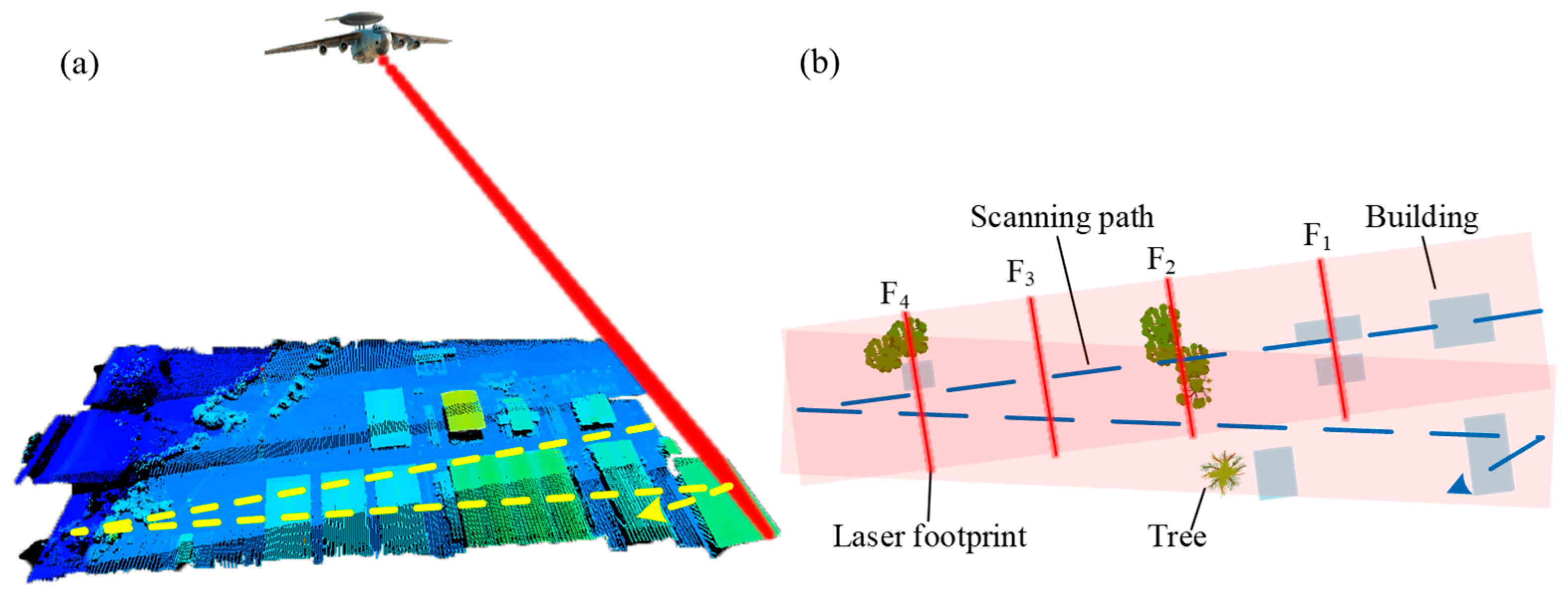
2.1. Airborne Streak Tube Imaging LiDAR
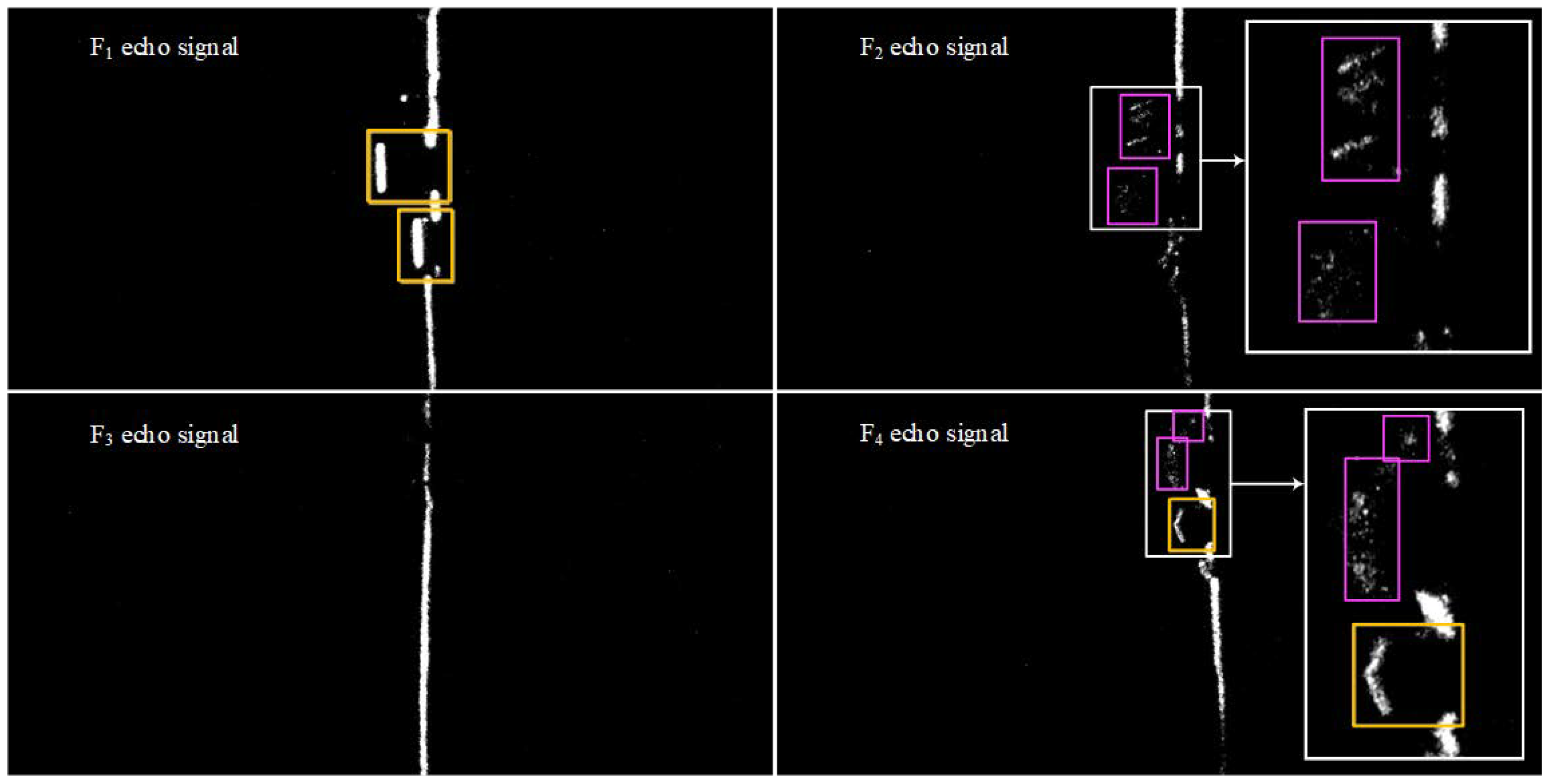
2.2. Data Collection and Annotation
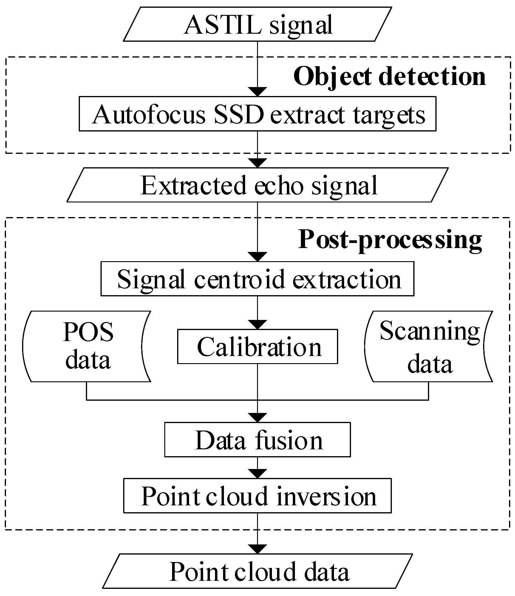
3. ASTIL Echo Signal Fast-Processing System
3.1. Autofocus SSD Network
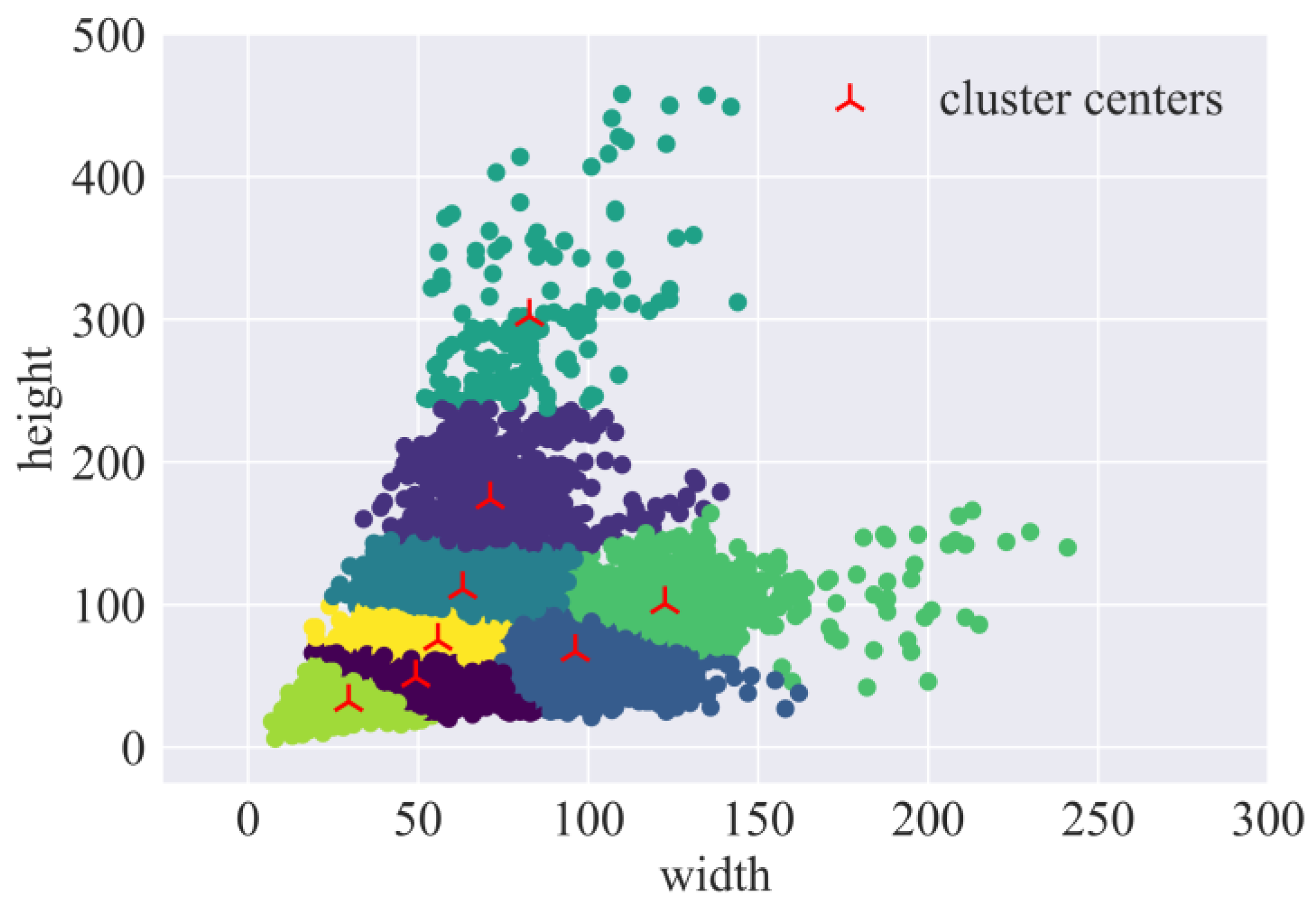
3.1.1. Hierarchical Setting of Default Box Size Based on K-Means
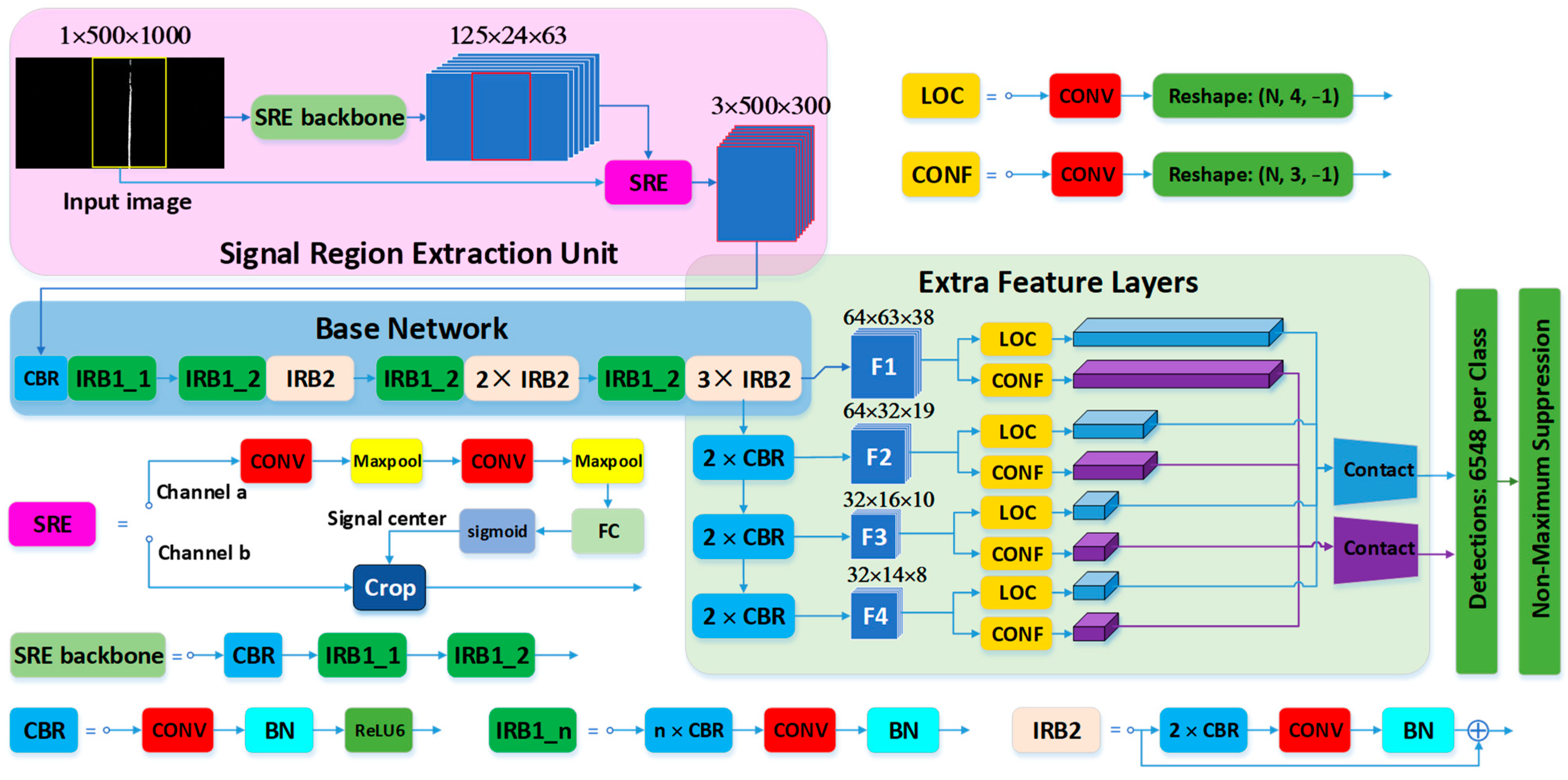
3.1.2. Architecture
3.1.3. Signal Region Extraction Unit
3.1.4. Streamlining the Base Network
3.1.5. Loss Function
3.2. Post-Processing of the Echo Signal
3.2.1. Signal Centroid Extraction
| Algorithm 1: Signal centroid extraction |
| Input: Extracted echo signal Output: Echo streak centroid
|
3.2.2. Calibration
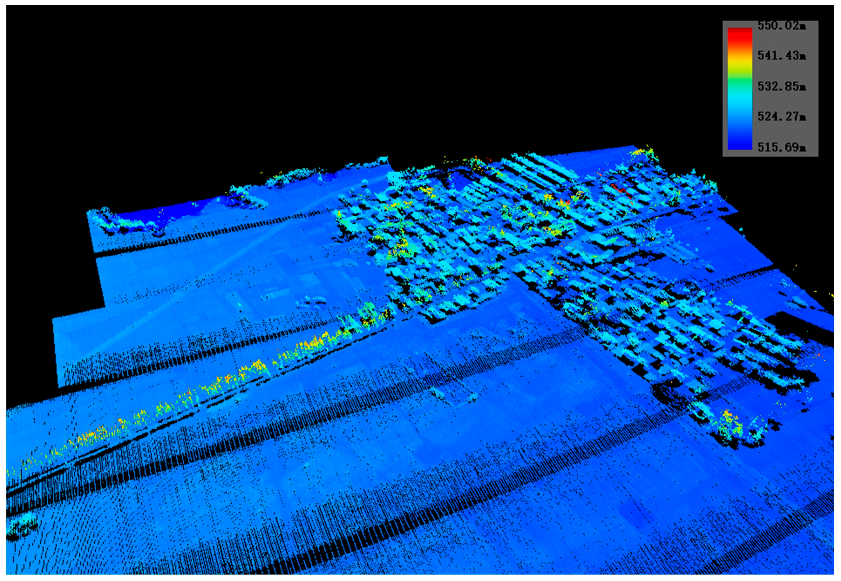
3.2.3. Data Fusion
4. Experiment and Results
4.1. Network Training Strategy
4.1.1. Autofocus SSD
4.1.2. Other Networks
4.1.3. Evaluation Metrics
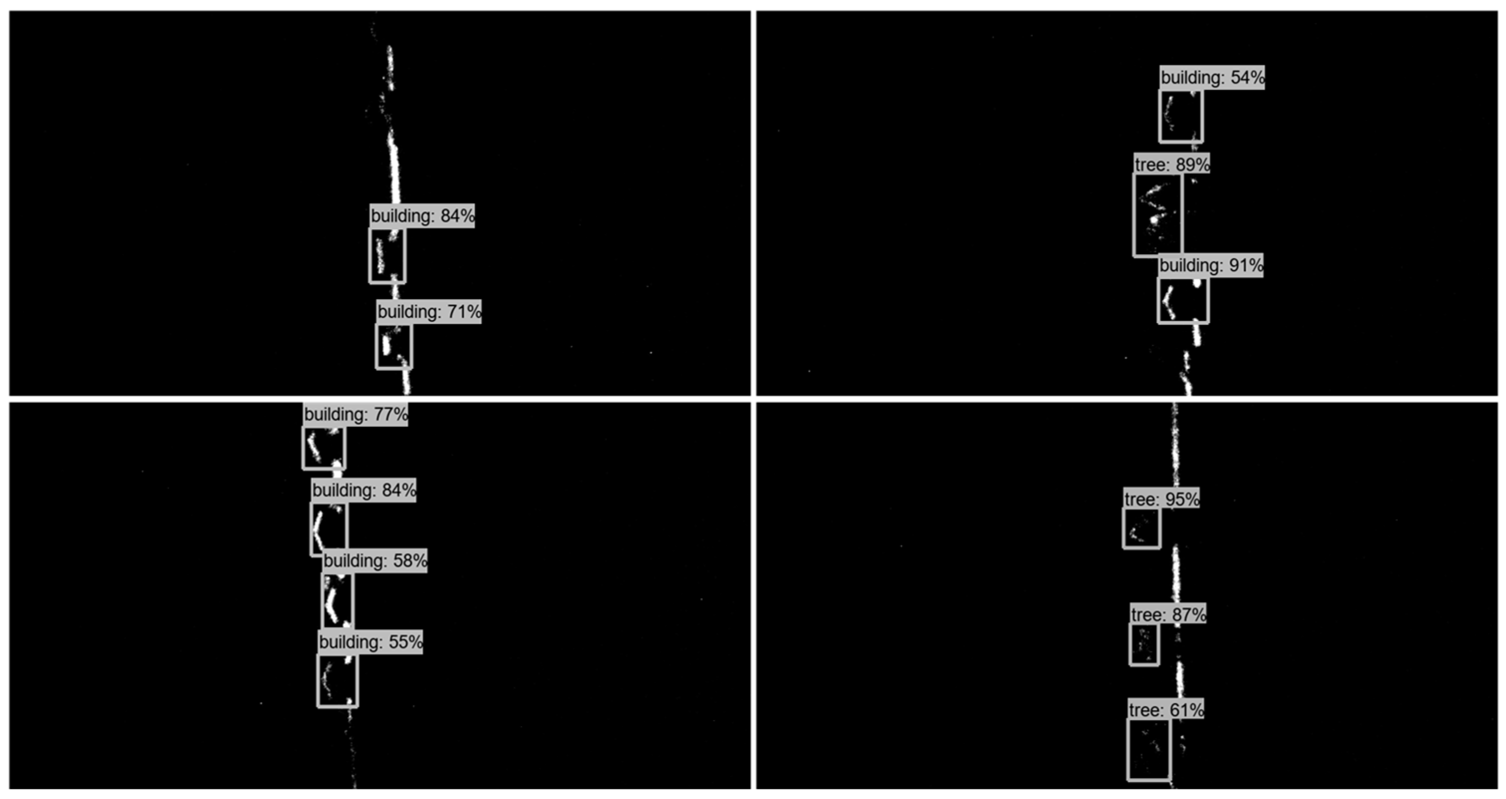
4.2. Echo Signal Detection Result
4.3. Autofocus SSD Analysis
4.3.1. Compared with Baseline Methods
- The feature extraction networks of these models were replaced with the same networks;
- The input image sizes for these models were all set to (3, 500, 1000);
- The data enhancement techniques for these models were retained and were not set to be identical;
- ASTIL has fewer foreground targets, and Faster RCNN extracted only a small number of proposals, reducing its prediction elapsed time.
4.3.2. Ablation Study
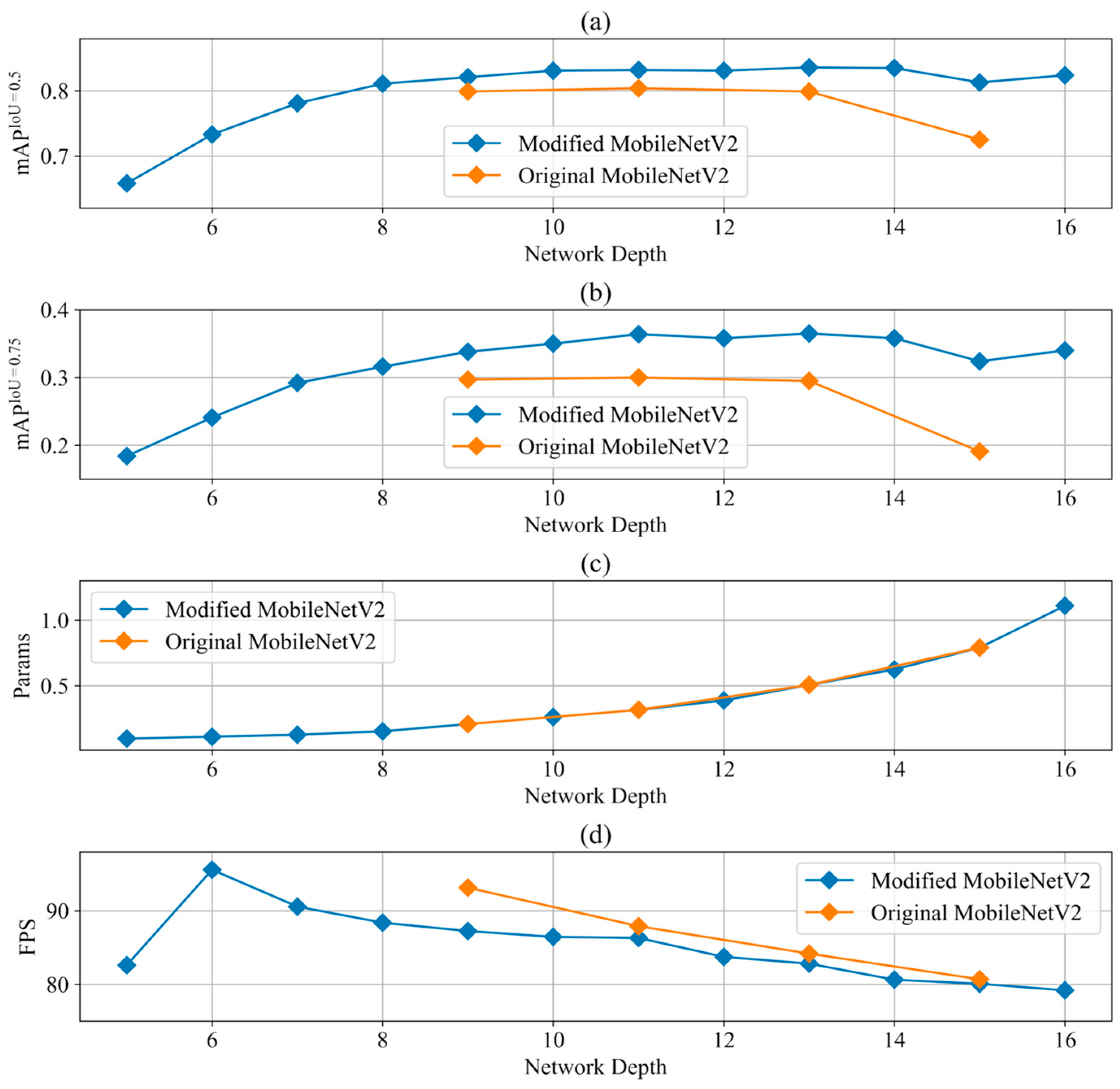
4.3.3. Base Network Structure Selection
4.4. ASTIL Fast-Processing System Evaluation
5. Conclusions
Author Contributions
Funding
Data Availability Statement
Conflicts of Interest
References
- Hang, R.L.; Li, Z.; Ghamisi, P.; Hong, D.F.; Xia, G.Y.; Liu, Q.S. Classification of Hyperspectral and LiDAR Data Using Coupled CNNs. IEEE Trans. Geosci. Remote Sens. 2020, 58, 4939–4950. [Google Scholar] [CrossRef] [Green Version]
- Zhao, X.D.; Tao, R.; Li, W.; Li, H.C.; Du, Q.; Liao, W.Z.; Philips, W. Joint Classification of Hyperspectral and LiDAR Data Using Hierarchical Random Walk and Deep CNN Architecture. IEEE Trans. Geosci. Remote Sens. 2020, 58, 7355–7370. [Google Scholar] [CrossRef]
- Zhou, R.Q.; Jiang, W.S. A Ridgeline-Based Terrain Co-registration for Satellite LiDAR Point Clouds in Rough Areas. Remote Sens. 2020, 12, 2163. [Google Scholar] [CrossRef]
- Huang, J.; Stoter, J.; Peters, R.; Nan, L.L. City3D: Large-Scale Building Reconstruction from Airborne LiDAR Point Clouds. Remote Sens. 2022, 14, 2254. [Google Scholar] [CrossRef]
- Liu, X.J.; Ning, X.G.; Wang, H.; Wang, C.G.; Zhang, H.C.; Meng, J. A Rapid and Automated Urban Boundary Extraction Method Based on Nighttime Light Data in China. Remote Sens. 2019, 11, 1126. [Google Scholar] [CrossRef] [Green Version]
- Pirotti, F. Analysis of full-waveform LiDAR data for forestry applications: A review of investigations and methods. iForest 2011, 4, 100–106. [Google Scholar] [CrossRef] [Green Version]
- Li, X.; Chen, W.Y.; Sanesi, G.; Lafortezza, R. Remote Sensing in Urban Forestry: Recent Applications and Future Directions. Remote Sens. 2019, 11, 1144. [Google Scholar] [CrossRef] [Green Version]
- Guo, B.; Li, Q.Q.; Huang, X.F.; Wang, C.S. An Improved Method for Power-Line Reconstruction from Point Cloud Data. Remote Sens. 2016, 8, 36. [Google Scholar] [CrossRef] [Green Version]
- Arastounia, M.; Lichti, D.D. Automatic Object Extraction from Electrical Substation Point Clouds. Remote Sens. 2015, 7, 15605–15629. [Google Scholar] [CrossRef] [Green Version]
- Huang, X.M.; Gong, J.; Chen, P.F.; Tian, Y.Q.; Hu, X. Towards the adaptability of coastal resilience: Vulnerability analysis of underground gas pipeline system after hurricanes using LiDAR data. Ocean Coast. Manag. 2021, 209, 105694. [Google Scholar] [CrossRef]
- Liu, Q.R.; Ruan, C.Q.; Guo, J.T.; Li, J.; Lian, X.H.; Yin, Z.H.; Fu, D.; Zhong, S. Storm Surge Hazard Assessment of the Levee of a Rapidly Developing City-Based on LiDAR and Numerical Models. Remote Sens. 2020, 12, 3723. [Google Scholar] [CrossRef]
- Wang, H.Z.; Glennie, C. Fusion of waveform LiDAR data and hyperspectral imagery for land cover classification. ISPRS J. Photogramm. Remote Sens. 2015, 108, 1–11. [Google Scholar] [CrossRef]
- Singh, K.K.; Vogler, J.B.; Shoemaker, D.A.; Meentemeyer, R.K. LiDAR-Landsat data fusion for large-area assessment of urban land cover: Balancing spatial resolution, data volume and mapping accuracy. ISPRS J. Photogramm. Remote Sens. 2012, 74, 110–121. [Google Scholar] [CrossRef]
- Wang, Y.L.; Li, M.S. Urban Impervious Surface Detection From Remote Sensing Images A review of the methods and challenges. IEEE Geosci. Remote Sens. Mag. 2019, 7, 64–93. [Google Scholar] [CrossRef]
- Nevis, A.J. Automated processing for Streak Tube Imaging Lidar data. In Proceedings of the Society of Photo-Optical Instrumentation Engineers, Orlando, FL, USA, 11 September 2003; pp. 119–129. [Google Scholar] [CrossRef]
- Axelsson, P. DEM Generation from Laser Scanner Data Using Adaptive TIN Models. Int. Arch. Photogramm. Remote Sens. 2000, 33, 110–117. [Google Scholar]
- Dong, Z.W.; Yan, Y.J.; Jiang, Y.G.; Fan, R.W.; Chen, D.Y. Ground target extraction using airborne streak tube imaging LiDAR. J. Appl. Remote Sens. 2021, 15, 16509. [Google Scholar] [CrossRef]
- Yan, Y.J.; Wang, H.Y.; Dong, Z.W.; Chen, Z.D.; Fan, R.W. Extracting suburban residential building zone from airborne streak tube imaging LiDAR data. Measurement 2022, 199, 111488. [Google Scholar] [CrossRef]
- Zhang, S.; Bogus, S.M.; Lippitt, C.D.; Kamat, V.; Lee, S. Implementing Remote-Sensing Methodologies for Construction Research: An Unoccupied Airborne System Perspective. J. Constr. Eng. Manag. 2022, 148, 03122005. [Google Scholar] [CrossRef]
- Redmon, J.; Divvala, S.; Girshick, R.; Farhadi, A. You Only Look Once: Unified, Real-Time Object Detection. In Proceedings of the 2016 IEEE Conference on Computer Vision and Pattern Recognition (CVPR), Las Vegas, NV, USA, 27–30 June 2016; pp. 779–788. [Google Scholar] [CrossRef] [Green Version]
- Liu, W.; Anguelov, D.; Erhan, D.; Szegedy, C.; Reed, S.; Fu, C.-Y.; Berg, A.C. SSD: Single Shot MultiBox Detector. In Proceedings of the European Conference on Computer Vision (ECCV), Amsterdam, The Netherlands, 8–16 October 2016; pp. 21–37. [Google Scholar] [CrossRef] [Green Version]
- Li, Z.; Wang, Y.C.; Zhang, N.; Zhang, Y.X.; Zhao, Z.K.; Xu, D.D.; Ben, G.L.; Gao, Y.X. Deep Learning-Based Object Detection Techniques for Remote Sensing Images: A Survey. Remote Sens. 2022, 14, 2385. [Google Scholar] [CrossRef]
- Hou, B.; Ren, Z.; Zhao, W.; Wu, Q.; Jiao, L. Object Detection in High-Resolution Panchromatic Images Using Deep Models and Spatial Template Matching. IEEE Trans. Geosci. Remote Sens. 2020, 58, 956–970. [Google Scholar] [CrossRef]
- Fan, Q.C.; Chen, F.; Cheng, M.; Lou, S.L.; Xiao, R.L.; Zhang, B.; Wang, C.; Li, J. Ship Detection Using a Fully Convolutional Network with Compact Polarimetric SAR Images. Remote Sens. 2019, 11, 2171. [Google Scholar] [CrossRef] [Green Version]
- Alganci, U.; Soydas, M.; Sertel, E. Comparative Research on Deep Learning Approaches for Airplane Detection from Very High-Resolution Satellite Images. Remote Sens. 2020, 12, 458. [Google Scholar] [CrossRef] [Green Version]
- Salari, A.; Djavadifar, A.; Liu, X.R.; Najjaran, H. Object recognition datasets and challenges: A review. Neurocomputing 2022, 495, 129–152. [Google Scholar] [CrossRef]
- Tong, K.; Wu, Y.Q. Deep learning-based detection from the perspective of small or tiny objects: A survey. Image Vis. Comput. 2022, 123, 104471. [Google Scholar] [CrossRef]
- Kaur, J.; Singh, W. Tools, techniques, datasets and application areas for object detection in an image: A review. Multimed. Tools Appl. 2022, 81, 38297–38351. [Google Scholar] [CrossRef]
- Sandler, M.; Howard, A.G.; Zhu, M.; Zhmoginov, A.; Chen, L.-C. MobileNetV2: Inverted Residuals and Linear Bottlenecks. In Proceedings of the 2018 IEEE/CVF Conference on Computer Vision and Pattern Recognition, Salt Lake City, UT, USA, 18–23 June 2018; pp. 4510–4520. [Google Scholar] [CrossRef] [Green Version]
- Liang, Y.; Ge, C.; Tong, Z.; Song, Y.; Wang, J.; Xie, P. Not All Patches are What You Need: Expediting Vision Transformers via Token Reorganizations. Available online: https://ui.adsabs.harvard.edu/abs/2022arXiv220207800L (accessed on 1 February 2022).


| Item | Configuration Info |
|---|---|
| acquisition platform | Harbin Y-12 (fixed-wing aircraft) |
| laser wavelength | 532 nm |
| echo type | waveform sampling |
| training set acquisition time | 2014.8.18 14:00:00 |
| test set acquisition time | 2014.8.18 13:41:38 |
| Objects | Raw Training Set | Training Set | Test Set |
|---|---|---|---|
| tree | 9249 | 11,223 | 18,537 |
| building | 28,124 | 11,086 | 14,018 |
| Operator | |||||
|---|---|---|---|---|---|
| CONV | 24 | 16 | (3, 3) | 1 | none |
| Maxpool | -- | -- | (3, 3) | -- | -- |
| CONV | 16 | 8 | (3, 3) | 1 | none |
| Maxpool | -- | -- | (3, 3) | -- | -- |
| FC | 624 | 1 | -- | -- | -- |
| Method | Params | FPS | ||
|---|---|---|---|---|
| Faster RCNN | 0.827 | 82.32 M | 45.35 | -- |
| SSD | 0.842 | 13.57 M | 26.59 | -- |
| YOLOV5s | 0.787 | 2.92 M | 87.72 | -- |
| Autofocus SSD | 0.832 | 0.32 M | 84.54 | 0.933 |
| Components | SREU | ✕ | ✓ | ✓ |
| Depth | 19 | 19 | 11 | |
| Metrics | 0.683 | 0.740 | 0.832 | |
| 0.148 | 0.205 | 0.364 | ||
| Params | 2.99 M | 2.49 M | 0.32 M | |
| FPS | 72.93 | 74.10 | 86.31 | |
| MACs | 3.40 G | 1.28 G | 1.13 G |
| Network Depth | Feature Map Size | Params (M) | FPS | ||
|---|---|---|---|---|---|
| 5 | 0.658 | 0.184 | (63, 38), (32, 19), (16, 10), (14, 8), | 0.098 | 82.61 |
| 6 | 0.733 | 0.241 | 0.113 | 95.57 | |
| 7 | 0.781 | 0.292 | 0.128 | 90.57 | |
| 8 | 0.811 | 0.316 | 0.154 | 88.38 | |
| 9 | 0.821 | 0.338 | 0.209 | 87.25 | |
| 10 | 0.831 | 0.350 | 0.263 | 86.45 | |
| Autofocus SSD | 0.832 | 0.364 | 0.317 | 86.31 | |
| 12 | 0.831 | 0.358 | 0.389 | 83.74 | |
| 13 | 0.836 | 0.365 | 0.507 | 82.82 | |
| 14 | 0.835 | 0.358 | 0.625 | 80.64 | |
| 15 | 0.813 | 0.324 | 0.791 | 80.08 | |
| 16 | 0.824 | 0.340 | 1.110 | 79.20 |
| Depth | Feature Map Size | Params (M) | FPS | ||
|---|---|---|---|---|---|
| 9 | 0.799 | 0.297 | (32, 19), (16, 10), (8, 5), (6, 3) | 0.209 | 93.13 |
| 11 | 0.804 | 0.300 | (32, 19), (16, 10), (8, 5), (6, 3) | 0.317 | 87.91 |
| 13 | 0.799 | 0.295 | (32, 19), (16, 10), (8, 5), (6, 3) | 0.507 | 84.18 |
| 15 | 0.725 | 0.191 | (16, 10), (8, 5), (4, 3), (2, 1) | 0.791 | 80.69 |
| Model FPS | Sys FPS | |||
|---|---|---|---|---|
| Building | Tree | |||
| 0.812 | 0.295 | 86.31 | 34.82 | 39.22 |
Disclaimer/Publisher’s Note: The statements, opinions and data contained in all publications are solely those of the individual author(s) and contributor(s) and not of MDPI and/or the editor(s). MDPI and/or the editor(s) disclaim responsibility for any injury to people or property resulting from any ideas, methods, instructions or products referred to in the content. |
© 2023 by the authors. Licensee MDPI, Basel, Switzerland. This article is an open access article distributed under the terms and conditions of the Creative Commons Attribution (CC BY) license (https://creativecommons.org/licenses/by/4.0/).
Share and Cite
Yan, Y.; Wang, H.; Song, B.; Chen, Z.; Fan, R.; Chen, D.; Dong, Z. Airborne Streak Tube Imaging LiDAR Processing System: A Single Echo Fast Target Extraction Implementation. Remote Sens. 2023, 15, 1128. https://doi.org/10.3390/rs15041128
Yan Y, Wang H, Song B, Chen Z, Fan R, Chen D, Dong Z. Airborne Streak Tube Imaging LiDAR Processing System: A Single Echo Fast Target Extraction Implementation. Remote Sensing. 2023; 15(4):1128. https://doi.org/10.3390/rs15041128
Chicago/Turabian StyleYan, Yongji, Hongyuan Wang, Boyi Song, Zhaodong Chen, Rongwei Fan, Deying Chen, and Zhiwei Dong. 2023. "Airborne Streak Tube Imaging LiDAR Processing System: A Single Echo Fast Target Extraction Implementation" Remote Sensing 15, no. 4: 1128. https://doi.org/10.3390/rs15041128