Article

Fresh Yield Estimation of Spring Tea via Spectral Differences in UAV Hyperspectral Images from Unpicked and Picked Canopies

1
College of Artificial Intelligence, Hangzhou Dianzi University, Hangzhou 310018, China
2
Institute of Agricultural Remote Sensing & Information Application, Zhejiang University, Hangzhou 310058, China
3
Key Laboratory of Agricultural Remote Sensing and Information System, Hangzhou 310058, China
4
School of Information Engineering, Zhejiang University of Water Resources and Electric Power, Hangzhou 310018, China
*
Author to whom correspondence should be addressed.
Remote Sens. 2023, 15(4), 1100; https://doi.org/10.3390/rs15041100
Submission received: 19 December 2022 / Revised: 4 February 2023 / Accepted: 14 February 2023 / Published: 17 February 2023
(This article belongs to the Special Issue Within-Season Agricultural Monitoring from Remotely Sensed Data)

Abstract

:
At present, spring tea yield is mainly estimated through a manual sampling survey. Obtaining yield information is time consuming and laborious for the whole spring tea industry, especially at the regional scale. Remote sensing yield estimation is a popular method used in large-scale grain crop fields, and few studies on the estimation of spring tea yield from remote sensing data have been reported. This is a similar spectrum of fresh tea yield components to that of the tea tree canopy. In this study, two types of unmanned aerial vehicle (UAV) hyperspectral images from the unpicked and picked Anji white tea tree canopies are collected, and research on the estimation of the spring tea fresh yield is performed using the differences identified in the single and combined chlorophyll spectral indices (CSIs) or leaf area spectral indices (LASIs) while also considering the changes in the green coverage of the tea tree canopy by way of a linear or piecewise linear function. The results are as follows: (1) in the linear model with a single index variable (LMSV), the accuracy of spring tea fresh yield models based on the selected CSIs was better than that based on the selected LASIs as a whole, in which the model based on the curvature index (CUR) was the best with regard to the accuracy metrics; (2) compared to the LMSVs, the accuracy performance of the piecewise linear model with the same index variables (PLMSVs) was obviously improved, with an encouraging root mean square error (RMSE) and validation determination coefficient (VR2); and (3) in the piecewise model with the combined index variables (PLMCVs), its evaluation metrics are also improved, in which the best performance of them was the CUR&CUR model with a RMSE (124.602 g) and VR2 (0.625). It showed that the use of PLMSVs or PLMCVs for fresh tea yield estimation could reduce the vegetation index saturation of the tea tree canopy. These results show that the spectral difference discovered through hyperspectral remote sensing can provide the potential capability of estimating the fresh yield of spring tea on a large scale.

Graphical Abstract

1. Introduction

Tea is an important cash crop. The total global tea yield reached 5.098 million hectares, and the dry yield of tea was 6.269 million tons in 2020 [1]. The yield of Chinese dry tea was 3.062 million tons in 2021, which produced an output value of USD 41.48 billion and ranked first in the world; additionally, the yield of spring tea was about 1.6–1.8 million tons, with an output value of USD 24.13–26.96 billion [2]. Spring tea yield is an important agronomy parameter and is beneficial for adjusting the management of activities, including tea picking, employing tea pickers, frying spring tea, and managing sales, in addition to handling other links in the spring tea industry. However, the yield estimation of spring tea is mainly achieved through a manual sampling survey. Obtaining this yield information using the method above is time consuming and laborious for the spring tea industry, especially at the regional scale. A rapid method for the large-scale estimation of spring tea yield is urgently needed.
Remote sensing technology has real-time, non-destructive, and rapid characteristics for monitoring a plant’s growth state, stress status, and yield [3,4,5], establishing remote sensing yield estimation as one of the popular methods for crop yield surveying [6,7,8]. At present, hyperspectral remote sensing is regarded as an effective method for crop yield estimation based on the spectral indices that have been discovered by many researchers. Feng et al. analyzed the effect of different spectral indices on the yield estimation of winter wheat via canopy hyperspectral images collected using UDH-185 equipped with a UAV platform [9]. A good correlation between the spectral index from airborne hyperspectral images of winter wheat and its yield was found, and the established yield estimation model had high precision [10]. Hyperspectral images from the different growth stages of winter wheat were used for its estimation based on the vegetation index, and the results showed ideal accuracy [11]. Furthermore, the rice yield was hyperspectrally estimated with higher accuracy [12]. The biomass and coverage retrieved via hyperspectral indices (for example, chlorophyll spectral indices (CSIs) and leaf area spectral indices (LASIs)) were used for maize yield estimation [13]. Additionally, hyperspectral data were also applied in the yield estimation of potato [14] and soybean [15]. In the above research, the crop yield estimation model based on hyperspectral data that was used to calculate the spectral index achieved good yield estimation results, demonstrating why it is one of the popular methods for use on a large scale.
In the tea yield estimation field, the remote sensing estimation of tea yield was first reported for in situ monitoring, and then for wide-range remote sensing. Jin et al. reported that tea yield was estimated using statistical modeling of the NDVI on the whole canopy before and after harvest [16]. Phamchimai Phan et al. used the NDVI of the multitemporal Medium Resolution Imaging Spectrometer to monitor tea growth and estimate tea yield [17], and the spatial-temporal mixed stochastic forest model was used to estimate tea yield [18].
Compared with crop yield estimation, there has been little research on tea yield estimation based on remote sensing data, especially spring tea. In addition to being difficult, the reasons for this could be: (1) a good theoretical knowledge of grain yield, as well as a high correlation between the growth at the vegetative growth stage that can be well monitored and the grain yield of grain crops at the reproductive stage, is used for estimating the yield with remote sensing data [19,20], but the tea yield components (buds and young leaves) are a part of the tea tree canopy, and there is a relatively low correlation between the yield and the growth of the tea tree canopy; and (2) the spectrum of fresh tea yield components is similar to that of the tea tree canopy [21]. Thus, acquiring the spectrum of fresh tea yield components is a critical step in estimating the fresh yield of spring tea with remote sensing data.
Fortunately, the harvesting of spring tea is commonly performed through the manual picking of spring tea yield components, and the spectral difference between the unpicked and picked tea tree canopies is produced by these picked yield components. This also provides a chance to acquire the spectrum of fresh tea yield components. However, there is a saturation phenomenon using many spectral indices for extracting spectral characteristics in these high-coverage canopies, such as the NDVI and RVI [22,23,24,25,26,27,28]. The tea tree canopy in the spring-tea-picking stage has high coverage [29,30]. Therefore, there was a need to reduce saturation in the extraction of spectral characteristics using the vegetation index from unpicked and picked tea tree canopies with high coverage. Coincidentally, the saturation phenomenon could be solved if: (1) the vegetation index model was a piecewise function containing only a single vegetation index; or (2) the index in the vegetation index model was a combination of indices that contained two or more vegetation indices [31,32,33,34]. In this study, the change in the green coverage from the unpicked and picked tea tree canopy was used for building the piecewise function and combining the indices for the spring tea fresh yield estimation.
The vegetation index is regarded as a powerful tool for extracting plant spectral information [35,36,37] and is widely used for the inversion of plant biochemical components [38,39] and for determining biomass [40] and yield, such as by using chlorophyll spectral indices (CSIs) [41,42], leaf area spectral indices (LAIs) [43] and vegetation water indices [40,44]. In addition, the results from two preliminary experiments were found, which included (the second and third figures in Section 2.1.4): (1) a significant difference in the ratio value of chlorophyll a and b content from the tea yield components (the tea buds and young leaves) and the mature leaves (the main component of the spectral response of the tea tree canopy), and (2) a good correlation between the area of tea yield components (tea buds and young leaves) and the fresh weight. Thus, in this study, chlorophyll spectral indices (CSLs) and leaf area spectral indices (LASIs) were employed to extract the information on spring tea yield components from the hyperspectral images, allowing for the exploration of estimating the spring tea yield.
Therefore, in this study, the research on spring tea yield estimation via the utilization of remote sensing data was performed in three steps. First, two types of unmanned aerial vehicle (UAV) hyperspectral images from the unpicked and picked canopies of Anji white tea trees were produced by picking the spring tea yield components, and then the common 15 chlorophyll spectral indices (CSIs) and 13 leaf area spectral indices (LASIs) were employed to extract the spectral characteristics of the spring tea yield components. Finally, the algorithm for estimating the fresh tea yield in the high-coverage tea tree canopy was established by using a linear model with a single index (CSI or LASI) variable (LMSV), a piecewise linear model with the same index (CSI or LASI) variables (PLMSVs), and a piecewise linear model with combined index (CSIs or LASIs) variables (PLMCVs).

2. Materials and Methods

2.1. Materials

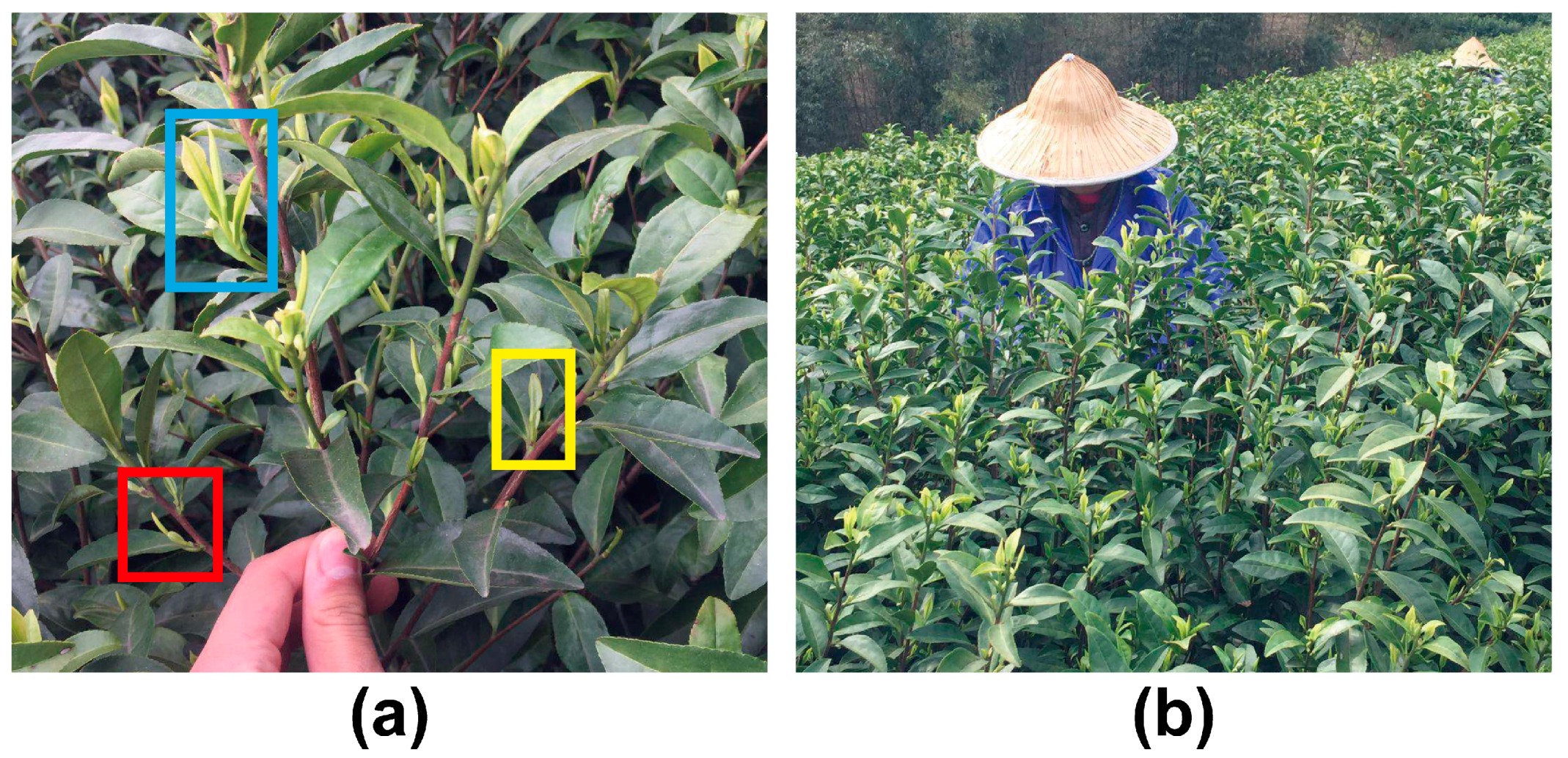
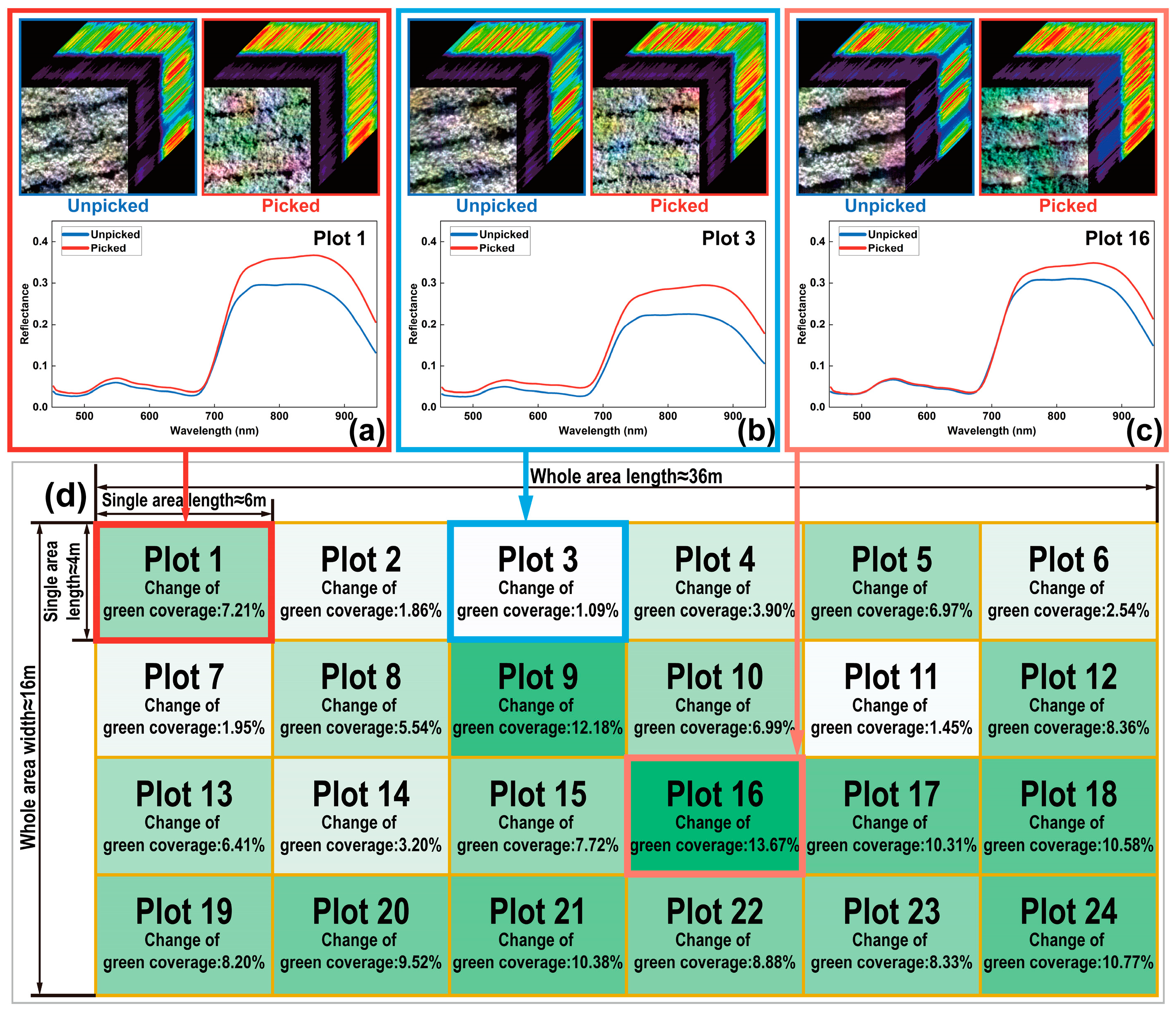
2.1.1. Research Subject and Test Plot Design

Anji white tea (Camellia sinensis cv. Baiye1), a typical planting variety of tea that is only produced in the spring [45,46], was selected as the research subject in this study. Its yield estimation has a practical application and can act as a significant reference for developing a yield estimation method for spring tea in general. Anji white tea was originally produced in Anji County at the northern foot of Tianmu Mountain in the northwest of Zhejiang Province, China [47]. The geographical range of Anji County is 30°23′~30°53′N, 119°14′–119°53′E. The climate and ecological conditions here are very favorable, and it has always been a famous, high-quality producing area for spring tea [48]. This study was conducted at Bauming Tea Garden in Anji County (see Figure 1). The altitude difference of the test area was less than 5 m a.s.l.
As the picked buds and young leaves comprise the components of the spring tea yield, the spectral difference in the picked and unpicked tea tree canopies is produced by picking these components. In this study, research on the relationship between the spectral index difference in unpicked and picked tea tree canopies and yield was performed. The 24 test plots (within a rectangle: about 4 m × 6 m) with markedly variable green coverage and a fresh yield were selected, and the test data from each plot, including the hyperspectral images of unpicked and picked tea tree canopies, the fresh weight of the tea yield, and the auxiliary data acquisition (near-ground photos of picked and unpicked canopies for measuring the green coverage change, the chlorophyll content of tea yield components, and mature leaves, and the tea yield component area), were collected from 4–6 April 2019.
Figure 1. Location of the test area.
Remotesensing 15 01100 g001

2.1.2. Hyperspectral Data Collection and Preprocessing

The DJI M600 UAV (Figure 2) was used as the flight platform, and the UHD-185 hyperspectral imager (Figure 2a) was equipped to obtain hyperspectral images (Figure 2b). The total weight of the sensor was 470 g, and hyperspectral images of 125 spectral channels from 450 to 950 nm were obtained.
The acquisition of hyperspectral data was done in sunny and windless weather. UHD-185 sensor is installed on the platform, the lens is vertically downward, and the flight altitude is 50 m. The spatial resolution of the hyperspectral image was around 2 cm per pixel. A black-and-white reference pan was used for reflectivity conversion and radiation correction, and the spectral quality of the spliced images was checked to ensure that it met the analysis requirements [49].
Since a single image cannot cover the whole test area, Agisoft Photoscan software was employed for splicing a hyperspectral 3D cube image of the test area [50]. The spliced UAV hyperspectral images from the unpicked and picked test areas are illustrated in the upper part of Figure 3. The noise from the soil and the other irrelevant images were contained in the spliced hyperspectral 3D cube image, and the removal of irrelevant information was performed with ENVI software [51]. The spectral characteristics of the unpicked and picked tea tree canopies of the whole test area are illustrated in the lower part of Figure 3.

2.1.3. Spring Tea Yield Data Collecting and Preprocessing

Spring tea picking is commonly carried out via the manual picking mode [52]. In this study, skilled tea pickers were employed for tea picking and for measuring the fresh yield. The picking action was performed for the selected 24 plots based on the standard picking patterns [29]: single bud, 1 leaf-1 bud, and 2 leaves-1 bud (see Figure 4). The fresh weights of the buds and young leaves were weighed using an electronic balance with a sensitivity of 0.01 g. In this paper, yield refers to the total amount of tea picked from tea trees. In 24 plots, the maximum weight of fresh tea was 879.570 g, the minimum was 153.870 g, the average was 483.863 g, and the standard deviation was 199.954 g.

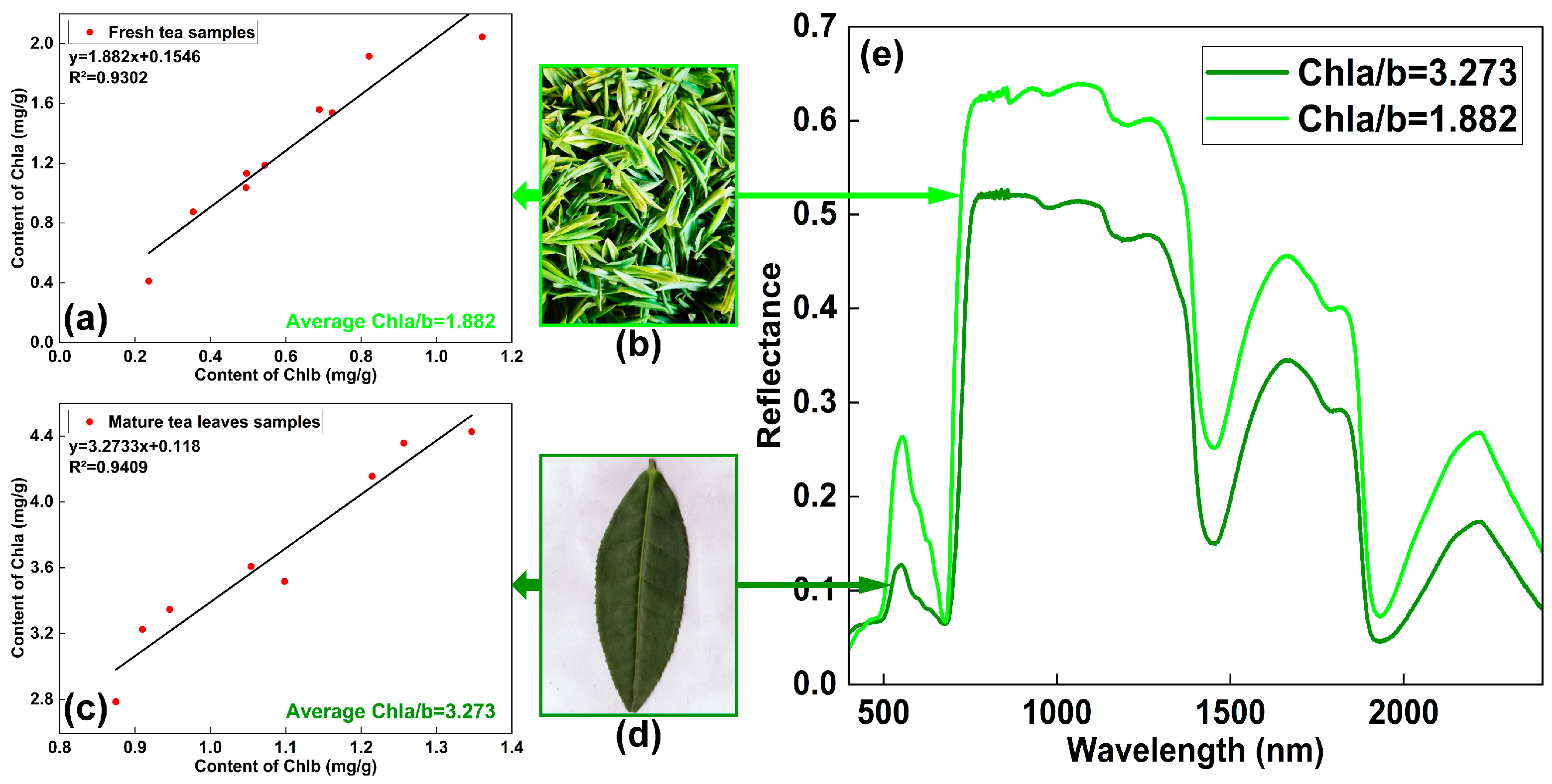
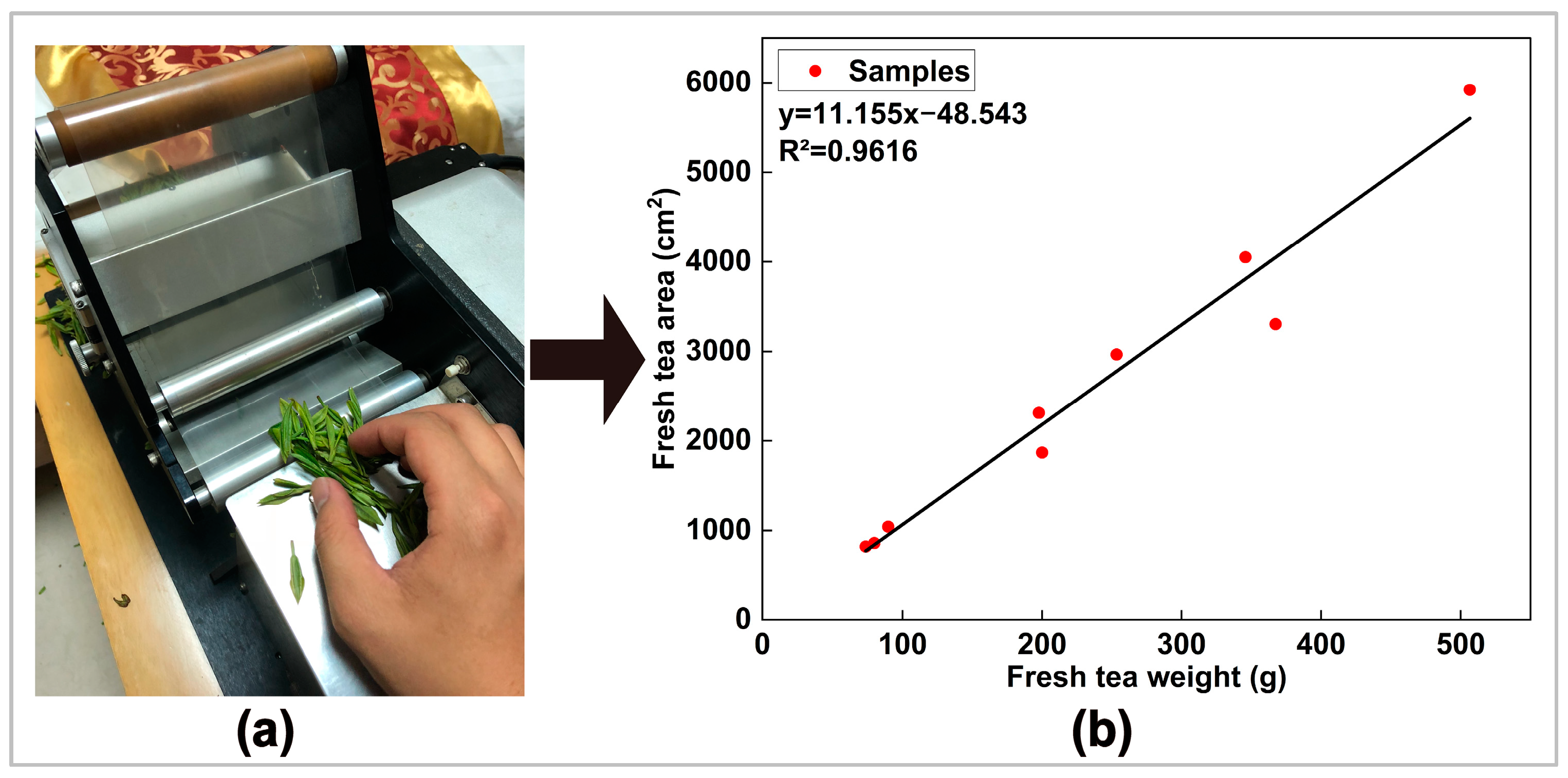
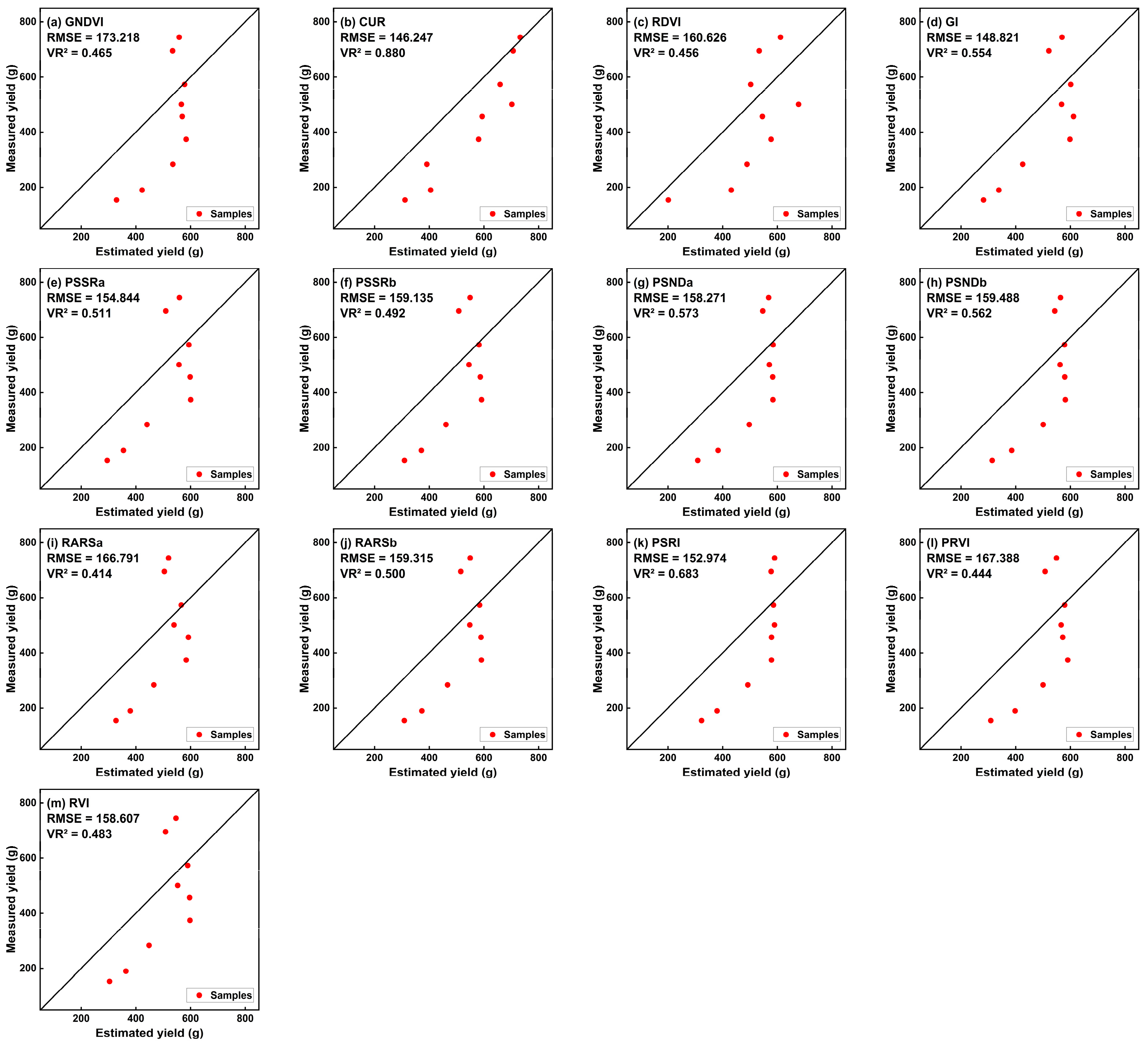
2.1.4. Auxiliary Data Acquisition

To help select the suitable vegetation index type for the spring tea yield estimation, we also collected auxiliary data, including the measurements of the chlorophyll a/b content ratio, the spectra of fresh tea (picked buds and young leaves), and the mature leaves from the tea tree canopy, as well as measurements of the fresh tea area, weight, and the green coverage change between the unpicked and picked tea tree canopies.
(1)
Chlorophyll ratio and spectra between fresh tea and mature leaf measurements
For the fresh tea yield estimation test, the buds and young leaves that comprise the fresh tea yield components, as well as the mature leaves, were collected from the Anji white tea tree canopy. Their chlorophyll a and b content were measured following the protocol reported by Hosgood et al. [53]. Their spectra in the range of 350–2500 nm were measured using the method reported for using the ASD FieldSpec 4 [54]. The results showed (see Figure 5): (1) There was a stable and obvious difference in the ratio of chlorophyll a (Chla) and chlorophyll b (Chlb) between the freshly picked tea components (Chla/Chlb = 1.882, Figure 5a) and the mature leaves (Chla/Chlb = 3.273, Figure 5), in which the mature leaf was the main responder to the tea tree canopy spectrum. (2) There was also an obvious spectral difference between the fresh tea components and the mature leaves from the tea tree canopy (Figure 5e), especially in the range of 550–690 nm, which is the chlorophyll absorption spectral region. This provided a basis for the spectral difference between the unpicked and picked spring tea canopies. Thus, chlorophyll spectral indices were employed to extract information on spring tea yield components and to conduct exploratory research on the yield estimation of spring tea with remote sensing data.
(2)
Area measurement/determination of fresh tea components
In this study, LI-3000A, a leaf area meter, was employed to measure the leaf area of the picked tea yield components (including the picked tea buds and young leaves). The measurement method followed the protocol reported by Delalieux [55]. The relationship between the measured area and the weight of the fresh tea components, which was a perfect linear correlation, is illustrated in Figure 6. The leaf area is the other important factor in the spectral response in the plant canopy. Thus, in this study, leaf area spectral indices (LASIs) were employed to conduct exploratory research on spring tea yield estimation using remote sensing data.
(3)
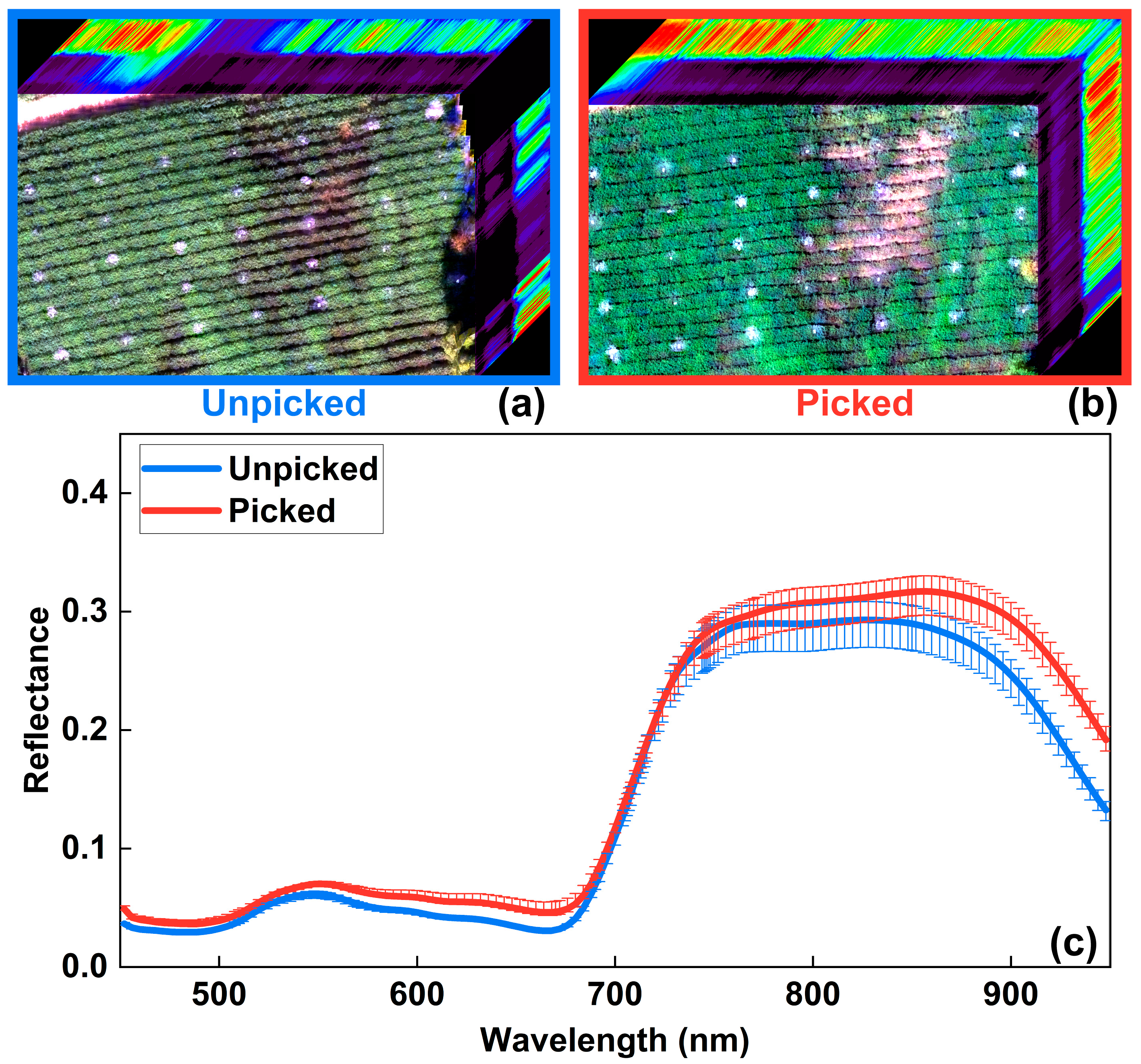
Green coverage change acquired via unpicked and picked tea tree canopy data
As the tea tree canopy in the spring-tea-picking stage had high coverage, piecewise linear models (PLMSVs and PLMCVs) were employed to avoid the saturation phenomenon, using CSIs or LASIs for extracting spectral characteristics in these high-coverage canopies. In this study, the spectral difference between the unpicked and picked tea tree canopies was produced by the picked fresh tea yield components, and these picked components were the producers of the green coverage change between these canopies. Moreover, the spectral difference was extracted using CSIs, or LASIs were regarded as the variables of the piecewise models. Thus, to avoid the saturation phenomenon, using CSIs or LASIs for fresh tea yield estimation, the green coverage change in the unpicked and picked tea tree canopies was defined as the piecewise reference basis for the piecewise linear models. Here, the green coverage change and the spectral difference in the unpicked and picked tea tree canopies are shown in Figure 7.
An industrial camera (iRAYPLE A7A20CU201) with 12 megapixels was used to take near-ground photos of the unpicked and picked tea tree canopies from each plot. When taking photos, the camera faced the tea tree canopy, and was kept 0.5 m away from the top of the canopy.
In this study, to better acquire the green coverage change that was only produced by the spring tea yield components, the HSI space was employed for the green coverage change calculation [56]. Therefore, RGB images from industrial cameras were converted into HSI images [57]. First, the saturation degree channel of the HSI space was used to obtain the threshold value to remove white noise from the photos taken of the tea tree canopy. Then, the HSI hue channel was used to obtain the threshold value according to the Maximum Between-Class Variance (Otus Method) [58], and morphological processing [59] was used to remove the non-green parts of the taken photos, such as soil, stems of tea trees, etc. The total number of pixels and the number of white pixels in the original image were calculated, and the ratio was obtained as the result, i.e., the green coverage was obtained. Finally, the green coverage change for each test plot was obtained from photos of the unpicked and picked tea tree canopies.
Figure 7. The green coverage change and spectral difference between the unpicked and picked tea tree canopies. (ac) hold the green coverage change: 13.67%, 1.09%, and 7.21%, respectively. (d) green coverage change in each test plot.
Remotesensing 15 01100 g007

2.2. Methods

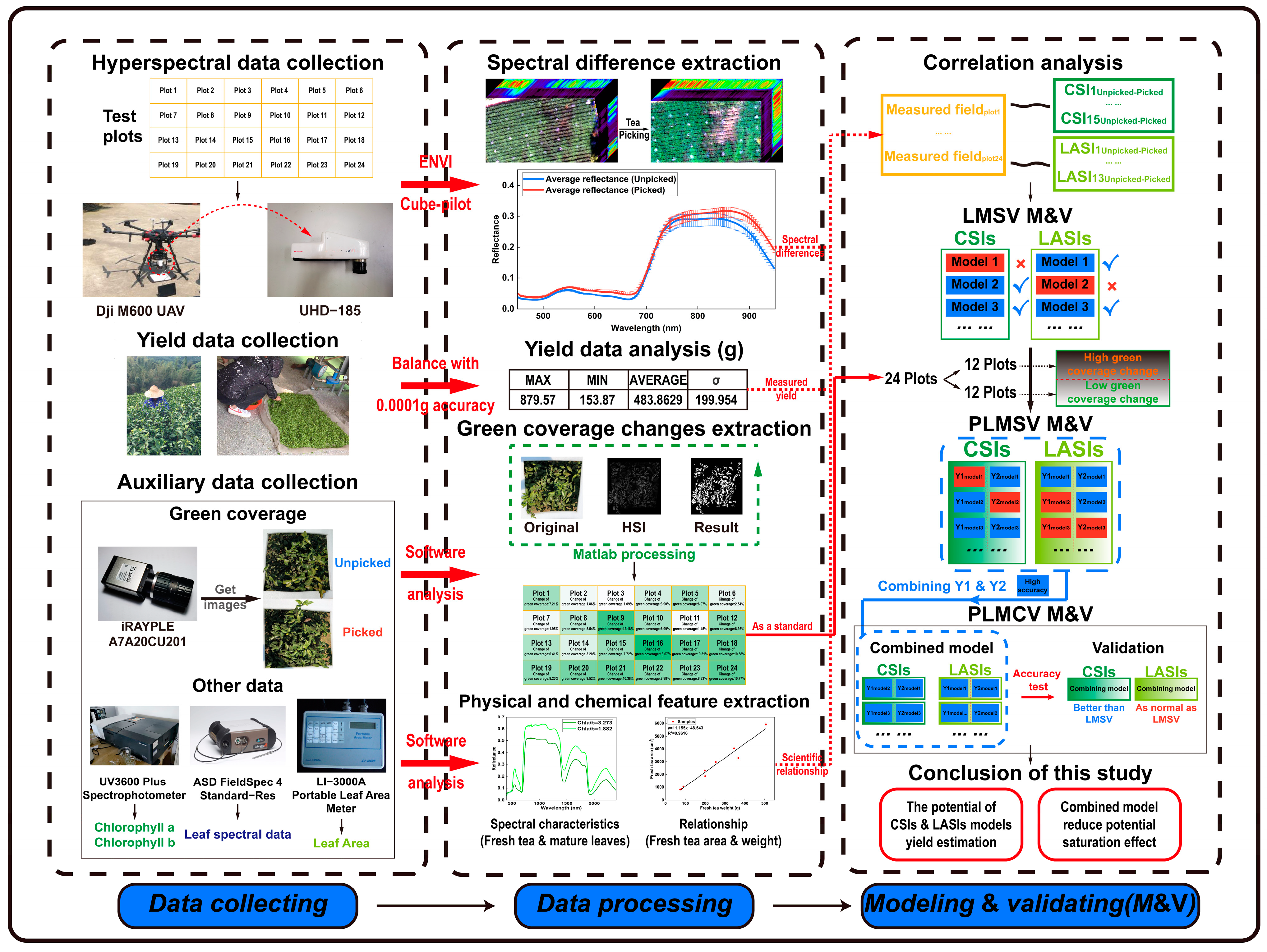
2.2.1. Research Technical Framework

This study was mainly divided into three steps (Figure 8). The first step was data collection, which included collecting the UAV hyperspectral data from the unpicked and picked tee tree canopies, the fresh tea yield for 24 test plots, and the auxiliary data. The second step was data processing, which included extracting the hyperspectral characteristics, analyzing the yield data, analyzing the chlorophyll a/b ratio, analyzing the spectral characteristics of the tea yield components and the mature leaves, and determining the green coverage change in the unpicked and picked test plots. The third step was modeling and validation, which included: (1) The selection of suitable chlorophyll spectral indices (CSIs) and leaf area spectral indices (LASIs) was performed via a correlation analysis of these collected vegetation indices. (2) The spring tea fresh yield estimation was determined using the linear model with a single index variable (LMSV), the piecewise linear model with the same index variables (PLMSV), and the piecewise linear model with the combined index variables (PLMCV). (3) The built models were verified and compared to evaluate the ability to estimate the spring tea fresh yield via UAV hyperspectral remote sensing.

2.2.2. Fresh Yield Estimation Method for Spring Tea by Heperspectral Remote Sensing Data

The research on the fresh yield estimation of spring tea consisted of vegetation index selection, LMSV modeling and validation, PLMSV modeling and validation, and PLMCV modeling and validation in which the PLMSVs and PLMCVs were considered the same.
(1)
Vegetation index selection for suitable spring tea fresh yield estimation
In this paper, 15 common CSIs and 13 common LASIs were collected to extract the hyperspectral characteristics of unpicked and picked tea tree canopies. The specific descriptions of the CSIs and LASIs are shown in Tables in Section 3.1. Here, some indices were used for extracting chlorophyll information, as well as for extracting leaf area information. We classified these indices as CSIs or LASIs. We classified these indices as CSIs or LASIs based on the classification of the published literature for extracting chlorophyll or leaf area information. The suitable CSIs and LASIs for spring tea fresh yield estimation were selected from the collected vegetation indices via a correlation analysis (see Formula (1)) of the difference in the CSIs and LASIs (dCSIs or dLASIs) of unpicked and picked tea tree canopy spectra and of their yield ( Y ) from all test plots.
ρ dVI , Y = Cov ( dVI , Y ) σ dVI , σ Y
where ρ dVI , Y is the correlation coefficient between dCSIs or dLASIs and Y ; Cov ( dVI , Y ) is the covariance between dCSIs or dLASIs and Y ; and σ dVI and σ Y are the standard deviations between dCSIs or dLASIs and Y from all test plots, respectively.
(2)
LMSV modeling and validation
A linear function with a single index variable (LMSV) was employed to establish the model of spring tea fresh yield estimation. In this study, there were sample data from 24 test plots for determining the spring tea fresh yield estimation, in which 15 sample data, including data on the difference in the CSIs or LASIs from the hyperspectral images of the unpicked and picked tea tree canopies and on the fresh tea yield from the corresponding test plots, were used to establish the model (Table in Section 3.2). The other 9 sample data were used for the validation of the established model.
The model determination coefficient ( MR 2 ) metric was employed for the evaluation of the established model, and a T-test was also employed to compare the difference between the MR 2 of these models and the CSIs or LASIs.
MR 2 = 1 i = 1 n ( Y mea i Y mod i ) 2 i = 1 n ( Y mea i Mean ( Y mea i ) ) 2
where MR 2 is the determination coefficient of the established model for fresh tea yield estimation in a linear function; n is the employed samples from the test plot data (n = 15); Y mea i is the i sample of the measured yield; and Y mod i is the modeled yield data in the corresponding sample.
The root-mean-square error (RMSE) and validation determination coefficient ( VR 2 ) metrics were employed for estimating the spring tea fresh yield. Additionally, a T-test was used to compare the difference between the RMSE and VR 2 .
RMSE = 1 m i = 1 m ( Y mea i Y est i ) 2 VR 2 = 1 i = 1 m ( Y mea i Y est i ) 2 i = 1 m ( Y mea i mean ( Y mea i ) ) 2
where Y est i is the yield estimation value of the model and m is the employed samples from the test plot data (m = 9) for the evaluation of the model.
(3)
PLMSV modeling and validation
The high coverage of the tea tree canopy could lead to saturation of the vegetation index during plant canopy spectral extraction. This problem can be solved by using a piecewise function [60,61] or by combining more vegetation indices when establishing the model [31]. In this study, the picked components of the spring tea yield produced a spectral difference between the unpicked and picked tea tree canopies. Thus, the green coverage change was used to establish a piecewise linear model with the same index variables (PLMSVs) for estimating the spring tea fresh yield with remote sensing data.
The piecewise standard was designed to be two segments, and the median (7.465%) of the green coverage change from the 24 test plots was used as the piecewise value. The piecewise function contained high (n = 12 samples) and low (n = 12 samples) green coverage change segments for the same single index (CSIs or LASIs). In the high segment, 6 samples were used for the establishment of the model, and the other 6 samples for the validation; in the low segment, the sample allocation method for the establishment and validation of the model was equally divided (6 and 6 samples). The evaluation metrics RMSE and VR2 were also applied for PLMSV validation.
(4)
PLMCV modeling and validation
As the saturation of the different vegetation indices for extracting plant canopy spectra was different [62], the piecewise linear model that combined different index variables (PLMCVs) was employed to better explore the saturation of CSIs or LASIs for the fresh yield estimation of spring tea.
In this study, the function (Y1) with a vegetation index (CSI or LASI) variable from PLMSV in the high green coverage change segment was combined with the function (Y2) with another vegetation index (CSI or LASI) variable from PLMSV in the low green coverage change segment (Figure 9). These combined piecewise linear functions were called PLMCV with the two combined vegetation index variables. As the different vegetation index held the different abilities of extracting spectra for fresh yield estimation of spring tea, the part of PLMCVs were selected and exhibited in this paper. The selection standards for CSI were PLMSVs with a VR2 over 0.45 and a low RMSE of 180 g from the different CSI, and the standards for LASIs were a better VR2 and RMSE from the different LASI. In addition, when the performances of PLMSV for the yield estimation in the high and low green coverage change segments were good, the functions (Y1 and Y2) were also combined with a PLMCV (Figure A5a and Figure A6a).
A comparison between the LMSV, PLMSVs, and PLMCVs was performed to explore the saturation of the spectral extraction with CSIs or LASIs in the fresh yield estimation of spring tea. To ensure the uniformity of the data, the data (n = 24 plot samples) for the LMSV validation were provided; 12 samples in the high green coverage change segment and 12 samples in the low green coverage change segment were provided for the PLMSV validation, and n = 24 plot samples were provided for PLMCV validation. The evaluation metrics RMSE and VR2 were used for the LMSV, PLMSVs, and PLMCVs.
Figure 9. Sketch map for the establishment method of PLMCV ((a-7) in this figure) from the linear functions of PLMSC. LMSV was for the linear model with a single index variable (a-1,a-4); PLMSV for the piecewise linear model with the same index variable; PLMCV for the piecewise linear model with the combined index variable; H for PLMSV in the high green coverage change segment; L for PLMSV in the low green coverage change segment; selected for the selected functions from PLMSV (red dashed boxes (a-2,a-6) for PLMCV. Unselected for the unselected functions for PLMCV (a-3,a-5).
Remotesensing 15 01100 g009

3. Results and Analysis

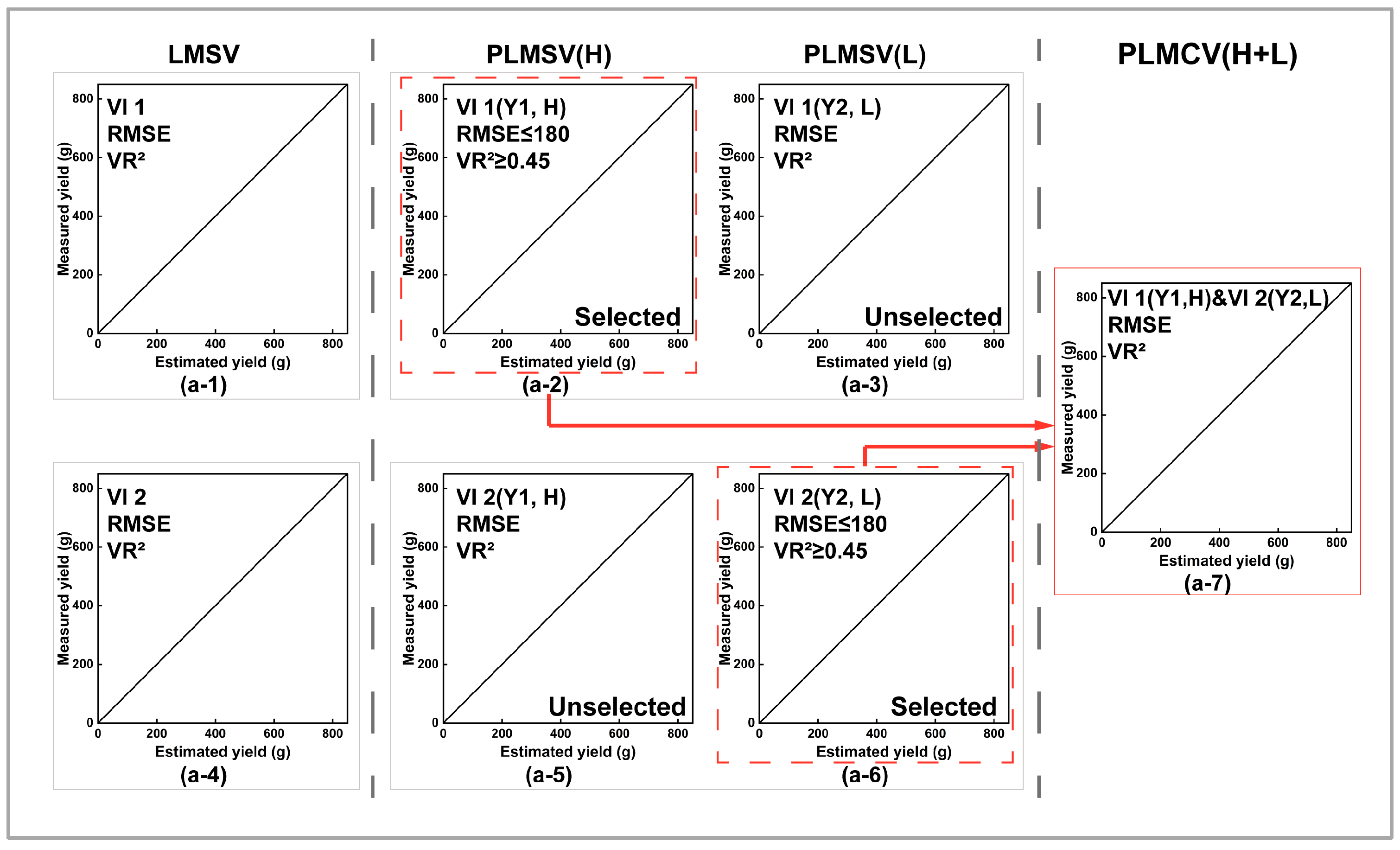
3.1. Vegetation Index Selection for Suitable Spring Tea Fresh Yield Estimation

To obtain information on vegetation biophysical parameters by using remote sensing data, the employed vegetation indices should maximize sensitivity to plant biophysical parameters well with a linear response in order that sensitivity is available for a wide range of vegetation conditions, facilitating validation and calibration of the index [63]. In this study, the selection standards of the employed indices from the collected CSIs or LASIs for the estimation of the spring tea fresh yield were a linear correlation coefficient over 0.5, and a significance test at the 0.05 level (See Table 1 and Table 2).
In the collected 15 chlorophyll spectral indices (CSIs) and 13 leaf area spectral indices (LASIs), the correlation between the difference in the CSIs (dCSIs) from unpicked and picked tea tree canopies and their yields from all test plots (see Table 1) was better than that between the difference in the LASIs (dLASIs) and the yields (see Table 2) as a whole. According to the selection standards of a linear correlation coefficient over 0.5 and a significance test at the 0.05 level, 13 CSIs were selected to build the yield estimation model from the 15 collected CSIs. The LASIs selected for the yield model were the NDVI, TVI, MCARI1, MCARI2, R750/R710 and D715/D705. These selected CSIs or LASIs were used to build the spring tea fresh yield estimation model with a linear function.

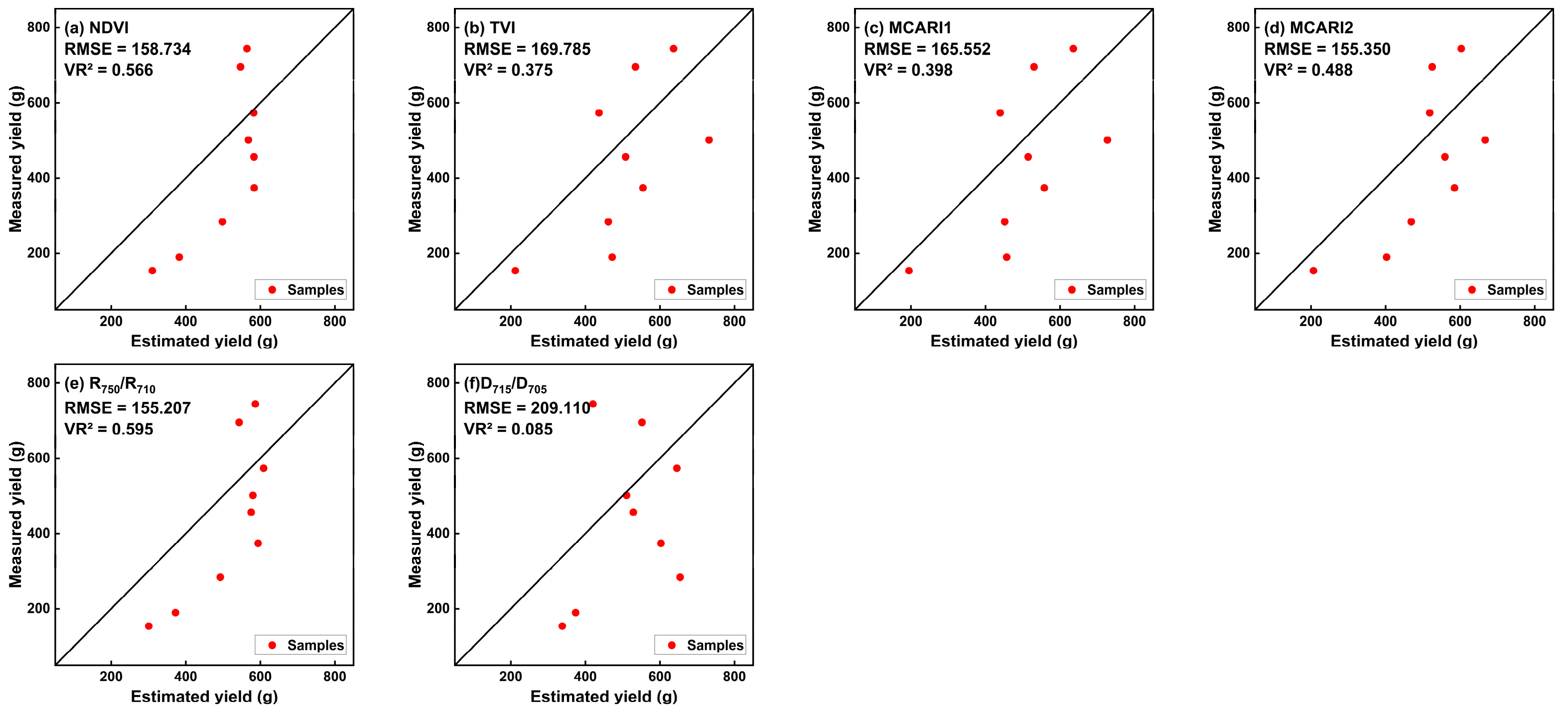
3.2. LMSV Establishment and Validation for Spring Tea Fresh Yield Estimation

In the single vegetation index model with a linear function (the linear model with the single index variable (LMSV)), the MR2 metrics of the estimation model of the spring tea fresh yield were all over the 0.05 significance test level for the selected CSIs and LASIs (Table 3), in which the CUR, RDVI, GI, and PSSRa from the selected CSIs and the TVI, MCARI1, MCARI2, and R750/R710 from the selected LASIs were over the 0.01 significance test level. As a whole, the performance of the selected CSI was better than that of the selected LASI for establishing the spring tea fresh yield estimation model with a linear function. The best performance of these modeling functions was from the CUR, with an encouraging MR2 (0.611) and a 0.01 significance test level.
For the ability of the LMSV, the VR2 metrics of the estimation model from the selected CSI, except for that of the RARSa, were also over the 0.05 significance test level, but only the corresponding VR2 metrics of the NDVI, MCARI2, and R750/R710 from the selected LASI (Table 3, Appendix A) were over the 0.05 significance test level. The metrics (RMSE) of these models for the estimation of the spring tea yield were lower than 160 g from the selected CSIs, but only those from the NDVI, MCARI2, and R750/R710 were lower than 160 g from the selected LASIs.
In Table 3, an inconsistency was found between the evaluation metrics of MR2 for modeling and VR2 and RMSE for validation with regard to the single vegetation index. For example, for the RDVI, its MR2 was over 0.5 and was at a 0.01 significance test level, but its VR2 was lower than 0.5 and was at a 0.05 significance test level, and its RMSE was higher than 160 g. This could be due to the tea tree canopy in the spring-tea-picking stage having high coverage, causing these indices to display saturation during the plant canopy spectral extraction.

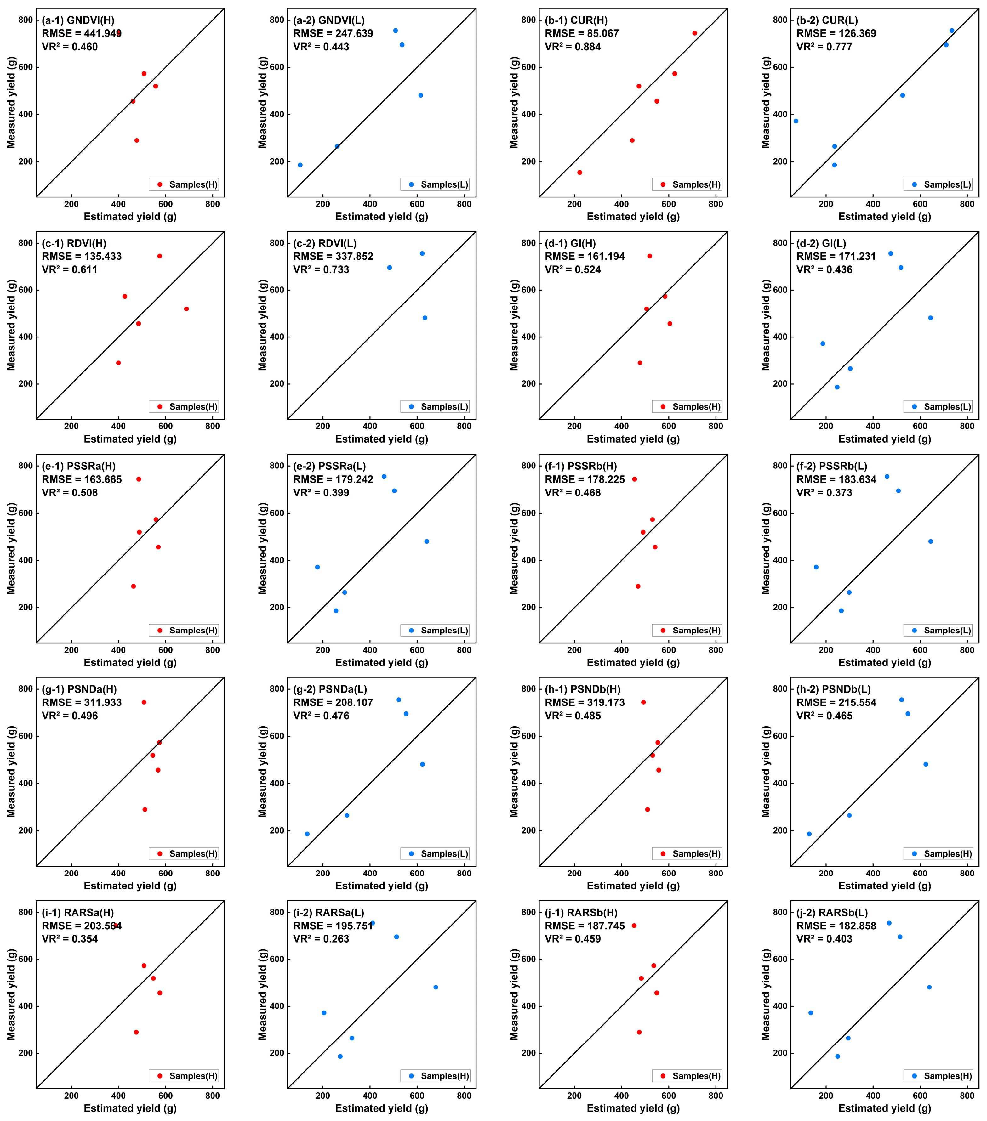
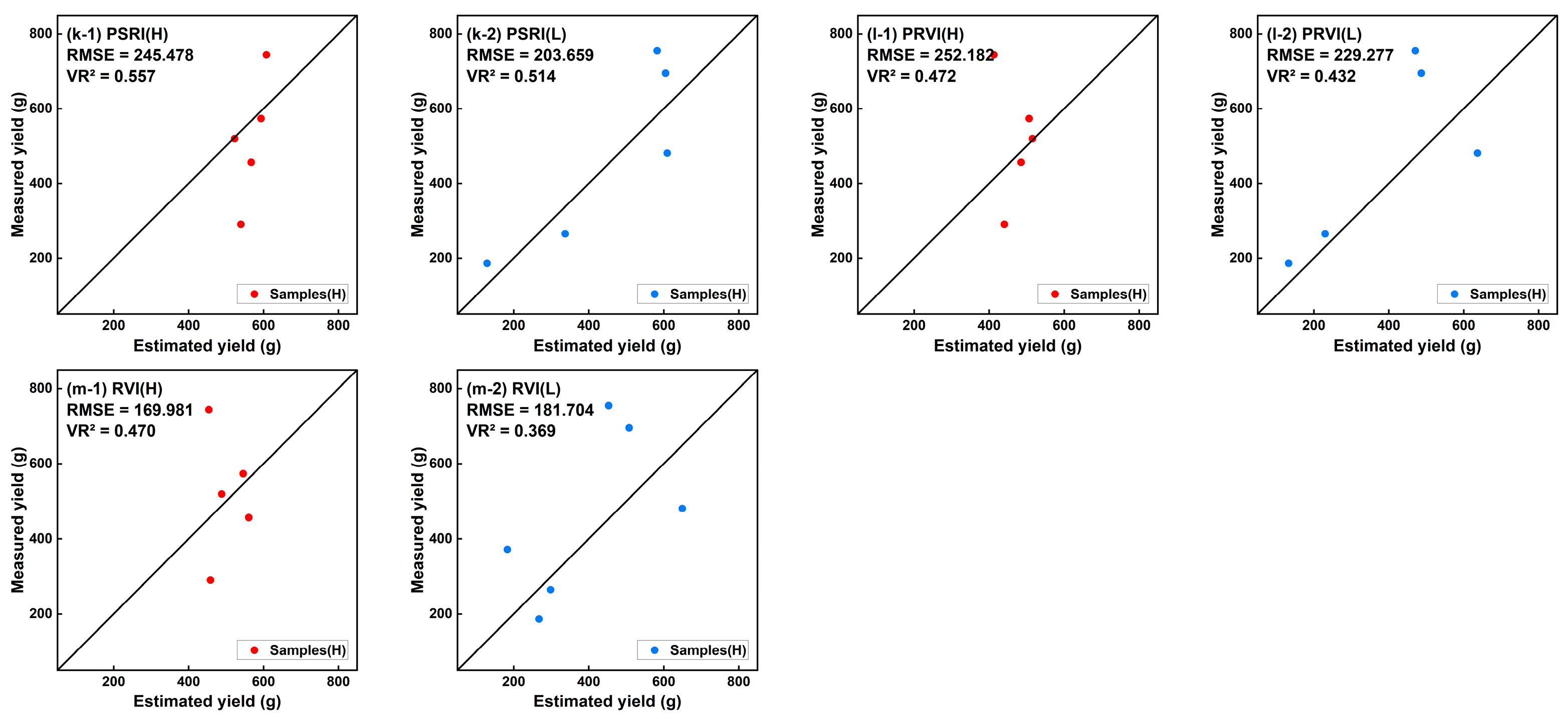
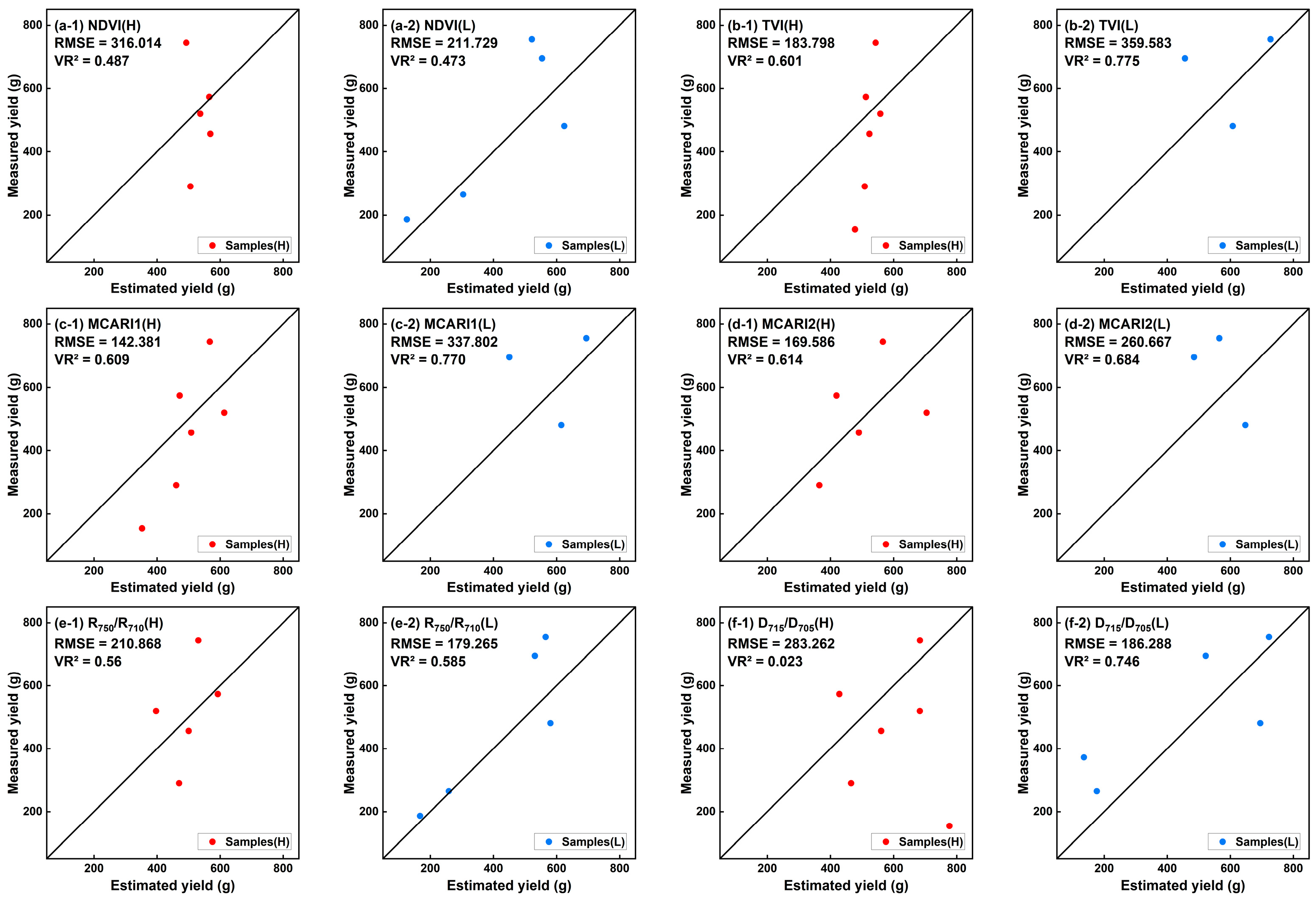
3.3. PLMSV Establishment and Validation for Spring Tea Fresh Yield Estimation

The performance of the establishment and validation of the spring tea fresh yield piecewise linear model with the same index variables (PLMSVs) is shown in Table 4 and Appendix B. In the high green coverage change model, the validation accuracy of the yield model based on the CUR was the highest, and the RMSE was as low as 85.067 g. The models (Y1) based on the GI, PSSRa, PSSRb, RVI, MCARI1, and MCARI2 had good validation accuracy, with an encouraging VR2 and RMSE that was lower than or approximate to 160 g. In the low green coverage change model, the validation accuracy of the yield model based on the CUR was also the highest, and the RMSE was as low as 126.369 g. The models (Y2) based on the GI, RVI, R750/R710 and D715/D705 had good validation accuracy with an encouraging VR2 and RMSE that was lower than or approximate to 180 g.
Compared to the LMSV, the range in the MR2, RMSE and VR2 of PLMSVs from the selected CSIs and LASIs were all amplified by the piecewise function. The estimation ability of the model based on the CUR was obviously improved in the high and low green coverage changes seen in the tea tree canopy. This result shows that the sensitivities of the selected CSIs to fresh tea yield models improved, and the saturation of these vegetation indices due to the high coverage of the spring tea tree canopy was reduced.
Table 4. PLMSV establishment and validation for spring tea yield estimation. Y1 was for a yield estimation in the segment of high green coverage change (H) from the unpicked and picked tea tree canopies, and Y2 was for a model in the low green coverage change (L).
TypedVIModeling (n = 12)Validation (m = 12)
Yield Estimation ModelM-R2RMSE (g)V-R2
dCSIGNDVIY1 = −32,856dVI − 68.3670.788 **441.9490.460
Y2 = −12,356dVI + 409.490.452247.6390.443
CURY1 = −10,275dVI − 257.670.39485.0670.884 ***
Y2 = −10,704dVI − 266.590.567 *126.3690.777 **
RDVIY1 = −9228.1dVI + 154.70.166135.4330.611 *
Y2 = −15,582dVI − 48.0190.724 **337.8520.733 **
GIY1 = −1372.9dVI + 425.160.656 **161.1940.524 *
Y2 = −846.11dVI + 520.870.551 *171.2310.436
PSSRaY1 = −206.55dVI + 328.40.73 **163.6650.508 *
Y2 = −126.42dVI + 471.250.519 *179.2420.399
PSSRbY1 = −270.69dVI + 438.660.74 **178.2250.468
Y2 = −163.05dVI + 555.570.479183.6340.373
PSNDaY1 = −9862.2dVI + 366.510.635 **311.9330.496
Y2 = −4258.5dVI + 529.340.554 *208.1070.476
PSNDbY1 = −11,273dVI + 479.930.657 **319.1730.485
Y2 = −4813.9dVI + 579.560.555 *215.5540.465
RARSaY1 = −1001.3dVI + 811.070.677 **203.5640.354
Y2 = −605.13dVI + 792.270.404195.7510.263
RARSbY1 = −342.43dVI + 399.320.718 **187.7450.459
Y2 = −200.47dVI + 532.140.488182.8580.403
PSRIY1 = 19,446dVI + 403.790.464245.4780.557 *
Y2 = 9270.7dVI + 529.210.602 *203.6590.514 *
PRVIY1 = −1201.6dVI − 35.50.775 **252.1820.472
Y2 = −684.55dVI + 305.650.499229.2770.432
RVIY1 = −198.29dVI + 402.670.743 **169.9810.470
Y2 = −123.63dVI + 526.680.482181.7040.369
dLASINDVIY1 = −10,003dVI + 451.510.645 **316.0140.487
Y2 = −4312.8dVI + 566.440.555 *211.7290.473
TVIY1 = −22.706dVI + 481.470.005183.7980.601 *
Y2 = −383.43dVI − 320.90.717 **359.5830.775 **
MCARI1Y1 = −2692.6dVI + 343.050.047142.3810.609 *
Y2 = −12,929dVI − 380.410.755 **337.8020.770 **
MCARI2Y1 = −6573.7dVI + 112.360.325169.5860.614 *
Y2 = −7170.4dVI + 137.650.69 **260.6670.684 **
R750/R710Y1 = −4439.1dVI − 187.190.681 **210.8680.560 *
Y2 = −2293.6dVI + 222.190.593 *179.2650.585 *
D715/D705Y1 = 6982.1dVI + 272.990.103283.2620.023
Y2 = −10,886dVI + 929.840.587 *186.2880.746 *
Note: *** Significant at the 0.01 level; ** Significant at the 0.05 level; * Significant at the 0.1 level.

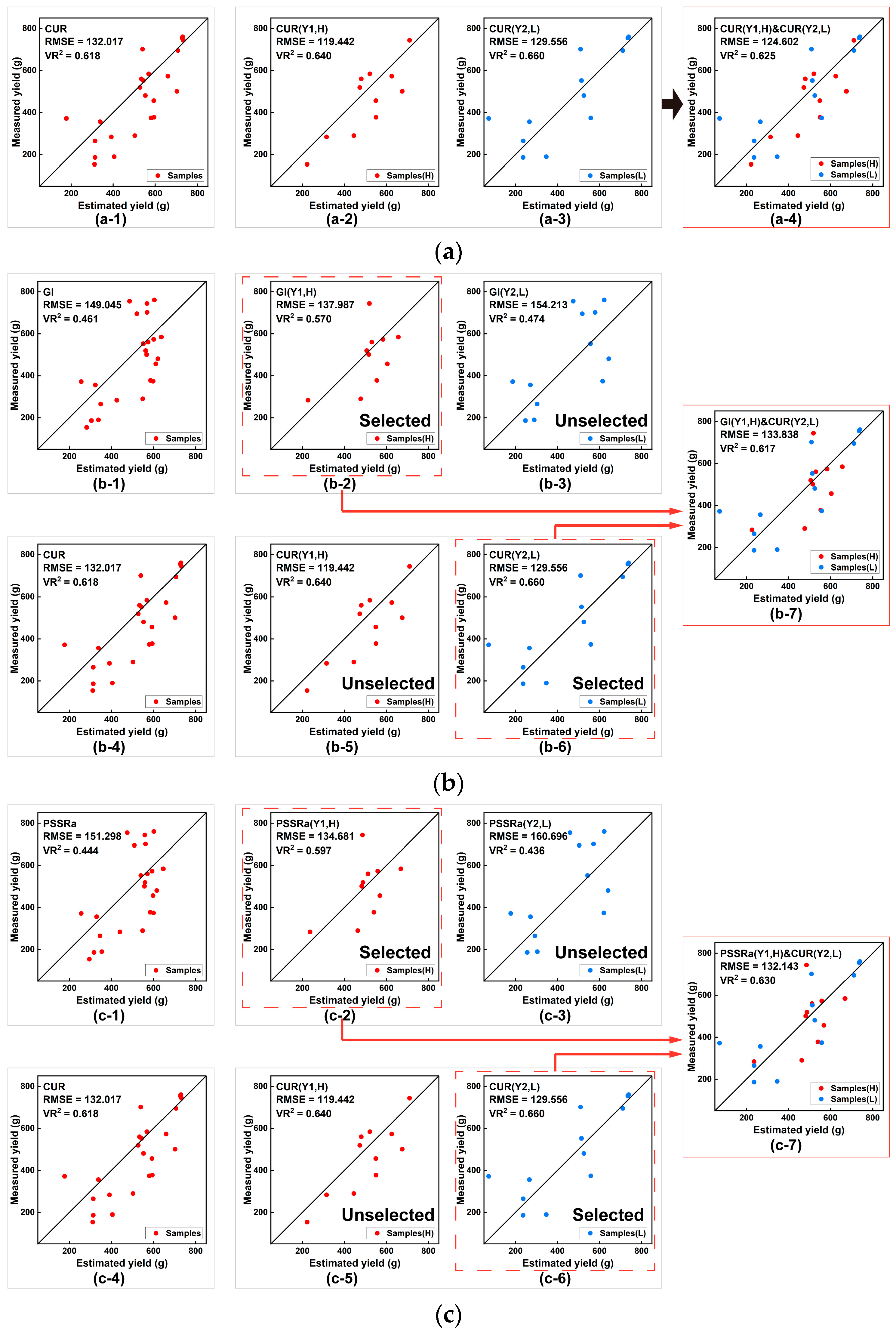
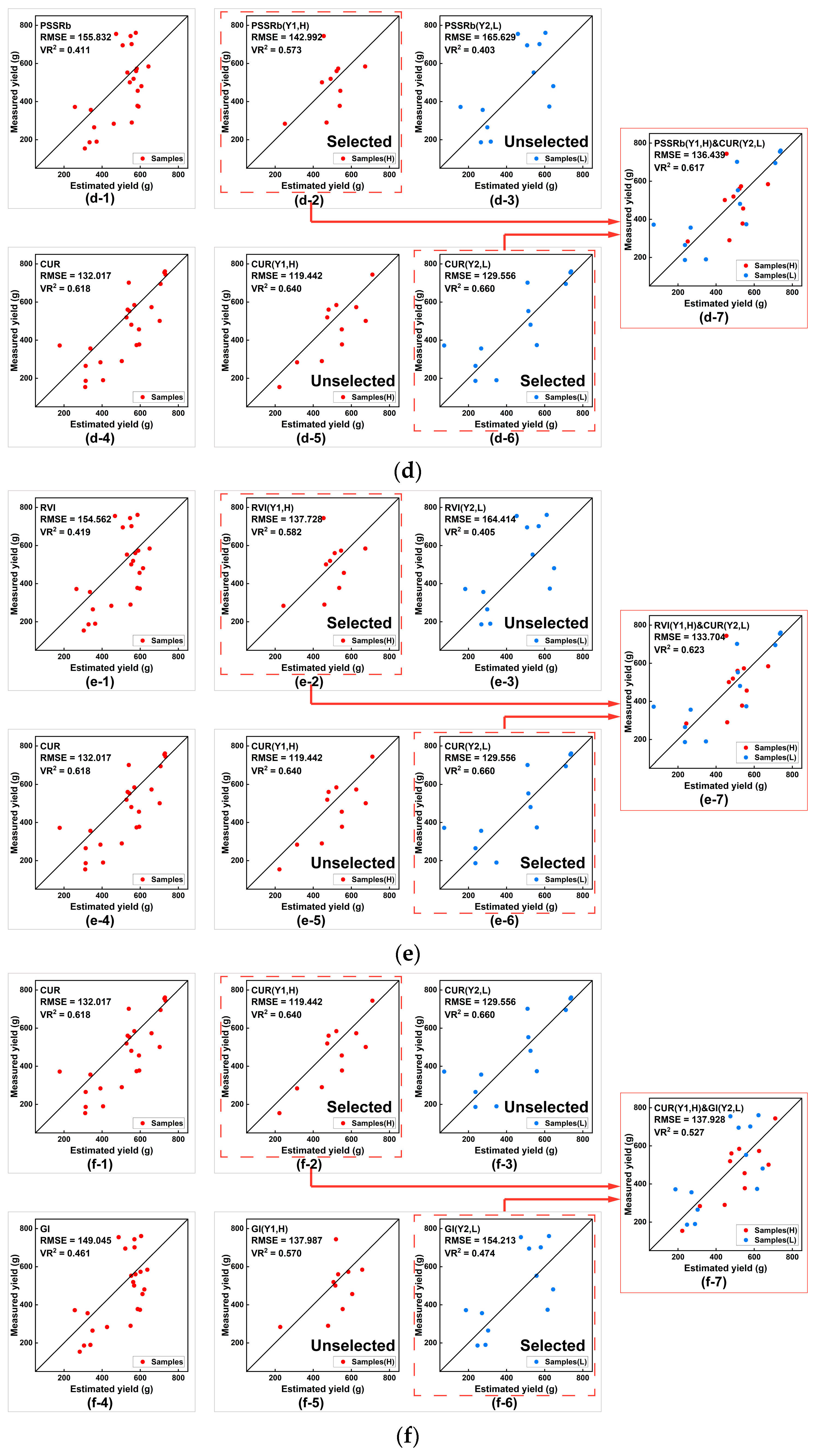
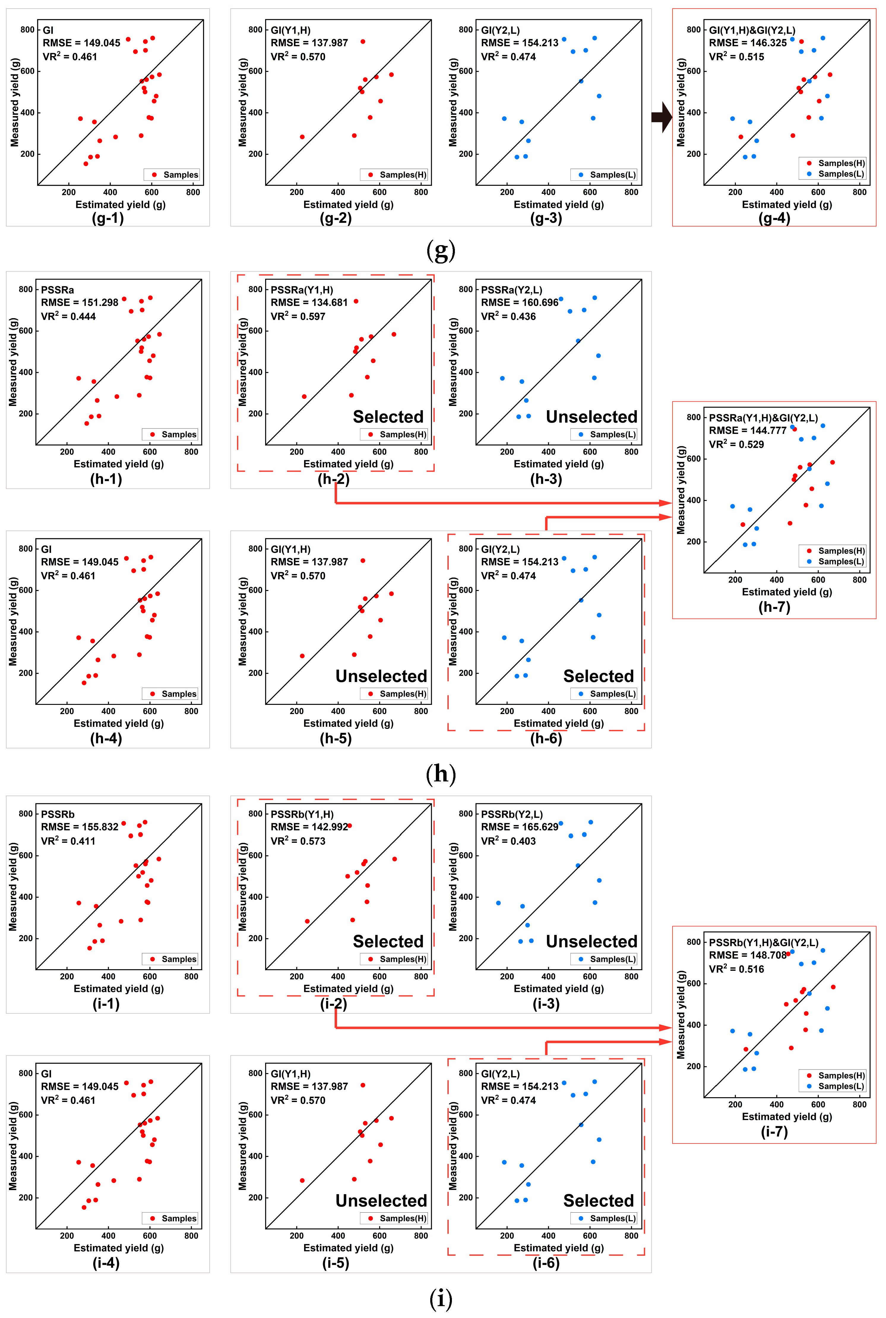
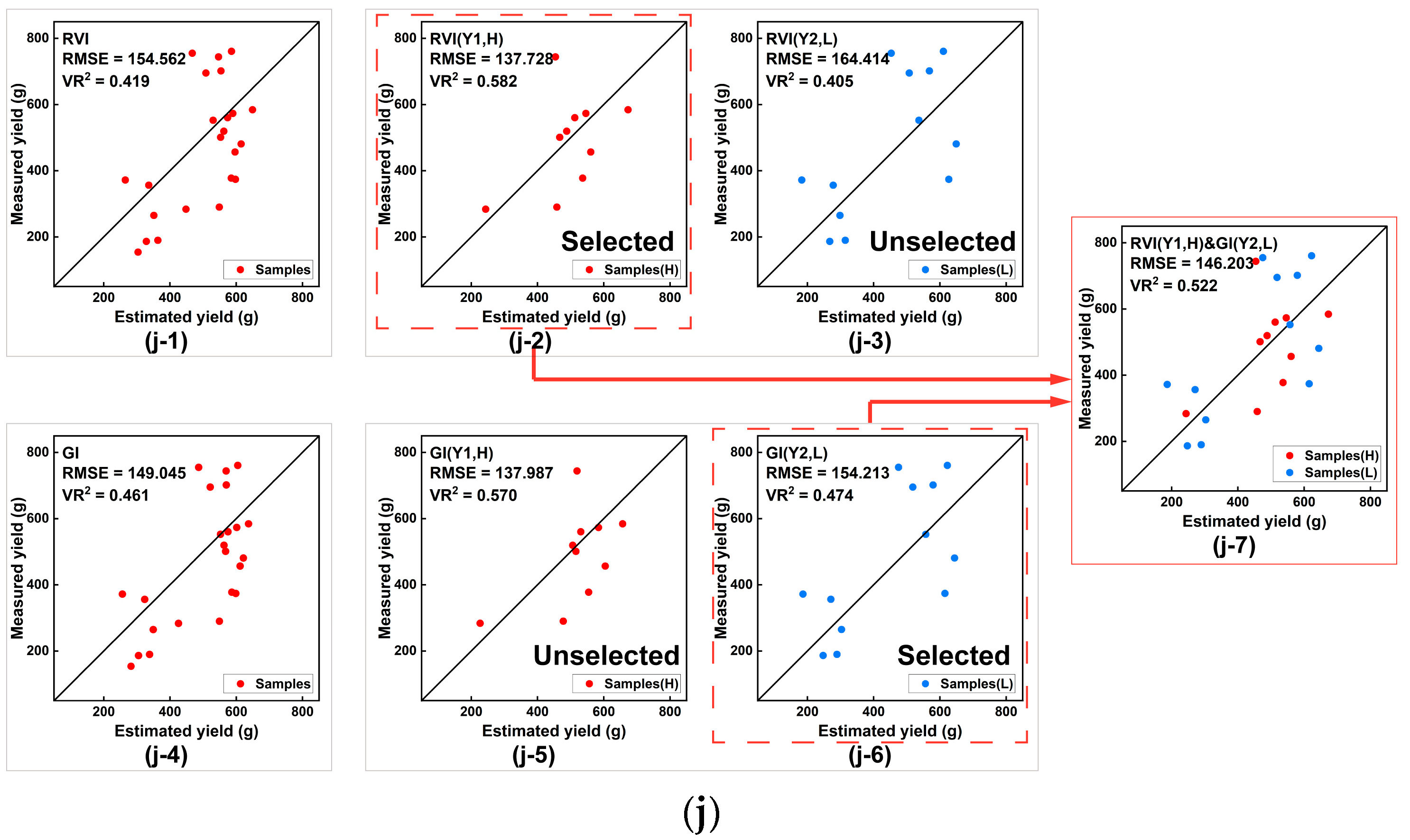
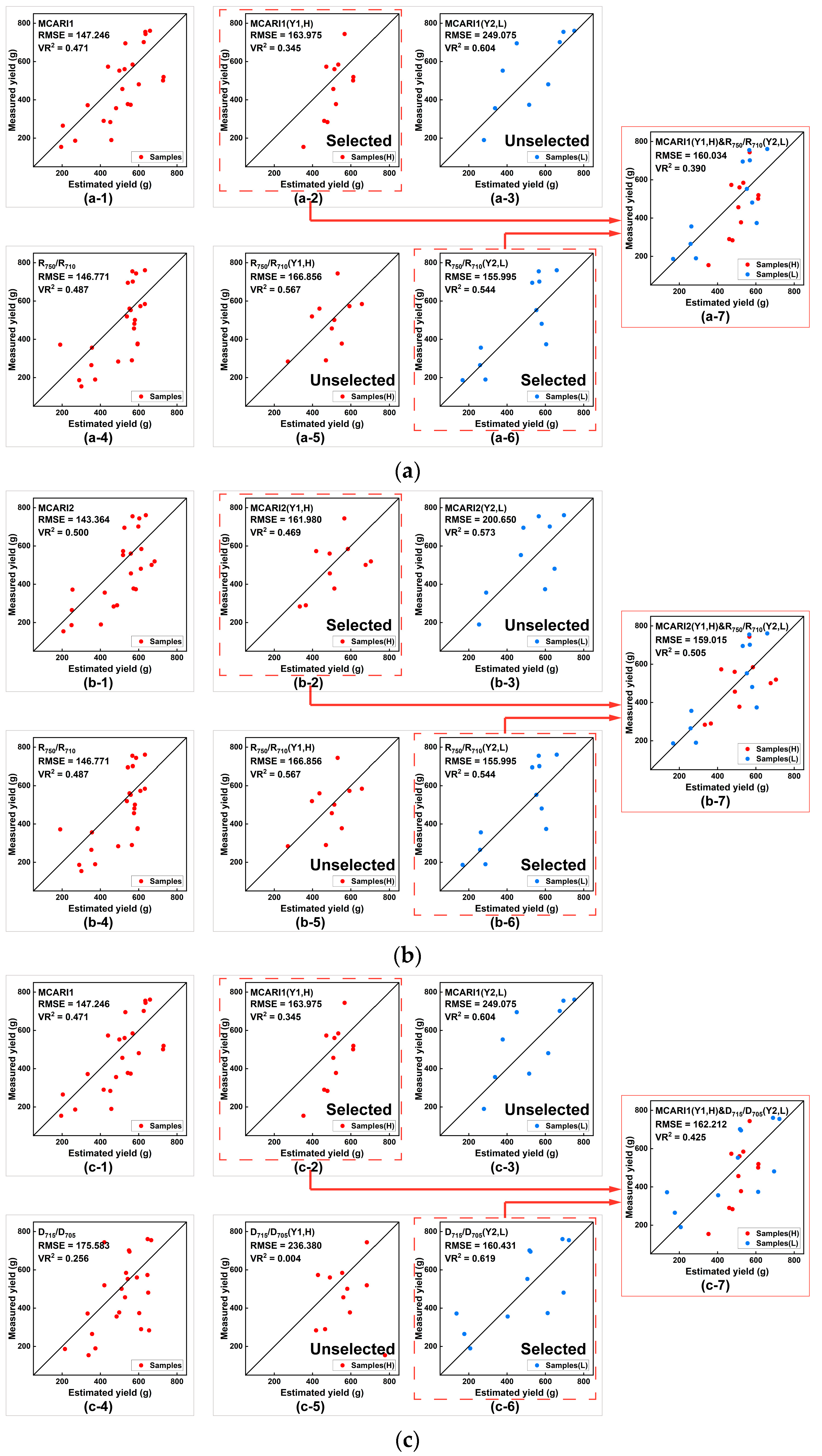
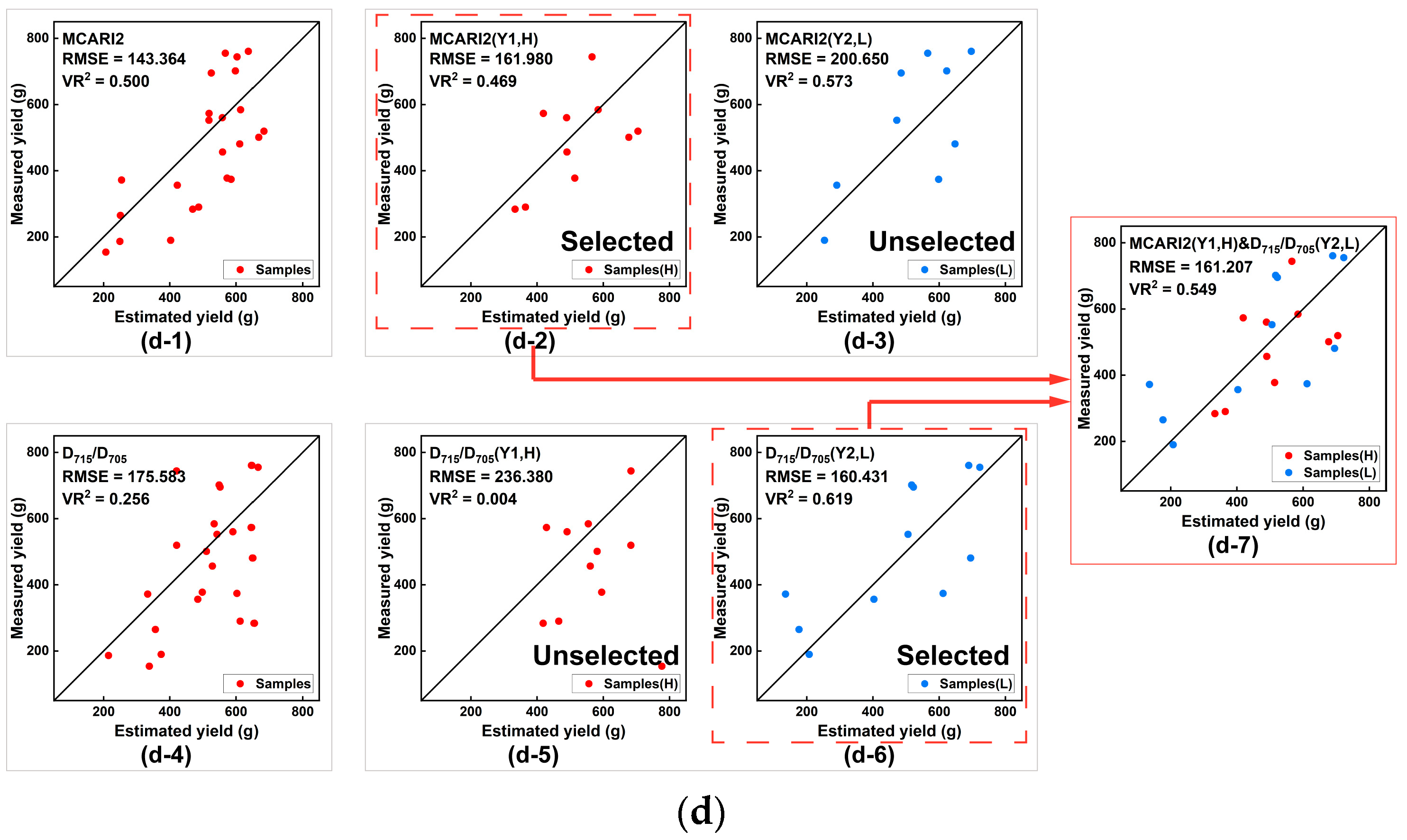
3.4. PLMCV Validation for Spring Tea Fresh Yield Estimation

To explore the action of combining indices and their effect on reducing the saturation of the spring tea yield estimation in the high coverage tea tree canopy, PLMCVs were evaluated, and the results are displayed in Table 5. For the SCIs, the models (Y1) based on the CUR, GI, PSSRa, PSSRb, and RVI for the low green coverage change segment and the models (Y2) based on the CUR and GI were selected due to their encouraging VR2 and RMSE metrics (see Table 4) for building the combined models of spring tea fresh yield estimation. Additionally, 10 combined models were built based on SCIs. For the LASIs, the models (Y1) based on MCARI1 and MCARI2 for the low green coverage change segment and the models (Y2) based on the R750/R710 and D715/D705 were selected, and four combined models were built. Moreover, comparisons of the estimation ability of the linear model, the piecewise linear model, and the combined model were performed in which 24 samples from all test plots were used for the model evaluation.
Compared with the LMSV, the RMES and VR2 metrics of the combined model from the CSIs in PLMCVs were all improved in these five combinations of indices: CUR (Y1,H) and CUR (Y2,L), GI (Y1,H) and GI (Y2,L), PSSRa (Y1,H) and GI (Y2,L), PSSRb (Y1,H) and GI (Y2,L), and RVI (Y1,H) and GI (Y2,L); the other five combinations did not show improvements. Here, the best performance of a combined model was CUR (Y1,H) and CUR (Y2,L), as it had an encouraging RMSE (124.602 g) and VR2 (0.625). However, the RMSE metrics of the combined model based on the LASIs were reduced. The results showed that the model based on the CSIs for spring tea fresh yield estimation could be improved with PLMCVs but that the model based on the LASIs could not. This could be due to the fact that for CSIs, the chlorophyll a/b ratio and spectral characteristics of spring tea fresh yield components were different from those of the mature leaves from the tea tree canopy, but for LASIs, the area of the components (buds and young leaves) of the fresh tea yield in spring was small compared with the area of the tea tree canopy.
Table 5. PLMCV establishment and validation for spring tea yield estimation. Y1 was for a yield estimation in the segment of high green coverage change (H) from the unpicked and picked tea tree canopies, and Y2 was for a model in the low green coverage change (L).
Index
Type
dVILMSV
(m = 24)
PLMSV
(Y1,H, n = 12)
PLMSV
(Y2, L, n = 12)
PLMCV
Y1 (H)&Y2 (L) (m = 24)
RMSEVR2RMSEVR2
CSICUR132.0170.618 ***Y1 = −10,275dVI − 257.67124.6020.625 ***
CUR132.0170.618 ***Y2 = −10,704dVI − 266.59
GI149.0450.461 ***Y1 = −1372.9dVI + 425.16133.8380.617 ***
CUR132.0170.618 ***Y2 = −10,704dVI − 266.59
PSSRa151.2980.444 ***Y1 = −206.55dVI + 328.4132.1430.630 ***
CUR132.0170.618 ***Y2 = −10,704dVI − 266.59
PSSRb155.8320.411 ***Y1 = −270.69dVI + 438.66136.4390.617 ***
CUR132.0170.618 ***Y2 = −10,704dVI − 266.59
RVI154.5620.419 ***Y1 = −198.29dVI + 402.67133.7040.623 ***
CUR132.0170.618 ***Y2 = −10,704dVI − 266.59
CUR132.0170.618 ***Y1 = −10,275dVI − 257.67137.9280.527 ***
GI149.0450.461 ***Y2 = −846.11dVI + 520.87
GI149.0450.461 ***Y1 = −1372.9dVI + 425.16146.3250.515 ***
GI149.0450.461 ***Y2 = −846.11dVI + 520.87
PSSRa151.2980.444 ***Y1 = −206.55dVI + 328.4144.7770.529 ***
GI149.0450.461 ***Y2 = −846.11dVI + 520.87
PSSRb155.8320.411 ***Y1 = −270.69dVI + 438.66148.7080.516 ***
GI149.0450.461 ***Y2 = −846.11dVI + 520.87
RVI154.5620.419 ***Y1 = −198.29dVI + 402.67146.2030.522 ***
GI149.0450.461 ***Y2 = −846.11dVI + 520.87
LASIMCARI1147.2460.471 ***Y1 = −2692.6dVI + 343.05160.0340.390 ***
R750/R710146.7710.487 ***Y2 = −2293.6dVI + 222.19
MCARI2143.3640.500 ***Y1 = −6573.7dVI + 112.36159.0150.505 ***
R750/R710146.7710.487 ***Y2 = −2293.6dVI + 222.19
MCARI1147.2460.471 ***Y1 = −2692.6dVI + 343.05162.2120.425 ***
D715/D705175.5830.256 **Y2 = −10,886dVI + 929.84
MCARI2143.3640.500 ***Y1 = −6573.7dVI + 112.36161.2070.549 ***
D715/D705175.5830.256 **Y2 = −10,886dVI + 929.84
Note: the script ‘—’ was for non-applying in PLMCV. *** Significant at the 0.01 level; ** Significant at the 0.05 level.

4. Discussion

4.1. Spectral Difference for Spring Tea Fresh Yield Estimation

Spectral monitoring/detection was greatly dependent on the spectral response of the observed objective at the specific wavelength [84], and these spectral characteristics are controlled by the spectral features of the matter and its light interception area of the monitoring objective [25]. In extracting spectral characteristics for spring tea yield estimation, the spectrum response factors of spring tea tree canopy at 450–950 nm were mainly chlorophyll spectral properties (Figure 3 and Figure 9) and leaf area in the tea tree canopy and its canopy structure. Moreover, the vegetation index could avoid the effect of canopy structure on spectrum extraction in plant information monitoring. Thus, the spectral response factors from the extraction with vegetation index in the tea tree canopy still contained the chlorophyll spectrum and leaf area information. In this study, the picked components (buds and young leaves) of the spring tea fresh yield were monitored with the spectral difference between the unpicked and picked tea tree canopies. The CSIs or LASIs differences from the unpicked and picked tea tree canopy spectra were employed to develop the fresh yield estimation model of spring tea. It was found that the performances of CSIs for spring tea fresh yield estimation were better than those of LASIs. This might be due to the small proportion of the light interception area for spring tea yield components in the tea trees, and to the low response to the spectral difference between the unpicked and picked tea tree canopies (Figure 4). Although most LASIs for monitoring vegetation information were proposed based on the chlorophyll spectral characteristics [85,86] and based on a study by Xing et al. [87], who proposed a single vegetation index for simultaneously monitoring the canopy chlorophyll density (CCD) and leaf area spectral index (LASI) of winter wheat, the LASIs had a weak performance when monitoring the small objective. For the CSIs, the obvious difference between the fresh tea yield components and the mature leaves in the canopy (Figure 5) was determined by using the spectral difference in the unpicked and picked tea tree canopy spectrum, in which the spectral difference method might reduce the effect of the canopy background, including that of the mature leaves and other factors. Thus, the CSIs for spring tea fresh yield estimation were ideal indices for spectral extraction on the basis of considering the spectral difference between the unpicked and picked tea tree canopies.

4.2. Reducing Saturation of Vegetation Index in High Coverage at Tea Tree Canopy

Tea tree canopy during the picking stage of spring tea has a high level of coverage, which can easily lead to spectral index saturation when extracting plant canopy spectra. In this study, PLMSVs or PLMCVs were designed to explore how saturation affects the performance of extracting the spectrum of spring tea fresh yield with CSIs and LASIs. The results showed that (1) PLMSVs from the selected CSIs and LASIs could improve the performance of the model determining the spring tea fresh yield (Table 5 and Figure A5a,h); (2) PLMCVs from the selected CSIs could also improve the performance, but the combination of indices from the selected LASIs could mostly did not improve the performance. This also shows that LASIs for spring tea fresh yield estimation had a weak performance from another perspective. Thus, it is necessary to consider saturation when extracting spectra with a vegetation index from a high-coverage plant canopy, especially when relying on chlorophyll information.
The research results from using the NDVI and RVI to determine the vegetation index saturations were the most reported for extracting the vegetation canopy spectrum [46,48]. In this study, by using PLMSVs, the performance of the model based on the NDVI did not improve the performance with regard to yield estimation accuracy, whereas the RVI model had a better performance (Table 5 and Figure A5e,j). This could be due to the spectral difference between the unpicked and picked tea tree canopy, and thus, the spectral difference was employed to reduce the spectral interference of the mature leaves and other background spectral information of fresh tea yield components. The NDVI can reduce the interference of the reference band information (background spectrum) and also promote the spectral characteristics of the central band (objective spectrum) [76], whereas the RVI can only promote the spectral characteristics of the objective and cannot reduce the background interference [61]. Therefore, the PLMSVs, with regard to spectral difference, were not fit to reduce NDVI saturation. Thus, further research needs to be performed by collecting more sample data from different years and basing it on different green coverage changes in the tea tree canopy.
In addition, only 24 samples from test plots were collected in 2019 in this study, and the change in the median green coverage from these test plots’ tea tree canopies was employed for the division of the PLMSVs that were used for the fresh yield estimation model of spring tea. There could be potential problems that: (1) One year sample data (from 2019) could lead to the instability of the fresh yield estimation model of spring tea. (2) The median of green coverage change from 24 test plots, used for the division of the piecewise functions with the aim of reducing the vegetation index saturation, could be a good fit for some selected vegetation index models, not a good fit for others. Thus, further research needs to be performed by collecting more sample data from different years and basing it on different green coverage changes in the tea tree canopy.

5. Conclusions

The vegetation index is regarded as a powerful tool for monitoring vegetation growth, detecting plant stress, estimating crop yields, etc. However, the corresponding research on tea plants that use remote sensing is minimal. In this study, the fresh yield estimation of spring tea was performed by analyzing the difference in the chlorophyll spectral indices (dCSIs) or leaf area spectral indices (dLASIs) from UAV hyperspectral remote sensing data of the unpicked and picked tea tree canopies, and by considering the saturation of those selected indices when applied to a tea tree canopy with a high level of coverage at the spring-tea-picking stage. The results are as follows:
(1)
The correlation between 13 dCSIs, 6 dLASIs, and the yield was a linear correlation coefficient over 0.5 and a significance test at the 0.05 level, and the spectral difference determined by using hyperspectral remote sensing can provide the potential ability to estimate the fresh yield of spring tea.
(2)
Without considering the saturation of the vegetation index (LMSV), the performance of the selected CSIs for establishing the spring tea fresh yield estimation model was better than that of the selected LASIs. The best performance of these models was based on the CUR and had an encouraging MR2 (0.611) and a 0.01 significance test level, and with good accuracy (RMSE = 146.247 g; VR2 = 0.88).
(3)
Considering the saturation of vegetation index (PLMSVs or PLMCVs), the range of the evaluation metrics (RMSE and VR2) of the model estimation yield models from the selected dCSIs and dLASIs were amplified by taking PLMSVs, and the values of RMSE and VR2 of some vegetation index models were optimized. These results show that the PLMSVs could reduce saturation, such as in the CUR model with an ideal RMSE (124.602 g) and VR2 (0.625 at the 0.01 level from the significant test), or in the GI model with a good RMSE (146.325) and VR2 (0.515 at the 0.01 level from the significant test). These vegetation index models showed an obvious improvement when compared with those based on LMSV. In addition, for PLMCVs, the performance of the combined models, including the combination of PSSRa and GI, PSSRb and GI, and RVI and GI, could be improved when compared with that of any corresponding PLMSVs. These results show that PLMSVs and PLMCVs could improve spring tea fresh yield estimation ability and reduce vegetation index saturation in a high-coverage tea tree canopy.
Our research on spring tea fresh yield estimation by UAV hyperspectral remote sensing was first advocated, and the results provided a potential capability for the fresh yield estimation of spring tea by UAV hyperspectral remote sensing and also a theoretical basis for spring tea fresh yield estimation on a large scale by the spectral characteristic extracting of yield components. Follow-up studies should be conducted to establish more accurate and stable models for the fresh yield estimation of spring tea. In addition, this method can be extended to the multispectral monitoring technology according to the determined channels and bandwidths from the ideal vegetation index for spring tea yield estimation in this study and can then be low-cost popularized and applied in the spring tea yield estimation on a large scale.

Author Contributions

Conceptualization, Z.H. and Y.Z.; methodology, Z.H. and Y.Z.; software, Z.H., L.J. and L.Y.; validation, Z.H., R.Z. and S.T.; formal analysis, Z.H. and Y.Z.; investigation, Y.Z., L.J., R.Z., S.T., W.W. and Y.H.; resources, Y.Z., F.W., R.H. and L.Y.; data curation, Z.H.; writing—original draft preparation, Z.H.; writing—review and editing, Y.Z.; visualization, Z.H.; supervision, Y.Z., K.W. and R.H.; project administration, Y.Z.; funding acquisition, Y.Z. All authors have read and agreed to the published version of the manuscript.

Funding

This research was funded by the Zhejiang Provincial Natural Science Foundation of China, grant number (LY20D010004, LTGN23D010002 and LQ21D010006). Major Special Project for 2025 Scientific and Technological Innovation (Major Scientific and Technological Task Project in Ningbo City) (2021Z048).

Data Availability Statement

The data used to support the findings of this study are available from the corresponding author upon reasonable request.

Acknowledgments

We acknowledge the contribution of Jingcheng Zhang and Zuhao Chen for the pigment content measurements and associated support.

Conflicts of Interest

The authors declare no conflict of interest.

Appendix A

The validation of the yield estimation linear model with a single index variable (LMSV).
Figure A1. Yield validation results of CSIs yield estimation from LMSV. (am) are for the validation of GNDVI, CUR, RDVI, GI, PSSRa, PSSRb, PSNDa, PSNDb, RARSa, RARSb, PSRI, PRVI and RVI model, respectively.
Remotesensing 15 01100 g0a1
Figure A2. Yield validation results of LASIs yield estimation from LMSV. (af) are for the validation of NDVI, TVI, MCARI1, MCARI2, R750/R710 and D715/D705 model.
Remotesensing 15 01100 g0a2

Appendix B

The validation of yield estimation piecewise linear model with the same index variables (PLMSVs).
Figure A3. Yield validation results of CSIs yield estimation from PLMSVs. (H) was for the field validation results in the segment of high green coverage change; (L) was for the field validation results in the low green coverage change; The subfigures from (a-1) to (m-1) are for the validation performance of the selected CSIs models (H), respectively; The subfigures from (a-2) to (m-2) are for the validation performance of the selected CSI models (L), respectively.
Remotesensing 15 01100 g0a3aRemotesensing 15 01100 g0a3b
Figure A4. Yield validation results of LASIs yield estimation from PLMSVs. The subfigures from (a-1) to (f-1) were for the validation performance of the selected LASIs models (H), respectively. The subfigures from (a-2) to (f-2) are for the validation performance of the selected LASI models (L), respectively.
Remotesensing 15 01100 g0a4

Appendix C

Comparisons of estimated yield performance from the linear model with a single index variable (LMSV), the piecewise linear model with the same index variables (PLMSVs) and the piecewise linear model with the combined index variables (PLMCVs) considering the saturation of vegetation index.
Figure A5. (a) The validation results of CUR estimation yield model from LMSV (a-1), PLMSVs (a-2,a-3), and PLMCV(H + L) (a-4). (b) The validation results of PLMCVs with GI&CUR. (b-1,b-4) are for the GI and CUR estimation yield model (Y) from LMSV, respectively; (b-2,b-3) are for GI(Y1) and GI(Y2) in PLMSVs(H) and PLMSVs(L), respectively; (b-5,b-6) are for CUR(Y1) and CUR(Y2) in PLMSVs(H) and PLMSVs(L), respectively; (b-7) is for GI(Y1)&CUR(Y2) from PLMCVs(H + L). (c) The validation results of PLMCVs from PSSRa&CUR. (c-1,c-4) are for PSSRa(Y) and CUR(Y) from LMSV, respectively; (c-2,c-3) are for PSSRa(Y1) and PSSRa(Y2) in PLMSVs(H) and PLMSVs(L), respectively; (c-5,c-6) are for CUR(Y1) and CUR(Y2) in PLMSVs (H) and PLMSVs(L), respectively; (c-7) is for PSSRa(Y1)&CUR(Y2) from PLMCVs(H + L). (d) The validation results of PLMCVs from PSSRb&CUR. (d-1,d-4) are for PSSRb(Y) and CUR(Y) from LMSV, respectively; (d-2,d-3) are for PSSRb(Y1) and PSSRb(Y2) in PLMSVs(H) and PLMSVs(L), respectively; (d-5,d-6) are for CUR(Y1) and CUR(Y2) in PLMSVs(H) and PLMSVs(L), respectively; (d-7) is for PSSRb(Y1)&CUR(Y2) from PLMCVs(H + L). (e) The validation results of PLMCVs model from RVI&CUR. (e-1,e-4) are for RVI(Y) and CUR(Y) from LMSV, respectively; (e-2,e-3) are for RVI(Y1) and RVI(Y2) in PLMSVs(H) and PLMSVs(L), respectively; (e-5,e-6) are for CUR(Y1) and CUR(Y2) in PLMSVs(H) and PLMSVs(L), respectively; (e-7) is for RVI(Y1)&CUR(Y2) from PLMCVs(H + L). (f) The validation results of PLMCVs from CUR&GI. (f-1,f-4) are for CUR(Y) and GI(Y) from LMSV, respectively; (f-2,f-3) are for CUR(Y1) and CUR(Y2) in PLMSVs(H) and PLMSVs(L), respectively; (f-5,f-6) are for GI(Y1) and GI(Y2) in PLMSVs(H) and PLMSVs(L), respectively; (f-7) is for CUR(Y1)&GI(Y2) from PLMCVs(H + L). (g) The validation results of GI estimation yield model from LMSV (g-1), PLMSVs (g-2,g-3) and PLMCV(H + L) (g-4). (h) The validation results of PLMCVs from PSSRa&GI. (h-1,h-4) are for PSSRa(Y) and GI(Y) from LMSV, respectively; (h-2,h-3) are for PSSRa(Y1) and PSSRa(Y2) in PLMSVs(H) and PLMSVs(L), respectively; (h-5,h-6) are for GI(Y1) and GI(Y2) in PLMSVs(H) and PLMSVs(L), respectively; (h-7) is for PSSRa(Y1)&GI(Y2) from PLMCVs(H + L). (i) The validation results of PLMCVs from PSSRb&GI. (i-1,i-4) are for PSSRb(Y) and GI(Y) from LMSV, respectively; (i-2,i-3) are for PSSRb(Y1) and PSSRb(Y2) in PLMSVs(H) and PLMSVs(L), respectively; (i-5,i-6) are for GI(Y1) and GI(Y2) in PLMSVs(H) and PLMSVs(L), respectively; (i-7) is for PSSRb(Y1)&GI(Y2) from PLMCVs(H + L). (j) The validation results of PLMCVs from RVI&GI. (j-1,j-4) are for RVI(Y) and GI(Y) from LMSV, respectively; (j-2,j-3) are for RVI(Y1) and RVI(Y2) in PLMSVs(H) and PLMSVs(L), respectively; (j-5,j-6) are for GI(Y1) and GI(Y2) in PLMSVs(H) and PLMSVs(L), respectively; (j-7) is for RVI(Y1)&GI(Y2) from PLMCVs(H + L).
Remotesensing 15 01100 g0a5aRemotesensing 15 01100 g0a5bRemotesensing 15 01100 g0a5cRemotesensing 15 01100 g0a5d
Figure A6. (a) The validation results of PLMCVs from MCARI1&R750/R710. (a-1,a-4) are for MCARI1(Y) and R750/R710(Y) from LMSV, respectively; (a-2,a-3) are for MCARI1(Y1) and MCARI1(Y2) in PLMSVs(H) and PLMSVs(L), respectively; (a-5,a-6) are for R750/R710(Y1) and R750/R710(Y2) in PLMSVs(H) and PLMSVs(L), respectively; (a-7) is for MCARI1(Y1)&R750/R710(Y2) from PLMCVs(H + L). (b) The validation results of PLMCVs from MCARI2&R750/R710. (b-1,b-4) are for MCARI2(Y) and R750/R710(Y) from LMSV, respectively; (b-2,b-3) are for MCARI2(Y1) and MCARI2(Y2) in PLMSVs(H) and PLMSVs(L), respectively; (b-5,b-6) are for R750/R710(Y1) and R750/R710(Y2) in PLMSVs(H) and PLMSVs(L), respectively; (b-7) is for MCARI2(Y1)&R750/R710(Y2) from PLMCVs(H + L). (c) The validation results of PLMCVs from MCARI1&D715/D705. (c-1,c-4) are for MCARI1(Y) and D715/D705(Y) from LMSV, respectively; (c-2,c-3) are for MCARI1(Y1) and MCARI1(Y2) in PLMSVs(H) and PLMSVs(L), respectively; (c-5,c-6) are for D715/D705(Y1) and D715/D705(Y2) in PLMSVs(H) and PLMSVs(L), respectively; (c-7) is for MCARI1(Y1)& D715/D705(Y2) from PLMCVs(H + L). (d) The validation results of PLMCVs from MCARI2&D715/D705. (d-1,d-4) are for MCARI2(Y) and D715/D705(Y) from LMSV, respectively; (d-2,d-3) are for MCARI2(Y1) and MCARI2(Y2) in PLMSVs(H) and PLMSVs(L), respectively; (d-5,d-6) are for D715/D705(Y1) and D715/D705(Y2) in PLMSVs(H) and PLMSVs(L), respectively; (d-7) is for MCARI2(Y1)& D715/D705 (Y2) from PLMCVs(H + L).
Remotesensing 15 01100 g0a6aRemotesensing 15 01100 g0a6b

References

  1. China Tea Marketing Association. Report on 2020 World Tea Production and Marketing Situation. Available online: https://www.ctma.com.cn/index/index/zybg/id/6/ (accessed on 10 February 2022).
  2. China Tea Marketing Association. Report on 2021 Chinese Spring Tea Production and Marketing Situation. Available online: https://www.ctma.com.cn/index/index/zybg/id/3/ (accessed on 14 May 2021).
  3. Pádua, L.; Hruka, J.; Bessa, J.; Ado, T.; Martins, L.M.; Gonalves, J.A.; Peres, E.; Sousa, A.M.R.; Castro, J.P.; Sousa, J.J. Multi-Temporal Analysis of Forestry and Coastal Environments Using UASs. Remote Sens. 2018, 10, 24. [Google Scholar] [CrossRef] [Green Version]
  4. Tucker, C.J. A critical review of remote sensing and other methods for non-destructive estimation of standing crop biomass. Grass Forage Sci. 2010, 35, 177–182. [Google Scholar] [CrossRef]
  5. Cheng, T.; Yang, Z.; Inoue, Y.; Zhu, Y.; Cao, W. Preface: Recent Advances in Remote Sensing for Crop Growth Monitoring. Remote Sens. 2016, 8, 116. [Google Scholar] [CrossRef] [Green Version]
  6. Xu, X.; Wu, B.; Meng, J.; Li, Q.; Huang, W.; Liu, L.; Wang, J. Research advances in crop yield estimation models based on remote sensing. Trans. Chin. Soc. Agric. Eng. 2008, 24, 290–298. [Google Scholar]
  7. Swain, K.C.; Thomson, S.J.; Jayasuriya, H. Adoption of an Unmanned Helicopter for Low-Altitude Remote Sensing to Estimate Yield and Total Biomass of a Rice Crop. Trans. ASABE 2010, 53, 21–27. [Google Scholar] [CrossRef] [Green Version]
  8. Tennakoon, S.B.; Murty, V.V.N.; Eiumnoh, A. Estimation of cropped area and grain yield of rice using remote sensing data. Int. J. Remote Sens. 1992, 13, 427–439. [Google Scholar] [CrossRef]
  9. Feng, H.; Tao, H.; Fan, Y.; Liu, Y.; Li, Z.; Yang, G.; Zhao, C. Comparison of Winter Wheat Yield Estimation Based on Near-Surface Hyperspectral and UAV Hyperspectral Remote Sensing Data. Remote Sens. 2022, 14, 4158. [Google Scholar] [CrossRef]
  10. Tao, H.; Feng, H.; Yang, G.; Yang, X.; Miao, M.; Wu, Z.; Zhai, L. Comparison of winter wheat yields estimated with UAV digital image and hyperspectral data. Trans. Chin. Soc. Agric. Eng. 2019, 35, 111–118. [Google Scholar]
  11. Zhu, W.; Li, S.; Zhang, X.; Li, Y.; Sun, Z. Estimation of winter wheat yield using optimal vegetation indices from unmanned aerial vehicle remote sensing. Trans. Chin. Soc. Agric. Eng. 2018, 34, 78–86. [Google Scholar]
  12. Huang, J.; Tang, S.; Abou-Ismail, O.; Wang, R. Rice yield estimation using remote sensing and simulation model. J. Zhejiang Univ.-Sci. A 2002, 3, 461–466. [Google Scholar] [CrossRef]
  13. Jin, X.; Li, Z.; Feng, H.; Ren, Z.; Li, S. Estimation of maize yield by assimilating biomass and canopy cover derived from hyperspectral data into the AquaCrop model. Agric. Water Manag. 2020, 227, 105846. [Google Scholar] [CrossRef]
  14. Li, B.; Xu, X.; Zhang, L.; Han, J.; Jin, L. Above-ground biomass estimation and yield prediction in potato by using UAV-based RGB and hyperspectral imaging. ISPRS J. Photogramm. 2020, 162, 161–172. [Google Scholar] [CrossRef]
  15. Zhao, X.; Yang, G.; Liu, J.; Zhang, X.; Xu, B.; Wang, Y.; Zhao, C.; Gai, J. Estimation of soybean breeding yield based on optimization of spatial scale of UAV hyperspectral image. Trans. Chin. Soc. Agric. Eng. 2017, 33, 110–116. [Google Scholar]
  16. Kim, J.H.; Jun, B.; Sugiyama, K.; Torao, K.; Arai, M. A method of yield and quality estimation for tea-plant using on-site remote sensing. J. Jpn. Agric. Syst. Soc. 2010, 26, 1–8. [Google Scholar]
  17. Phan, P.; Chen, N.; Xu, L.; Chen, Z. Using Multi-Temporal MODIS NDVI Data to Monitor Tea Status and Forecast Yield: A Case Study at Tanuyen, Laichau, Vietnam. Remote Sens. 2020, 12, 1814. [Google Scholar] [CrossRef]
  18. Jui, S.J.J.; Ahmed, A.A.M.; Bose, A.; Raj, N.; Sharma, E.; Soar, J.; Chowdhury, M.W.I. Spatiotemporal Hybrid Random Forest Model for Tea Yield Prediction Using Satellite-Derived Variables. Remote Sens. 2022, 14, 805. [Google Scholar] [CrossRef]
  19. Bahrami, H.; McNairn, H.; Mahdianpari, M.; Homayouni, S. A Meta-Analysis of Remote Sensing Technologies and Methodologies for Crop Characterization. Remote Sens. 2022, 14, 5633. [Google Scholar] [CrossRef]
  20. Hatfield, J.L. Remote sensing estimators of potential and actual crop yield. Remote Sens. Environ. 1983, 13, 301–311. [Google Scholar] [CrossRef]
  21. Zhao, J.; Wang, K.; Ouyang, Q.; Chen, Q. Measurement of Chlorophyll Content and Distribution in Tea Plant’s Leaf Using Hyperspectral Imaging Technique. Spectrosc. Spectral Anal. 2011, 31, 512–525. [Google Scholar]
  22. Li, F.; Miao, Y.; Feng, G.; Yuan, F.; Yue, S.; Gao, X.; Liu, Y.; Liu, B.; Ustin, S.L.; Chen, X. Improving estimation of summer maize nitrogen status with red edge-based spectral vegetation indices. Field Crop. Res. 2014, 157, 111–123. [Google Scholar] [CrossRef]
  23. Rehman, T.H.; Lundy, M.E.; Linquist, B.A. Comparative Sensitivity of Vegetation Indices Measured via Proximal and Aerial Sensors for Assessing N Status and Predicting Grain Yield in Rice Cropping Systems. Remote Sens. 2022, 14, 2770. [Google Scholar] [CrossRef]
  24. Mutanga, O.; Skidmore, A.K. Narrow band vegetation indices overcome the saturation problem in biomass estimation. Int. J. Remote Sens. 2004, 25, 3999–4014. [Google Scholar] [CrossRef]
  25. Thenkabail, P.S.; Smith, R.B.; Pauw, E.D. Hyperspectral Vegetation Indices and Their Relationships with Agricultural Crop Characteristics. Remote Sens. Environ. 2000, 71, 158–182. [Google Scholar] [CrossRef]
  26. Xiang, G.; Huete, A.R.; Ni, W.; Miura, T. Optical-Biophysical Relationships of Vegetation Spectra without Background Contamination. Remote Sens. Environ. 2000, 74, 609–620. [Google Scholar]
  27. Padilla, F.M.; De Souza, R.; Peña-Fleitas, M.T.; Gallardo, M.; Giménez, C.; Thompson, R.B. Different Responses of Various Chlorophyll Meters to Increasing Nitrogen Supply in Sweet Pepper. Front. Plant Sci. 2018, 9, 1752. [Google Scholar] [CrossRef] [Green Version]
  28. Novichonok, E.V.; Novichonok, A.O.; Kurbatova, J.A.; Markovskaya, E.F. Use of the atLEAF+ chlorophyll meter for a nondestructive estimate of chlorophyll content. Photosynthetica. 2016, 54, 130–137. [Google Scholar] [CrossRef]
  29. Luo, Y. Tea Cultivation, 4th ed.; China Agriculture Press: Beijing, China, 2008; pp. 253–286, 342. [Google Scholar]
  30. Langat, J.K. Photosynthetically Active Radiation to Total Solar Radiation Top Canopy Ratio in Tea (Camellia sinensis [L.] O. Kuntze) Genotypes in the Kenyan Highlands. Int. J. Sci. Adv. Res. Eng. 2018, 4, 118–128. [Google Scholar]
  31. Anthony, N.R.; Anatoly, G.; Yi, P.; Andrés, V.; Timothy, A.; Donald, R. Green Leaf Area Index Estimation in Maize and Soybean: Combining Vegetation Indices to Achieve Maximal Sensitivity. Agron. J. 2012, 104, 1336. [Google Scholar]
  32. Gu, Y.; Wylie, B.K.; Howard, D.M.; Phuyal, K.P.; Lei, J. Ndvi saturation adjustment: A new approach for improving cropland performance estimates in the Greater Platte River Basin, USA. Ecol. Indic. 2013, 30, 1–6. [Google Scholar] [CrossRef]
  33. Daughtry, C.; Walthall, C.L.; Kim, M.S.; Colstoun, E.; Iii, M.M. Estimating Corn Leaf Chlorophyll Concentration from Leaf and Canopy Reflectance. Remote Sens. Environ. 2000, 74, 229–239. [Google Scholar] [CrossRef]
  34. Haboudane, D.; Miller, J.R.; Tremblay, N.; Zarco-Tejada, P.J.; Dextraze, L. Integrated narrow-band vegetation indices for prediction of crop chlorophyll content for application to precision agriculture. Remote Sens. Environ. 2002, 81, 416–426. [Google Scholar] [CrossRef]
  35. Chen, L.; Xu, B.; Zhao, C.; Duan, D.; Cao, Q.; Wang, F. Application of Multispectral Camera in Monitoring the Quality Parameters of Fresh Tea Leaves. Remote Sens. 2021, 13, 3719. [Google Scholar] [CrossRef]
  36. Benedetti, R.; Rossini, P. On the use of NDVI profiles as a tool for agricultural statistics: The case study of wheat yield estimate and forecast in Emilia Romagna. Remote Sens. Environ. 1993, 45, 311–326. [Google Scholar] [CrossRef]
  37. Yang, P.; van der Tol, C.; Campbell, P.K.E.; Middleton, E.M. Fluorescence Correction Vegetation Index (FCVI): A physically based reflectance index to separate physiological and non-physiological information in far-red sun-induced chlorophyll fluorescence. Remote Sens. Environ. 2020, 240, 111676. [Google Scholar] [CrossRef]
  38. Houborg, R.; Soegaard, H.; Boegh, E. Combining vegetation index and model inversion methods for the extraction of key vegetation biophysical parameters using Terra and Aqua MODIS reflectance data. Remote Sens. Environ. 2007, 106, 39–58. [Google Scholar] [CrossRef]
  39. Watt, M.S.; Buddenbaum, H.; Leonardo, E.M.C.; Estarija, H.J.; Bown, H.E.; Gomez-Gallego, M.; Hartley, R.J.L.; Pearse, G.D.; Massam, P.; Wright, L. Monitoring biochemical limitations to photosynthesis in N and P-limited radiata pine using plant functional traits quantified from hyperspectral imagery. Remote Sens. Environ. 2020, 248, 112003. [Google Scholar] [CrossRef]
  40. Paloscia, S.; Pampaloni, P. Microwave vegetation indexes for detecting biomass and water conditions of agricultural crops. Remote Sens. Environ. 1992, 40, 15–26. [Google Scholar] [CrossRef]
  41. Wu, B.; Huang, W.; Ye, H.; Luo, P.; Ren, Y.; Kong, W. Using Multi-Angular Hyperspectral Data to Estimate the Vertical Distribution of Leaf Chlorophyll Content in Wheat. Remote Sens. 2021, 13, 1501. [Google Scholar] [CrossRef]
  42. Fitzgerald, G.; Rodriguez, D.; O’Leary, G. Measuring and predicting canopy nitrogen nutrition in wheat using a spectral index—The canopy chlorophyll content index (CCCI). Field Crops Res. 2010, 116, 318–324. [Google Scholar] [CrossRef]
  43. Liang, L.; Di, L.; Zhang, L.; Deng, M.; Qin, Z.; Zhao, S.; Lin, H. Estimation of crop LAI using hyperspectral vegetation indices and a hybrid inversion method. Remote Sens. Environ. 2015, 165, 123–134. [Google Scholar] [CrossRef]
  44. Choudhury, B.J.; Ahmed, N.U.; Idso, S.B.; Reginato, R.J.; Daughtry, C.S.T. Relations between evaporation coefficients and vegetation indices studied by model simulations. Remote Sens. Environ. 1994, 50, 1–17. [Google Scholar] [CrossRef]
  45. Wang, X.; Zhao, L.; Yao, M.; Chen, L.; Yang, Y. Preliminary Study on Gene Expression Differences between Normal Leaves and Albino Leaves of Anji Baicha (Camellia sinensis cv. Baiye1). J. Tea Sci. 2008, 28, 50–55. [Google Scholar]
  46. Wu, B.; Li, Y.; Jin, Z. The Classification and Analysis of Disastrous Weather A fecting the Yield and Quality of Anji White Tea. Chin. Agric. Sci. Bull. 2018, 34, 137–143. [Google Scholar]
  47. Song, M.; Zhou, T.; Dai, J.; Zhang, J.; Kang, Z.; Jian, Z. Environmental Geochemistry of The Producing Area of The Anji White Tea, Zhejiang Province. Geophys. Geochem. Explor. 2009, 33, 444–447. [Google Scholar]
  48. Lu, W.; Qian, W.; Lai, J.; Ze, G.; Lou, L. Preliminary Studies for the Climate Causes on Quality Characteristics of Anji-baicha. Tea Sci. Technol. 2012, 3, 37–39. [Google Scholar]
  49. Li, D.; Chen, J.M.; Zhang, X.; Yan, Y.; Zhu, J.; Zheng, H.; Zhou, K.; Yao, X.; Tian, Y.; Zhu, Y.; et al. Improved estimation of leaf chlorophyll content of row crops from canopy reflectance spectra through minimizing canopy structural effects and optimizing off-noon observation time. Remote Sens. Environ. 2020, 248, 111985. [Google Scholar] [CrossRef]
  50. Jebur, A.; Abed, F.M.; Mohammed, M.U. Assessing the performance of commercial Agisoft photoScan software to deliver reliable data for accurate 3D modelling. MATEC Web Conf. 2020, 162, 03022. [Google Scholar] [CrossRef]
  51. Andalibi, L.; Ghorbani, A.; Moameri, M.; Hazbavi, Z.; Dadjou, F. Leaf Area Index Variations in Ecoregions of Ardabil Province, Iran. Remote Sens. 2021, 13, 2879. [Google Scholar] [CrossRef]
  52. Luo, Y.; Tang, M.; Cai, W.; Wen, D.; Wen, Z. Study on the Optimum Machine-plucking Period for High Quality Tea. J. Tea Sci. 2008, 28, 9–13. [Google Scholar]
  53. Hogood, B.; Jacquemoud, S.; Andreoli, G.; Verdebout, J.; Pedrini, G.; Schmuck, G. Leaf Optical Properties Experiment 93; Joint Research Centre of the European Commission, Institute for Remote Sensing Applications: Luxembourg, 1995; pp. 75–91. [Google Scholar]
  54. Buchaillot, M.L.; Soba, D.; Shu, T.; Liu, J.; Aranjuelo, I.; Araus, J.L.; Runion, G.B.; Prior, S.A.; Kefauver, S.C.; Sanz-Saez, A. Estimating peanut and soybean photosynthetic traits using leaf spectral reflectance and advance regression models. Planta 2022, 255, 93. [Google Scholar] [CrossRef]
  55. Delalieux, S.; Somers, B.; Hereijgers, S.; Verstraeten, W.W.; Coppin, P. A near-infrared narrow-waveband ratio to determine Leaf Area Index in orchards. Remote Sens. Environ. 2008, 112, 3762–3772. [Google Scholar] [CrossRef]
  56. Ma, S.; Ma, H.; Xu, Y.; Li, S.; Lv, C.; Zhu, M. A Low-Light Sensor Image Enhancement Algorithm Based on HSI Color Model. Sensors 2018, 18, 3583. [Google Scholar] [CrossRef] [PubMed] [Green Version]
  57. Song, Y.; Wen, Y.; Sun, H.; Li, M.; Zhao, Y.; Zhang, Y. Detection of crop growth index based on image segmentation. In Proceedings of the 2015 ASABE Annual International Meeting, New Orleans, LA, USA, 26–29 July 2015. [Google Scholar]
  58. Otsu, N. A Threshold Selection Method from Gray-Level Histograms. IEEE Trans. Syst. Man Cybern. 1979, 9, 62–66. [Google Scholar] [CrossRef] [Green Version]
  59. Solomon, C.A.; Breckon, T.B. Morphological Processing; John Wiley & Sons, Ltd.: New York, NY, USA, 2011; pp. 197–234. [Google Scholar]
  60. Qiao, K.; Zhu, W.; Xie, Z.; Li, P. Estimating the Seasonal Dynamics of the Leaf Area Index Using Piecewise LAI-VI Relationships Based on Phenophases. Remote Sens. 2019, 11, 689. [Google Scholar] [CrossRef] [Green Version]
  61. Mitchell, J.E.; Popovich, S.J. Effectiveness of basal area for estimating canopy cover of ponderosa pine. Forest Ecol. Manag. 1997, 95, 45–51. [Google Scholar] [CrossRef]
  62. Baret, F.; Guyot, G. Potentials and limits of vegetation indices for LAI and APAR assessment. Remote Sens. Environ. 1991, 35, 161–173. [Google Scholar] [CrossRef]
  63. Jensen, J.R. Remote Sensing of the Environment: An Earth Resource Perspective, 2nd ed.; Pearson Prentice Hall: Upper Saddle River, NJ, USA, 2007; pp. 355–408. [Google Scholar]
  64. Kim, M.S.; Daughtry, C.; Chappelle, E.W.; Mcmurtrey, J.E.; Walthall, C.L. The use of high spectral resolution bands for estimating absorbed photosynthetically active radiation (A par). In Proceedings of the 6th International Symposium on Physical Measurements and Signatures in Remote Sensing, CNES, Val D’Isere, France, 17–24 January 1994. [Google Scholar]
  65. Gitelson, A.A.; Kaufman, Y.J.; Merzlyak, M.N. Use of a green channel in remote sensing of global vegetation from EOS-MODIS. Remote Sens. Environ. 1996, 58, 289–298. [Google Scholar] [CrossRef]
  66. Zarco-Tejada, P.J. Vegetation stress detection through chlorophyll a + b estimation and fluorescence effects on hyperspectral imagery. J. Environ. Qual. 2002, 31, 1433–1441. [Google Scholar] [CrossRef]
  67. Gitelson, A.A. Remote estimation of canopy chlorophyll content in crops. Geophys. Res. Lett. 2005, 32, L08403. [Google Scholar] [CrossRef] [Green Version]
  68. Jean-Louis, R.; Francois-Marie, B. Estimating par absorbed by vegetation from bidirectional reflectance measurements. Remote Sens. Environ. 1995, 51, 275–384. [Google Scholar]
  69. Simth, R.C.G.; Adams, J.; Stephens, D.J.; Hick, P.T. Forecasting Wheat Yield in a Mediterranean- type Environment from the NOAA Satellite. Aust. J. Agric. Res. 1995, 46, 113–125. [Google Scholar] [CrossRef]
  70. Blackburn, G.A. Quantifying Chlorophylls and Caroteniods at Leaf and Canopy Scales: An Evaluation of Some Hyperspectral Approaches. Remote Sens. Environ. 1998, 66, 273–285. [Google Scholar] [CrossRef]
  71. Pearson, R.L.; Miller, L.D. Remote Mapping of Standing Crop Biomass for Estimation of Productivity of the Shortgrass Prairie. In Proceedings of the Remote sensing of Environment, VIII, Ann Arbor, MI, USA, 2–6 October 1972. [Google Scholar]
  72. Chappelle, E.W.; Kim, M.S.; McMurtrey, J.E. Ratio analysis of reflectance spectra (RARS): An algorithm for the remote estimation of the concentrations of chlorophyll A, chlorophyll B, and carotenoids in soybean leaves. Remote Sens. Environ. 1992, 39, 239–247. [Google Scholar] [CrossRef]
  73. Merzlyak, M.N.; Gitelson, A.A.; Chivkunova, O.B.; Rakitin, V.Y. Non-destructive optical detection of pigment changes during leaf senescence and fruit ripening. Physiol. Plantarum. 1999, 106, 135–141. [Google Scholar] [CrossRef] [Green Version]
  74. Lacava, T.; Calice, G.; Coviello, I.; Mazzeo, G.; Tramutoli, V. Advanced multi-temporal passive microwave data analysis for soil wetness monitoring and flood risk forecast. Geosci. Remote Sens. Symp. 2010, 3, 490–493. [Google Scholar]
  75. Moore, D.S.; Mccabe, G.P.; Craig, B.A. Introduction to the Practice of SATISTICS, 7th ed.; W. H. Freeman: New York, NY, USA, 2012; p. 401. [Google Scholar]
  76. Rouse, J.W.; Haas, R.H.; Deering, D.W.; Schell, J.A.; Harlan, J.C. Monitoring the Vernal Advancement and Retrogradation (Green Wave Effect) of Natural Vegetation. In Proceedings of the 3rd ERTS Symposium, Washington, DC, USA, 10–14 December 1973; pp. 309–317. [Google Scholar]
  77. Eitel, J.U.H.; Long, D.S.; Gessler, P.E.; Smith, A.M.S. Using in-situ measurements to evaluate the new RapidEye™ satellite series for prediction of wheat nitrogen status. Int. J. Remote. Sens. 2007, 28, 4183–4190. [Google Scholar] [CrossRef]
  78. Broge, N.H.; Leblanc, E. Comparing prediction power and stability of broadband and hyperspectral vegetation indices for estimation of green leaf area index and canopy chlorophyll density. Remote Sens. Environ. 2001, 76, 156–172. [Google Scholar] [CrossRef]
  79. Haboudane, D.; Miller, J.R.; Pattey, E.; Zarco-Tejada, P.J.; Strachan, I.B. Hyperspectral vegetation indices and novel algorithms for predicting green LAI of crop canopies: Modeling and validation in the context of precision agriculture. Remote Sens. Environ. 2004, 90, 337–352. [Google Scholar] [CrossRef]
  80. Naumann, J.C.; Rubis, K.; Young, D.R. Fusing chlorophyll fluorescence and plant canopy reflectance to detect TNT contamination in soils. Proc. SPIE-Int. Soc. Opt. Eng. 2010, 7664, 76641L-1. [Google Scholar]
  81. Naumann, J.C.; Anderson, J.E.; Young, D.R. Remote detection of plant physiological responses to TNT soil contamination. Plant Soil 2010, 329, 239–248. [Google Scholar] [CrossRef]
  82. Zarco-Tejada, P.J.; Miller, J.R.; Noland, T.L.; Mohammed, G.H.; Sampson, P.H. Scaling-up and model inversion methods with narrowband optical indices for chlorophyll content estimation in closed forest canopies with hyperspectral data. IEEE Trans. Geosci. Remote Sens. 2001, 39, 1491–1507. [Google Scholar] [CrossRef] [Green Version]
  83. Huang, J.; Wang, F.; Wang, X. Hyperspectral Experiment for Paddy Rice Remote Sensing, 1st ed.; Zhejiang University Press: Hangzhou, China, 2010; pp. 26–31. [Google Scholar]
  84. Davenport, J.R.; Lang, N.S.; Perry, E.M.; Robert, P.C.; Rust, R.H.; Larson, W.E. Leaf spectral reflectance for early detection of disorders in model annual and perennial crops. In Proceedings of the 5th International Conference on Precision Agriculture, Bloomington, MN, USA, 16–19 July 2000. [Google Scholar]
  85. Xu, J.; Quackenbush, L.J.; Volk, T.A.; Im, J. Forest and Crop Leaf Area Index Estimation Using Remote Sensing: Research Trends and Future Directions. Remote Sens. 2020, 12, 2934. [Google Scholar] [CrossRef]
  86. Liu, K.; Zhou, Q.; Wu, W.; Xia, T.; Tang, H. Estimating the crop leaf area index using hyperspectral remote sensing. J. Integr. Agric. 2016, 15, 475–491. [Google Scholar] [CrossRef] [Green Version]
  87. Xing, N.; Huang, W.; Ye, H.; Ren, Y.; Xie, Q. Joint Retrieval of Winter Wheat Leaf Area Index and Canopy Chlorophyll Density Using Hyperspectral Vegetation Indices. Remote Sens. 2021, 13, 3175. [Google Scholar] [CrossRef]
Figure 2. (a) Dji M600 UAV; (b) UHD-185 Easy and reliable imaging spectrometer for UAV.
Remotesensing 15 01100 g002
Figure 3. Hyperspectral image and average spectral characteristics of the unpicked and picked tea tree canopy of the whole test area. (a) was for the hyperspectral image of the unpicked tea tree canopy; (b) for that of the picked tea tree canopy; (c) for the averaged spectral characteristics from the unpicked and picked tea tree canopies in the whole test area.
Remotesensing 15 01100 g003
Figure 4. (a) The picked tea bud and leaf. The marked by the blue rectangle was for 2 leaves-1 bud, by the yellow rectangle for 1 leaf-1 bud, and by the red rectangle for a single bud. (b) A skilled tea picker is picking the fresh tea.
Remotesensing 15 01100 g004
Figure 5. Chlorophyll a/b content ratio and spectral characteristics of fresh tea and mature leaves. (a) For the statistical chart of chlorophyll a/b content ratio of the fresh tea (the picked tea buds and young leaves) from Anji white tea tree (Chla/Chlb = 1.882); (b) fresh tea picture; (c) chlorophyll a/b content ratio in the mature leaf from Anji white tea tree (Chla/Chlb = 3.273); (d) mature leaf; (e) the spectral difference of fresh tea (light green curve) and mature leaf (dark green curve). The chlorophyll a/b is from the slopes of linear equations in Figure 5a,c for the fresh tea and the mature leaf, respectively.
Remotesensing 15 01100 g005
Figure 6. (a) Fresh tea area measurement with a LI-3000A leaf area meter. (b) The relationship between fresh tea weight and area.
Remotesensing 15 01100 g006
Figure 8. The technical framework of fresh yield estimation of spring tea by UAV hyperspectral remote sensing data.
Remotesensing 15 01100 g008
Table 1. The common chlorophyll spectral indices (CSIs) and the correlation analysis between the difference of CSIs (dCSIs) of unpicked and picked tea tree canopy spectra and their yield (Y) for suitable CSI selection for spring tea fresh yield estimation.
dCSIsNameCharacteristics & FunctionsExpressionCorrelation
CARI [64]Chlorophyll Absorption Ratio
index
Estimate chlorophyll
concentration
R 700 R 670 × | a × R 670 + R 670 + b | ( a 2 + 1 )
a = R 700 R 550 150 ; b = R 550 ( a × R 550 )
0.117
GNDVI [65]Green Normalized Difference
Vegetative Index
Estimate photosynthetic activity R 800 R 550 R 800 + R 550 −0.588 ***
CUR [66]Curvature IndexEstimate biochemical
constituents
R 675 ×   R 690 R 683 2 −0.786 ***
CI [67] Chlorophyll IndexEstimate Chls content in
broadleaf tree leaves
R 750 ( R 700 + R 710 ) 1 −0.05
RDVI [68]Renormalized Difference
Vegetation Index
Quantify variation of
multi-chemical in vegetation
R 800 R 670 R 800 + R 670 −0.693 ***
GI [69]Greenness IndexEstimate biochemical
constituents at the leaf and canopy levels
R 554 R 677 −0.679 ***
PSSRa [70]Pigment Specific Simple
Ratio of Chl a
Exhibited excellent predictive
relationships for Chl a at canopy levels
R 800 R 675 −0.666 ***
PSSRb [70]Pigment Specific Simple
Ratio of Chl b
Exhibited excellent predictive
relationships for Chl b at canopy levels
R 800 R 650 −0.641 ***
PSNDa [70]Pigment Specific Normalized
Difference in Chl a
Estimate excellent predictive
relationships for Chl a at canopy levels
R 800 R 675 R 800 + R 675 −0.637 ***
PSNDb [70]Pigment Specific Normalized
Difference in Chl b
Estimate chlorophyll b at canopy R 800 R 650 R 800 + R 650 −0.632 ***
RVI [71]Ratio Vegetation IndexEstimate canopy chlorophyll
density
R 800 R 670 −0.647 ***
RARSa [72]Ratio Analysis of Reflectance
Spectra of Chl a
Estiamte chlorophyll a at canopy R 700 R 670 −0.572 ***
RARSb [72]Ratio Analysis of Reflectance
Spectra of Chl b
Estiamte chlorophyll b at canopy R 800 R 635 −0.642 ***
PSRI [73]Plant Senescence
Reflectance Index
To quantitatively analyze leaf
senescence and fruit maturity.
R 680 R 500 R 750 0.656 ***
PRVI [74]Polarization Ratio Variation
Index
Estimate biochemical
constituents
R 800 R 553 −0.625 ***
Note: *** Significant at the 0.01 level. The significance test was performed following the report by Moore, David S. [75].
Table 2. The common leaf area spectral indices (LASIs) and the correlation analysis between the difference of LASIs (dLASIs) and spring tea fresh yield (Y) for suitable LASI selection for spring tea fresh yield estimation.
dLASIsNameCharacteristics & FunctionsExpressionCorrelation
NDVI [76]Normalized Difference
Vegetation Index
Effective for quantifying green
vegetation. Positively correlated with vegetation greenness.
( R 800 R 670 ) ( R 800 + R 670 ) −0.636 ***
MCARI [77]Modified Chlorophyll
Absorption Ratio Index
Respond to chlorophyll changes and estimate chlorophyll absorption. [ ( R 700 R 670 ) ( R 700 R 550 ) 5 ] × R 700 R 670 −0.447 **
TVI [78]Triangular Vegetation
Index
Estimate biochemical
constituents
0.5 [ 120 ( R 750 R 550 ) 200 ( R 670 R 550 ) ] −0.655 ***
MCARI1 [79]Modified Chlorophyll
Absorption Ratio Index 1
Lower the sensitivity to
chlorophyll effects, and the
integration of a near-infrared
wavelength increases the
sensitivity to LAI changes.
1.2 [ 2.5 ( R 800 R 670 ) 1.3 ( R 800 R 550 ) ] −0.686 ***
MCARI2 [79]Modified Chlorophyll
Absorption Ratio Index
Improved
Keep the sensitivity to LAI and be less affected by chlorophyll. 1.5 [ 2.5 ( R 800 R 670 ) 1.3 ( R 800 R 550 ) ] ( 2 R 800 + 1 ) 2 ( 6 R 800 5 R 670 ) 0.5 −0.707 ***
R740/R850 [80]Simple Ratio R740/R850Estimate biochemical
constituents, Response
to contamination stress
R 740 R 850 −0.149
R761/R757 [81]Simple Ratio R761/R757Estimate biochemical
constituents, responses
to contamination stress
R 761 R 757 −0.217
R750/R710 [82]Simple Ratio R750/R710good indicators for
Estimate biochemical
constituents
R 750 R 710 −0.698 ***
D705/D722 [66]Derivative Indices
D705/D722
Estimate biochemical
constituents at the canopy,
map vegetation stress effects
R 705 R 722 0.497 **
D730/D706 [82]Derivative Indices
D730/D706
Estimate biochemical
constituents
R 730 R 706 −0.262
Dmax/D720 [83]Derivative Indices
Dmax/D720
Estimate leaf area index,
Estimated yield of food crops
D max D 720 0.273
Dmax/D745 [83]Derivative Indices
Dmax/D745
Estimate leaf area index,
Estimated yield of food crops
D max D 745 0.0002
D715/D705 [82]Derivative Indices
D715/D705
Estimate biochemical
constituents with less influence
D 715 D 705 −0.506 **
Note: *** Significant at the 0.01 level; ** Significant at the 0.05 level.
Table 3. LMSV establishment and validation for spring tea yield estimation.
TypedVIModeling (n = 15)Validation (m = 9)
Yield Estimation ModelMR2RMSE (g)VR2
dCSIGNDVIY = −6007.3dVI + 472.770.34 **173.2180.465 **
CURY = −8870.4dVI − 103.250.611 ***146.2470.880 ***
RDVIY = −6796.6dVI + 302.080.514 ***160.6260.456 **
GIY = −675.09dVI + 523.280.425 ***148.8210.554 **
PSSRaY = −98.101dVI + 484.460.426 ***154.8440.511 **
PSSRbY = −116.91dVI + 542.220.389 **159.1350.492 **
PSNDaY = −2465.5dVI + 532.760.365 **158.2710.573 **
PSNDbY = −2712.2dVI + 560.910.361 **159.4880.562 **
RARSaY = −387.73dVI + 683.320.291 **166.7910.414 *
RARSbY = −141.18dVI + 527.640.39 **159.3150.500 **
PSRIY = 5346.7dVI + 533.890.367 **152.9740.683 ***
PRVIY = −383.47dVI + 406.150.396 **167.3880.444 **
RVIY = −92.724dVI + 522.780.403 **158.6070.483 **
dLASINDVIY = −2466.7dVI + 554.070.364 **158.7340.566 **
TVIY = −147.08dVI + 236.360.479 ***169.7850.375 *
MCARI1Y = −5524.3dVI + 175.380.529 ***165.5520.398 *
MCARI2Y = −3787.9dVI + 341.730.525 ***155.3500.488 **
R750/R710Y = −1602.2dVI + 327.250.483 ***155.2070.595 **
D715/D705Y = −6158.4dVI + 782.570.404 **209.1100.085
Note: *** Significant at the 0.01 level; ** Significant at the 0.05 level; * Significant at the 0.1 level.
Disclaimer/Publisher’s Note: The statements, opinions and data contained in all publications are solely those of the individual author(s) and contributor(s) and not of MDPI and/or the editor(s). MDPI and/or the editor(s) disclaim responsibility for any injury to people or property resulting from any ideas, methods, instructions or products referred to in the content.

