
A Proposed Ensemble Feature Selection Method for Estimating Forest Aboveground Biomass from Multiple Satellite Data


Abstract
:
1. Introduction
2. Data and Methods
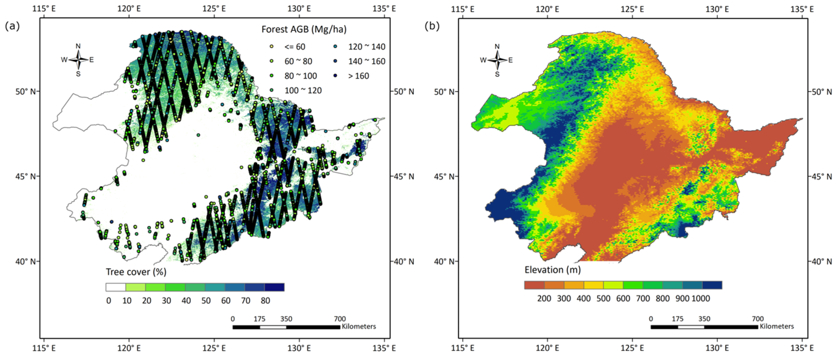
2.1. Study Area
2.2. Forest AGB Data
2.3. Landsat Data
2.4. PALSAR Data
2.5. Topographical Data

| Variables | Descriptions | References |
|---|---|---|
| Green, Red, NIR, SWIR2 | Four spectral metrics extracted from Landsat TM 5 band 2, band 3, band 4, and band 6. | |
| NDVI | (TM4 − TM3)/(TM4 + TM3) | [74] |
| EVI | 2.5 × (TM4 − TM3)/(TM4 + 6 × TM3 − 7.5 × TM1 + 1) | [75] |
| SAVI | 1.5 × (TM4 − TM3)/(TM4 + TM3 + 0.5) | [76] |
| NDMI | (TM4 – TM5)/(TM4 + TM5) | [77,78] |
| SI | TM4/TM5 | [79] |
| NBR | (TM4 – TM7)/(TM4 + TM7) | [80] |
| TCB | B × [TM1, TM2, TM3, TM4, TM5, TM7, 1]T | [81] |
| TCG | G × [TM1, TM2, TM3, TM4, TM5, TM7, 1]T | [81] |
| TCW | W × [TM1, TM2, TM3, TM4, TM5, TM7, 1]T | [81] |
| TCD | [82] | |
| TCA | artan(TCG/TCB) | [83] |
| TM texture | Four GLCM texture measures (mean, variance, correlation, homogeneity) extracted from each spectral band. | [84] |
| FVC | The metrics were extracted from the global tree cover data published by Hansen. | [68] |
| HH, HV | PALSAR backscatter coefficients. | |
| HH−HV, HH/HV | The difference and ratio values between HH and HV. | [71] |
| PALSAR texture | GLCM texture measure associated with HH and HV. | |
| Elevation, Slope | Topographical predictors. |
2.6. FS Methods
2.6.1. Boruta
2.6.2. JMIM
2.6.3. RFE
2.6.4. MDA
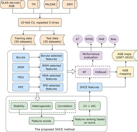
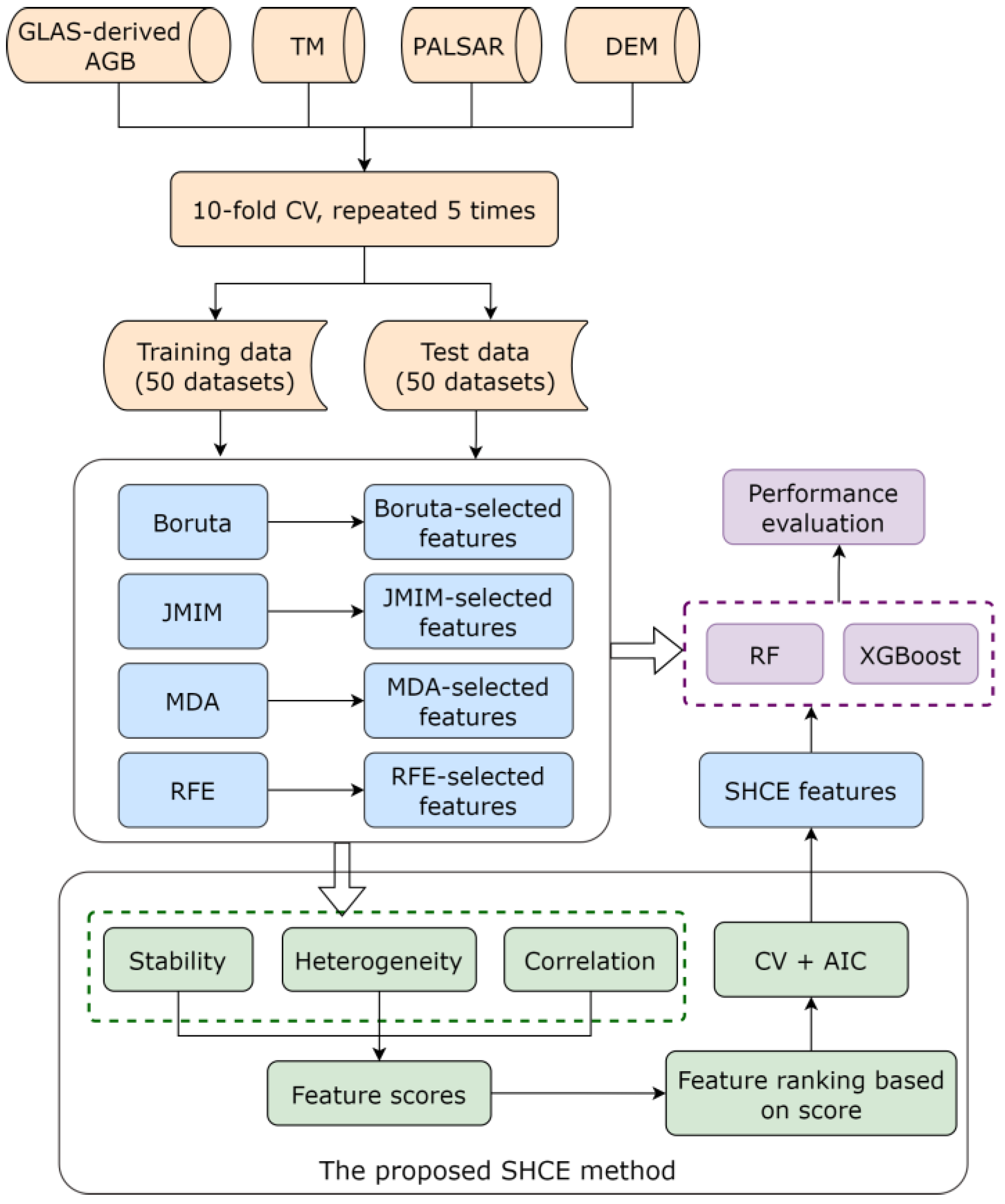
2.6.5. Proposed Ensemble FS Algorithm
2.7. AGB Modelling
2.8. Evaluation Metrics
3. Results
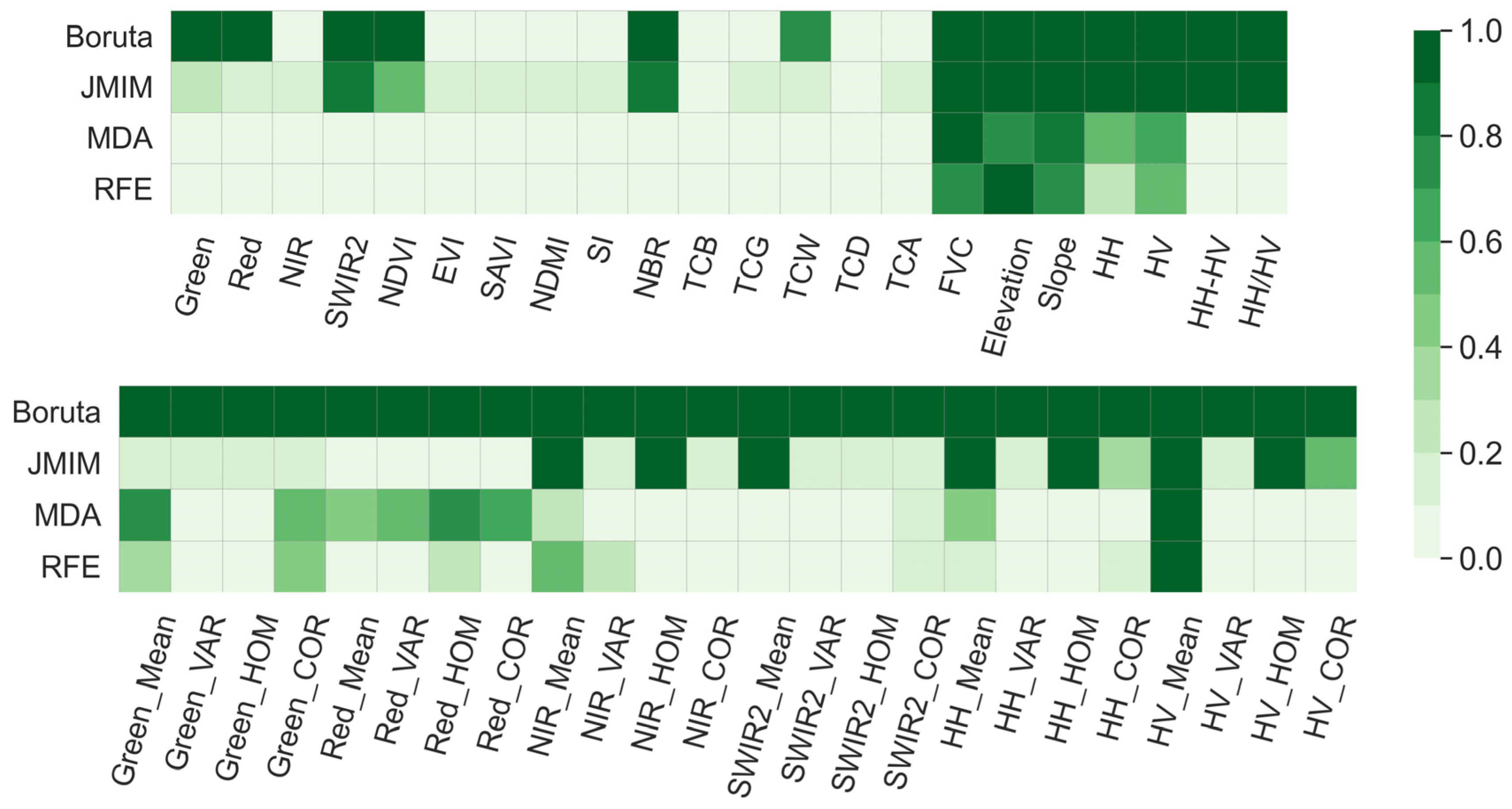
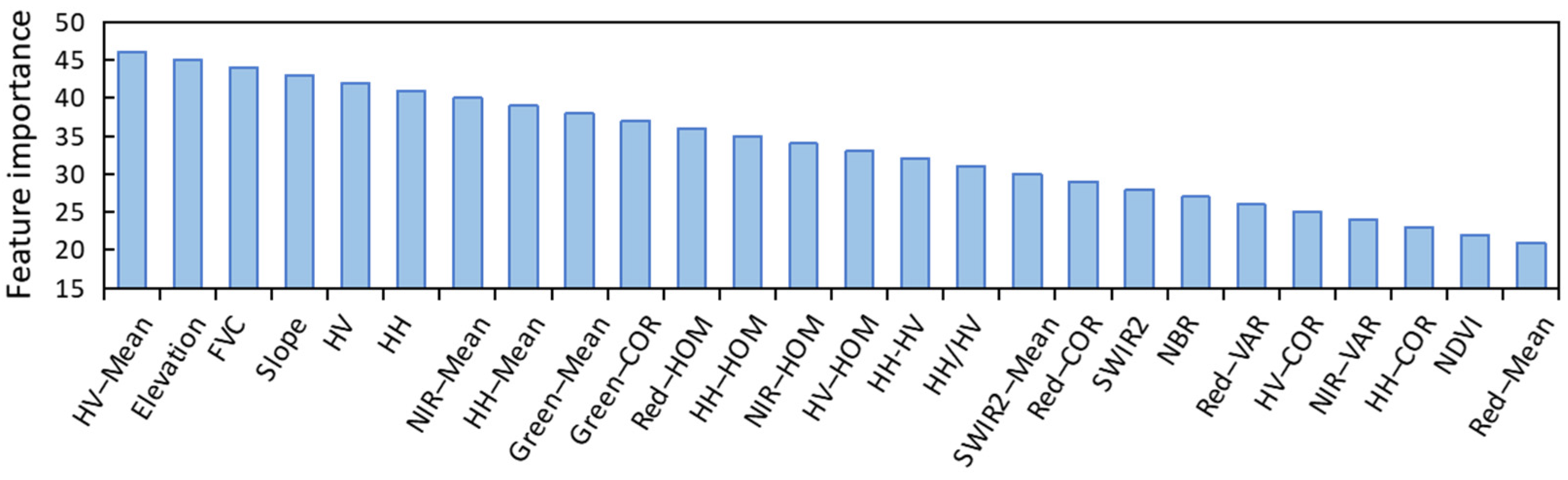
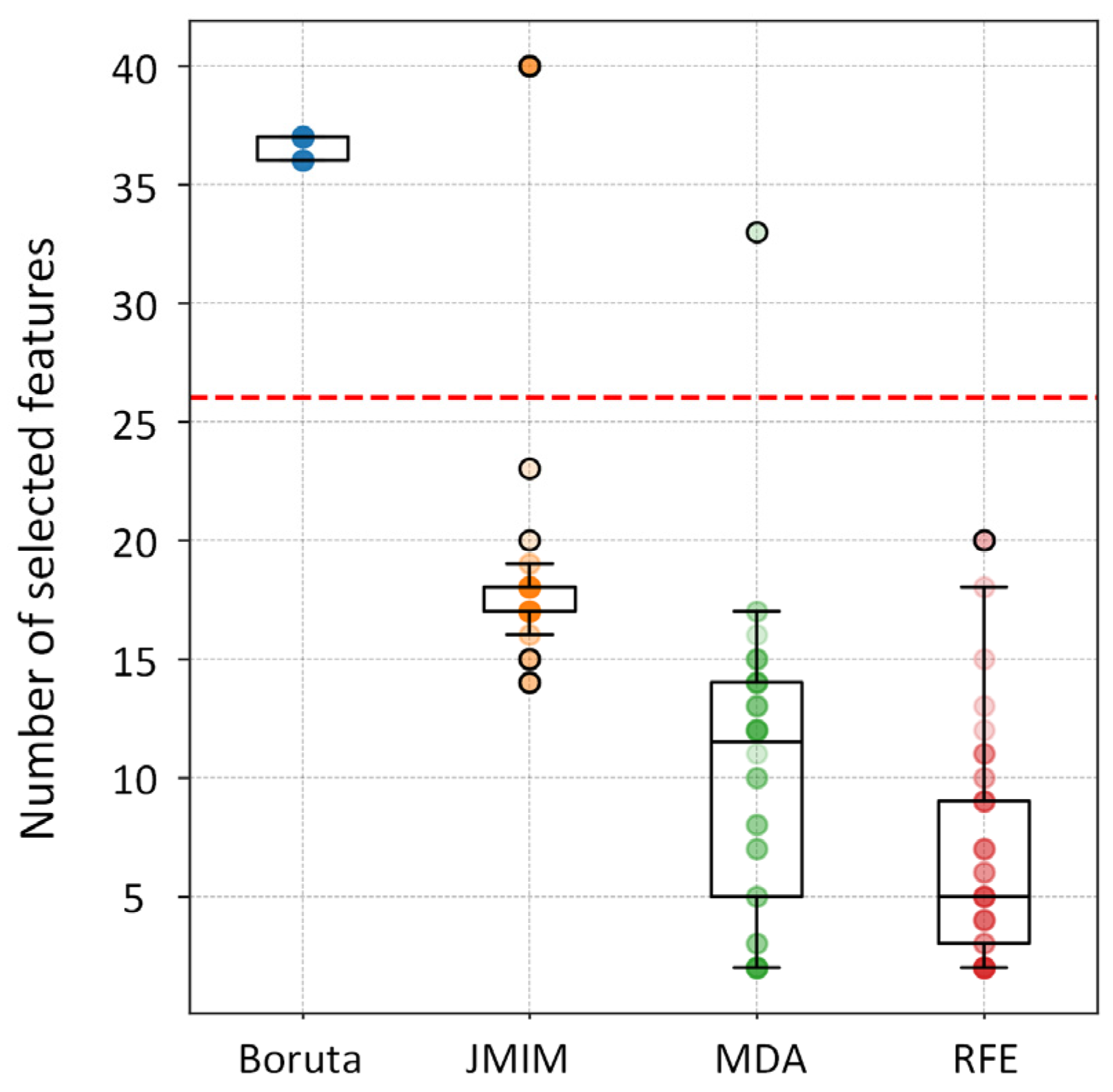
3.1. Important Features Identified for Forest AGB Prediction
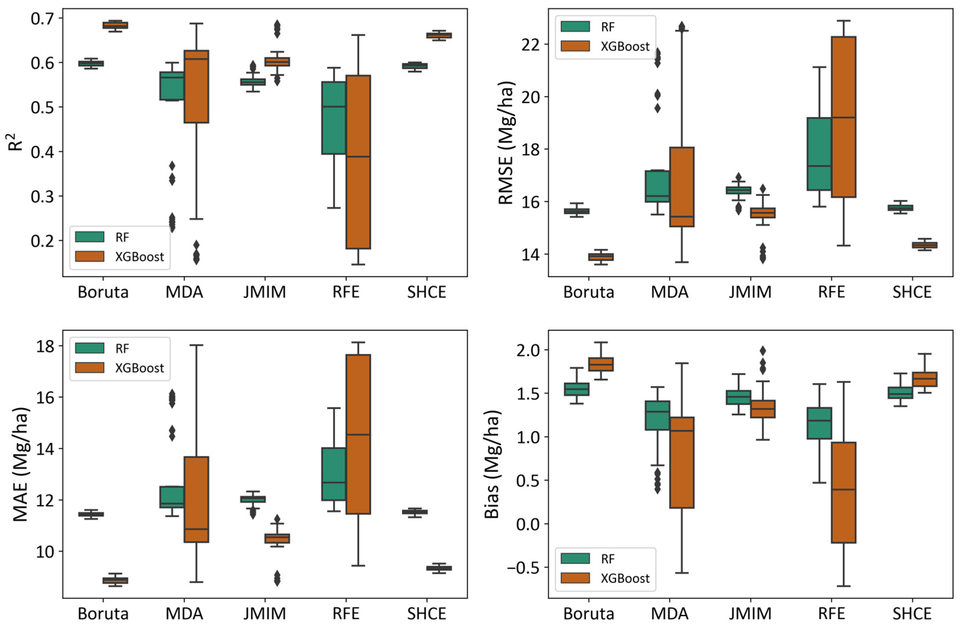
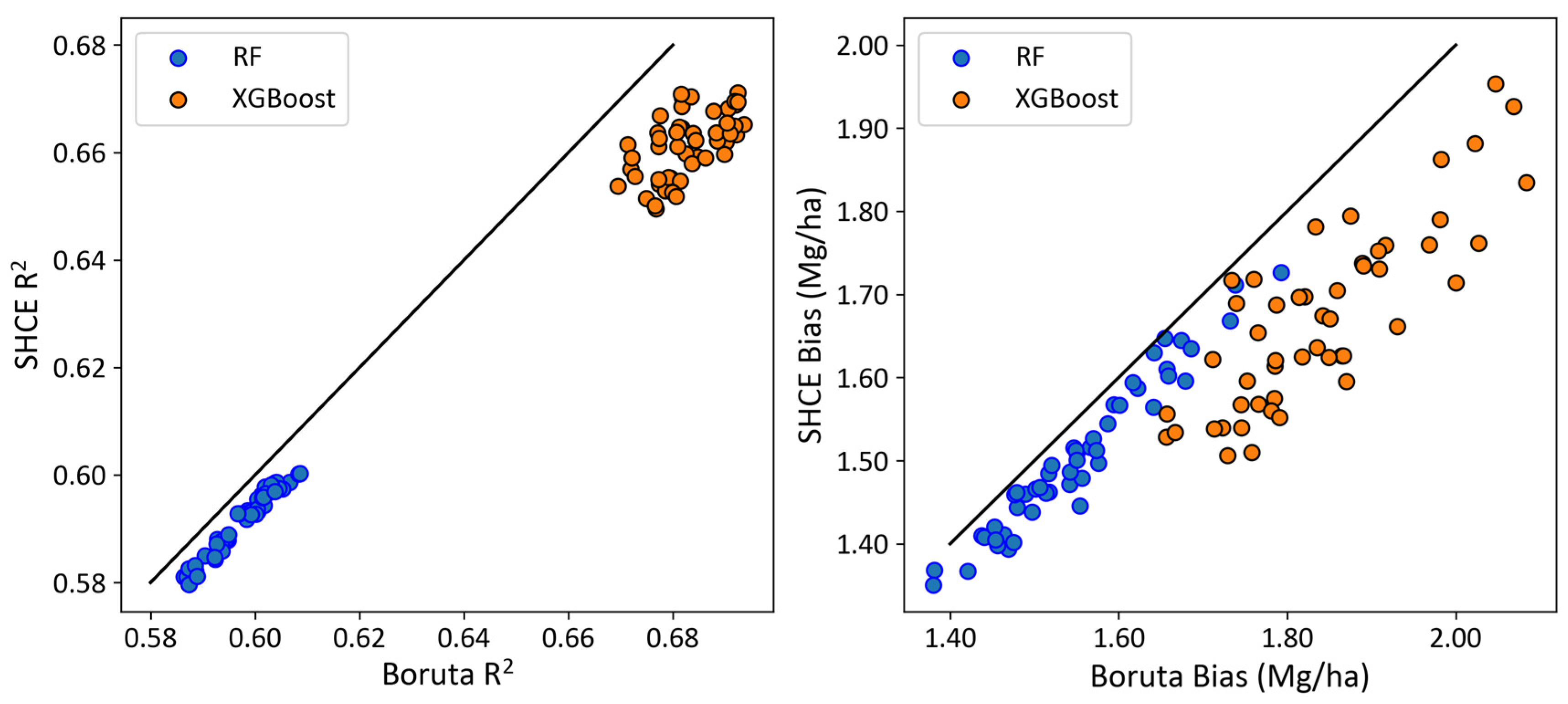
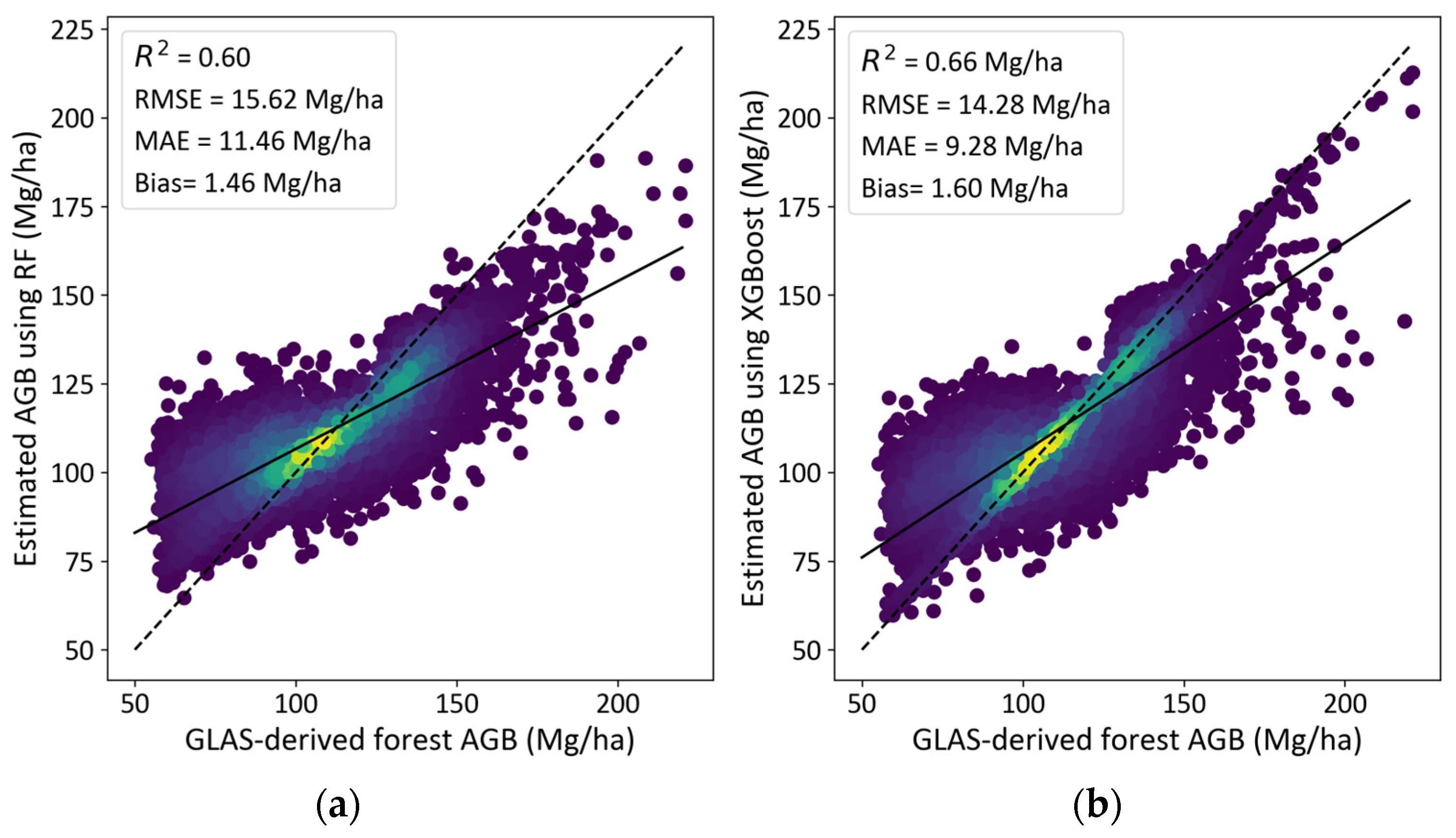
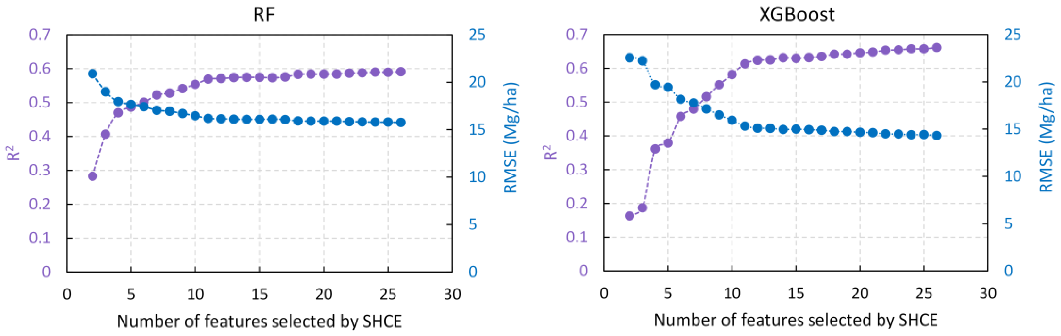
3.2. Accuracy of Forest AGB Prediction Based on Selected Features
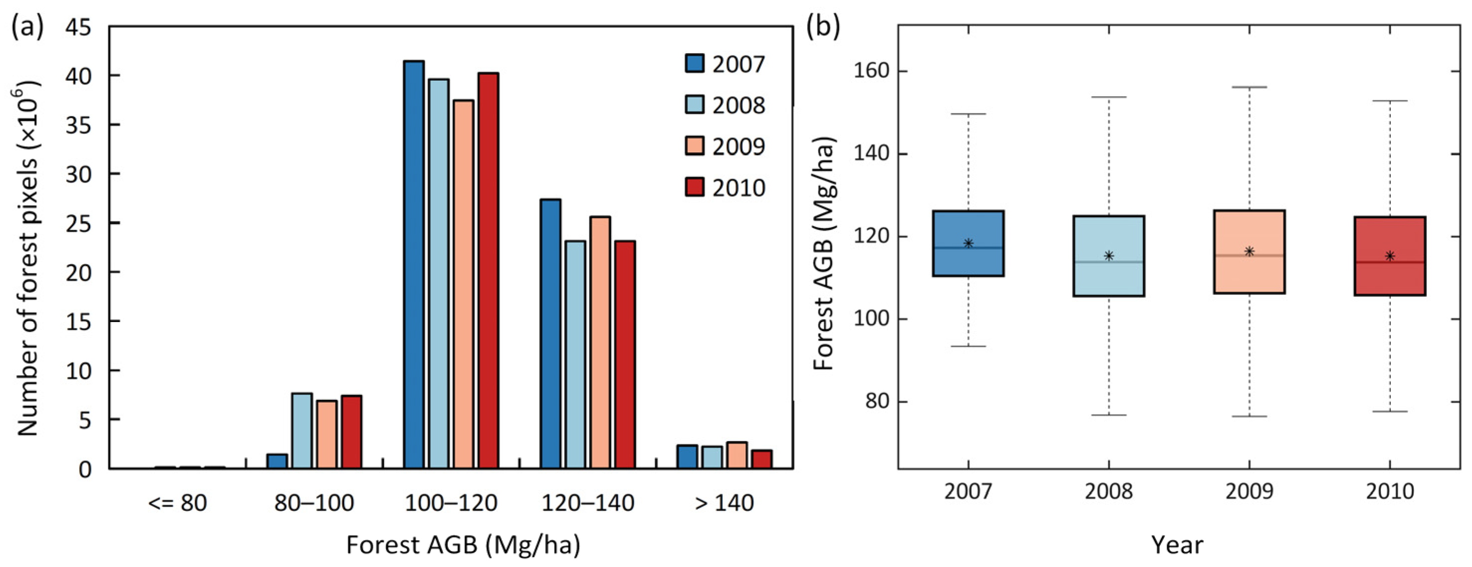
3.3. Forest AGB Maps at 90 m Resolution
4. Discussion
4.1. The Significance of SHCE in Predicting Forest AGB
4.2. Identified Important Features for Forest AGB Prediction
4.3. Comparison of Forest AGB Maps with Other Studies
4.4. Limitations of This Study
5. Conclusions
Author Contributions
Funding
Conflicts of Interest
References
- Le Toan, T.; Quegan, S.; Davidson, M.W.J.; Balzter, H.; Paillou, P.; Papathanassiou, K.; Plummer, S.; Rocca, F.; Saatchi, S.; Shugart, H.; et al. The BIOMASS mission: Mapping global forest biomass to better understand the terrestrial carbon cycle. Remote Sens. Environ. 2011, 115, 2850–2860. [Google Scholar] [CrossRef] [Green Version]
- Pan, Y.; Birdsey, R.A.; Phillips, O.L.; Jackson, R.B. The Structure, Distribution, and Biomass of the World’s Forests. Annu. Rev. Ecol. Evol. Syst. 2013, 44, 593–622. [Google Scholar] [CrossRef] [Green Version]
- Mitchard, E.T.A. The tropical forest carbon cycle and climate change. Nature 2018, 559, 527–534. [Google Scholar] [CrossRef] [PubMed] [Green Version]
- Saatchi, S.S.; Harris, N.L.; Brown, S.; Lefsky, M.; Mitchard, E.T.A.; Salas, W.; Zutta, B.R.; Buermann, W.; Lewis, S.L.; Hagen, S.; et al. Benchmark map of forest carbon stocks in tropical regions across three continents. Proc. Natl. Acad. Sci. USA 2011, 108, 9899–9904. [Google Scholar] [CrossRef] [PubMed] [Green Version]
- Quegan, S.; Toan, T.L.; Chave, J.; Dall, J.; Williams, M. The European Space Agency BIOMASS mission: Measuring forest above-ground biomass from space. Remote Sens. Environ. 2019, 227, 44–60. [Google Scholar] [CrossRef] [Green Version]
- Heiskanen, J. Estimating aboveground tree biomass and leaf area index in a mountain birch forest using ASTER satellite data. Int. J. Remote Sens. 2006, 27, 1135–1158. [Google Scholar] [CrossRef]
- Sun, Z.; Peng, S.; Li, X.; Guo, Z.; Piao, S. Changes in forest biomass over China during the 2000s and implications for management. For. Ecol. Manag. 2015, 357, 76–83. [Google Scholar] [CrossRef]
- Motlagh, M.G.; Kafaky, S.B.; Mataji, A.; Akhavan, R. Estimating and mapping forest biomass using regression models and Spot-6 images (case study: Hyrcanian forests of north of Iran). Environ. Monit. Assess. 2018, 190, 352. [Google Scholar] [CrossRef]
- Poulain, M.; Pena, M.; Schmidt, A.; Schmidt, H.; Schulte, A. Relationships between forest variables and remote sensing data in a Nothofagus pumilio forest. Geocarto Int. 2010, 25, 25–43. [Google Scholar] [CrossRef]
- Meng, S.; Pang, Y.; Zhang, Z.; Jia, W.; Li, Z. Mapping Aboveground Biomass using Texture Indices from Aerial Photos in a Temperate Forest of Northeastern China. Remote Sens. 2016, 8, 230. [Google Scholar] [CrossRef] [Green Version]
- Zhuang, W.; Mountrakis, G.; Wiley, J.J.; Beier, C.M. Estimation of above-ground forest biomass using metrics based on Gaussian decomposition of waveform lidar data. Int. J. Remote Sens. 2015, 36, 1871–1889. [Google Scholar] [CrossRef]
- Popescu, S.C.; Zhao, K.; Neuenschwander, A.; Lin, C. Satellite lidar vs. small footprint airborne lidar: Comparing the accuracy of aboveground biomass estimates and forest structure metrics at footprint level. Remote Sens. Environ. 2011, 115, 2786–2797. [Google Scholar] [CrossRef]
- Debastiani, A.B.; Sanquetta, C.R.; Dalla Corte, A.P.; Rex, F.E.; Pinto, N.S. Evaluating SAR-optical sensor fusion for aboveground biomass estimation in a Brazilian tropical forest. Ann. For. Res. 2019, 62, 109–122. [Google Scholar] [CrossRef]
- Yu, H.; Zhang, Z. The Performance of Relative Height Metrics for Estimation of Forest Above-Ground Biomass Using L- and X-Bands TomoSAR Data. IEEE J. Sel. Top. Appl. Earth Obs. Remote Sens. 2021, 14, 1857–1871. [Google Scholar] [CrossRef]
- Zhang, Y.; Ma, J.; Liang, S.; Li, X.; Li, M. An Evaluation of Eight Machine Learning Regression Algorithms for Forest Aboveground Biomass Estimation from Multiple Satellite Data Products. Remote Sens. 2020, 12, 4015. [Google Scholar] [CrossRef]
- Gleason, C.J.; Im, J. Forest biomass estimation from airborne LiDAR data using machine learning approaches. Remote Sens. Environ. 2012, 125, 80–91. [Google Scholar] [CrossRef]
- Ghosh, S.M.; Behera, M.D. Aboveground biomass estimation using multi-sensor data synergy and machine learning algorithms in a dense tropical forest. Appl. Geogr. 2018, 96, 29–40. [Google Scholar] [CrossRef]
- Shao, Z.; Zhang, L.; Wang, L. Stacked Sparse Autoencoder Modeling Using the Synergy of Airborne LiDAR and Satellite Optical and SAR Data to Map Forest Above-Ground Biomass. IEEE J. Sel. Top. Appl. Earth Obs. Remote Sens. 2017, 10, 5569–5582. [Google Scholar] [CrossRef]
- Saeys, Y.; Inza, I.; Larrañaga, P. A review of feature selection techniques in bioinformatics. Bioinformatics 2007, 23, 2507–2517. [Google Scholar] [CrossRef] [Green Version]
- Wang, L.; Wang, Y.; Chang, Q. Feature selection methods for big data bioinformatics: A survey from the search perspective. Methods 2016, 111, 21–31. [Google Scholar] [CrossRef]
- Bolón-Canedo, V.; Remeseiro, B. Feature selection in image analysis: A survey. Artif. Intell. Rev. 2020, 53, 2905–2931. [Google Scholar] [CrossRef]
- Huang, L.; Ran, J.; Wang, W.; Yang, T.; Xiang, Y. A multi-channel anomaly detection method with feature selection and multi-scale analysis. Comput. Netw. 2021, 185, 107645. [Google Scholar] [CrossRef]
- Teh, H.Y.; Wang, K.I.K.; Kempa-Liehr, A.W. Expect the Unexpected: Unsupervised Feature Selection for Automated Sensor Anomaly Detection. IEEE Sens. J. 2021, 21, 18033–18046. [Google Scholar] [CrossRef]
- Abualigah, L.M.; Khader, A.T. Unsupervised text feature selection technique based on hybrid particle swarm optimization algorithm with genetic operators for the text clustering. J. Supercomput. 2017, 73, 4773–4795. [Google Scholar] [CrossRef]
- Guyon, I.; Elisseeff, A. An introduction to variable and feature selection. J. Mach. Learn. Res. 2003, 3, 1157–1182. [Google Scholar]
- Hsu, H.-H.; Hsieh, C.-W.; Lu, M.-D. Hybrid feature selection by combining filters and wrappers. Expert Syst. Appl. 2011, 38, 8144–8150. [Google Scholar] [CrossRef]
- Huang, N.; Li, R.; Lin, L.; Yu, Z.; Cai, G. Low Redundancy Feature Selection of Short Term Solar Irradiance Prediction Using Conditional Mutual Information and Gauss Process Regression. Sustainability 2018, 10, 2889. [Google Scholar] [CrossRef] [Green Version]
- Zolkos, S.G.; Goetz, S.J.; Dubayah, R. A meta-analysis of terrestrial aboveground biomass estimation using lidar remote sensing. Remote Sens. Environ. 2013, 128, 289–298. [Google Scholar] [CrossRef]
- Fassnacht, F.E.; Hartig, F.; Latifi, H.; Berger, C.; Hernandez, J.; Corvalan, P.; Koch, B. Importance of sample size, data type and prediction method for remote sensing-based estimations of aboveground forest biomass. Remote Sens. Environ. 2014, 154, 102–114. [Google Scholar] [CrossRef]
- Cai, J.; Luo, J.W.; Wang, S.L.; Yang, S. Feature selection in machine learning: A new perspective. Neurocomputing 2018, 300, 70–79. [Google Scholar] [CrossRef]
- Archibald, R.; Fann, G. Feature selection and classification of hyperspectral images, with support vector machines. IEEE Geosci. Remote Sens. Lett. 2007, 4, 674–677. [Google Scholar] [CrossRef]
- Chandrashekar, G.; Sahin, F. A survey on feature selection methods. Comput. Electr. Eng. 2014, 40, 16–28. [Google Scholar] [CrossRef]
- Liu, H.; Zhou, M.; Liu, Q. An embedded feature selection method for imbalanced data classification. IEEE/CAA J. Autom. Sin. 2019, 6, 703–715. [Google Scholar] [CrossRef]
- Xie, Z.; Xu, Y. Sparse group LASSO based uncertain feature selection. Int. J. Mach. Learn. Cybern. 2014, 5, 201–210. [Google Scholar] [CrossRef]
- Hancer, E.; Xue, B.; Zhang, M.J. Differential evolution for filter feature selection based on information theory and feature ranking. Knowl.-Based Syst. 2018, 140, 103–119. [Google Scholar] [CrossRef]
- Moradi, P.; Gholampour, M. A hybrid particle swarm optimization for feature subset selection by integrating a novel local search strategy. Appl. Soft Comput. 2016, 43, 117–130. [Google Scholar] [CrossRef]
- Zorarpacı, E.; Özel, S.A. A hybrid approach of differential evolution and artificial bee colony for feature selection. Expert Syst. Appl. 2016, 62, 91–103. [Google Scholar] [CrossRef]
- Got, A.; Moussaoui, A.; Zouache, D. Hybrid filter-wrapper feature selection using whale optimization algorithm: A multi-objective approach. Expert Syst. Appl. 2021, 183, 115312. [Google Scholar] [CrossRef]
- Chuang, L.-Y.; Yang, C.-H.; Wu, K.-C.; Yang, C.-H. A hybrid feature selection method for DNA microarray data. Comput. Biol. Med. 2011, 41, 228–237. [Google Scholar] [CrossRef] [PubMed]
- Pes, B.; Dessì, N.; Angioni, M. Exploiting the ensemble paradigm for stable feature selection: A case study on high-dimensional genomic data. Inf. Fusion 2017, 35, 132–147. [Google Scholar] [CrossRef]
- Wang, X.P.; Fang, J.Y.; Zhu, B. Forest biomass and root-shoot allocation in northeast China. For. Ecol. Manag. 2008, 255, 4007–4020. [Google Scholar] [CrossRef]
- Yao, Y.; Wang, X.; Li, Y.; Wang, T.; Shen, M.; Du, M.; He, H.; Li, Y.; Luo, W.; Ma, M.; et al. Spatiotemporal pattern of gross primary productivity and its covariation with climate in China over the last thirty years. Glob. Chang. Biol. 2017, 24, 184–196. [Google Scholar] [CrossRef] [PubMed]
- Pan, Y.; Birdsey, R.A.; Fang, J.; Houghton, R.; Kauppi, P.E.; Kurz, W.A.; Phillips, O.L.; Shvidenko, A.; Lewis, S.L.; Canadell, J.G.; et al. A Large and Persistent Carbon Sink in the World’s Forests. Science 2011, 333, 988–993. [Google Scholar] [CrossRef] [PubMed] [Green Version]
- Zhou, Y.L. Geography of the Vegetation in Northeast China; Science Press: Beijing, China, 1997. [Google Scholar]
- Zhang, Y.; Liang, S.; Sun, G. Forest biomass mapping of Northeastern China Using GLAS and MODIS Data. IEEE J. Sel. Top. Appl. Earth Obs. Remote Sens. 2014, 7, 140–152. [Google Scholar] [CrossRef]
- Sun, G.; Ranson, K.J.; Masek, J.; Guo, Z.; Pang, Y.; Fu, A.; Wang, D. Estimation of Tree Height and Forest Biomass from GLAS Data. J. For. Plan. 2008, 13, 157–164. [Google Scholar]
- Pang, Y.; Lefsky, M.; Sun, G.; Miller, M.E.; Li, Z. Temperate forest height estimation performance using ICESat GLAS data from different observation periods. Int. Arch. Photogramm. Remote Sens. Spat. Inf. Sci. 2008, 37, 777–782. [Google Scholar]
- Chi, H.; Sun, G.; Huang, J.; Guo, Z.; Ni, W.; Fu, A. National Forest Aboveground Biomass Mapping from ICESat/GLAS Data and MODIS Imagery in China. Remote Sens. 2015, 7, 5534–5564. [Google Scholar] [CrossRef] [Green Version]
- Zhang, Y.; Li, W.; Liang, S. New Metrics and the Combinations for Estimating Forest Biomass from GLAS Data. IEEE J. Sel. Top. Appl. Earth Obs. Remote Sens. 2021, 14, 7830–7839. [Google Scholar] [CrossRef]
- Lee, S.; Ni-Meister, W.; Yang, W.; Qi, C. Physically based vertical vegetation structure retrieval from ICESat data: Validation using LVIS in White Mountain National Forest, New Hampshire, USA. Remote Sens. Environ. 2011, 115, 2776–2785. [Google Scholar] [CrossRef]
- Simard, M.; Pinto, N.; Fisher, J.B.; Baccini, A. Mapping forest canopy height globally with spaceborne lidar. J. Geophys. Res. Biogeosci. 2011, 116, G04021. [Google Scholar] [CrossRef] [Green Version]
- Branco, P.; Torgo, L.; Ribeiro, R.P. SMOGN: A Pre-processing Approach for Imbalanced Regression. In Proceedings of the First International Workshop on Learning with Imbalanced Domains: Theory and Applications, Skopje, Macedonia, 22 September 2017; Paula Branco Luís, T., Nuno, M., Eds.; PMLR: London, UK, 2017; pp. 36–50. [Google Scholar]
- Dwyer, J.L.; Roy, D.P.; Sauer, B.; Jenkerson, C.B.; Lymburner, L. Analysis Ready Data: Enabling Analysis of the Landsat Archive. Remote Sens. 2018, 10, 1363. [Google Scholar] [CrossRef]
- Wulder, M.A.; Loveland, T.R.; Roy, D.P.; Crawford, C.J.; Masek, J.G.; Woodcock, C.E.; Allen, R.G.; Anderson, M.C.; Belward, A.S.; Cohen, W.B.; et al. Current status of Landsat program, science, and applications. Remote Sens. Environ. 2019, 225, 127–147. [Google Scholar] [CrossRef]
- Amani, M.; Ghorbanian, A.; Ahmadi, S.A.; Kakooei, M.; Moghimi, A.; Mirmazloumi, S.M.; Moghaddam, S.H.A.; Mahdavi, S.; Ghahremanloo, M.; Parsian, S.; et al. Google Earth Engine Cloud Computing Platform for Remote Sensing Big Data Applications: A Comprehensive Review. IEEE J. Sel. Top. Appl. Earth Obs. Remote Sens. 2020, 13, 5326–5350. [Google Scholar] [CrossRef]
- Gorelick, N.; Hancher, M.; Dixon, M.; Ilyushchenko, S.; Thau, D.; Moore, R. Google Earth Engine: Planetary-scale geospatial analysis for everyone. Remote Sens. Environ. 2017, 202, 18–27. [Google Scholar] [CrossRef]
- Luo, M.; Wang, Y.; Xie, Y.; Zhou, L.; Qiao, J.; Qiu, S.; Sun, Y. Combination of feature selection and catboost for prediction: The first application to the estimation of aboveground biomass. Forests 2021, 12, 216. [Google Scholar] [CrossRef]
- Lu, D.; Chen, Q.; Wang, G.; Liu, L.; Li, G.; Moran, E. A survey of remote sensing-based aboveground biomass estimation methods in forest ecosystems. Int. J. Digit. Earth 2016, 9, 63–105. [Google Scholar] [CrossRef]
- Wu, C.; Shen, H.; Shen, A.; Deng, J.; Gan, M.; Zhu, J.; Xu, H.; Wang, K. Comparison of machine-learning methods for above-ground biomass estimation based on Landsat imagery. J. Appl. Remote Sens. 2016, 10, 035010. [Google Scholar] [CrossRef]
- Frazier, R.J.; Coops, N.C.; Wulder, M.A.; Kennedy, R. Characterization of aboveground biomass in an unmanaged boreal forest using Landsat temporal segmentation metrics. ISPRS J. Photogramm. Remote Sens. 2014, 92, 137–146. [Google Scholar] [CrossRef]
- Gomez, C.; White, J.C.; Wulder, M.A.; Alejandro, P. Historical forest biomass dynamics modelled with Landsat spectral trajectories. ISPRS J. Photogramm. Remote Sens. 2014, 93, 14–28. [Google Scholar] [CrossRef] [Green Version]
- Zald, H.S.J.; Wulder, M.A.; White, J.C.; Hilker, T.; Hermosilla, T.; Hobart, G.W.; Coops, N.C. Integrating Landsat pixel composites and change metrics with lidar plots to predictively map forest structure and aboveground biomass in Saskatchewan, Canada. Remote Sens. Environ. 2016, 176, 188–201. [Google Scholar] [CrossRef] [Green Version]
- Lu, D.; Batistella, M. Exploring TM image texture and its relationships with biomass estimation in Rondônia, Brazilian Amazon. Acta Amaz. 2005, 35, 249–257. [Google Scholar] [CrossRef]
- Liao, Z.; He, B.; Quan, X. Potential of texture from SAR tomographic images for forest aboveground biomass estimation. Int. J. Appl. Earth Obs. Geoinf. 2020, 88, 102049. [Google Scholar] [CrossRef]
- Eckert, S. Improved Forest Biomass and Carbon Estimations Using Texture Measures from WorldView-2 Satellite Data. Remote Sens. 2012, 4, 810–829. [Google Scholar] [CrossRef] [Green Version]
- Kelsey, K.C.; Neff, J.C. Estimates of Aboveground Biomass from Texture Analysis of Landsat Imagery. Remote Sens. 2014, 6, 6407–6422. [Google Scholar] [CrossRef] [Green Version]
- Clausi, D.A. An analysis of co-occurrence texture statistics as a function of grey level quantization. Can. J. Remote Sens. 2002, 28, 45–62. [Google Scholar] [CrossRef]
- Hansen, M.C.; Potapov, P.V.; Moore, R.; Hancher, M.; Turubanova, S.A.; Tyukavina, A.; Thau, D.; Stehman, S.V.; Goetz, S.J.; Loveland, T.R.; et al. High-Resolution Global Maps of 21st-Century Forest Cover Change. Science 2013, 342, 850–853. [Google Scholar] [CrossRef] [PubMed] [Green Version]
- Shimada, M.; Ohtaki, T. Generating Large-Scale High-Quality SAR Mosaic Datasets: Application to PALSAR Data for Global Monitoring. IEEE J. Sel. Top. Appl. Earth Obs. Remote Sens. 2010, 3, 637–656. [Google Scholar] [CrossRef]
- Shimada, M.; Itoh, T.; Motooka, T.; Watanabe, M.; Shiraishi, T.; Thapa, R.; Lucas, R. New global forest/non-forest maps from ALOS PALSAR data (2007–2010). Remote Sens. Environ. 2014, 155, 13–31. [Google Scholar] [CrossRef]
- Shen, W.; Li, M.; Huang, C.; Tao, X.; Wei, A. Annual forest aboveground biomass changes mapped using ICESat/GLAS measurements, historical inventory data, and time-series optical and radar imagery for Guangdong province, China. Agric. For. Meteorol. 2018, 259, 23–38. [Google Scholar] [CrossRef] [Green Version]
- Zhang, Y.; Ling, F.; Foody, G.M.; Ge, Y.; Boyd, D.S.; Li, X.; Du, Y.; Atkinson, P.M. Mapping annual forest cover by fusing PALSAR/PALSAR-2 and MODIS NDVI during 2007–2016. Remote Sens. Environ. 2019, 224, 74–91. [Google Scholar] [CrossRef] [Green Version]
- Jarvis, A.; Reuter, H.I.; Nelson, A.; Guevara, E. Hole-filled SRTM for the globe Version 4. 2008. Available online: http://srtm.csi.cgiar.org (accessed on 31 December 2021).
- Rouse, J.W.; Haas, R.H.; Schell, J.A.; Deering, D.W. Monitoring Vegetation Systems in the Great Plains with ERTS. NASA Spec. Publ. 1974, 351, 309. [Google Scholar]
- Huete, A.; Didan, K.; Miura, T.; Rodriguez, E.P.; Gao, X.; Ferreira, L.G. Overview of the radiometric and biophysical performance of the MODIS vegetation indices. Remote Sens. Environ. 2002, 83, 195–213. [Google Scholar] [CrossRef]
- Huete, A.R. A soil-adjusted vegetation index (SAVI). Remote Sens. Environ. 1988, 25, 295–309. [Google Scholar] [CrossRef]
- Wilson, E.H.; Sader, S.A. Detection of forest harvest type using multiple dates of Landsat TM imagery. Remote Sens. Environ. 2002, 80, 385–396. [Google Scholar] [CrossRef]
- Hardisky, M.A.; Klemas, V.; Smart, R.M. The influence of soil salinity, growth form, and leaf moisture on the spectral radiance of Spartina Alterniflora canopies. Photogramm. Eng. Remote Sens. 1983, 48, 77–84. [Google Scholar]
- Fiorella, M.; Ripple, W.J. Determining successional stage of temperate coniferous forests with Landsat satellite data. Photogramm. Eng. Remote Sens. 1993, 59, 239–246. [Google Scholar]
- López García, M.J.; Caselles, V. Mapping burns and natural reforestation using thematic Mapper data. Geocarto Int. 1991, 6, 31–37. [Google Scholar] [CrossRef]
- Crist, E.P. A TM Tasseled Cap equivalent transformation for reflectance factor data. Remote Sens. Environ. 1985, 17, 301–306. [Google Scholar] [CrossRef]
- Duane, M.V.; Cohen, W.B.; Campbell, J.L.; Hudiburg, T.; Turner, D.P.; Weyermann, D.L. Implications of Alternative Field-Sampling Designs on Landsat-Based Mapping of Stand Age and Carbon Stocks in Oregon Forests. For. Sci. 2010, 56, 405–416. [Google Scholar]
- Powell, S.L.; Cohen, W.B.; Healey, S.P.; Kennedy, R.E.; Moisen, G.G.; Pierce, K.B.; Ohmann, J.L. Quantification of live aboveground forest biomass dynamics with Landsat time-series and field inventory data: A comparison of empirical modeling approaches. Remote Sens. Environ. 2010, 114, 1053–1068. [Google Scholar] [CrossRef]
- Haralick, R.M.; Shanmugam, K.; Dinstein, I. Textural Features for Image Classification. IEEE Trans. Syst. Man Cybern. 1973, SMC-3, 610–621. [Google Scholar] [CrossRef] [Green Version]
- Kursa, M.B.; Rudnicki, W.R. Feature Selection with the Boruta Package. J. Stat. Softw. 2010, 36, 13. [Google Scholar] [CrossRef] [Green Version]
- Degenhardt, F.; Seifert, S.; Szymczak, S. Evaluation of variable selection methods for random forests and omics data sets. Brief. Bioinform. 2017, 20, 492–503. [Google Scholar] [CrossRef] [PubMed] [Green Version]
- Battiti, R. Using mutual information for selecting features in supervised neural net learning. IEEE Trans. Neural Netw. 1994, 5, 537–550. [Google Scholar] [CrossRef] [PubMed] [Green Version]
- Peng, H.; Long, F.; Ding, C. Feature selection based on mutual information criteria of max-dependency, max-relevance, and min-redundancy. IEEE Trans. Pattern Anal. Mach. Intell. 2005, 27, 1226–1238. [Google Scholar] [CrossRef] [PubMed]
- Bennasar, M.; Hicks, Y.; Setchi, R. Feature selection using Joint Mutual Information Maximisation. Expert Syst. Appl. 2015, 42, 8520–8532. [Google Scholar] [CrossRef] [Green Version]
- Ross, B.C. Mutual Information between Discrete and Continuous Data Sets. PLoS ONE 2014, 9, e87357. [Google Scholar] [CrossRef]
- Guyon, I.; Weston, J.; Barnhill, S.; Vapnik, V. Gene Selection for Cancer Classification using Support Vector Machines. Mach. Learn. 2002, 46, 389–422. [Google Scholar] [CrossRef]
- Rasel, S.M.M.; Chang, H.C.; Ralph, T.J.; Saintilan, N.; Diti, I.J. Application of feature selection methods and machine learning algorithms for saltmarsh biomass estimation using Worldview-2 imagery. Geocarto Int. 2021, 36, 1075–1099. [Google Scholar] [CrossRef]
- Georganos, S.; Grippa, T.; Vanhuysse, S.; Lennert, M.; Shimoni, M.; Kalogirou, S.; Wolff, E. Less is more: Optimizing classification performance through feature selection in a very-high-resolution remote sensing object-based urban application. GIScience Remote Sens. 2018, 55, 221–242. [Google Scholar] [CrossRef]
- Chrysafis, I.; Mallinis, G.; Gitas, I.; Tsakiri-Strati, M. Estimating Mediterranean forest parameters using multi seasonal Landsat 8 OLI imagery and an ensemble learning method. Remote Sens. Environ. 2017, 199, 154–166. [Google Scholar] [CrossRef]
- Saeys, Y.; Abeel, T.; Van de Peer, Y. Robust Feature Selection Using Ensemble Feature Selection Techniques. In Proceedings of the Machine Learning and Knowledge Discovery in Databases, European Conference, ECML PKDD 2008, Antwerp, Belgium, 15–19 September 2008; Daelemans, W., Goethals, B., Morik, K., Eds.; Springer: Berlin/Heidelberg, Germany, 2008; pp. 313–325. [Google Scholar]
- Tsai, C.-F.; Sung, Y.-T. Ensemble feature selection in high dimension, low sample size datasets: Parallel and serial combination approaches. Knowl.-Based Syst. 2020, 203, 106097. [Google Scholar] [CrossRef]
- Wang, H.; He, C.; Li, Z. A new ensemble feature selection approach based on genetic algorithm. Soft Comput. 2020, 24, 15811–15820. [Google Scholar] [CrossRef]
- Kuncheva, L.I. A stability index for feature selection. In Proceedings of the IASTED International Conference on Artificial Intelligence and Applications, Innsbruck, Austria, 12–14 February 2007. [Google Scholar]
- Hall, M.A. Correlation-Based Feature Selection for Machine Learning, in Department of Computer Science; University of Waikato: Hamilton, New Zealand, 1999. [Google Scholar]
- Breiman, L. Random Forests. Mach. Learn. 2001, 45, 5–32. [Google Scholar] [CrossRef] [Green Version]
- Belgiu, M.; Drăguţ, L. Random forest in remote sensing: A review of applications and future directions. ISPRS J. Photogramm. Remote Sens. 2016, 114 (Suppl. C), 24–31. [Google Scholar] [CrossRef]
- Zhang, Y.; Liu, J.; Shen, W. A Review of Ensemble Learning Algorithms Used in Remote Sensing Applications. Appl. Sci. 2022, 12, 8654. [Google Scholar] [CrossRef]
- Buhlmann, P.; Hothorn, T. Boosting Algorithms: Regularization, Prediction and Model Fitting. Statist. Sci. 2007, 22, 477–505. [Google Scholar]
- Willmott, C.J.; Matsuura, K. Advantages of the mean absolute error (MAE) over the root mean square error (RMSE) in assessing average model performance. Clim. Res. 2005, 30, 79–82. [Google Scholar] [CrossRef]
- Endres, A.; Endres, A.; Mountrakis, G.; Jin, H.; Zhuang, W.; Manakos, I.; Wiley, J.J.; Beier, C.M. Relative importance analysis of Landsat, waveform LIDAR and PALSAR inputs for deciduous biomass estimation. Eur. J. Remote Sens. 2016, 49, 795–807. [Google Scholar] [CrossRef] [Green Version]
- Sinha, S.; Jeganathan, C.; Sharma, L.K.; Nathawat, M.S.; Das, A.K.; Mohan, S. Developing synergy regression models with space-borne ALOS PALSAR and Landsat TM sensors for retrieving tropical forest biomass. J. Earth Syst. Sci. 2016, 125, 725–735. [Google Scholar] [CrossRef] [Green Version]
- Baghdadi, N.; Le Maire, G.; Bailly, J.S.; Ose, K.; Nouvellon, Y.; Zribi, M.; Lemos, C.; Hakamada, R. Evaluation of ALOS/PALSAR L-Band Data for the Estimation of Eucalyptus Plantations Aboveground Biomass in Brazil. IEEE J. Sel. Top. Appl. Earth Obs. Remote Sens. 2015, 8, 3802–3811. [Google Scholar] [CrossRef] [Green Version]
- Rodríguez-Veiga, P.; Saatchi, S.; Tansey, K.; Balzter, H. Magnitude, spatial distribution and uncertainty of forest biomass stocks in Mexico. Remote Sens. Environ. 2016, 183, 265–281. [Google Scholar] [CrossRef] [Green Version]
- Yang, C.; Huang, H.; Wang, S. Estimation of tropical forest biomass using Landsat TM imagery and permanent plot data in Xishuangbanna, China. Int. J. Remote Sens. 2011, 32, 5741–5756. [Google Scholar] [CrossRef]
- Baccini, A.; Friedl, M.A.; Woodcock, C.E.; Warbington, R. Forest biomass estimation over regional scales using multisource data. Geophys. Res. Lett. 2004, 31, L10501. [Google Scholar] [CrossRef] [Green Version]
- Yang, L.; Liang, S.; Zhang, Y. A New Method for Generating a Global Forest Aboveground Biomass Map from Multiple High-Level Satellite Products and Ancillary Information. IEEE J. Sel. Top. Appl. Earth Obs. Remote Sens. 2020, 13, 2587–2597. [Google Scholar] [CrossRef]
- Zhang, Y.; Liang, S. Fusion of Multiple Gridded Biomass Datasets for Generating a Global Forest Aboveground Biomass Map. Remote Sens. 2020, 12, 2559. [Google Scholar] [CrossRef]
- Tibshirani, R. Regression shrinkage and selection via the lasso: A retrospective. J. R. Stat. Soc. Ser. B (Stat. Methodol.) 2011, 73, 273–282. [Google Scholar] [CrossRef]
- Gheyas, I.A.; Smith, L.S. Feature subset selection in large dimensionality domains. Pattern Recognit. 2010, 43, 5–13. [Google Scholar] [CrossRef] [Green Version]
- Li, B.; Xu, X.; Zhang, L.; Han, J.; Bian, C.; Li, G.; Liu, J.; Jin, L. Above-ground biomass estimation and yield prediction in potato by using UAV-based RGB and hyperspectral imaging. ISPRS J. Photogramm. Remote Sens. 2020, 162, 161–172. [Google Scholar] [CrossRef]
- Robnik-Šikonja, M.; Kononenko, I. Theoretical and Empirical Analysis of ReliefF and RReliefF. Mach. Learn. 2003, 53, 23–69. [Google Scholar] [CrossRef] [Green Version]
- Yu, H.; Wu, Y.; Niu, L.; Chai, Y.; Feng, Q.; Wang, W.; Liang, T. A method to avoid spatial overfitting in estimation of grassland above-ground biomass on the Tibetan Plateau. Ecol. Indic. 2021, 125, 107450. [Google Scholar] [CrossRef]
- Johansen, K.; Morton, M.; Malbeteau, Y.; Aragon, B.; Al-Mashharawi, S.; Ziliani, M.G.; Angel, Y.; Fiene, G.; Negrao, S.; Mousa, M.; et al. Predicting Biomass and Yield in a Tomato Phenotyping Experiment Using UAV Imagery and Random Forest. Front. Artif. Intell. 2020, 3, 28. [Google Scholar] [CrossRef] [PubMed]
- Lu, J.; Wang, H.; Qin, S.; Cao, L.; Pu, R.; Li, G.; Sun, J. Estimation of aboveground biomass of Robinia pseudoacacia forest in the Yellow River Delta based on UAV and Backpack LiDAR point clouds. Int. J. Appl. Earth Obs. Geoinf. 2020, 86, 102014. [Google Scholar] [CrossRef]
- Laurin, G.V.; Chen, Q.; Lindsell, J.A.; Coomes, D.A.; Del Frate, F.; Guerriero, L.; Pirotti, F.; Valenti, R. Above ground biomass estimation in an African tropical forest with lidar and hyperspectral data. ISPRS J. Photogramm. Remote Sens. 2014, 89, 49–58. [Google Scholar] [CrossRef]
- Pandit, S.; Tsuyuki, S.; Dube, T. Landscape-Scale Aboveground Biomass Estimation in Buffer Zone Community Forests of Central Nepal: Coupling In Situ Measurements with Landsat 8 Satellite Data. Remote Sens. 2018, 10, 1848. [Google Scholar] [CrossRef] [Green Version]
- Mutanga, O.; Adam, E.; Cho, M.A. High density biomass estimation for wetland vegetation using WorldView-2 imagery and random forest regression algorithm. Int. J. Appl. Earth Obs. Geoinf. 2012, 18, 399–406. [Google Scholar] [CrossRef]
- Wang, X.; Shao, G.; Chen, H.; Lewis, B.J.; Qi, G.; Yu, D.; Zhou, L.; Dai, L. An Application of Remote Sensing Data in Mapping Landscape-Level Forest Biomass for Monitoring the Effectiveness of Forest Policies in Northeastern China. Environ. Manag. 2013, 52, 612–620. [Google Scholar] [CrossRef]
- Otgonbayar, M.; Atzberger, C.; Chambers, J.; Damdinsuren, A. Mapping pasture biomass in Mongolia using Partial Least Squares, Random Forest regression and Landsat 8 imagery. Int. J. Remote Sens. 2019, 40, 3204–3226. [Google Scholar] [CrossRef]
- Meng, Q.; Meentemeyer, R.K. Modeling of multi-strata forest fire severity using Landsat TM Data. Int. J. Appl. Earth Obs. Geoinf. 2011, 13, 120–126. [Google Scholar] [CrossRef]
- Wulder, M.A.; White, J.C.; Alvarez, F.; Han, T.; Rogan, J.; Hawkes, B. Characterizing boreal forest wildfire with multi-temporal Landsat and LIDAR data. Remote Sens. Environ. 2009, 113, 1540–1555. [Google Scholar] [CrossRef]
- Pflugmacher, D.; Cohen, W.B.; Kennedy, R.E.; Yang, Z. Using Landsat-derived disturbance and recovery history and lidar to map forest biomass dynamics. Remote Sens. Environ. 2014, 151, 124–137. [Google Scholar] [CrossRef]
- Nguyen, T.H.; Jones, S.; Soto-Berelov, M.; Haywood, A.; Hislop, S. Landsat Time-Series for Estimating Forest Aboveground Biomass and Its Dynamics across Space and Time: A Review. Remote Sens. 2020, 12, 98. [Google Scholar] [CrossRef] [Green Version]
- Keeling, H.C.; Phillips, O.L. The global relationship between forest productivity and biomass. Glob. Ecol. Biogeogr. 2007, 16, 618–631. [Google Scholar] [CrossRef]
- Zhang, X.; Kondragunta, S. Estimating forest biomass in the USA using generalized allometric models and MODIS land products. Geophys. Res. Lett. 2006, 33, L09402. [Google Scholar] [CrossRef] [Green Version]
- Liang, S.L.; Cheng, J.; Jia, K.; Jiang, B.; Liu, Q.; Xiao, Z.Q.; Yao, Y.J.; Yuan, W.P.; Zhang, X.T.; Zhao, X.; et al. The Global Land Surface Satellite (GLASS) Product Suite. Bull. Am. Meteorol. Soc. 2021, 102, E323–E337. [Google Scholar] [CrossRef]
- Joetzjer, E.; Pillet, M.; Ciais, P.; Barbier, N.; Chave, J.; Schlund, M.; Maignan, F.; Barichivich, J.; Luyssaert, S.; Herault, B.; et al. Assimilating satellite-based canopy height within an ecosystem model to estimate aboveground forest biomass. Geophys. Res. Lett. 2017, 44, 6823–6832. [Google Scholar] [CrossRef] [Green Version]
- Zhang, Y.; Liang, S.; Yang, L. A review of regional and global gridded forest biomass datasets. Remote Sens. 2019, 11, 2744. [Google Scholar] [CrossRef] [Green Version]
- Tan, K.; Piao, S.; Peng, C.; Fang, J. Satellite-based estimation of biomass carbon stocks for northeast China’s forests between 1982 and 1999. For. Ecol. Manag. 2007, 240, 114–121. [Google Scholar] [CrossRef]
- Zhang, Y.; Liang, S. Changes in forest biomass and linkage to climate and forest disturbances over Northeastern China. Glob. Chang. Biol. 2014, 20, 2596–2606. [Google Scholar] [CrossRef]
- Wang, X.P.; Ouyang, S.; Sun, O.J.; Fang, J.Y. Forest biomass patterns across northeast China are strongly shaped by forest height. For. Ecol. Manag. 2013, 293, 149–160. [Google Scholar] [CrossRef]
- Nandy, S.; Srinet, R.; Padalia, H. Mapping Forest Height and Aboveground Biomass by Integrating ICESat-2, Sentinel-1 and Sentinel-2 Data Using Random Forest Algorithm in Northwest Himalayan Foothills of India. Geophys. Res. Lett. 2021, 48, e2021GL093799. [Google Scholar] [CrossRef]
- Solberg, S.; Nasset, E.; Gobakken, T.; Bollandsas, O.M. Forest biomass change estimated from height change in interferometric SAR height models. Carbon Balance Manag. 2014, 9, 5. [Google Scholar] [CrossRef] [PubMed] [Green Version]
- Chen, L.; Ren, C.Y.; Bao, G.D.; Zhang, B.; Wang, Z.M.; Liu, M.Y.; Man, W.D.; Liu, J.F. Improved Object-Based Estimation of Forest Aboveground Biomass by Integrating LiDAR Data from GEDI and ICESat-2 with Multi-Sensor Images in a Heterogeneous Mountainous Region. Remote Sens. 2022, 14, 2743. [Google Scholar] [CrossRef]
- Duncanson, L.; Neuenschwander, A.; Hancock, S.; Thomas, N.; Fatoyinbo, T.; Simard, M.; Silva, C.A.; Armston, J.; Luthcke, S.B.; Hofton, M.; et al. Biomass estimation from simulated GEDI, ICESat-2 and NISAR across environmental gradients in Sonoma County, California. Remote Sens. Environ. 2020, 242, 111779. [Google Scholar] [CrossRef]


Disclaimer/Publisher’s Note: The statements, opinions and data contained in all publications are solely those of the individual author(s) and contributor(s) and not of MDPI and/or the editor(s). MDPI and/or the editor(s) disclaim responsibility for any injury to people or property resulting from any ideas, methods, instructions or products referred to in the content. |
© 2023 by the authors. Licensee MDPI, Basel, Switzerland. This article is an open access article distributed under the terms and conditions of the Creative Commons Attribution (CC BY) license (https://creativecommons.org/licenses/by/4.0/).
Share and Cite
Zhang, Y.; Liu, J.; Li, W.; Liang, S. A Proposed Ensemble Feature Selection Method for Estimating Forest Aboveground Biomass from Multiple Satellite Data. Remote Sens. 2023, 15, 1096. https://doi.org/10.3390/rs15041096
Zhang Y, Liu J, Li W, Liang S. A Proposed Ensemble Feature Selection Method for Estimating Forest Aboveground Biomass from Multiple Satellite Data. Remote Sensing. 2023; 15(4):1096. https://doi.org/10.3390/rs15041096
Chicago/Turabian StyleZhang, Yuzhen, Jingjing Liu, Wenhao Li, and Shunlin Liang. 2023. "A Proposed Ensemble Feature Selection Method for Estimating Forest Aboveground Biomass from Multiple Satellite Data" Remote Sensing 15, no. 4: 1096. https://doi.org/10.3390/rs15041096