Article

Study on Ship Kelvin Wake Detection in Numerically Simulated SAR Images

The School of Physics, Xidian University, Xi’an 710071, China
*
Author to whom correspondence should be addressed.
Remote Sens. 2023, 15(4), 1089; https://doi.org/10.3390/rs15041089
Submission received: 31 December 2022 / Revised: 8 February 2023 / Accepted: 14 February 2023 / Published: 16 February 2023

Abstract

:
To improve ship safety and increase ship concealment, we introduce a nonconvex regularization with a Cauchy-based penalty for discussing the influence of ship parameters and speckle noise in numerically simulated SAR images. First, the Kelvin wake geometry was modeled based on the classic theory of ship wave generation. Second, the scattering echo of the Kelvin wake was calculated using the two-scale method (TSM). Then, using the range-Doppler algorithm (RDA), the scattering echo data obtained by the TSM were processed to obtain the Kelvin wake in SAR images. Finally, the wake was reconstructed in the Radon domain using the Cauchy proximal splitting based on the forward–backward algorithm. The simulation results showed that Kelvin wakes were more easily detected in HH polarization with a large pitch angle and X-band, based on which the influence of ship parameters and speckle noise on the detection of ship wake in numerically simulated SAR images was discussed at different wind speeds. The research conclusions are of value to the development of ship wake stealth technology and the improvement of ship safety.

Graphical Abstract

1. Introduction

The wakes generated by ships sailing in the ocean vary. According to its physical effects, the wake properties can be studied from the aspects of acoustics, electromagnetism, and optics, which can be referred to simply as acoustic wakes, magnetic wakes, and optical wakes. Due to the wide range and long duration of ship wakes, the wake is more likely to reveal the ship’s position than the ship itself and can even allow extraction of the ship’s information. Therefore, it is important to study which parameter conditions make the wake more easily detected for target detection, ship stealth technology, etc. There has been significant research in the past decade into remote-sensing applications [1,2,3]. However, there have been few studies on realizing wake stealth through hull parameters (ship speed and azimuth angle). Based on this, this paper simulated Kelvin wake in synthetic aperture radar (SAR) images and detected them to evaluate the effect of ship speed and azimuth angle on the wake’s physical field.
Under different conditions, the wake characteristics generated by moving ships can be divided into surface waves, turbulent wakes, and internal waves. The internal waves generated by ships can be further divided into two subcategories [4,5]: short waves, which are shown as narrow V-shaped wakes in SAR images, and long waves, which form the classic Kelvin wake [6]. Kelvin wakes usually show conspicuous texture features in SAR images, with electromagnetic (EM) scattering characteristics and imaging characteristics that vary with the specific conditions, so these wakes provide a notable way to detect ship targets. In addition, there is no accurate and reliable modeling spectrum for the turbulent wake and internal wave wake, while the Kelvin wake has a relatively reliable mathematical model; therefore, only the Kelvin wake (shown in Figure 1) was studied in this paper.
Ship wake detection is first studied based on real SAR data or images. Because the ship wake has a linearity characteristic, the detection methods usually use a linearity characteristics extraction method, such as Radon transform or Hough transform. Both methods transform linearity characteristics in the image domain into point characteristics in the Hough domain or Radon domain for detection. Radon transform is an integral operation along any direction in the image domain to transform a line into a local extremum in the Radon domain. Renga A. [7] presented a dataset of wake ships and several state-of-the-art object detectors based on convolutional neural networks are tested with different backbones. Ding et al. [8] investigated the multi-ship and multi-scale wake detection in real SAR images based on the specific windows search. Rey et al. [9] studied the detectability of peaks in the Radon domain by combining Radon transform and Wiener filtering. Biondi [10,11] first preprocessed SAR images with low-rank plus sparse decomposition and then used local Radon transform to detect vessels. Graziano [12] used the constant false alarm rate (CFAR) to filter out the nonpeak points of the ship wake. Jiaqiu Ai et al. [13] proposed a novel ship wake CFAR detection algorithm based on SCR enhancement and normalized Hough transform. Zhao Xu et al. [14] focused on faint turbulent wake detection in real SAR images.
However, it is difficult to obtain the real SAR data of ship wakes, as the cost is high and the methods are limited. The published real SAR data (such as Italy’s COSMO-SkyMed, Germany’s TerraSAR-X, and Britain’s NovaSAR) do not clearly convey the sea state and target motion parameters. In contrast, numerical simulation methods can simulate the SAR images of ship wakes with arbitrary parameters according to requirements. Therefore, simulating the ship wake model and its SAR image simulation has also attracted the interest of many scholars. Henning et al. [15] simulated the Kelvin wake in SAR images and compared them with real SAR data from SEASAT and Sir-SAR. Tunaley et al. [16] simulated the SAR images of ship wakes with L-band and compared them with real SAR data from SEASAT. Oumansour et al. [17] investigated the visibility of simulated Kelvin wake in SAR images with the X-band and L-band. Zilman et al. [18] simulated the Kelvin wake in SAR images with wind speeds between 4 and 14 m/s and used discrete Radon transform to detect the ship’s Kelvin wake in SAR images. Karakus et al. [19] regarded ship wake detection as an inverse problem. In addition, Karakus [20] also used nonconvex regularization with Cauchy-based penalty to solve ship wake detection for maritime applications.
Some of the abovementioned studies simulated only the ship wakes in SAR images and did not detect the ship’s wake. Some studies discussed only the effect of the sea state on the detection of the ship wake in SAR images and did not discuss the influence of the ship’s parameters, such as the ship’s speed and azimuth angle. Based on this, the effect of the ship’s parameters on the detection of Kelvin wake in the numerically simulated SAR images was considered in this paper, further using the detected result to evaluate the effect of ship speed and azimuth angle on the wake’s physical field. First, the Kelvin wake geometry was modeled based on the classic theory of ship wave generation [21]. Then, the scattering echo of the Kelvin wake was calculated using the two-scale method (TSM). The SAR images of the Kelvin wake were simulated using the range-Doppler algorithm (RDA). Finally, the wake was reconstructed in the Radon domain using Cauchy proximal splitting (CPS) based on the forward–backward (FB) algorithm. The flow diagram that simulates the Kelvin wake detection in SAR images is shown in Figure 2. In addition, speckle-free SAR images of the ship’s Kelvin wake were combined with gamma noise sequences to simulate the influence of actual jammers on ship Kelvin wake detection.

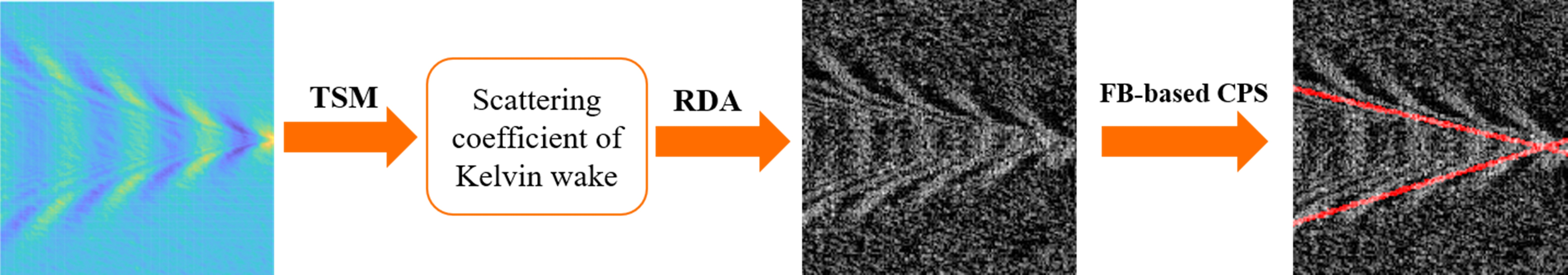
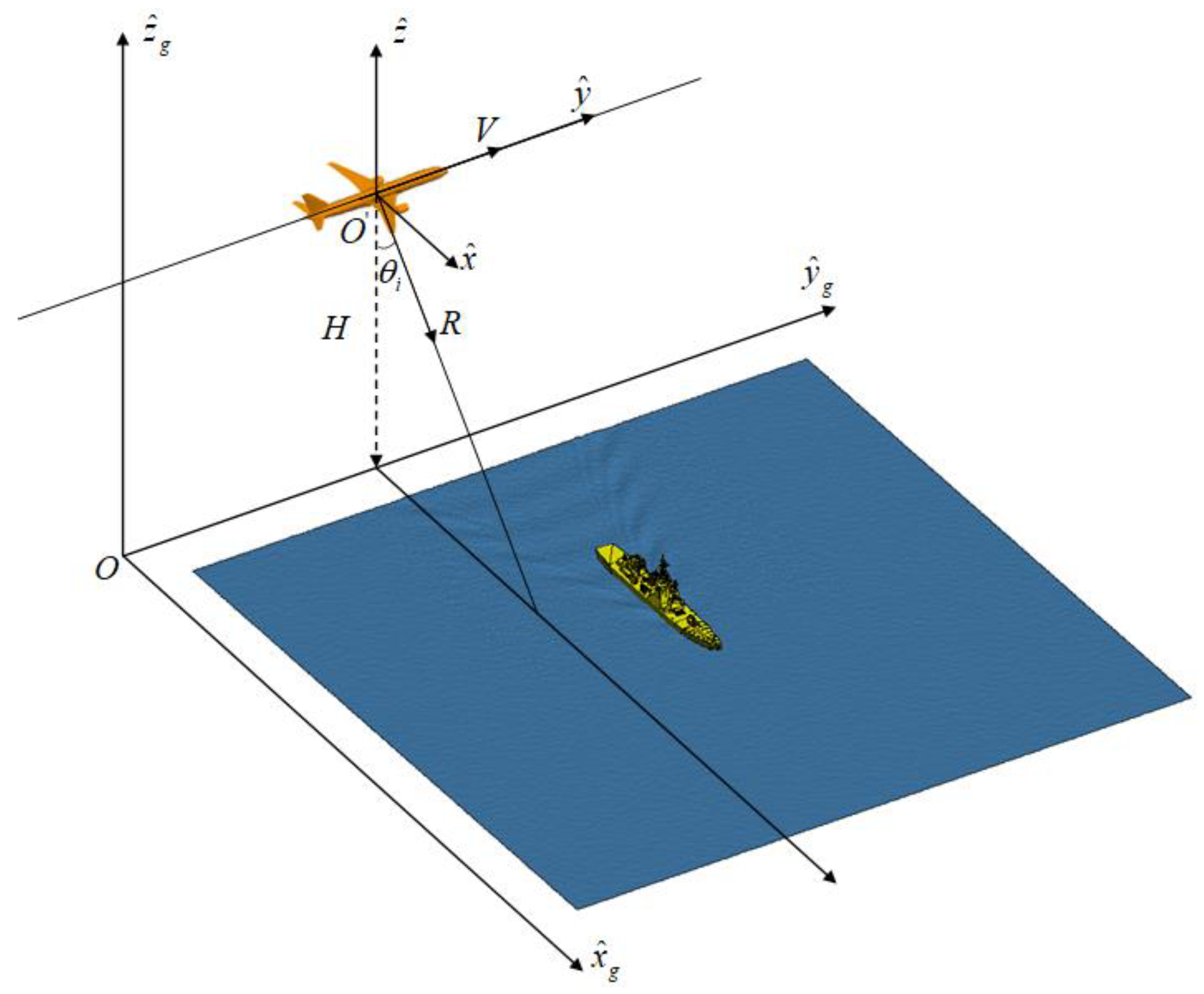
2. Kelvin Wake Modeling

Lord Kelvin presented the principle of water waves by moving ships in 1887. He described the ship as an ideal point perturbation with a Kelvin wake that contains two distinct waveforms, that is, transverse waves and divergent waves. The included angle between the divergent waves and transverse waves is between 16 ° and 19.5 ° . In this area, the divergent and transverse waves interfere with each other to form a cusp wave, thus forming the Kelvin arms.
It is assumed that the ship travels along the negative X-axis with velocity U s . The wave height of the Kelvin wake can be obtained from the superposition of the waves [17,22]:
ς ( x , y ) = Re π / 2 π / 2 A ( θ K ) exp [ i k r   sec 2 θ K ( x cos θ K + y sin θ K ) ] d θ K
where x and y represent the coordinates of the ship wake on the X-axis and Y-axis, respectively. k K sec 2 θ K ( x cos θ K + y sin θ K ) is the phase function and k K sec 2 θ K is the wavenumber of the wave component propagating along the angles of wave propagation θ K with the X-axis. A ( θ K ) is a function of a ship’s parameters. When the depth of water is limited, k K = g / U s 2 tanh ( k H ) , where k is the wavenumbers; when ( H ) , k K = g / U s 2 . The wavelength is λ m = 2 π / k K .
A ( θ K ) is usually described by the Michell thin ship theory [21], which holds that the water flow around a ship is generated by sources in the central plane of the ship and that the strength of the headwaters is proportional to the local slope of the ship, i.e.,
A ( θ K ) = 4 k K U s ( sec 3 θ K ) H ( k K sec 2 θ K , θ K )
H ( K , θ K ) = S H σ ( x , y , z ) exp ( K ( i x cos θ K + i y sin θ K + z ) ) d x d y
where H ( K , θ K ) is the Kochin function. The headwater intensity σ ( x , y , z ) can be written as follows:
σ ( x , y , z ) = 2 U s 4 π x f ( x , z )
If the hull shape f is parabolic, then
f ( x , z ) = { b ( 1 x 2 / l 2 )                 ( d < z < 0 , l < x < l ) 0             ( z < d )
where b is half of the ship’s breadth, l is the ship’s length, and d is the depth of immersion.
Therefore, the wave height of the Kelvin wake can be written as follows:
ς ( x , y ) = ς 0 ( x + l , y ) + C ς 0 ( x l , y ) + ς 1 ( x + l , y ) C ς 1 ( x l , y )
where C is the viscosity coefficient.
ς 0 ( x , y ) = 4 b π k K l π / 2 π / 2 ( 1 e k K d sec 2 θ K ) sin [ k K sec 2 θ K ( x cos θ K + y sin θ K ) ] d θ K
ς 1 ( x , y ) = 4 b π k K 2 l 2 π / 2 π / 2 cos θ K ( 1 e k K d sec 2 θ K ) sin [ k sec 2 θ K ( x cos θ K + y sin θ K ) ] d θ K
We illustrate the algorithm with a numerical example. The rough sea surface is simulated using the Elfouhaily-type wave spectrum [23]. Figure 3 depicts the composite scene of the rough sea surface and ship’s Kelvin wake at different ship speeds, ship azimuth angles, and viscosity coefficients. The ship’s length is l = 137.202   m , half of the ship’s breadth is b = 8.31   m , and the depth of immersion is d = 8.732   m . The size of the rough sea surface is 256   m × 256   m , the windspeed is 5   m / s , and the wind direction is 0 ° ; other parameters are shown in Table 1.

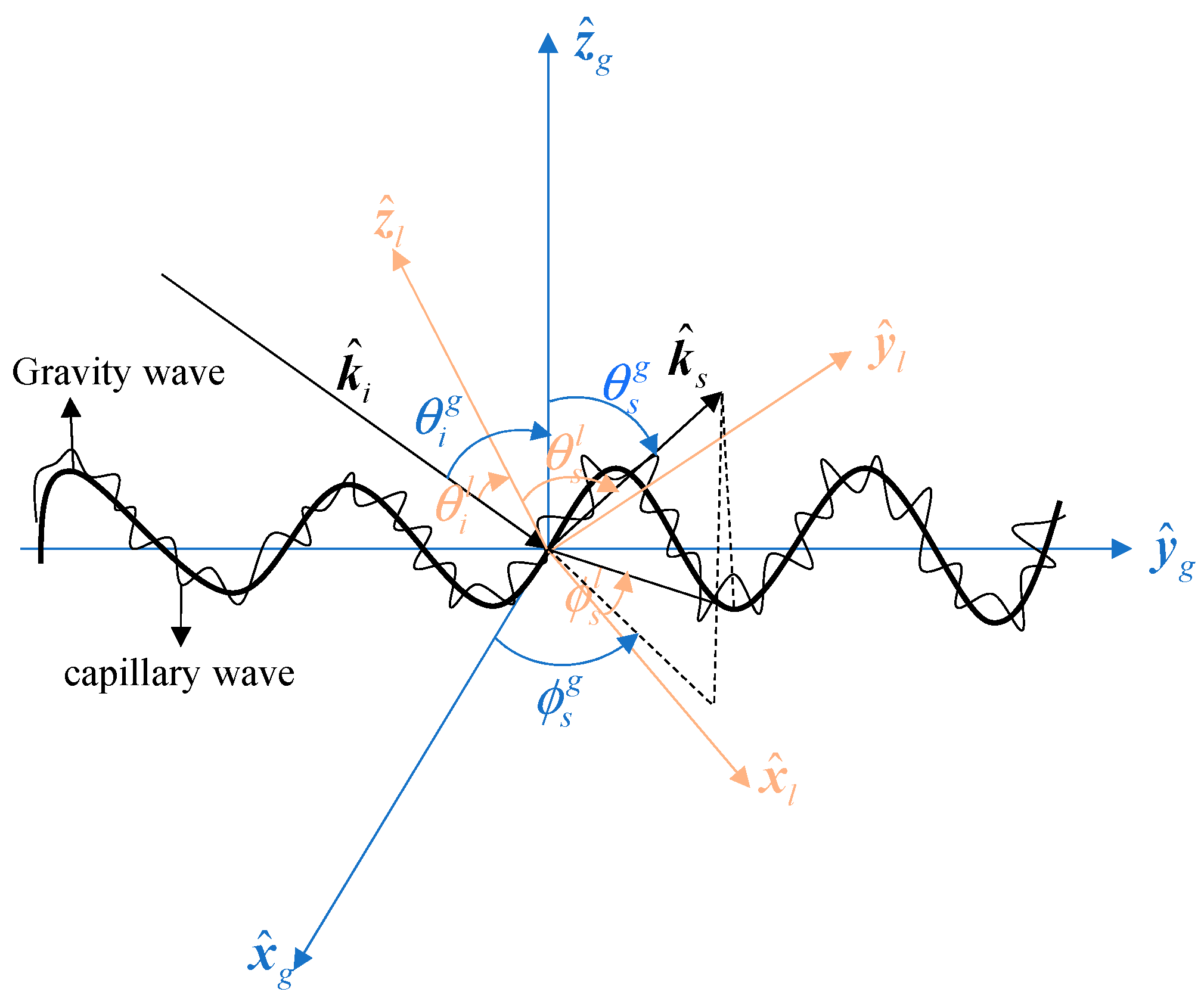
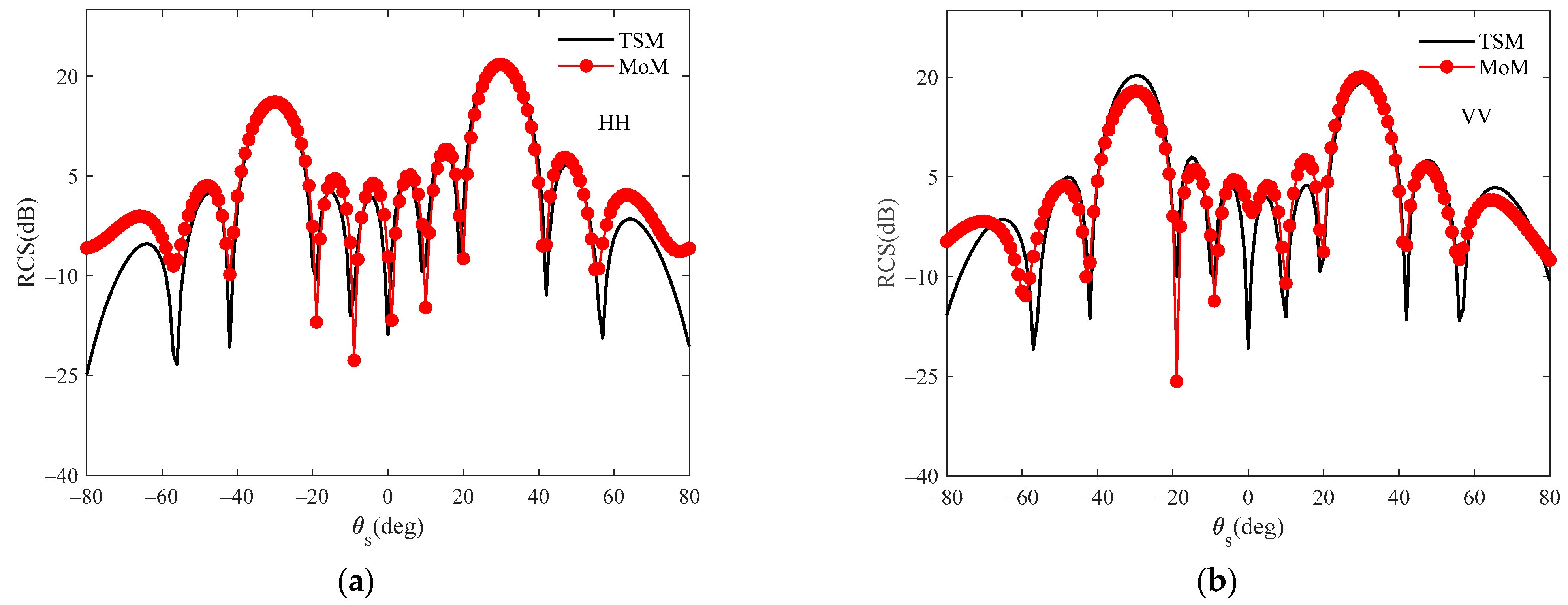
3. Scattering from a Dielectric Two-Scale Profile

Based on the two-scale sea surface model, the sea surface is visualized as a profile that is broken down by the number of slightly rough facets, with capillary waves as microscopic random roughness [24,25], as shown in Figure 4. When the EM waves are incident nearly vertically on the sea surface, the mirror reflection from the flat surface of the large-scale gravity waves is the main scattering mechanism in this incident interval. In this mechanism, the commonly used scattering model is the Kirchhoff approximation model (KAM), which can be expressed as [26]
σ p q K A M ( k ^ i , k ^ s ) = π k 2 | q | 2 q z 4 | F ˜ p q K A M | P ( z x tan , z y tan )
where q = k ( k ^ s k ^ i ) , k ^ i and k ^ s are the combined vectors of the incident and scattered wavenumbers, respectively, k is the number of EM waves, P ( z x tan , z y tan ) is the joint probability density function obeyed by z x tan and z y tan . z x tan = q x / q z and z y tan = q y / q z are the slopes of the tangent planes of the mirror points, and the polarization factor of KAM F ˜ p q K A M can be expressed as
F ˜ v v K A M = M 0 [ R v ( θ i l ) ( V ^ s k ^ i ) ( V ^ i k ^ s ) + R h ( θ i l ) ( H ^ s k ^ i ) ( H ^ i k ^ s ) ] F ˜ v h K A M = M 0 [ R v ( θ i l ) ( V ^ s k ^ i ) ( H ^ i k ^ s ) R h ( θ i l ) ( H ^ s k ^ i ) ( V ^ i k ^ s ) ] F ˜ h v K A M = M 0 [ R v ( θ i l ) ( H ^ s k ^ i ) ( V ^ i k ^ s ) R h ( θ i l ) ( V ^ s k ^ i ) ( H ^ i k ^ s ) ] F ˜ h h K A M = M 0 [ R v ( θ i l ) ( H ^ s k ^ i ) ( H ^ i k ^ s ) + R h ( θ i l ) ( V ^ s k ^ i ) ( V ^ i k ^ s ) ]
Here, θ i l is the local incidence angle. { k ^ i , k ^ s } and { H ^ i , H ^ s , V ^ i , V ^ s } are the incident and scattering unit vectors of the EM wave and its corresponding polarization unit vector, respectively. M 0 = | q | | q z | / { [ ( H ^ s k ^ i ) 2 + ( V ^ s k ^ i ) 2 ] k q z } . R v and R h are the Fresnel reflection coefficients corresponding to horizontal and vertical polarizations, respectively, and they can be expressed as
R v = ( ε cos θ i l ε sin 2 θ i l ) / ( ε cos θ i l + ε sin 2 θ i l )
R h = ( cos θ i l ε sin 2 θ i l ) / ( cos θ i l + ε sin 2 θ i l )
where ε is the dielectric constant of the ocean from the Debye model [27].
The scattering coefficient of an arbitrarily tilted micro-rough small surface element can be written as follows [26]:
σ p q T S P M ( k ^ i , k ^ s ) = 1 2 π k 2 | ε 1 | 2 | F ˜ P Q | 2 S ζ ( q l )
where S ζ ( q l ) is the spatial power spectrum [26]. F ˜ P Q denotes the polarization factor in the global coordinate system and can be written as follows:
[ F ˜ V V F ˜ V H F ˜ H V F ˜ H H ] = [ V ^ s v ^ s H ^ s v ^ s V ^ s h ^ s H ^ s h ^ s ] [ F v v F v h F h v F h h ] [ V ^ i v ^ i V ^ i h ^ i H ^ i v ^ i H ^ i h ^ i ]
where F p q is the polarization vectors and { H ^ i , V ^ i , H ^ s , V ^ s } and { h ^ i , v ^ i , h ^ s , v ^ s } are the incident and scattering unit vectors of the electromagnetic wave and its unit polarization vectors in the global and local coordinate systems, respectively. Their relationship can be written as follows:
H ^ i = ( H ^ i v ^ i ) v ^ i + ( H ^ i h ^ i ) h ^ i ,                         V ^ i = ( V ^ i v ^ i ) v ^ i + ( V ^ i h ^ i ) h ^ i H ^ s = ( H ^ s v ^ s ) v ^ s + ( H ^ s h ^ s ) h ^ s ,             V ^ s = ( V ^ s v ^ s ) v ^ s + ( V ^ s h ^ s ) h ^ s
Details of these are described elsewhere [26] and in our previous work [24,25].
In Figure 5, the bistatic scattering of the cosine surface is calculated by the method of moment (MoM) and TSM. The frequency of the incident wave is f = 2   GHz . The dielectric constant of the cosine surface is ε = ( 71.603 ,   50.657 ) . The incident angles are θ i g = 30 ° ϕ i g = 0 ° . The size of the cosine surface is 6λ × 6λ. As shown in Figure 5, the results of the TSM agree well with the results of the MoM. Therefore, the TSM is effective.

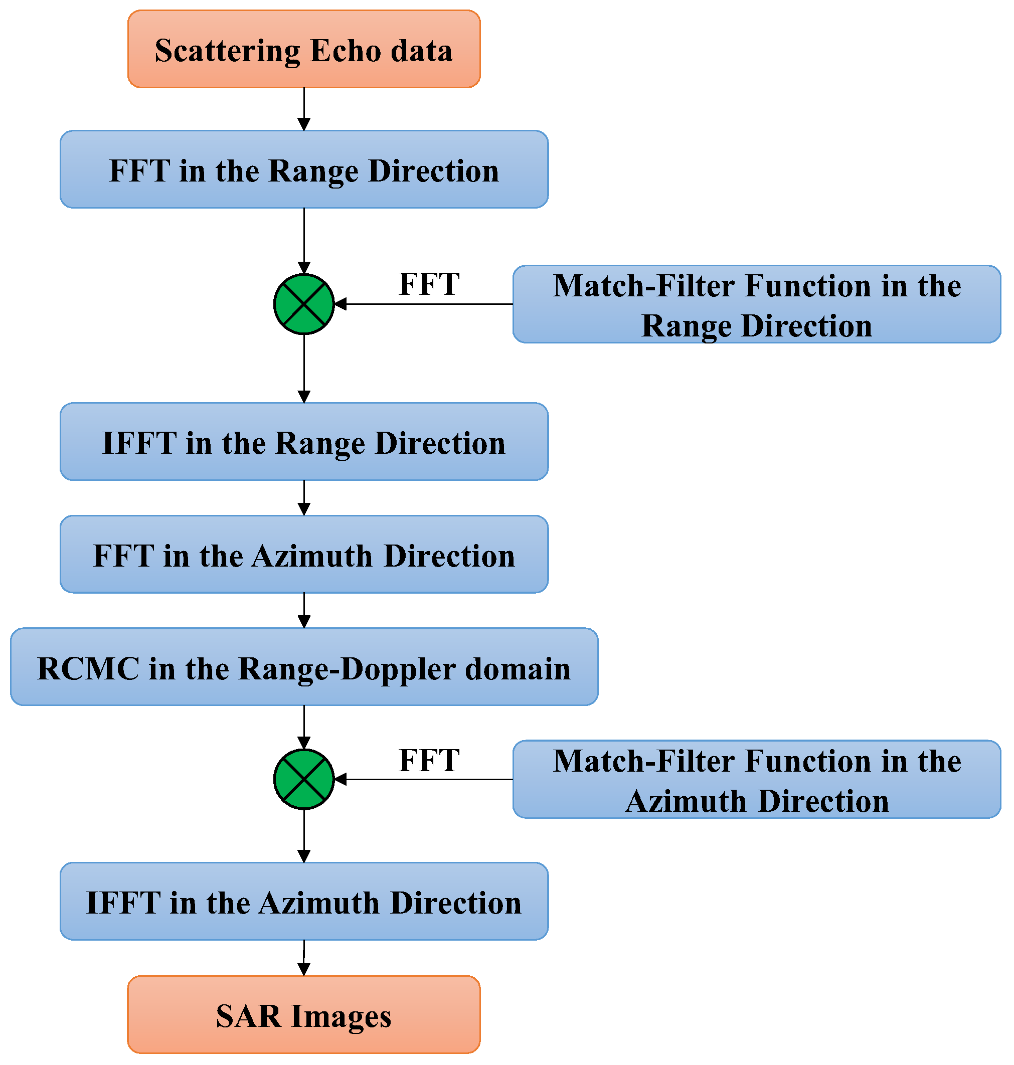
4. Range–Doppler Algorithm

The RDA [28] was used to simulate the Kelvin wake in SAR images in this paper. This algorithm consists of three main steps: range compression, range cell migration correction (RCMC), and azimuth compression. Range compression contains fast Fourier transform (FFT) in the range direction and inverse fast Fourier transform (IFFT) in the range direction; the azimuth compression is achieved by the IFFT in the azimuth direction. A detailed flow of the RDA is shown in Figure 6. With this algorithm, the scattering echo data obtained by the TSM are processed to obtain the Kelvin wake in SAR images.
We verified the results of numerically simulated SAR images by comparing real SAR data from satellite platforms, namely, TerraSAR-X [29], with simulated SAR images. The diagram of ship wake SAR imaging is shown in Figure 7. We identified the wake of the “TSX_20191128T052044.652_Vesuv_C414_O093_D_R_SM003_SSC” data in TerraSAR-X, and its latitude and longitude information is shown in Figure 8. The sea state and ship parameters of the real SAR data are not clear. Therefore, when simulating the Kelvin wake in SAR images, the parameters are arbitrarily selected. In the following case, the SAR platform velocity is V = 100 m/s, the platform altitude is H = 3000 m, the SAR resolution in the range and azimuth direction are both 0.5 m, the size of the illuminated area in the SAR images is 256 m in the range direction and 256 m in the azimuth direction, and the SAR integration time is 1 s. The wind speed is U = 3   m / s , the wind direction is 0 ° , and the ship’s speed is U s = 26   m / s . The corresponding result of the numerically simulated SAR image is shown in Figure 9.
Moreover, the perceptual hash algorithm [30] was used to calculate the similarity between real SAR data from TerraSAR-X and the result of the mathematically simulated SAR image, and the similarity reached 95.31%. Figure 10 depicts the “fingerprint” information of the two images in Figure 9 and reflects the similarity of the two images in Figure 9.
According to Figure 9 and Figure 10, the real SAR data from TerraSAR-X have the same characteristics as the results of the mathematically simulated SAR image. The accuracy of the simulation results is further verified.

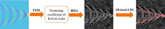
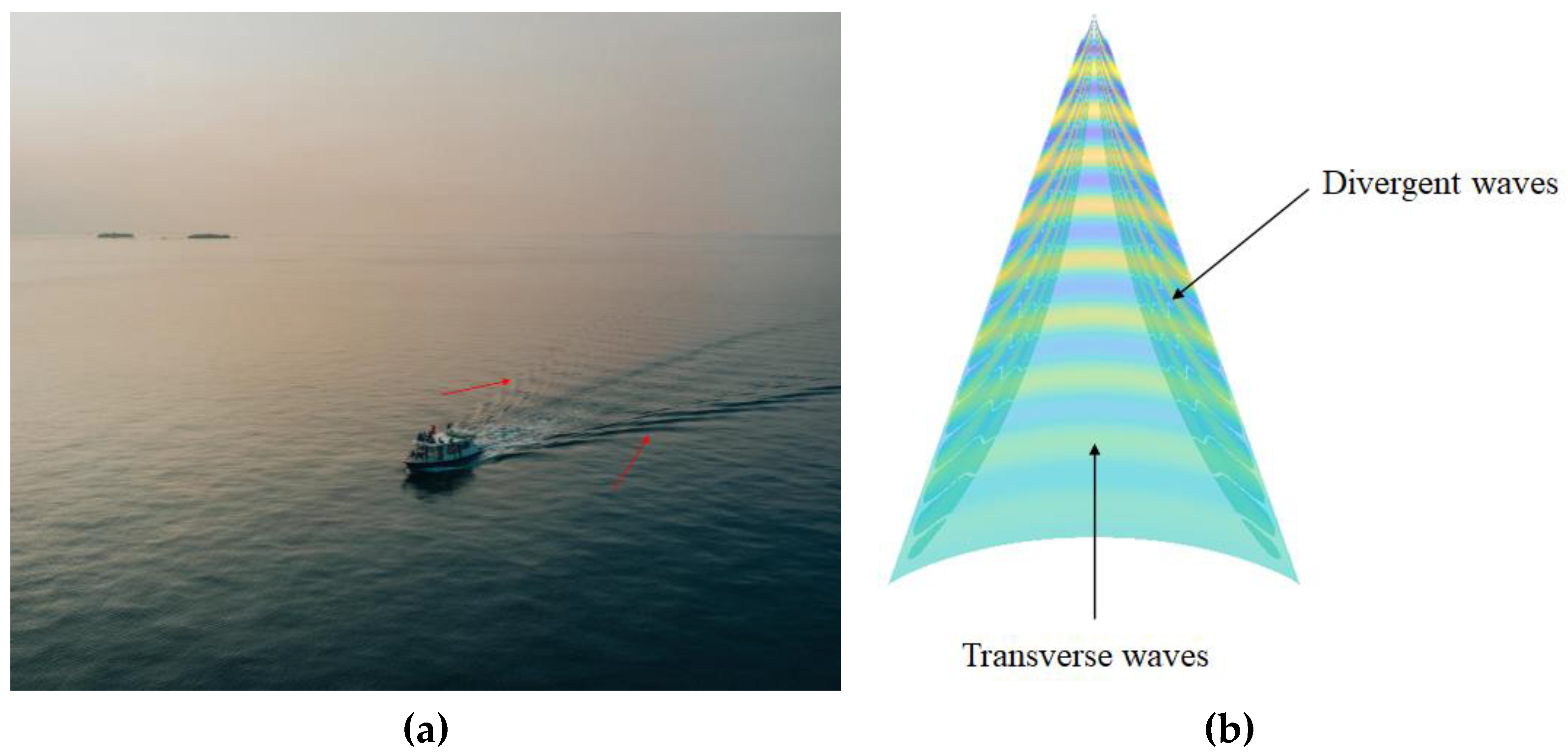
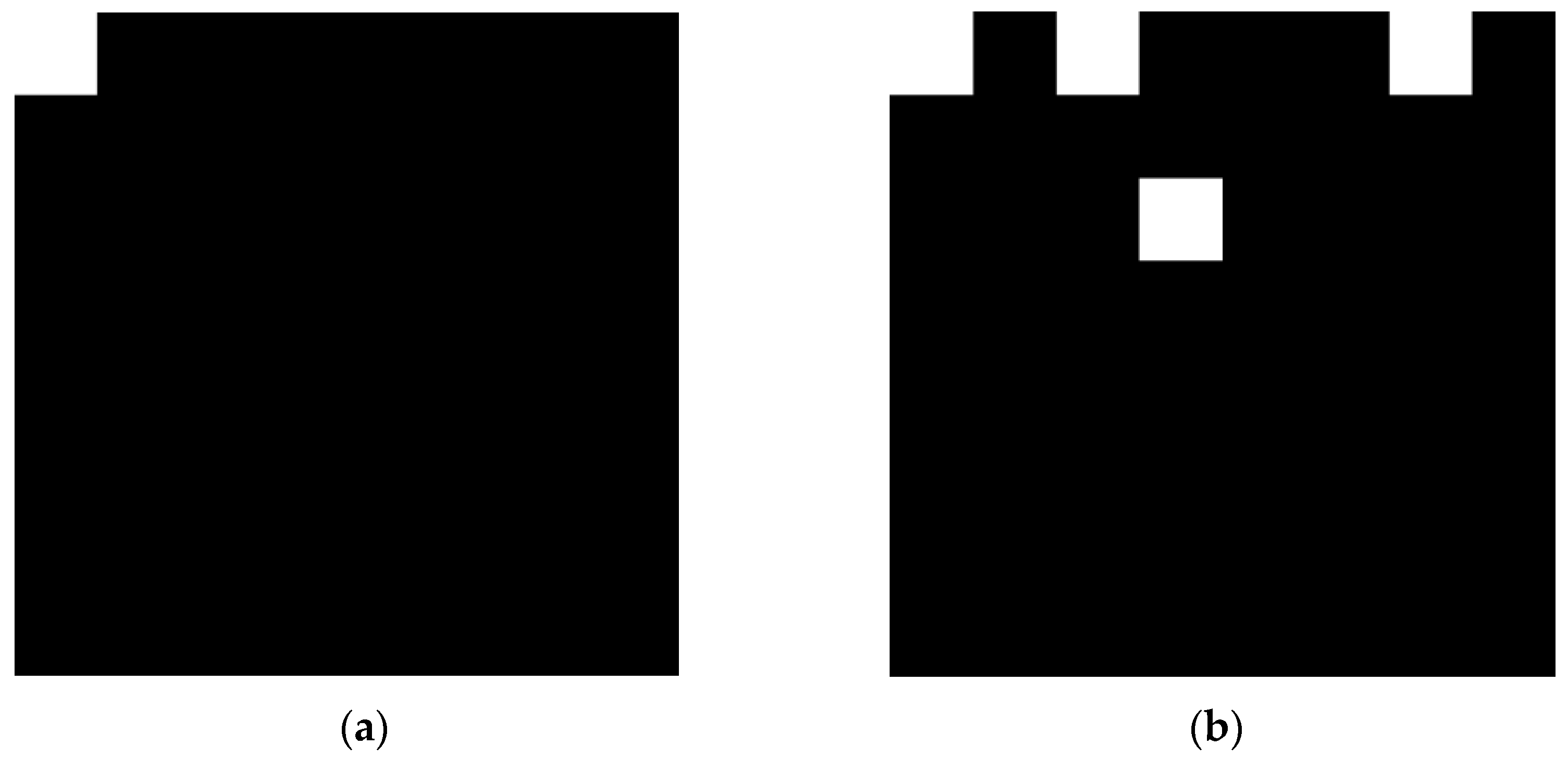
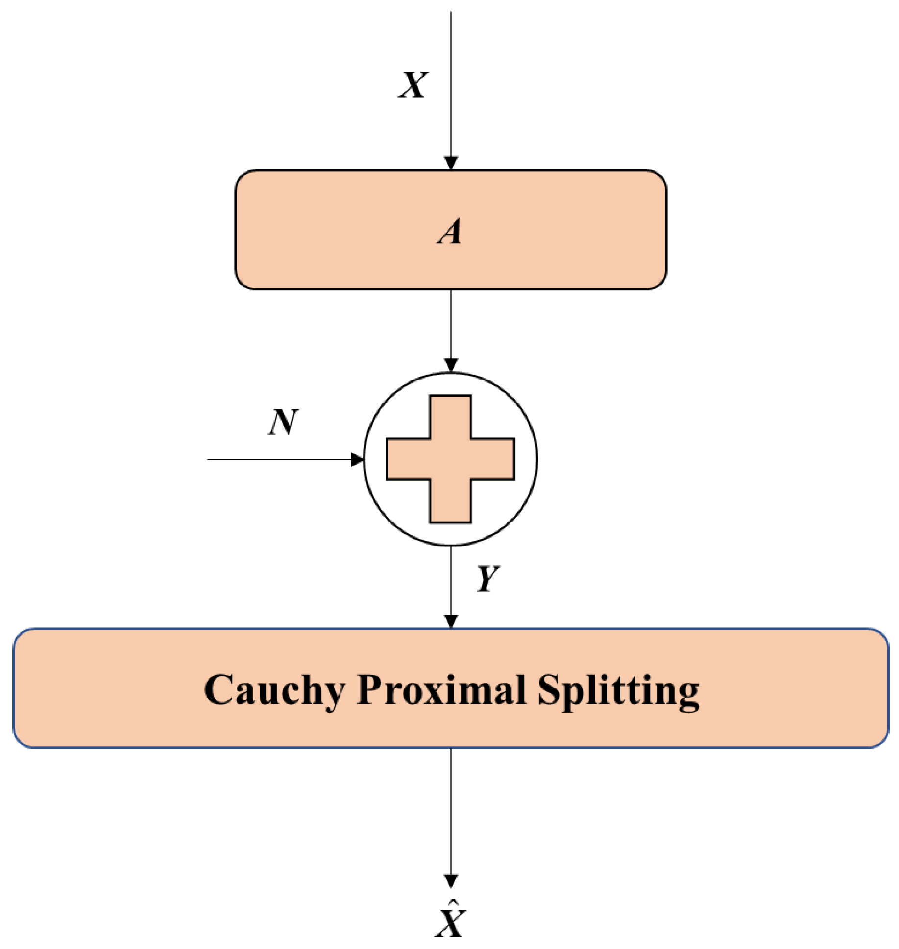
5. Inverse Problems of Kelvin Wake Detection in Numerically Simulated SAR Images

Since the ship wakes are modeled as linear features, the Radon transform maps straight lines in the original image space to points (line integral values) in ( ρ , θ ) space. Straight lines with high gray values in the image will form bright spots in ( ρ , θ ) space, while line segments with low gray values will form dark spots in ( ρ , θ ) space. Thus, the detection of straight lines can be translated into the detection of bright spots and dark spots in the transformed region. Therefore, the formation of a SAR image can be written in terms of its Radon transform as [30]
Y = A X + N
where Y is the SAR image. X ( ρ , θ ) is the image in the Radon domain. N refers to the additive noise, and the operator A = R 1 represents the inverse Radon transform. X ( ρ , θ ) represents the distance r from the center of Y and the orientation θ from the horizontal axis of Y .
In image processing applications, computing an integral of the intensities of image Y ( i , j ) over the hyperplane, which is perpendicular to θ , leads to Radon transform X ( ρ , θ ) of the given image Y . It can also be defined as a projection of the image along the angles, θ . Hence, for a given image Y , the general form of the Radon transform ( X = R Y = A T Y ) is
X ( r , θ ) = 2 Y ( i , j ) δ ( r i cos θ j sin θ ) d i d j
where δ ( ) is the Dirac delta function.
The inverse Radon transform Y = A X of the projected image X can be obtained from the filtered back projection algorithm [31] as
g ( r , θ ) = F 1 [ | υ | F [ X ( r , θ ) ] ] Y ( i , j ) = 0 π g ( r , θ ) δ ( r i cos θ j sin θ ) d r d θ
where υ is the radius in Fourier transform and F [ ] and F 1 [ ] refer to the forward and inverse Fourier transforms, respectively.
Since recovering the object of interest X from the observation Y is an ill-posed problem, we must consider prior information on X to obtain a stable and unique reconstruction result. Under the assumption of an independent and identically distributed (iid) Gaussian noise case, we express the data fidelity term ψ ( ) (i.e., the likelihood) as [20]
ψ ( Y , A X ) = Y A X 2 2 2 σ 2
where σ refers to the standard deviation of the noise. Having the prior knowledge p ( X ) , the problem of estimation X from the observed SAR image Y by using the signal model in (16) turns into a minimization problem [20]
X ^ = arg     min X     F ( X ) = arg     min X { Y A X 2 2 2 σ 2 log p ( X ) }
where we define ψ ( X ) = log p ( X ) as the penalty function, and F ( X ) = ψ ( Y , A X ) + ψ ( X ) is the cost function. As discussed earlier, the selection of ψ ( X ) (or equivalently p ( X ) ) plays a crucial role in estimating X in order to overcome the ill-posed problem and obtain a stable solution.
The Cauchy distribution is in the form of a nonconvex penalty for the purpose of solving imaging inverse problems. The Cauchy distribution is one of the special members of the α stable distribution family, which is known to be heavy-tailed and promote sparsity in various applications. Contrary to the general α stable family, it has a closed-form probability density function, which is given by [32]
p ( X ) α γ γ 2 + X 2
where γ is the scale parameter, which controls the spread of the distribution. By replacing p ( X ) in (16) with the Cauchy prior given in (21), we have [20]
X ^ Cauchy = arg min X Y A X 2 2 2 σ 2 i , j log ( γ γ 2 + X i , j 2 )
which is the Cauchy regularized minimization in X , with the cost function being Y A X 2 2 2 σ 2 log p ( X ) , and with the proposed nonconvex Cauchy-based penalty function [20]
ψ ( x ) = log ( γ γ 2 + x 2 )
The solution flow of inverse problems of Kelvin wake detection in numerically simulated SAR images is shown in Figure 11. Details of the proposed methodology are described elsewhere [33]. Based on [20], the FB-based CPS method is used to solve problems (22).

6. Results and Discussion

6.1. Influence of Various SAR System Parameters on Kelvin Wake Detection in Numerically Simulated SAR Images

6.1.1. Influence of Various Polarization on Kelvin Wake Detection in Numerically Simulated SAR Images

In Figure 12, the influence of different polarizations on Kelvin wake detection in numerically simulated SAR images at the X-band is compared, including horizontal–horizontal polarization (HH), vertical–vertical polarization (VV), VH polarization, and HV polarization. The azimuth and pitch angle are 90 ° and 60 ° , respectively. The wind speed is U = 1   m / s . The wind direction is 0 ° . The ship azimuth angle is 0 ° . The ship’s speed is U s = 6   m / s . The SAR integration time is 1 s.
As can be seen from Figure 12, the simulation results of HH (Figure 12a), VV (Figure 12b), and HV (Figure 12d) all reflect the characteristic of the Kelvin wake in SAR images, while Figure 12a is clearer. Moreover, the characteristics of Kelvin wake in SAR images can hardly be seen under the VH polarization. In the same scene, the SAR images with the same polarization are more sensitive to the waves whose propagation direction is parallel to the radar look direction, while SAR images with the cross-polarization have the opposite characteristic. Therefore, SAR should select one or more suitable observation angles according to the actual direction of the main waves. In conclusion, the imaging effect is better with HH polarization, and the characteristic of the Kelvin wake in SAR images is also easier to detect.

6.1.2. Influence of Different Pitch Angles on Kelvin Wake Detection in Numerically Simulated SAR Images

The pitch angle also affects the effective roughness of a rough sea surface with a Kelvin wake. According to the Rayleigh criterion [34], the roughness of a rough sea surface with a Kelvin wake decreases with an increase in the pitch angle. Therefore, the scattering echo energy decreases with an increase in the pitch angle.
In Figure 13, the influence of different pitch angles on Kelvin wake detection in numerically simulated SAR images is compared. The azimuth angle is 90 ° , and the pitch angles are 0 ° , 60 ° , and 90 ° , respectively. Other parameters are consistent with Figure 12. As can be seen from Figure 13, the scattering echo of a rough sea surface with a Kelvin wake decreased with an increase in the pitch angle. Moreover, the diffusion and transverse waves of the Kelvin wake in the SAR images first became clearer and then weaker. This is because the effective roughness of a rough sea surface with a Kelvin wake at a small pitch angle ( θ = 0 ° 20 ° ) is relatively small, which results in mirror reflections from the surface of large-scale gravity waves, in which case the main contribution is the scattering echo of the large-scale gravity waves. The diffuse echo of a rough sea surface plays a major role at a moderate pitch angle ( θ = 20 ° 70 ° ) for low sea states. Many experiments show that the Bragg resonance phenomenon occurs due to small-scale capillary waves and EM waves in the diffuse scattering region. Since the SAR can only detect the Bragg waves in the look direction, the Bragg scattering is the main scattering contribution in this case, and the characteristic of the Kelvin wake in SAR images can be clearly detected by SAR. Moreover, the white crown, cusp waves, and breaking waves play an important role at θ > 60 ° . The backscattering shows spikes, and speckles appear in the SAR images. Therefore, the difference between the sea surface background and the Kelvin wake waves in the SAR images is more obvious at large pitch angles, which makes the Kelvin wake in the SAR images clearer and easier to detect at large incidence angles.

6.1.3. Influence of Various Wavebands on Kelvin Wake Detection in Numerically Simulated SAR Images

The influence of various wavebands for Kelvin wake detection in simulated SAR images mainly has two aspects. One is the effective roughness of the rough sea surface, which mainly affects the scattering direction distribution of EM waves from the rough sea surface and further affects the echo energy. The other is their effect on the complex permittivity of the rough sea surface, which affects the reflection ability of the rough sea surface and the penetration ability of EM waves [35]. According to [36], the echo intensity increases as the radar wavelength decreases. Therefore, when other parameters remain unchanged, imaging the rough sea surface in different wavebands results in different echo intensities; as a result, the SAR image intensity data and texture also change greatly.
In Figure 14, the influence of the L-band, C-band, and X-band on Kelvin wake detection in numerically simulated SAR images is compared. The bandwidths are both 300 MHz. The pitch angle is 0 ° . Other parameters are consistent with Figure 12. As can be seen from Figure 14, the Kelvin wake in the SAR image is hardly visible in the L-band. The Kelvin wake in the SAR image can be observed at the C-band and X-band. Moreover, the Kelvin wake in the SAR image is detected only in the X-band. This is because the pitch angle is 0°, equivalent to looking down at the Kelvin wake. Since the capillary waves are sensitive to the wavelength of EM waves, when the wavelength is long, the corresponding effective roughness of the Kelvin wake is small. Therefore, the characteristics of the Kelvin wake are not easy to detect. On the contrary, the details and characteristics of the Kelvin wake in SAR images are more obvious. Therefore, the scattering echo in the X-band is more sensitive to rough sea surface changes at 0 ° pitch angles.
However, when there is an inclination angle between the direction of the EM wave incidence and the facets of the rough sea surface, the Kelvin wake was detected at either waveband. The influence of the wavelength on Kelvin wake detection in numerically simulated in SAR images with pitch angles of 0 ° , 60 ° and 90 ° , as shown in Table 2. Other parameters are consistent with Figure 12. It can be seen from the table that the EM waves are incident at 60 ° or 90 ° , i.e., the surface is illuminated at an inclined angle, and the Kelvin wake was detected at either waveband. This is because there is an inclination angle between the direction of the EM wave incidence and the facets of a rough sea surface increase the effective roughness of the rough sea surface, which leads to relatively large amplitude variations in the scattering echoes at the facet with larger wave slopes, which in turn highlights the texture of the Kelvin wake in SAR images. Therefore, it is appropriate to choose the X-band to study the detection of a Kelvin wake in numerically simulated SAR images.

6.2. Influence of Various Ship Parameters on Kelvin Wake Detection in Numerically Simulated SAR Images

According to Section 6.1, Kelvin wakes were more easily detected at the HH polarization, with a large pitch angle, and with the X-band. Therefore, HH polarization, a large pitch angle, and the X-band were chosen to study the effect of ship parameters on Kelvin wake detection in numerically simulated SAR images.

6.2.1. Influence of Various Ship Speeds on Kelvin Wake Detection in Numerically Simulated SAR Images

In Figure 15, the influence of various ship speeds on Kelvin wake detection in numerically simulated SAR images is compared. The ship’s speeds are U s = 3   m / s (Figure 15a), U s = 6   m / s (Figure 15b), U s = 10   m / s (Figure 15c), and U s = 18   m / s (Figure 15d), respectively. The wind direction is 0 ° . The ship azimuth angle is 0 ° . The wind speed is U = 4   m / s . The azimuth and pitch angles are both 90 ° . The SAR integration time is 1 s. Simulations with the X-band are performed for HH.
As seen from the figure, the ship’s speed is small, and the wavelength of the Kelvin wake is shorter. As the ship’s speed increases, the wavelength and wave height of the Kelvin wake increase significantly, as does the modulation effect on the rough sea surface. Therefore, the Kelvin arms become increasingly prominent and easier to observe.
Figure 16 shows the Radon transform of Figure 15d. From Figure 15d and Figure 16, both Kelvin arms in the SAR images are detected. The dark spots and bright spots in Figure 16, marked by circles in the Radon domain, correspond to the one dark wake and one bright wake marked by two red lines drawn in Figure 15d. These are consistent with the information observed in the SAR image.
In summary, we can draw the following conclusions: when U = 4 m/s and U > 6 m/s, the texture features of the Kelvin wake in the SAR image are completely visible. Moreover, the wave heights of the Kelvin wakes are large in this case, which makes these wakes easier to detect.

6.2.2. Influence of Various Ship Azimuth Angles on Kelvin Wake Detection in Numerically Simulated SAR Images

In Figure 17, the Kelvin wake in numerically simulated SAR images and its detection results are presented with various ship azimuth angles. The ship’s speed is U s = 6   m / s . The ship azimuth angles are 0 ° , 90 ° , and 120 ° . The wind speed is U = 1   m / s . Other parameters are consistent with Figure 15. As seen from the figure, SAR is more sensitive to Kelvin wake propagating along the radar look directions. Therefore, the Kelvin wakes in numerically simulated SAR images are unsymmetric except for those perpendicular to and parallel to the radar motion direction. Moreover, the Kelvin arms in any ship’s azimuth angle were detected.
To comprehensively illustrate the influence of ship motion parameters on the size of the wake physical field, Table 3 describes the detection accuracy of the Kelvin wakes in numerically simulated SAR images when the wind speed and hull parameters are changed. The wind speed, ship’s speed, and ship azimuth angles are listed in the table, and other parameters are consistent with Figure 15. It can be seen from the table that the detection results of the ship Kelvin wake in simulated SAR images were the same for different ship azimuth angles. When U = 3   m / s and U s < 6   m / s , no wake was detected, and wakes are detected at all other ship speeds. When U = 6   m / s and U s < 8   m / s , the wake was not detected, nor could it be detected when U = 10   m / s and U s < 12   m / s .

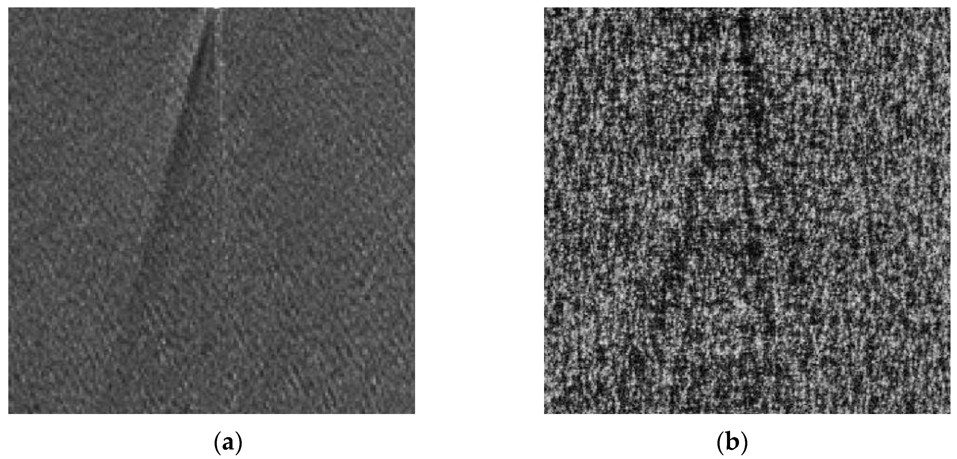
6.3. Influence of Noise on the Kelvin Wake in Simulated SAR Images

A jamming bomb is the necessary soft antimissile means on modern ships. After the jamming bomb explodes in the air, it ejects substantial chaff, which interferes with the radar seeker of the incoming missile. Based on this, we simulated the effect of actual jammers by adding noise to the numerically simulated SAR images. In this set of simulations, the SAR images were multiplied with gamma [37] noise sequences with a number of looks, L, chosen to be 5. As shown in Figure 18, the simulation parameters are consistent with those shown in Figure 15b. In Figure 19, U s = 11   m / s , U = 10   m / s , and the ship azimuth angle is 0°. As shown in Figure 18 and Figure 19, the characteristics of the Kelvin wakes in SAR images were disturbed by noise, and the ship wakes were not detected.
In addition, for the cases in Table 3, we combined them with gamma noise sequences and set L = 5. Notably, the detection results of the ship’s Kelvin wake were still the same for a different ship azimuth angle. When U = 3   m / s and U s < 7   m / s , the wake could not be detected, nor could it be detected when U = 6   m / s and U s < 9   m / s or when U = 10   m / s and U s < 13   m / s . Thus, the detection of ship wakes in SAR images was degraded in the presence of noise. On the other hand, these results show that ship wake stealth can be promoted by jamming.

7. Conclusions

This paper introduced a nonconvex regularization with a Cauchy-based penalty for discussing the influence of ship parameters and speckle noise in the numerically simulated SAR images. The TSM was used to obtain the EM scattering echoes of simulated Kelvin wakes. Then, the SAR images of Kelvin wakes were generated by RDA, and wakes were reconstructed in the Radon domain using the FB-based CPS algorithm. The results show that the Kelvin wakes were more easily detected in HH polarization with a large pitch angle and in the X-band. Based on this, the influence of ship parameters and speckle noise on the detection of ship wake in numerically simulated SAR images was discussed. In the absence of jamming bomb, when the wind speed is U = 3   m / s , the ship will not be detected if it keeps sailing at U s < 6   m / s , nor will it be detected when U = 6   m / s and U s < 8   m / s or when U = 10   m / s and U s < 12   m / s . In the case that the ship is protected by jamming bomb, when the wind speed is U = 3   m / s , the ship will not be detected if it keeps sailing at a speed below 7 m/s at this time, nor will it be detected when U = 6   m / s and U s < 9   m / s or when U = 10   m / s and U s < 13   m / s . These research conclusions are of value to the development of ship wake stealth technology and the improvement of ship safety.
The RDA in this paper is computationally intensive and may reduce the resolution of the imaging when performing RCMC. Therefore, in order to improve the resolution of SAR images, future investigations on this topic will focus on improved RDA for SAR imaging, such as secondary range compression (SRC) and squint imaging mode (SIM). Moreover, the TSM will be considered for acceleration using CUDA to improve computational efficiency.

Author Contributions

Conceptualization, J.W. and Y.W.; methodology, J.W. and Y.W.; validation, J.W., Y.W. and L.G.; investigation, J.W., S.C. and Y.W.; writing—original draft preparation, J.W.; funding acquisition, L.G. and Y.W. All authors have read and agreed to the published version of the manuscript.

Funding

This research was funded by the National Natural Science Foundation of China (Grant No.62231021, U21A20457, 61871457, and 61971338), the Foundation for Innovative Research Groups of the National Natural Science Foundation of China (Grant No.61621005) and the Natural Science Basic Research Program of Shaanxi (Grant No. 2023-JC-YB-537).

Data Availability Statement

Not applicable.

Conflicts of Interest

The authors declare no conflict of interest.

References

  1. Gong, M.; Cao, Y.; Wu, Q. A Neighborhood-Based Ratio Approach for Change Detection in SAR Images. IEEE Geosci. Remote Sens. Lett. 2012, 9, 307–311. [Google Scholar] [CrossRef]
  2. Hakim, W.L.; Achmad, A.R.; Eom, J.; Lee, C.-W. Land Subsidence Measurement of Jakarta Coastal Area Using Time Series Interferometry with Sentinel-1 SAR Data. J. Coast. Res. 2020, 102, 75–81. [Google Scholar] [CrossRef]
  3. Kang, M.S.; Kim, K.T. Automatic SAR Image Registration via Tsallis Entropy and Iterative Search Process. IEEE Sens. J. 2020, 20, 7711–7720. [Google Scholar] [CrossRef]
  4. Lyden, J.; Hammond, R.; Lyzenga, D.; Shuchman, R. Synthetic Aperture Radar Imaging of Surface Ship Wakes. J. Geophys. Res. 1988, 93, 12293–12303. [Google Scholar] [CrossRef]
  5. Wright, J. A new model for sea clutter. IEEE Trans. Antennas Propag. 1968, 16, 217–223. [Google Scholar] [CrossRef]
  6. Wright, J. Backscattering from capillary waves with application to sea clutter. IEEE Trans. Antennas Propag. 1966, 14, 749–754. [Google Scholar] [CrossRef]
  7. Del Prete, R.; Graziano, M.D.; Renga, A. First Results on Wake Detection in SAR Images by Deep Learning. Remote Sens. 2021, 12, 4573. [Google Scholar] [CrossRef]
  8. Ding, K.; Yang, J.; Wang, Z.; Ni, K.; Wang, X.; Zhou, Q. Specific Windows Search for Multi-Ship and Multi-Scale Wake Detection in SAR Images. Remote Sens. 2022, 14, 25. [Google Scholar] [CrossRef]
  9. Rey, M.T.; Tunaley, J.K.; Folinsbee, J.T.; Jahans, P.A.; Dixon, J.A.; Vant, M.R. Application of Radon Transform Techniques to Wake Detection in Seasat-A SAR Images. IEEE Trans. Geosci. Remote Sens. 1990, 28, 553–560. [Google Scholar] [CrossRef]
  10. Biondi, F. Low-Rank Plus Sparse Decomposition and Localized Radon Transform for Ship-Wake Detection in Synthetic Aperture Radar Images. IEEE Geosci. Remote Sens. Lett. 2018, 15, 117–121. [Google Scholar] [CrossRef]
  11. Biondi, F. A Polarimetric Extension of Low-Rank Plus Sparse Decomposition and Radon Transform for Ship Wake Detection in Synthetic Aperture Radar Images. IEEE Geosci. Remote Sens. Lett. 2019, 16, 75–79. [Google Scholar] [CrossRef]
  12. Graziano, M.D. SAR-based ship route estimation by wake components detection and classification. In Proceedings of the 2015 IEEE International Geoscience and Remote Sensing Symposium (IGARSS), Milan, Italy, 26–31 July 2015. [Google Scholar]
  13. Ai, J.; Qi, X.; Yu, W.; Deng, Y.; Liu, F.; Shi, L.; Jia, Y. A Novel Ship Wake CFAR Detection Algorithm Based on SCR Enhancement and Normalized Hough Transform. IEEE Geosci. Remote Sens. Lett. 2011, 8, 681–685. [Google Scholar] [CrossRef]
  14. Xu, Z.; Tang, B.; Cheng, S. Faint Ship Wake Detection in PolSAR Images. IEEE Geosci. Remote Sens. Lett. 2018, 15, 1055–1059. [Google Scholar] [CrossRef]
  15. Hennings, I.; Romeiser, R.; Alpers, W.; Viola, A. Radar imaging of Kelvin arms of ship wakes. Int. J. Remote Sens. 1999, 20, 2519–2543. [Google Scholar] [CrossRef]
  16. Tunaley, J.K.E.; Buller, E.H.; Wu, K.H.; Rey, M.T. The simulation of the SAR image of a ship wake. IEEE Trans. Geosci. Remote Sens. 1991, 29, 149–156. [Google Scholar] [CrossRef]
  17. Oumansour, K.; Wang, Y.; Saillard, J. Multifrequency SAR observation of a ship wake. IEE Proc. Radar Sonar Navig. 1996, 143, 275–280. [Google Scholar] [CrossRef]
  18. Zilman, G.; Zapolski, A.; Marom, M. On Detectability of a Ship’s Kelvin Wake in Simulated SAR Images of Rough Sea Surface. IEEE Trans. Geosci. Remote Sens. 2015, 53, 609–619. [Google Scholar] [CrossRef]
  19. Karakus, O.; Rizaev, I.; Achim, A. Ship Wake Detection in SAR Images via Sparse Regularization. IEEE Trans. Geosci. Remote Sens. 2020, 58, 1665–1677. [Google Scholar] [CrossRef] [Green Version]
  20. Karakuş, O.; Achim, A. On Solving SAR Imaging Inverse Problems Using Non-Convex Regularisation with a Cauchy-based Penalty. IEEE Trans. Geosci. Remote Sens. 2021, 59, 5828–5840. [Google Scholar] [CrossRef]
  21. Wehausen, J.V.; Laitone, E.V. Surface Waves. In Fluid Dynamics/Strömungsmechanik; Truesdell, C., Ed.; Springer: Berlin/Heidelberg, Germany, 1960; pp. 446–778. [Google Scholar]
  22. Kostyukov, A.A. Theory of Ship Waves and Wave Resistance; Effective Communications Inc.: Iowa City, IA, USA, 1968. [Google Scholar]
  23. Elfouhaily, T.; Chapron, B.; Katsaros, K.; Vandemark, D. A unified directional spectrum for long and short wind-driven waves. J. Geophys. Res. 1997, 102, 15781–15796. [Google Scholar] [CrossRef] [Green Version]
  24. Wei, Y.; Guo, L.; Li, J. Numerical Simulation and Analysis of the Spiky Sea Clutter from the Sea Surface with Breaking Waves. IEEE Trans. Antennas Propag. 2015, 63, 4983–4994. [Google Scholar] [CrossRef]
  25. Zhang, M.; Chen, H.; Yin, H.C. Facet-Based Investigation on EM Scattering from Electrically Large Sea Surface with Two-Scale Profiles: Theoretical Model. IEEE Trans. Geosci. Remote Sens. 2011, 49, 1967–1975. [Google Scholar] [CrossRef]
  26. Elfouhaily, T.M.; Guérin, C.-A. A critical survey of approximate scattering wave theories from random rough surfaces. Waves Random Media 2004, 14, R1–R40. [Google Scholar] [CrossRef]
  27. Debye, P. Polar Molecules; Chemical Catalog Co.: New York, NY, USA, 1929. [Google Scholar]
  28. Yulong, S.; Zhaoda, Z. Squint mode airborne SAR processing using RD algorithm. In Proceedings of the IEEE 1997 National Aerospace and Electronics Conference, NAECON 1997, Dayton, OH, USA, 14–17 July 1997; Volume 2, pp. 1025–1029. [Google Scholar] [CrossRef]
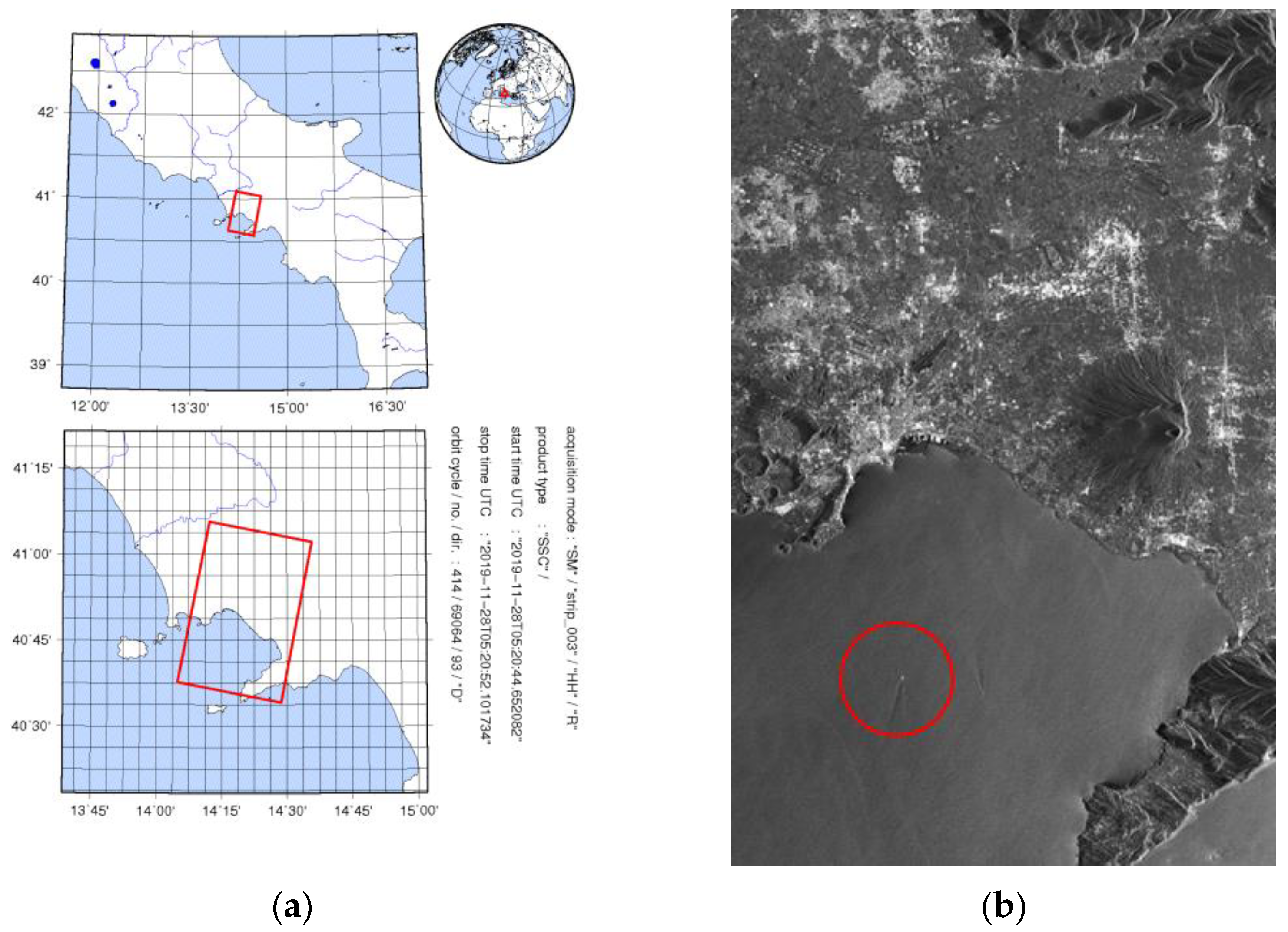
  29. Airbus Defence and Space, The TerraSAR-X Sample Products. Available online: https://www.intelligence-airbusds.com/en/ (accessed on 28 November 2019).
  30. Schneider, M.; Shih-Fu, C. A robust content based digital signature for image authentication. In Proceedings of the 3rd IEEE International Conference on Image Processing, Lausanne, Switzerland, 19 September 1996; Volume 223, pp. 227–230. [Google Scholar]
  31. Kak, A.C.; Slaney, M. Principles of Computerized Tomographic Imaging; Society for Industrial and Applied Mathematics: Philadelphia, PA, USA, 1988. [Google Scholar]
  32. Wan, T.; Canagarajah, N.; Achim, A. Segmentation of noisy colour images using Cauchy distribution in the complex wavelet domain. Image Process. IET 2011, 5, 159–170. [Google Scholar] [CrossRef]
  33. Kelley, B.T.; Madisetti, V.K. The fast discrete Radon transform. I. Theory. IEEE Trans. Image Process. 1993, 2, 382–400. [Google Scholar] [CrossRef] [Green Version]
  34. Peake, W.H.; Oliver, T.L. The Response of Terrestrial Surfaces at Microwave Frequencies; Ohio State University: Columbus, OH, USA, 1971. [Google Scholar]
  35. Shu, N. Principles of Microwave Remote Sensing; Wuhan University Press: Wuhan, China, 2003. [Google Scholar]
  36. Long, M.W. Radar Reflectivity of Land and Sea; Artech House: Norwood, MA, USA, 1983. [Google Scholar]
  37. Gagnon, L.; Jouan, A. Speckle Filtering of SAR Images-A Comparative Study Between Complex-Wavelet-Based and Standard Filters. Proc. SPIE 1997, 3169, 80–91. [Google Scholar] [CrossRef]
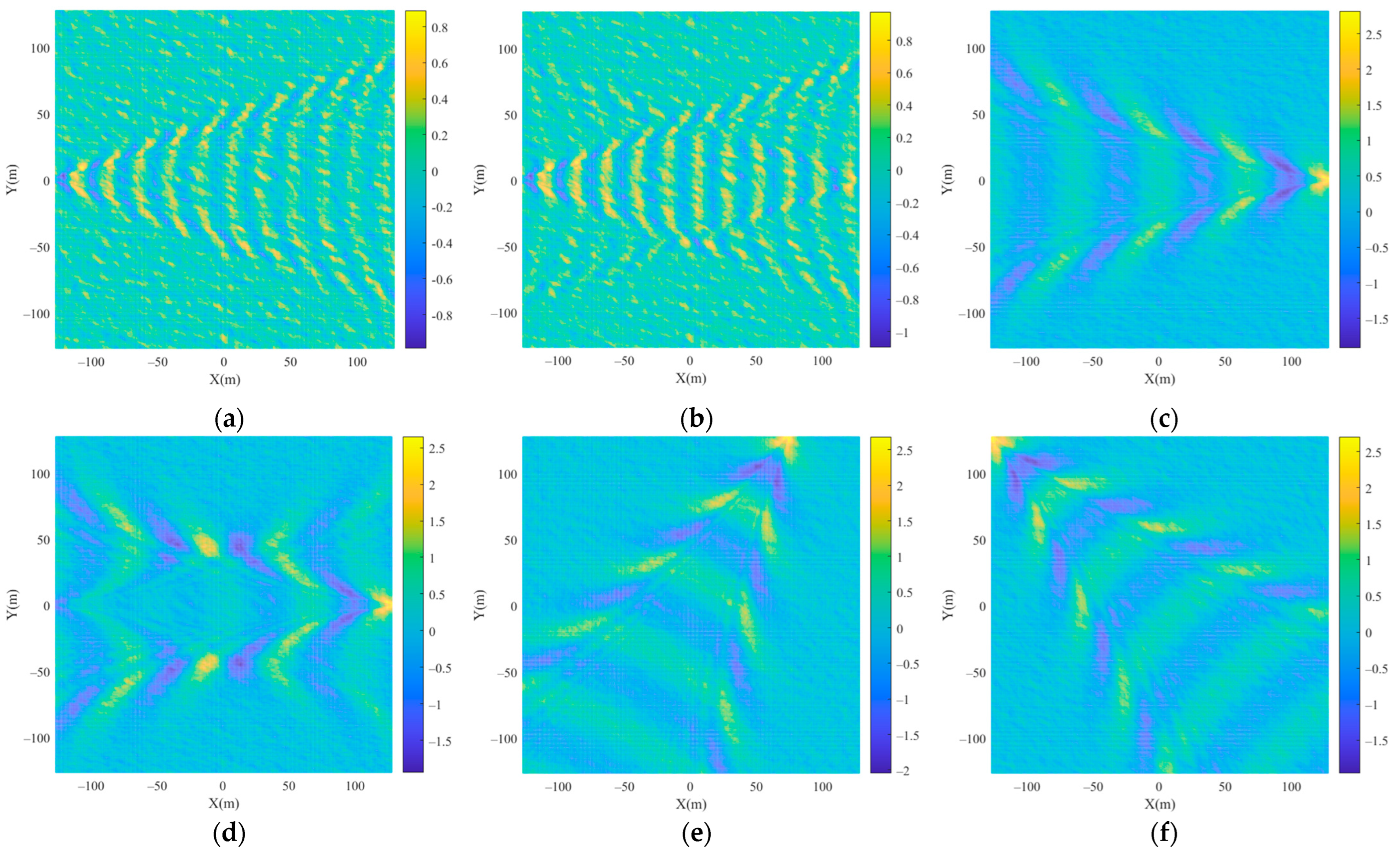
Figure 1. Kelvin wake. (a) Kelvin wake realistic view, the red arrows indicated the kelvin wake. (b) Kelvin wake model simulated.
Remotesensing 15 01089 g001
Figure 2. Flow diagram of Kelvin wake detection in SAR images.
Remotesensing 15 01089 g002
Figure 3. Composite scene of the rough sea surface and ship’s Kelvin wake at different ship speeds, ship azimuth angles, and viscosity coefficients. (a) U s = 6   m / s ,   φ s = 90 ° ,   C = 0 ; (b) U s = 6   m / s ,   φ s = 90 ° ,   C = 0.6 ; (c) U s = 10   m / s ,   φ s = 0 ° ,   C = 0 ; (d) U s = 10   m / s ,   φ s = 0 ° ,   C = 0.6 ; (e) U s = 10   m / s ,   φ s = 75 ° ,   C = 0 ; (f) U s = 10   m / s ,   φ s = 135 ° ,   C = 0 .
Remotesensing 15 01089 g003
Figure 4. Two-scale sea surface model. The global coordinate systems { x ^ g , y ^ g , z ^ g } are fixed on the Earth, whereas { x ^ l , y ^ l , z ^ l } is the local coordinate system fixed on the facet of the rough sea surface.
Remotesensing 15 01089 g004
Figure 5. Bistatic scattering of a cosine surface. (a) HH; (b) VV.
Remotesensing 15 01089 g005
Figure 6. Flowchart of the RDA.
Remotesensing 15 01089 g006
Figure 7. Ship wake SAR imaging model.
Remotesensing 15 01089 g007
Figure 8. Real SAR data information. (a) Latitude and longitude of “TSX_20191128T052044.652_Vesuv_C414_O093_D_R_SM003_SSC” data, the rectangle indicates the latitude and longitude information where the intercepted wake is located.; (b) SAR image, the circle indicates intercepted wake.
Remotesensing 15 01089 g008
Figure 9. Real SAR data from TerraSAR-X and the result of the numerically simulated SAR image (a) Real SAR data from TerraSAR-X; (b) Kelvin wake in the numerically simulated SAR image.
Remotesensing 15 01089 g009
Figure 10. Comparison of the similarity between the real SAR data from TerraSAR-X and the result of the numerically simulated SAR image. (a) Hash value of real SAR data from TerraSAR-X; (b) hash value of Kelvin wake in the numerically simulated SAR image.
Remotesensing 15 01089 g010
Figure 11. The solution flow of inverse problems of Kelvin wake detection in numerically simulated SAR images.
Remotesensing 15 01089 g011
Figure 12. Kelvin wake in the simulated SAR images at different polarizations and its detection results. (a) HH; (b) VV; (c) VH; (d) HV.
Remotesensing 15 01089 g012
Figure 13. Kelvin wake in the simulated SAR images at different pitch angles and its detection results (a) θ   =   0 ° ; (b) θ   =   60 ° ; (c) θ   =   90 ° .
Remotesensing 15 01089 g013
Figure 14. Kelvin wake in the simulated SAR images at various wavebands and its detection results. (a) L-band; (b) C-band; (c) X-band.
Remotesensing 15 01089 g014
Figure 15. Kelvin wake in the simulated SAR images and detection results at different speeds. (a) U s = 3   m / s ; (b) U s = 6   m / s ; (c) U s = 10   m / s ; (d) U s = 18   m / s .
Remotesensing 15 01089 g015aRemotesensing 15 01089 g015b
Figure 16. Radon transform of Figure 15d.
Remotesensing 15 01089 g016
Figure 17. Kelvin wake in numerically simulated SAR images and detection results at different ship azimuth angles. (a) φ s = 0 ° ; (b) φ s = 90 ° ; (c) φ s = 120 ° .
Remotesensing 15 01089 g017aRemotesensing 15 01089 g017b
Figure 18. Artificial interference detection of the Kelvin wake in SAR images ( U = 4   m / s ; U s = 6   m / s ). (a) Original image; (b) speckled image.
Remotesensing 15 01089 g018
Figure 19. Artificial interference detection of Kelvin wake in SAR images ( U = 10   m / s ; U s = 11   m / s ). (a) Original image; (b) speckled image.
Remotesensing 15 01089 g019
Table 1. Simulation parameters of Figure 3.
Figure U s  (m/s)Ship Azimuth AngleViscosity Coefficient
Figure 3a6 90 ° 0
Figure 3b6 90 ° 0.6
Figure 3c10 0 ° 0
Figure 3d10 0 ° 0.6
Figure 3e10 75 ° 0
Figure 3f10 135 ° 0
Table 2. Influence of wavelength on Kelvin wake detection in numerically simulated SAR images with different pitch angles.
Pitch AngleWavebandKelvin1Kelvin2
0 ° L××
C
X
60 ° L
C
X
90 ° L
C
X
The × indicates that the wake is not detected, and √ indicates the wake is detected.
Table 3. Detection accuracy of Kelvin wake in numerically simulated SAR images for different wind speeds and hull parameters.
Wind Speed (m/s)Ship Azimuth Angle U s (m/s) Kelvin1Kelvin2
3 90 ° 3××
5××
6
10
120 ° 3××
5××
6
10
6 90 ° 3××
6××
7×
10
120 ° 3××
6××
7×
10
10 90 ° 3××
6××
10××
11×
12
120 ° 3××
6××
10××
11×
12
The × indicates that the wake is not detected, and √ indicates the wake is detected.
Disclaimer/Publisher’s Note: The statements, opinions and data contained in all publications are solely those of the individual author(s) and contributor(s) and not of MDPI and/or the editor(s). MDPI and/or the editor(s) disclaim responsibility for any injury to people or property resulting from any ideas, methods, instructions or products referred to in the content.

