Article

Eddy Characteristics and Vertical Structure in the Bay of Bengal during Different Monsoon Regimes

by
Corinne B. Trott
1 and
Bulusu Subrahmanyam
2,*
1
Naval Research Laboratory, Stennis Space Center, Hancock County, MS 39529, USA
2
School of the Earth, Ocean, and Environment, University of South Carolina, Columbia, SC 29208, USA
*
Author to whom correspondence should be addressed.
Remote Sens. 2023, 15(4), 1079; https://doi.org/10.3390/rs15041079
Submission received: 13 January 2023 / Revised: 10 February 2023 / Accepted: 13 February 2023 / Published: 16 February 2023

Abstract

:
The evolution of mesoscale eddies in the Bay of Bengal (BoB) and their characteristics (number of eddies, radius, amplitude, and eddy kinetic energy) are addressed during all strong, normal, and weak monsoon regimes from 1993 to 2019. Their impacts on the 3–7-day synoptic oscillations of atmospheric precipitation and upper ocean heat content are also assessed. In the western Bay, eddies are located in the meandering East India Coastal Current (EICC). The propagation of coastally trapped Kelvin waves into the Andaman Sea varies with monsoon intensity. Eddies with smaller radii, weaker amplitudes, increased vertical mixing, and deeper vertical extents were found during weak monsoons. Eddy kinetic energy (EKE) of EICC anticyclonic eddies is high (1200–2000 cm2 s−2) in May and November-December during weak and normal monsoon regimes, and EKE attains a maximum off the Sri Lanka coast during the strong monsoon regime. Throughout the Bay, density anomalies at ~100 m depth are influenced by subsurface temperature anomalies, while those at the surface more closely follow salinity anomalies. Wavelet coherence analysis for all three monsoon regimes reveals stronger coherence between eddy amplitude, atmospheric precipitation, and ocean heat content than the number of eddies for both anticyclonic and cyclonic eddies.

1. Introduction

Air–sea interactions over the Bay of Bengal (BoB) during the summer monsoon season from June through September provide conditions for deep atmospheric convection and heavy rainfall. Additionally, surface currents in the BoB experience a complete reversal twice a year in response to the winter monsoon and summer monsoon seasons, directly altering the spatial distribution of ocean parameters and local stratification [1]. The western BoB, dominated by the East India Coastal Currents, has the most energetic and meandering flow that injects higher local baroclinic instability [2,3] into the upper ocean, which manifests into robust eddy activity [4]. During the boreal spring, basin-wide circulation in the BoB is clockwise with a poleward-flowing EICC; during the boreal fall, basin-wide circulation in the BoB is counterclockwise with an equatorward-flowing EICC. Throughout the boreal summer monsoon season, surface circulation is characterized by alternating anticyclonic and cyclonic eddies in the western Bay [5].
Equatorial wind forcing in the Indian Ocean generates Kelvin waves that propagate eastward along the equator until they approach the eastern boundary of the Indian Ocean, where these Kelvin waves diverge into a northward and southward branch that propagates along the coastline [6]. Coastal circulation in the BoB is most directly affected by the northward branch, which propagates counterclockwise around the rim of the basin via seasonal upwelling and downwelling coastal Kelvin waves. Typically, there are two upwelling coastal Kelvin waves in January–March and August–September and two downwelling coastal Kelvin waves in April–June and October–December [7,8,9,10]. Variability in the amplitude and frequency of these Kelvin waves has been primarily attributed to the seasonal and intraseasonal variability in equatorial surface wind forcing and Indian Ocean Dipole (IOD) events. The influence of coastal Kelvin waves and associated radiating Rossby Waves in the generation of mesoscale eddies in the BoB and in coastal currents during different regimes of southwest or summer monsoons has been understudied. One potential reason is the extensive 25-year gap between strong monsoon seasons (1994 and 2019). The India Meteorological Department (IMD) in New Delhi defines each strong monsoon season as having anomalous rainfall greater than 10%, each weak monsoon having anomalously low rainfall less than −10%, and each normal monsoon within ±10% of the long-term average rainfall over the Indian subcontinent (https://www.tropmet.res.in/~kolli/MOL/Monsoon/Historical/air.html (accessed on 10 February 2023)).
The BoB responds to teleconnections, including the IOD and El Niño-Southern Oscillation (ENSO) events. The IOD is most commonly measured by the Dipole Mode Index (DMI), which is calculated by finding the difference between box-averaged sea surface temperature (SST) in the western and eastern equatorial Indian Ocean [11]. Cooler SST in the eastern equatorial Indian Ocean signifies a positive IOD (pIOD) event [11]. Likewise, warmer eastern equatorial SST signifies a negative IOD (nIOD) event. Deep atmospheric convection and increased rainfall tend to increase over regions with warmer SST. [7] demonstrated that upwelling coastal Kelvin waves in the BoB are weakened (and sometimes completely absent) during pIOD events, so there is a clear surface circulation response to IOD events reflected in the eddy field. ENSO phases similarly redistribute regions of high precipitation and equatorial wind intensity in the Indian Ocean [12]. The most immediate air–sea coupling in the BoB is observed in synoptic events consistent with 3–7-day oscillations in the local monsoon trough [13,14,15,16,17]. It is a primary contributor, together with the northward propagating Madden-Julian Oscillation (MJOs), to the active (wet) and break (dry) cycles of the monsoon [10,14,17].
While there have been studies on eddy variability in the BoB [10,18,19,20,21] and eddy-related air–sea coupling [22,23], it is still relatively unknown how extreme the seasonality of the eddy field is or how much the eddy field varies as a function of the strength of monsoon conditions [24]. This is partly due to the lack of strong monsoon seasons in the satellite era. Before 2019, the strongest summer monsoon season, as categorized by the IMD, was in 1994, so there have been substantially fewer opportunities to directly observe how the enhanced/weakened/normal monsoon conditions interplay with the ocean’s surface and upper ocean [25]. There is observed feedback between altimetric observations in the BoB and synoptic variability [25,26,27], so there is immediate value in building upon the current literature by investigating these dynamics with the newly available observations of the 2019 strong monsoon season. Additionally, this work utilizes both satellite observations and model simulations to better understand the vertical structure and subsurface response to these eddies in varying monsoon regimes using a novel eddy tracking algorithm.
In this paper, we investigate the unique interactions between the ocean and atmosphere during strong, normal, and weak monsoon conditions, and how this is reflected in the mesoscale eddy field and synoptic events while accounting for ENSO and IOD phases. The 2019 strong monsoon season was longer and stronger than any other monsoon season since 1994, lasting from June to October of 2019 instead of the typical June through September season [17], and coincided with the strongest pIOD since 1979. We further compared the eddy fields over the full altimetry time period. The paper is organized as follows: Section 2 describes the data and methods used in this work; Section 3 presents our results and discussion; and Section 4 concludes this study.

2. Data and Methods

Global sea level anomaly (SLA) data are freely distributed by the Copernicus Marine and Environment Monitoring Service (CMEMS; http://www.marine.copernicus.eu (accessed on 10 February 2023)) at a daily temporal resolution and a 0.25° horizontal resolution. These data have been effectively utilized in a variety of mesoscale eddy [28,29,30,31,32,33,34,35,36,37] and monsoon studies [38,39,40,41]. Anomalies are referenced to a 20-year mean (1993–2012; [42,43,44]) for our study years from 1993 to 2019, and surface geostrophic currents are derived from this dataset.
GLORYS12 (Global Ocean Reanalysis and Simulation) Version 1 is a global ocean eddy-resolving reanalysis product produced by Mercator Ocean International and based on the CMEMS forecasting system. GLORYS12 uses the NEMO (Nucleus for the European Modeling of the Ocean) platform driven at the surface by the European Centre for Medium-Range Weather Forecasts (ECMWF) ERA-Interim atmospheric reanalysis. Salinity data is provided daily from 1993–2019 at a 1/12° spatial resolution with 50 standard vertical layers starting at 0.5m. Daily salinity, temperature, and zonal and meridional current data from GLORYS12 version 1 with a 1/12° horizontal resolution and 50 vertical depth levels are available by the CMEMS server from 1993–2019 and were used in this work ([45]; ftp://my.cmems-du.eu/Core/GLOBAL_REANALYSIS_PHY_001_030/global-reanalysis-phy-001-030-daily (accessed on 10 February 2023)).
Daily precipitation is provided from the ECMWF ERA-Interim global atmospheric reanalysis, available at a 0.25°degree resolution from 1979 to the present, although we have only used 1993–2019 to coincide with the altimetry time period (http://apps.ecmwf.int/datasets/data/interim-full-daily/levtype5sfc/ (accessed on 10 February 2023); [46]). ERA-Interim better encapsulates the dynamics of the hydrological cycle, stratospheric circulation, and processes than its predecessor, ERA-40 [46]. Monsoon intensity is defined with respect to mean rainfall by the Indian Institute of Tropical Meteorology. Summer monsoon seasons with rainfall exceeding 10% higher than the long-term mean (1870–present) June–July–August–September (JJAS) rainfall are defined as strong monsoon years. Only two years meet this criterion: 1994 and 2019. Conversely, weak monsoon conditions are achieved when the JJAS rainfall is less than 10% below the long-term mean. Weak monsoon years are 2002, 2004, 2009, 2014, 2015, and 2016. Every other year is classified as a normal monsoon season (1993, 1995–2001, 2003, 2005–2008, 2010–2013, 2017, 2018). Generally, there is a tendency for positive Indian Ocean Dipole events and La Niña to intensify monsoon rainfall; conversely, reduced rainfall is associated with negative Indian Ocean Dipole events and El Niño. However, as there are a wide variety of multiscale nonlinear interactions between these features, we focus solely on monsoon intensity.
Daily Sea Surface Temperature (SST) data at a 0.25° horizontal resolution are obtained from NOAA’s National Climatic Data Center (NCDC) Optimally Interpolated SST using the Advanced Very High-Resolution Radiometer (AVHRR; [47]). This product has been widely used in monsoon studies [48,49,50].
Sea Surface Salinity (SSS) is from the Soil Moisture Active Passive (SMAP) Mission, which has perfect global coverage every eight days and near-perfect coverage every three days [51]. Data are provided by NASA’s Jet Propulsion Laboratory (JPL) at a 0.25° resolution (same as the SLA and SST daily data). We use the most recent version (5.0), which uses an 8-day running mean to fill gaps for continuous coverage. JPL’s processing techniques make adjustments for galaxy and land contamination corrections and reduce biases in brightness temperature [52].
Upper Ocean Heat Content (OHC) is computed from NEMOv3.1 using the method described in [53,54,55,56,57,58,59,60,61]. OHC is integrated over the 0–40 m layer using:
H z o ρ C p T d z
where zo is the ocean surface, H is 40 m depth, Cp is the specific heat capacity of seawater [55], and T is the mean temperature over the depth, dz.
The eddy tracking methodology used in this research was initially designed by [62,63] and modified by [64] for the Bay of Bengal. This method has been validated in the Bay of Bengal by [10,59] and has been shown to effectively identify and characterize the physical characteristics of mesoscale eddies from CMEMS daily SLA. First, the algorithm identifies local minima and maxima, which correspond to cyclonic and anticyclonic eddy centers, respectively. Then, the algorithm grows outwardly from these centers to find the largest closed contour, which signifies the eddy edge. Eddy kinetic energies (EKEs) are computed based on the surface currents for each identified eddy. The EKEs in this methodology are computed using geostrophic currents and follow the methodology in [3,65,66]. Once the edge of an eddy has been identified by the tracking algorithm, its EKE is defined as the average EKE value within that closed contour. To construct trajectories, a cost function (Equation (1) in [64]) is applied in scenarios where multiple eddies are present in successive daily maps due to a single eddy splitting into two or more eddies. The trajectory will follow the eddy with the lowest cost function value, indicating the most statistically similar eddy with respect to radius, amplitude, and eddy kinetic energy [67]. The trajectory ends when there is no subsequent overlapping of the eddy contour. This eddy tracking method is advantageous because it is threshold free [67,68] and provides an accurate eddy shape. Composite analysis has been conducted for both the surface and subsurface characteristics of each eddy circulation type using the methodology described in [10]. Eddies have been normalized by radius, and then their properties are averaged. Subsurface properties are presented via zonal cross-sections with the negative x-axis representing the western half of each eddy and the positive x-axis representing the eastern half of each eddy.
Synoptic Oscillations (SOs) are filtered using a Butterworth fourth-order recursive time filter as per [10,69]. Each time series is filtered twice (both forward and backward) to reduce edge effects. The 3–7 day band is selected to identify synoptic oscillations, which are typically responsible for synoptic events, such as depressions that modulate summer monsoon rainfall, in addition to the 10–20-day and 30–60-day Madden-Julian Oscillations [70,71].
To statistically compare the temporal variations in precipitation and ocean heat content (OHC) in the 0–40 m layer with changes in the eddy field parameters, we have applied a wavelet coherence analysis [72]. White dashed lines in wavelet coherence plots represent a cone of influence within which data are unaffected by edge effects. Further discussion of this technique can be found in [50].

3. Results

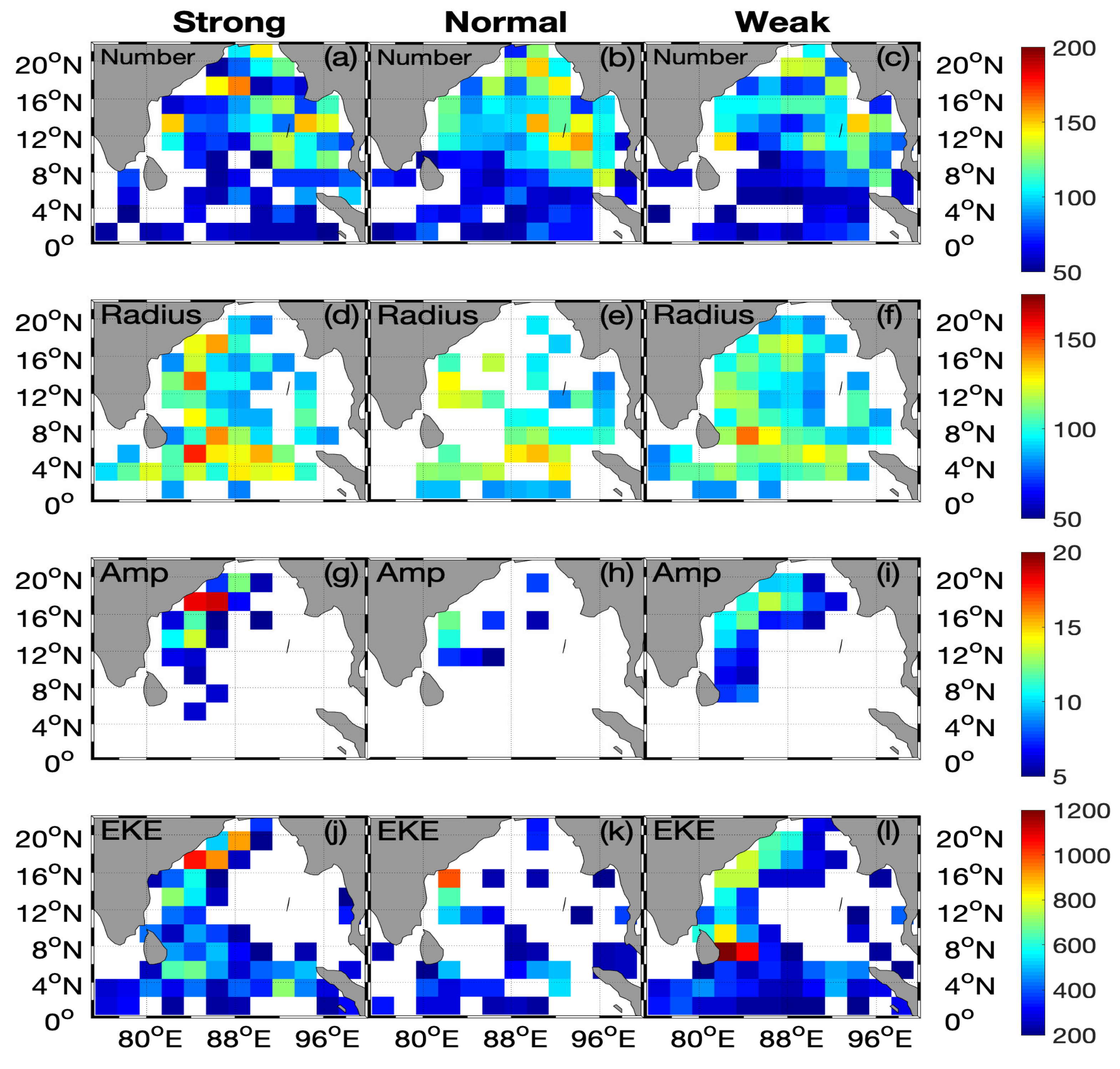
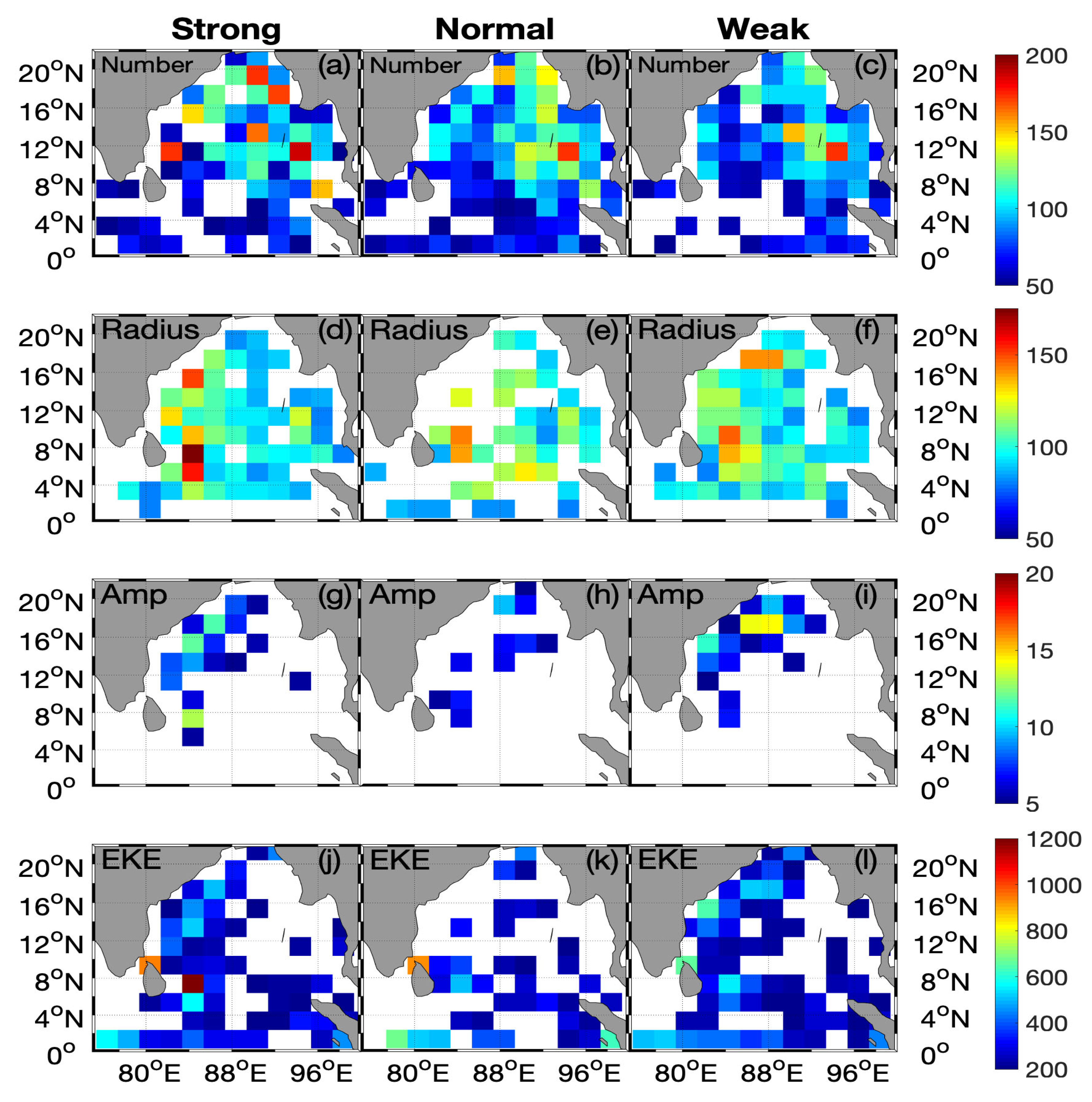
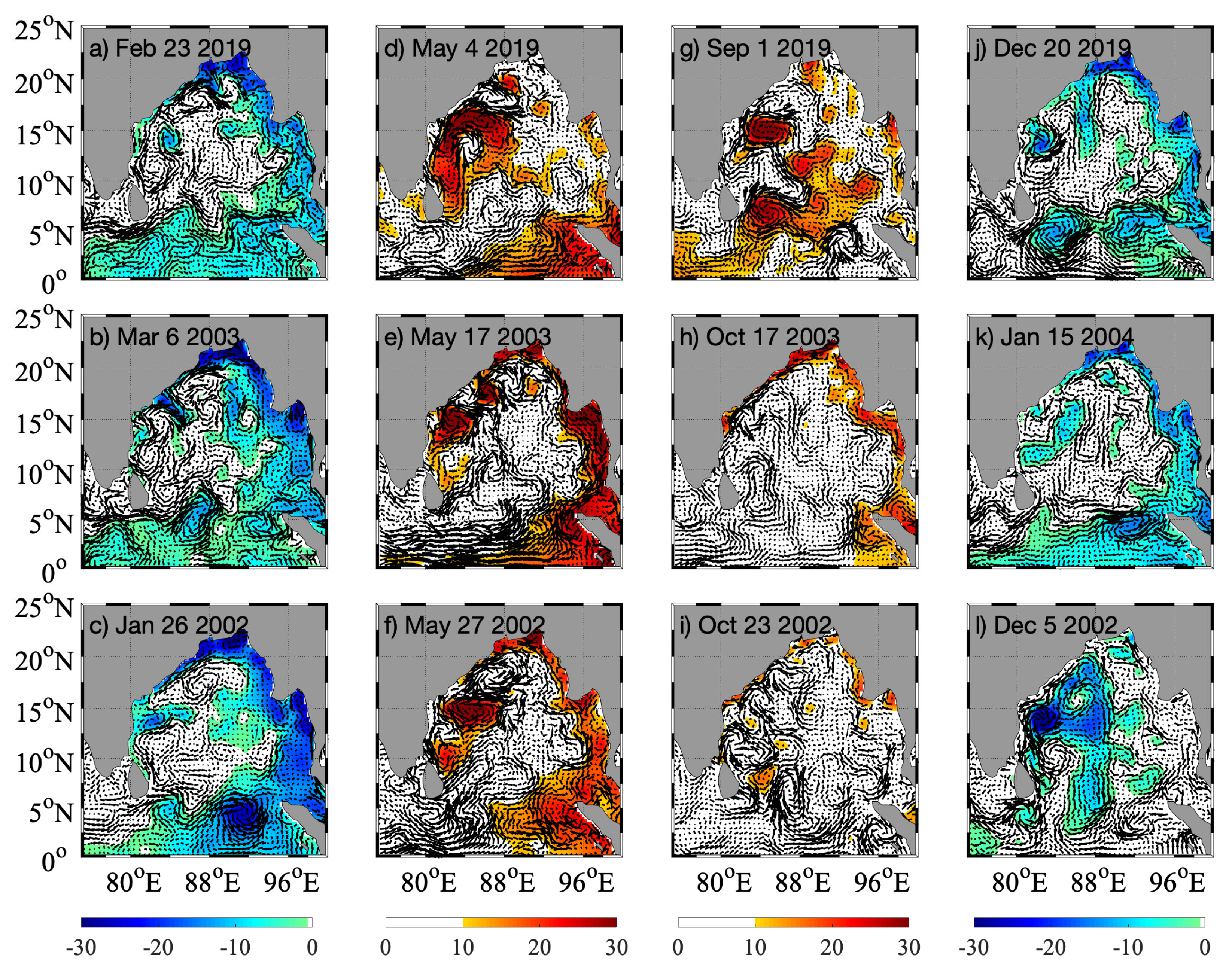
3.1. Spatial Eddy Characteristics in the Bay of Bengal

The spatial distribution of mean eddy properties throughout the BoB during strong, normal, and weak summer monsoon seasons is shown in Figure 1 and Figure 2. To emphasize regions of eddying that have the most direct impact on local air–sea interactions and present the most meaningful results, we have applied thresholds of 50 eddies (Figure 1a–c and Figure 2a–c), radii of 50 km (Figure 1d–f and Figure 2d–f), amplitudes of 5 cm (Figure 1g–i and Figure 2g–i), and eddy kinetic energy (EKE) of 200 cm2 s−2 (Figure 1j–l and Figure 2j–l). Pixels with values lower than these thresholds have been removed, and these regions appear white in these figures. Figure 1 represents cyclonic eddies (CEs), while Figure 2 represents anticyclonic eddies (AEs). The highest number of cyclonic eddies is along the northern and eastern coastlines of the BoB, with a more northern positioning as monsoon strength increases (Figure 1a–c). The latter could be due to coastal Kelvin waves in eastern Bay, as it is a source of upper ocean instability in this region [10,39]. There are more AEs than CEs during strong monsoon regimes, while there are more CEs than AEs during normal monsoon conditions. The regions of the largest cyclonic eddy radii vary greatly during monsoon regimes of different intensities. The largest cyclonic eddy radii, amplitudes, and EKEs for CEs were found during the strong monsoon regime (Figure 1d–f and 1g–i). The EKEs of CEs were strongest along the EICC, consistent with high-amplitude (>20 cm) eddying (Figure 1j–l).
For anticyclonic eddies (Figure 2), the spatial distribution of the number of eddies (Figure 2a–c) is similar to that of cyclonic eddies (Figure 1a–c), but with a local maximum of eddying in strong monsoon regimes along the east coast of India at 12°N consistent with the meandering of the EICC. The anticyclonic eddy adjacent to the Sri Lanka Dome region is visible in all years, although it is notably more robust during strong monsoon regimes (higher radius, amplitude, and EKE; Figure 2d–i). During weak monsoon regimes, there is anticyclonic eddying of a relatively moderate size class (~130 km radius in panel 2f compared with 20 km radius in panel 2d) in the northern Bay. High-amplitude anticyclonic eddies, like their cyclonic counterparts, are centralized about the EICC. The EKE of anticyclonic eddies clearly shows higher values in the EICC, equatorial Kelvin wave zone, and a local maximum east of Sri Lanka in a strong monsoon regime (Figure 2j–l).
Figure 3a–r shows the surface circulation as derived from the distributions of SLA for selected months—January, March, May, July, September, and November for the cases of strong monsoon (left column), normal monsoon (middle column), and weak monsoon (right column) years. During January, the peak of the winter monsoon season, one can see an anticyclonic circulation with higher SLA in the northwestern Bay (Figure 3a–c). This feature is present in all three monsoon regimes but has the highest SLA during strong conditions. A large cyclonic circulation cell also developed off the southeastern coast of India, which is absent in the years of strong and weak monsoons (Figure 3a–c). This particular cell was investigated using high-frequency radar by [68]. However, in all monsoon regimes, the westward flow is strong to the south of the Sri Lankan coast and is fed by the broad westward-flowing North Equatorial Current (NEC) during normal and weak monsoon regimes. During March, the arrival of the coastally trapped upwelling Kelvin wave on the east coast of India from the head of the Bay combines with the feeding of the NEC flow into the southeastern coast to constitute the poleward-flowing EICC. The EICC’s strength is high during the strong monsoon regime and weak during the weak monsoon regime due to the curtailed feeding of the NEC (Figure 3d–f). The western BoB is dominated by this dipolar pattern of high SLA to the west and low SLA to the east throughout March (Figure 3d–f). The high SLA on the western edge of the Bay intensifies to a complete, robust anticyclonic circulation that is most intense during the strong monsoon regime when it is bounded by a coherent cyclonic eddy centered at about 87°E and 18°N.
During May, the flow regime in the western Bay encapsulates alternating mesoscale anticyclonic and cyclonic eddies, with strong flows at their common boundaries in both the strong and weak monsoon regimes (Figure 3g–i). In contrast, a single large and narrow elongated anticyclonic eddy with swift flows develops in the northwestern Bay during the normal monsoon regime (Figure 3h). The onset of seasonal reversal of flow replacing the NEC is seen in the southern Bay, with the entry of eastward flow closer to the Sri Lankan coast during the strong monsoon regime (Figure 3g) and in the southeastern Bay during the weak monsoon regime (Figure 3i).
During July, one can see the entry of the strong Southwest Monsoon Current (SMC) closer to the Sri Lankan coast from the southwestern Bay to the central Bay. There is an anticyclonic eddy to its right and a cyclonic eddy to its left, just off Sri Lanka. At the same time, the May circulation in the western BoB is partly modified during the strong monsoon regime (Figure 3j). By contrast, during the normal monsoon regime, entry of the SMC into the central Bay is shifted eastward, and a cyclonic eddy is well defined offshore of Sri Lanka (Figure 3k); during the weak monsoon regime, the SMC is further shifted eastward with the consequent strengthening of cyclonic flow to its left in the central Bay and anticyclonic flow to its right in the southeastern Bay (Figure 3l). Among the monsoon regimes, the sea level reaches higher values in the Andaman Sea and along the northeastern coast of the Bay of Bengal during the weak monsoon regime, although there is more extreme alternation between positive and negative SLA during the strong monsoon consistent with an active eddy field. This surface circulation agrees well with observations reported by [5] for the normal monsoon of 1984.
By September, the SMC and its associated anticyclonic and cyclonic eddies that prevailed offshore of Sri Lanka during July have propagated westward. This propagation is in the form of a strong anticyclonic eddy and a weak cyclonic eddy that enter the southeastern Bay during the different monsoon regimes (Figure 3m–o). Alternating anticyclonic and cyclonic eddies occur in the western Bay during the strong monsoon regime, while a few eddies were noticed in the northern Bay during the weak monsoon regime. In the normal monsoon regime, cyclonic eddies dominate the western Bay, and anticyclonic eddies dominate the eastern Bay.
By November, during the strong monsoon regime, the circulation is chaotic with multiple mesoscale eddies, while during the normal and weak monsoon regimes, an equatorward flowing EICC associated with higher SLA is developed. The sea level is high and positive along the eastern rim of the BoB and Andaman Sea under the influence of downwelling Kelvin wave propagation from the equatorial region. The westward bending of the EICC is evident south of Sri Lanka during all monsoon regimes (Figure 3p–r).
Figure 4 presents the surface and vertical characteristics of the Sri Lanka Dome (SLD, cyclonic eddy) that developed off Sri Lanka in July during the different monsoon regimes based on NEMO model simulations [73]. The central axis of the SLD is located at 9° latitude during strong monsoon regimes and at 8°N and 7°N latitudes during normal and weak monsoon regimes, respectively. Vertical sections of density, salinity, temperature, and vertical velocity are presented along the zonal section (~9°N latitude) crossing the SLD during the strong monsoon regime (Figure 4a–c). Warm and high salinity waters occupy the center of the SLD, and as a consequence, SLA at the center of the SLD is weakly negative during the strong monsoon regime (Figure 4a–c). The center of the SLD is more intense, with the lowest negative SLA during the normal and weak monsoon regimes (Figure 4h,o), coinciding with intensified cyclonic currents in the SLD. In the normal regime, SLD encounters high (>34) salinity and cooler (~28 °C) surface waters (Figure 4i,j). In contrast, cooler and higher salinity surface waters appear in the SMC flow, while warmer (29.2–29.8 °C) and low (33.0–33.2) salinity surface waters occur on the western flank of the SLD during the weak monsoon regime (Figure 4o–q).
During the normal monsoon regime, the vertical extent of the SLD is limited to 200 m depth, whereas for the cases of strong and weak monsoon regimes, the cyclonic eddy reaches beyond 300 m depth, albeit with a weaker surface swirl (meridional component) velocity (0.2 ms−1). Swirl velocity refers to the tangential flow relative to the frame of reference. For a zonal cross-section, this is represented by meridional flow; for a meridional cross-section, this is represented by zonal flow. The positive swirl velocity (northward flow) and negative swirl velocity (southward flow) in the vertical describe the cyclonic eddy flows. During the normal and weak monsoon regimes, when the SLD is intensified, the surface swirl velocity reaches higher values (>0.6 ms−1) (Figure 4m,t). The vertical velocity is very weak in the upper 50 m and is strong (1 × 10⁻⁴ ms−1) in the thermocline region during the strong and normal monsoon regimes. This is juxtaposed with its state during the weak monsoon regime, where the vertical velocity is relatively high (0.5 × 10⁻⁴ ms−1) in the upper 50 m (Figure 4g,n,u).

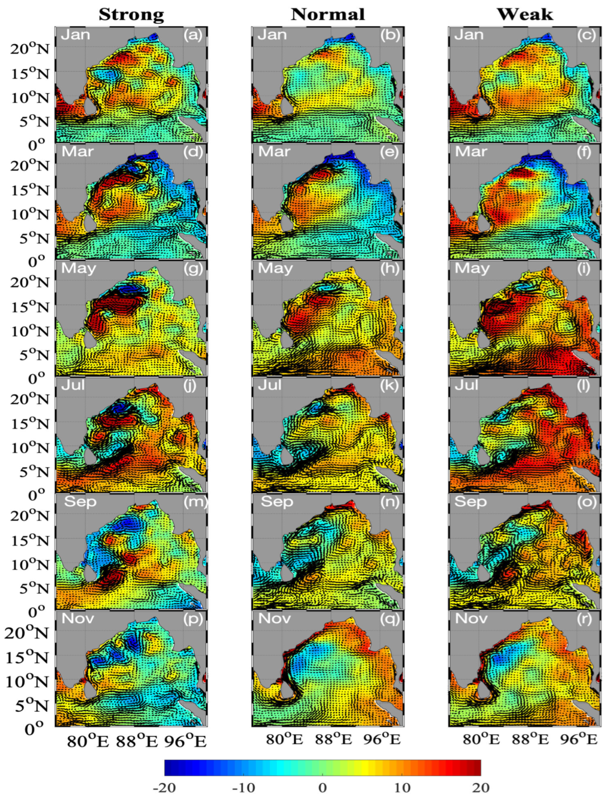
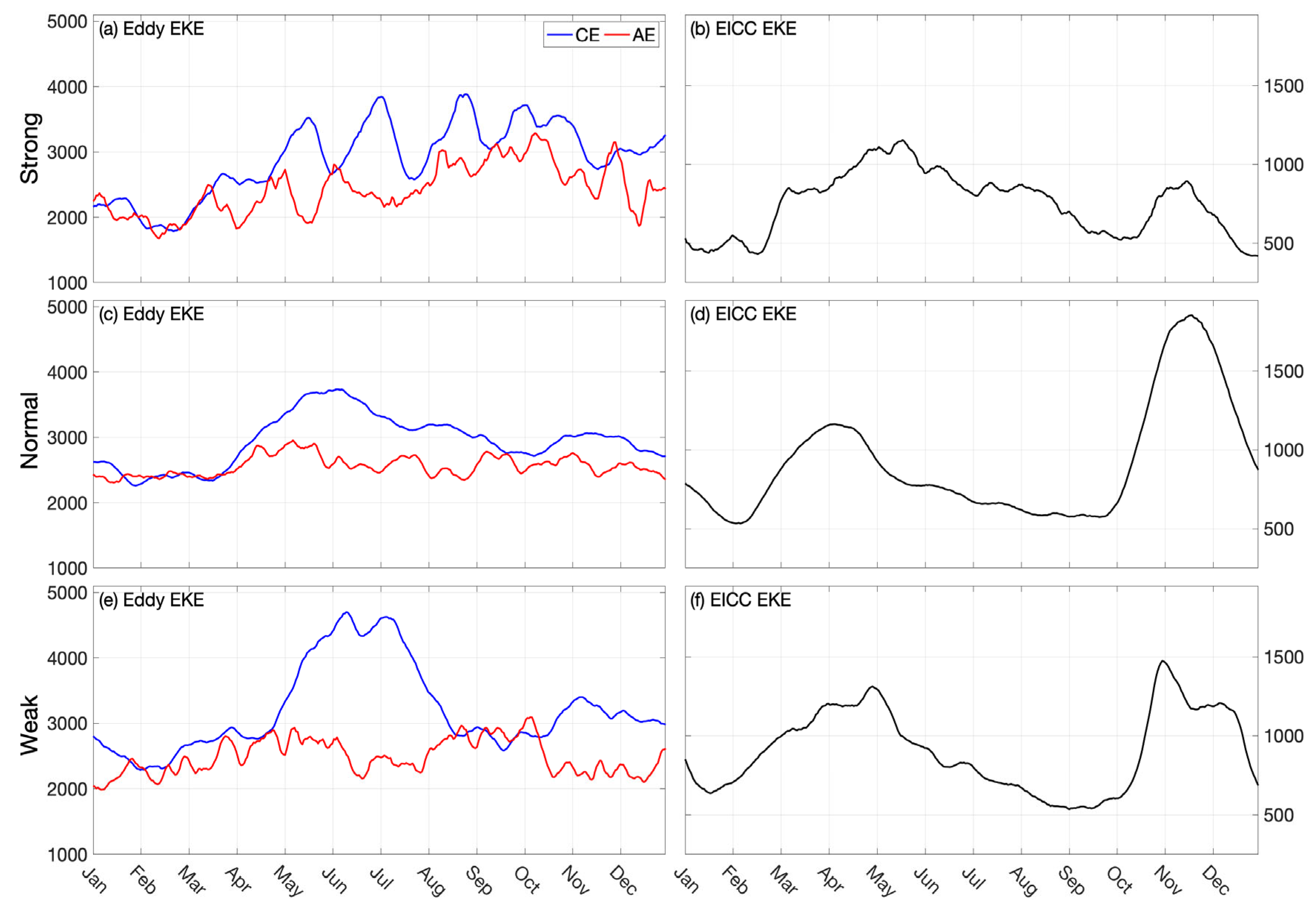
3.2. Temporal Eddy Characteristics in the Bay of Bengal

Figure 5a,c,e represent the seasonal variation of EKE for the cyclonic and anticyclonic eddies averaged over the region (75°E–100°E, 0°–24°N) for the strong, normal, and weak monsoon regimes. Figure 5b,d,f represents the EKE of the EICC regime over a width of 200 km from the east coast of India. Generally, the EKE of cyclonic eddies is larger than that of anticyclonic eddies, and the EKE peaks to a higher value (4000–5000 cm2 s−2) in May through July and drops to a lower value (1800–2000 cm2 s−2) in February during the different monsoon regimes (Figure 5a,c,e). The minimum EKE occurs in February during all three monsoon regimes. In the weak monsoon regime, the EKE of cyclonic eddies increases sharply in May and remains high until September, while the EKE of anticyclonic eddies remains relatively steady (Figure 5e). Corresponding to the poleward flowing EICC and equatorward flowing EICC, the EKE reaches maximum values in May and November–December during the different monsoon regimes (Figure 5b,d,f). During the strong monsoon regime, the EICC EKE reaches a high in May (1200 cm2 s−2; poleward EICC), and the equatorward EICC attains a secondary peak (800 cm2 s2) in mid-November (Figure 5b). The EICC EKE is high (1200 cm2 s−2) in April (poleward) and very high (1800 cm2 s−2) in November–December (equatorward) during the normal monsoon regime (Figure 5d). The EICC EKE reaches 1300 cm2 s−2 in May (poleward EICC) and 1500 cm2 s−2 in November (equatorward EICC) during the weak monsoon regime, with the lowest EKE (500 cm2 s−2) in September (Figure 5f).
A comparison of EKE in the western Bay and eastern Bay shows that the western Bay is dominated by larger and fewer eddies than its eastern counterparts. The eastern Bay is dominated by many small eddies, commonly generated by coastal Kelvin waves, which are in agreement with the findings of [20,21]. Weak monsoon conditions are the only scenarios that show strong CEs, with peaks in March, June, and July in the eastern BoB (Figure 6f). The western Bay is cyclonic eddy dominated during the first half of the strong monsoon year, and anticyclonic eddy dominated after July, indicating a direct seasonal response to basin-scale monsoon-directed flow (Figure 6a,c,e). In fact, the strong monsoon condition was the only one under which AEs dominated after July. The maximum CE EKE in the western Bay is similar between all years, with values of about 6000 cm2 s−2 (closer to 7000 cm2 s−2 in the strong monsoon conditions). The temporal period when AE EKEs exceed CE EKEs in the western Bay strongly varies from less than a month during normal conditions in early September to a three-month period in the strong monsoon from mid-July to mid-October (Figure 6a,c,e). In the eastern Bay (Figure 6b,d,f), the values of AE EKEs and CE EKEs are about the same, fluctuating around 2000 cm2 s−2. There is a period from March through July, when the eastern Bay’s EKE is dominated by CEs during weak and normal monsoon regimes (Figure 6d,f), but fluctuates between AE- and CE-dominant for strong monsoons (Figure 6b).

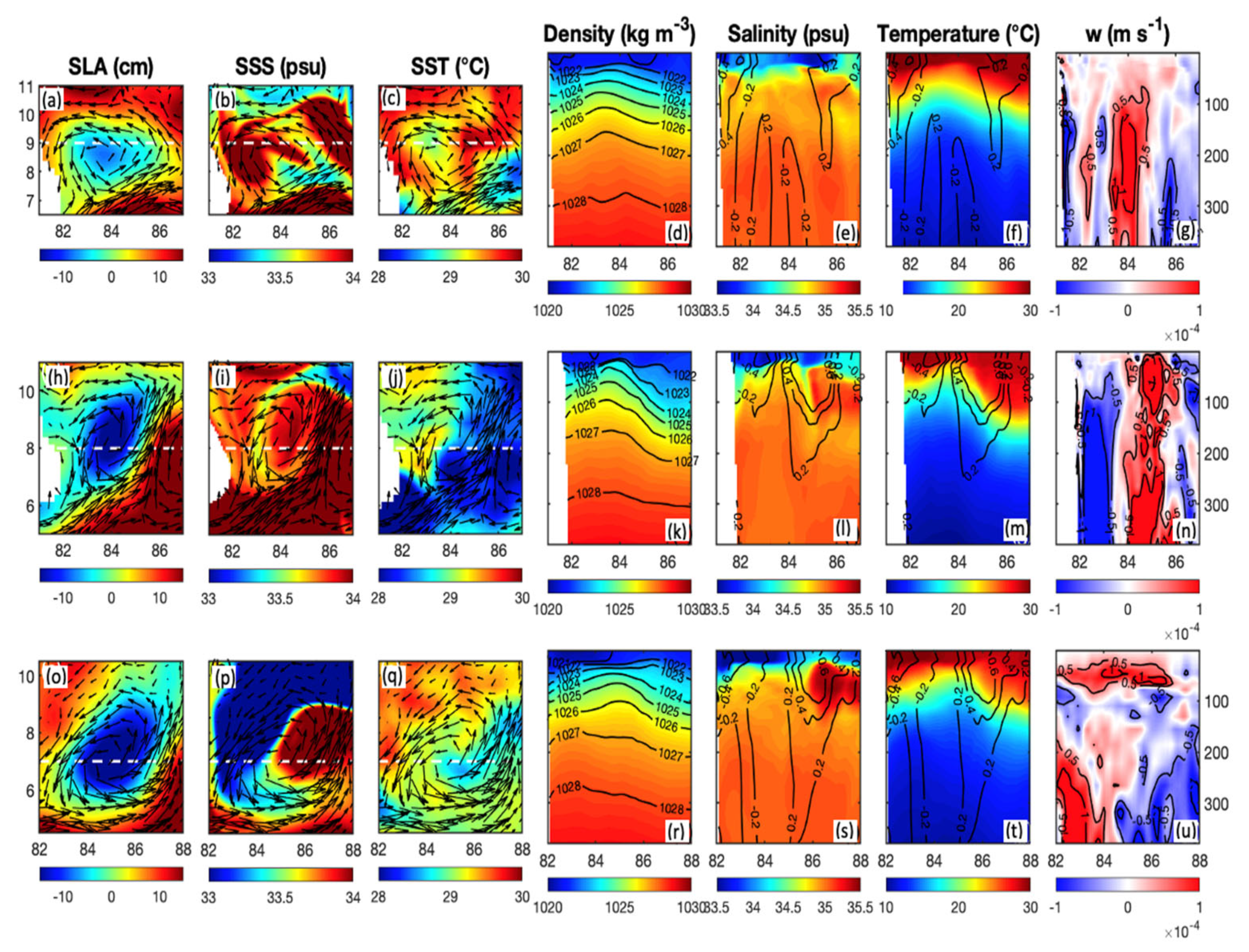
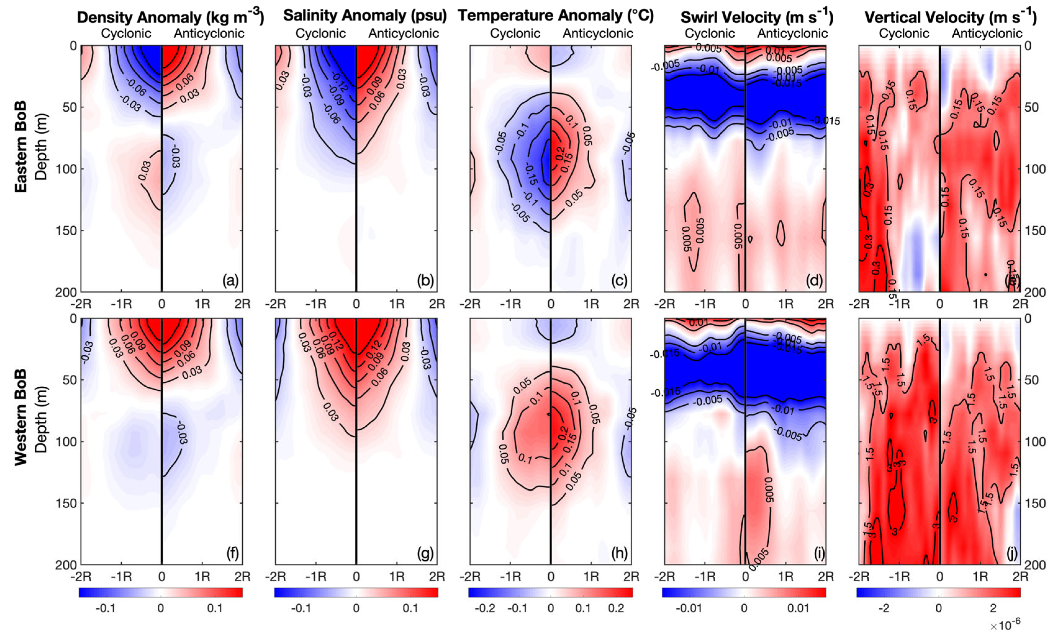
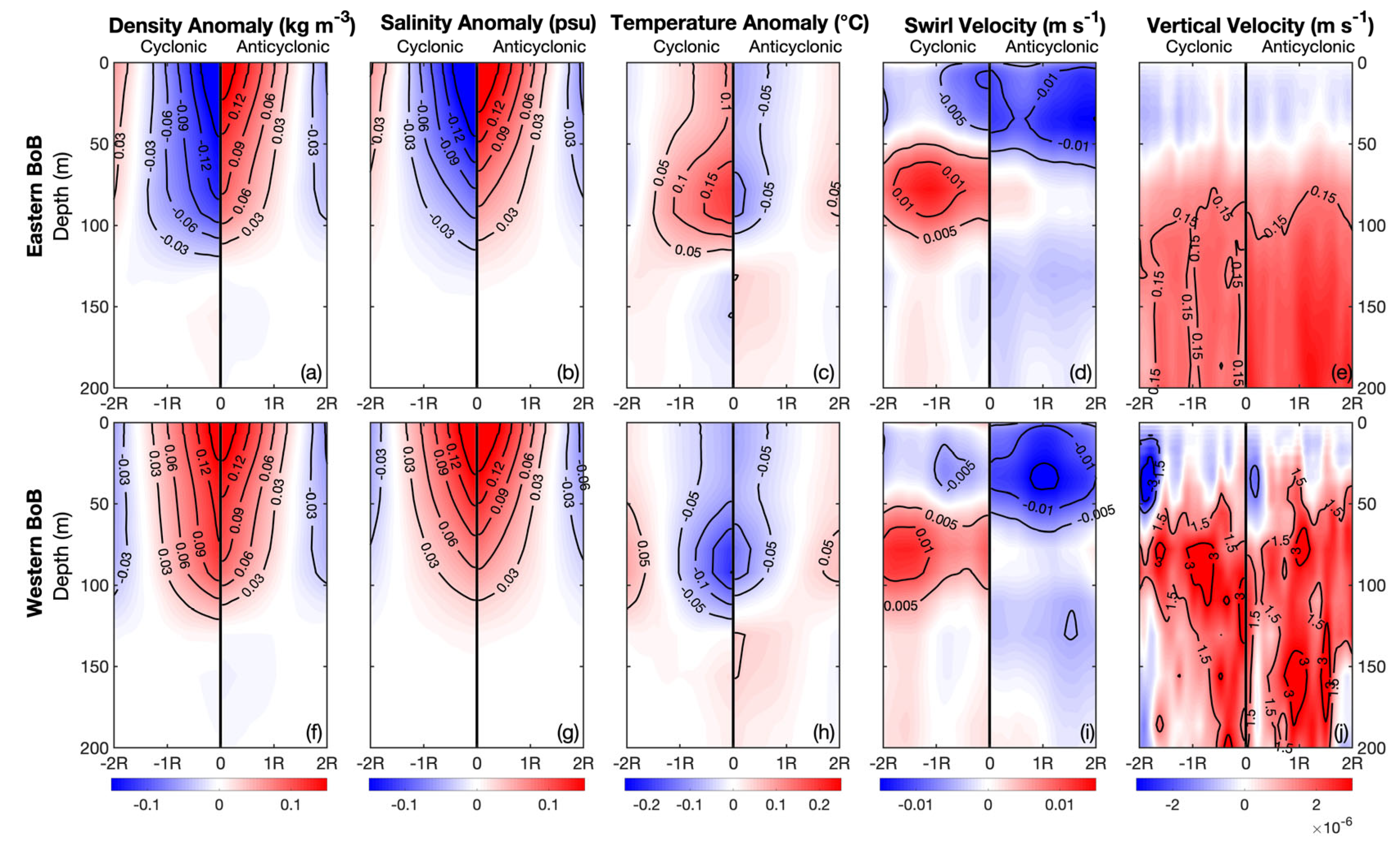
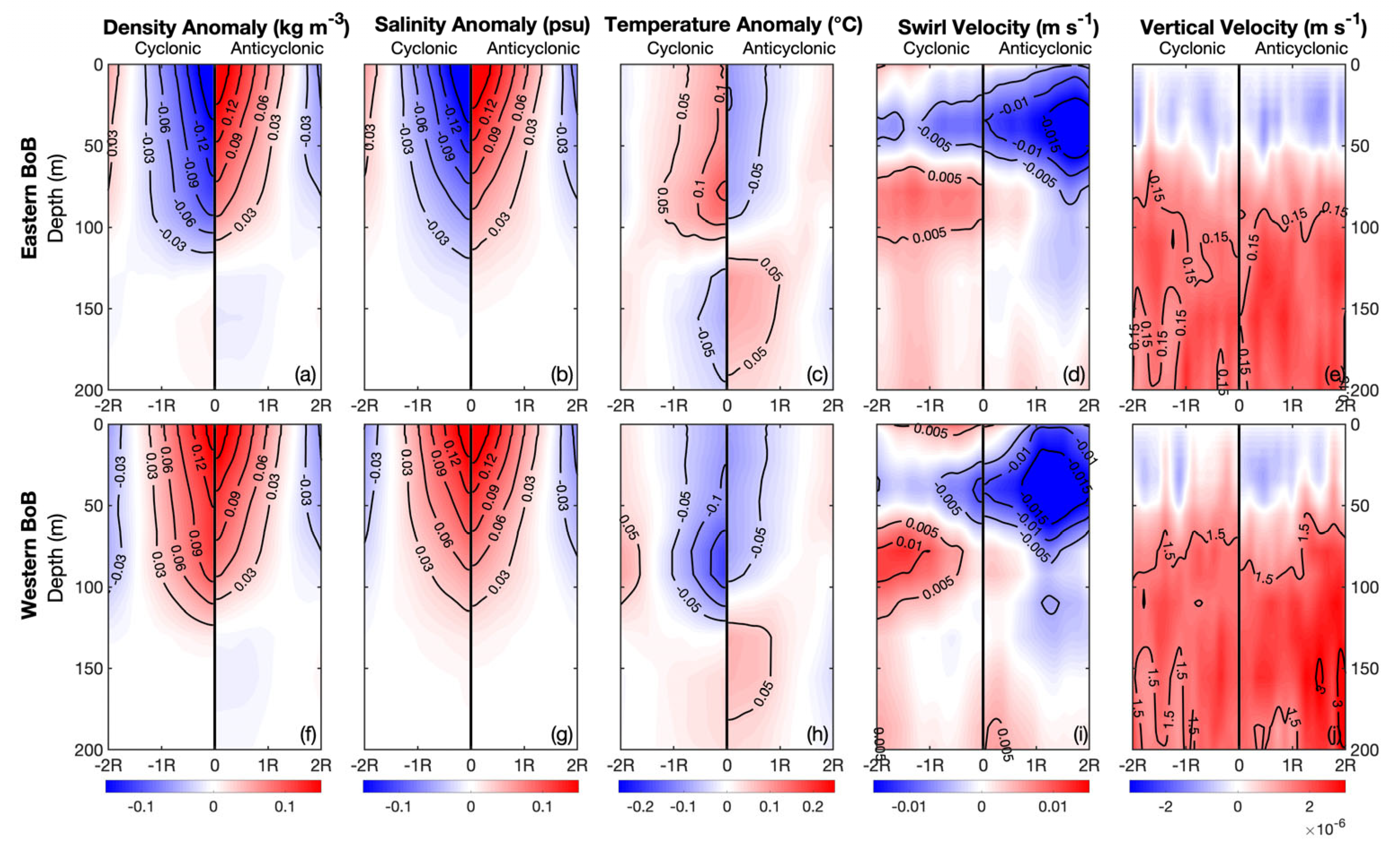
3.3. Eddy Characteristics as a Function of Depth

Vertical composites reveal the mean structure of eddies in the BoB and can provide insight into how they affect both local stratification and the water column as a whole. In the eastern BoB, density anomalies are dominated by salinity in the upper 50 m and by temperatures between 50 m and 150 m for strong monsoon seasons (Figure 7). The anomalies of density, salinity, and temperature are negative for cyclonic eddies and positive for anticyclonic eddies in the eastern BoB. In the western BoB for both the CEs and AEs, density anomalies at about the 100 m depth are influenced by the subsurface temperature anomaly, while those in the upper 50 m more closely mirror the salinity anomalies. Interestingly, the anomalies of density, salinity, and temperature are positive for both CEs and AEs. Fluctuations in the depth of the thermocline can be the source of such strong subsurface temperature anomalies. Composite swirl velocity anomalies (meridional component of velocity) show alternate flows in depth with a strong southerly flow below the salinity stratified surface layer. AEs have a deeper swirl velocity than CEs by about 25 m depth in the western Bay, while in the eastern Bay, both the CEs and AEs have similar swirl velocity structures. Vertical velocity anomalies are positive in both regions for both circulation types. The upwelling velocity is weaker in the CEs and AEs in the eastern Bay when compared to that in the western Bay for both CEs and AEs. This was the same result as that found in [20,33]. Similar subsurface patterns are seen in the normal monsoon season (Figure 8) and the weak monsoon season (Figure 9), although there appears to be shallowing in the vertical structures with increasing monsoon intensity. As monsoon intensity weakens, the eddy vertical structure increases. The temperature anomaly structure also deepens, but the swirl velocity anomaly becomes less extreme, so these eddies are deeper but weaker. In addition, in the weak monsoon year, we see some minor downwelling at the surface.

3.4. Coastal Kelvin Wave and Eddy Interactions

Figure 10 shows the variation of SLAs and the associated surface geostrophic currents during the propagation of the first upwelling Kelvin wave (Figure 10a–c), first downwelling Kelvin wave (Figure 10d–f), second downwelling Kelvin wave (Figure 10 g–i), and second upwelling Kelvin wave (Figure 10j–l) along the coasts of Sumatra and the Andaman Sea from the equatorial Indian Ocean. Since we are focusing on the different monsoon regimes, we will concentrate on the SLA distributions during the propagation of the first downwelling and second upwelling Kelvin waves during the strong monsoon regime (Figure 10d,j), the normal monsoon regime (Figure 10e,k), and the weak monsoon regime (Figure 10f,l). During the strong monsoon regime, large mesoscale AEs are generated in both the western Bay and east of Sri Lanka (Figure 10g), while smaller mesoscale AEs are generated in the central and northern Bay (Figure 10d,j). A large-scale CE or Sri Lanka Dome (SLD) is also generated off eastern Sri Lanka (Figure 10d,j). During the normal monsoon regime (2003), a cyclonic SLD is generated on the western flank of a strong SMC, while elongated AEs are generated on the right flank. Smaller mesoscale AEs and CEs are generated elsewhere in the BoB (Figure 10e,h,k). During the weaker monsoon regime (2002), the currents associated with the SMC, AEs, and SLD are strong (Figure 10c,f,i,l); mesoscale AEs are dominant elsewhere during the first downwelling Kelvin wave propagation (Figure 10f).
Hovmöller diagrams of SLA at the select latitudes (18°N, 15°N, 10°N and 5°N) during the different monsoon regimes as well as the SLA differences between strong monsoon and weaker monsoon regimes are presented in Figure 11. During the strong monsoon regime, one can see the propagation of AEs and CEs on the westward propagating Rossby wave radiated from the Myanmar coast (Figure 11a,e,i), with smaller (higher) SLAs during the strong (weaker) monsoon regime. This results in large negative SLAs (Figure 11m). Besides the westward propagation of upwelling and downwelling Rossby waves, SLAs in the northern Bay are also affected by strong (weaker) monsoon wind forcing, associated Ekman pumping, and surface convergences and divergences. During the weak monsoon regime (January–December 2002), westward propagating higher SLA, representing the downwelling Rossby wave, is evident at 18°N. It takes about 6 months (June to December) for this wave to travel from east to west at 18°N. The lower SLA on the east in March–April is associated with the generation of the weaker first upwelling Rossby wave, and the westward propagating higher SLA (May–October) represents the 2nd downwelling Rossby wave of the previous year (November–December 2013).
At 5°N, the westward propagation of Rossby waves is dominant. SLAs are large and positive during the monsoon seasons (May–September) of all regimes, resulting in weaker differences in SLA (Figure 10p). The 10°N latitudes extend into the Andaman Sea, and the variation of SLA at the eastern longitude (>95°E) represents its association with the coastal Kelvin wave and its westward radiation as a Rossby wave. During the weak monsoon regime, the first upwelling Kelvin wave (SLA, −10 cm) occurs from February–March, followed by downwelling Kelvin waves (SLA, +10 to +20 cm) from May to August and then from October to December (Figure 11k). During the strong and normal monsoon seasons (Figure 11c,g), only the downwelling Kelvin wave during June–September is apparent. SLA differences between the strong and weaker monsoon regimes are higher and positive at 15°N and weaker yet positive at 10°N (Figure 11n,o). The patterns of differences describe the propagation of eddies on the background Rossby waves (Figure 11p).

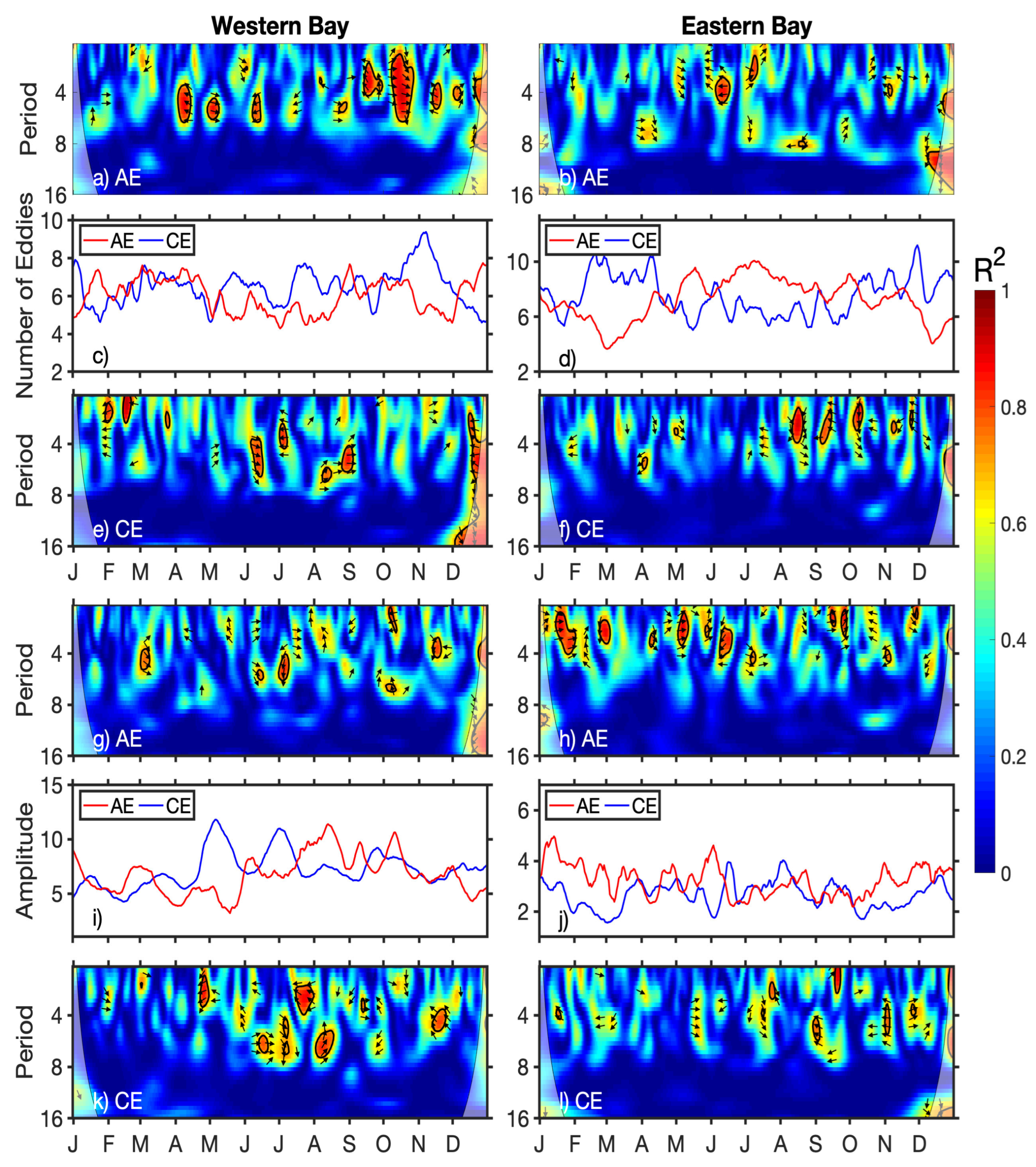
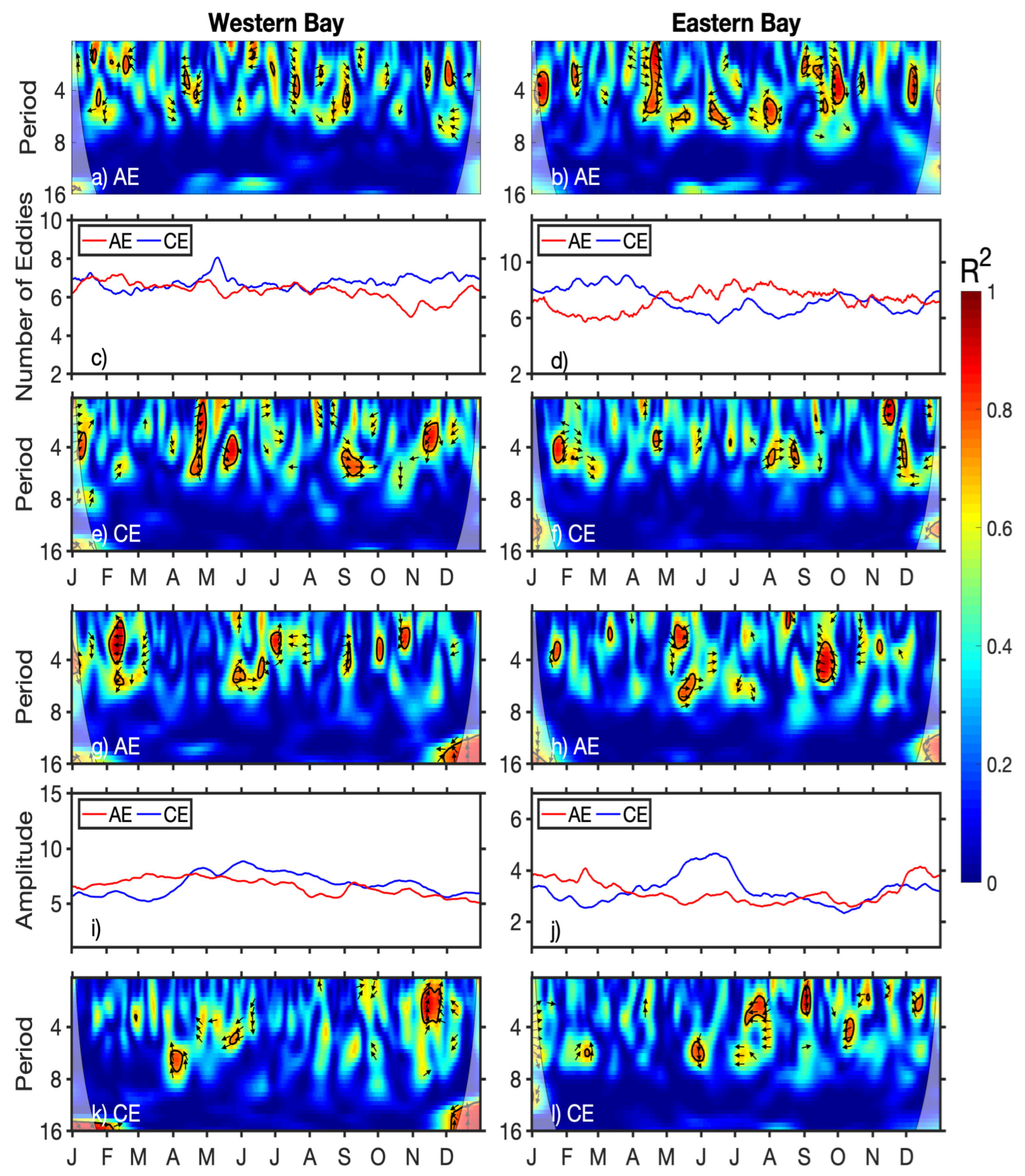
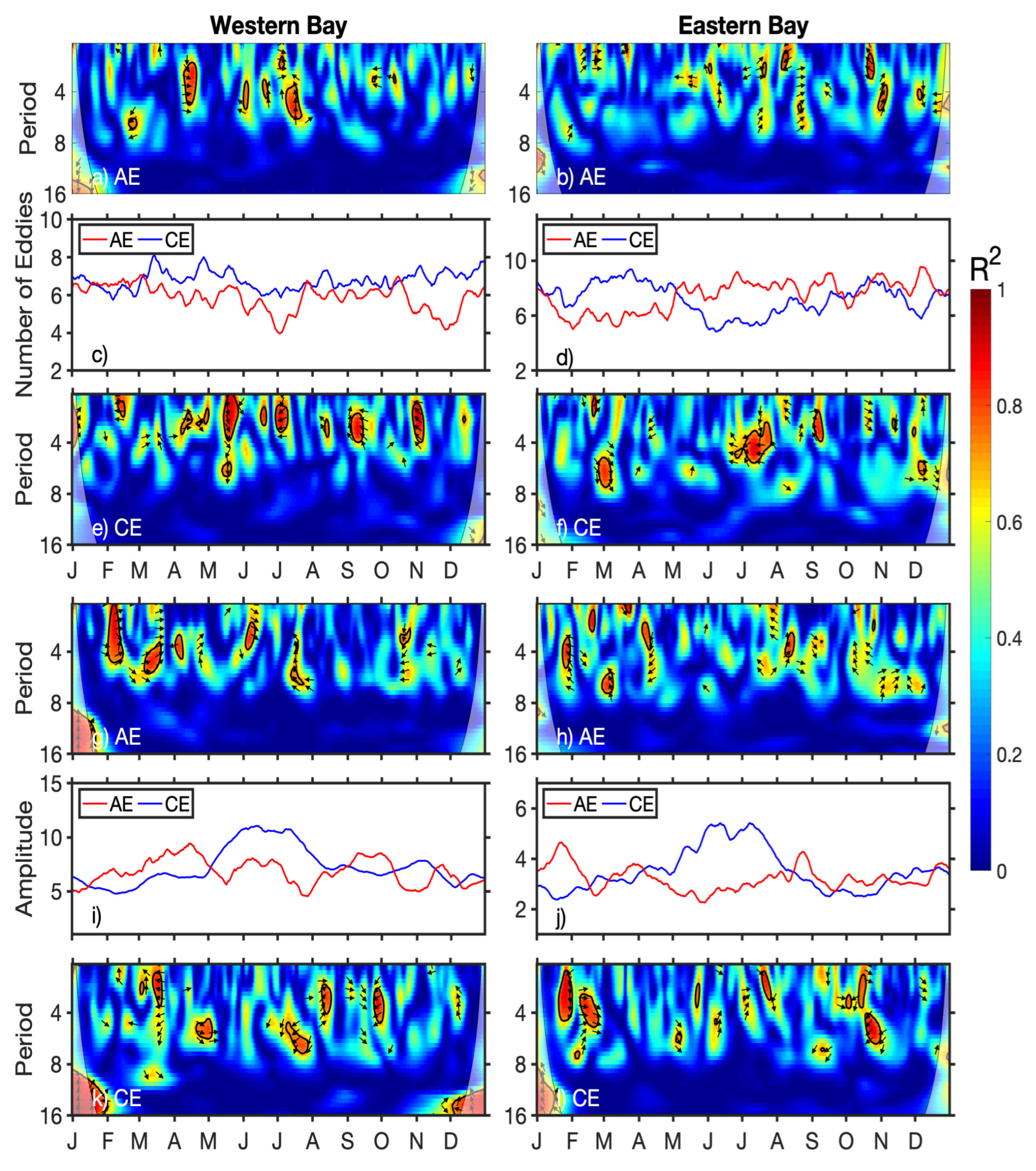
3.5. Wavelet Analysis

To provide statistical confirmation of the relationship between the eddy parameters observed and atmospheric precipitation and OHC, wavelet coherence analysis was conducted for all three monsoon regimes and is presented in Figure 12, Figure 13 and Figure 14 for the western and eastern Bay regions separately. It should be noted, however, that due to the comprehensive action of many factors that influence precipitation, including thermal, dynamic, water vapor and microphysical processes, this is an oversimplification. Future work is needed to isolate each individual forcing, which is outside the scope of this paper. There is higher wave coherence between the number of AEs and precipitation than the CEs during the strong monsoon regime, particularly in the western BoB during October and the post-monsoon period (Figure 12a–f). In the eastern BoB, the relationship between the number of AEs and precipitation was coherent during June–July. Similarly, the relationship between the number of CEs and precipitation was coherent during the intermonsoon periods. There was a more annually consistent relationship with minimal seasonal fluctuations during the normal monsoon regimes between the number of AEs and precipitation for both zonal halves of the BoB (Figure 13). The relationship between the number of CEs and precipitation was more coherent in the western BoB than in the eastern BoB and was strongest during the intermonsoon periods (Figure 13e). This was also true for high-amplitude CEs in the western Bay, but the relationship between high-amplitude CEs and precipitation in the eastern Bay peaked during the summer monsoon (Figure 13l). The relationship between the number of AEs and precipitation was again relatively strong throughout the year but was particularly coherent in March, August, and September (Figure 13b). The weak monsoon regime is the only one that shows a relatively similar wave coherence response between the eastern and western Bay (Figure 14). The relationship between the number of eddies and precipitation is slightly stronger for AEs, while the relationship between eddy amplitude and precipitation is slightly stronger for CEs throughout the Bay, with no notable seasonality other than the June–July peak (Figure 14f).
To better understand the relationship between 3–7 day synoptic oscillations in precipitation and ocean heat content (OHC) and mesoscale eddy activity, we compared the number of eddies of each circulation type and their mean amplitudes. This allowed us to see if there was a stronger connection between eddy robustness or the number of eddies with synoptic variability in each monsoon regime (Figure 15, Figure 16 and Figure 17). During strong monsoon conditions (Figure 15), the amplitudes of AEs and CEs are large in the western Bay compared to those in the eastern Bay. In the western Bay in August, high-amplitude synoptic oscillations in precipitation and OHC coincide with high-amplitude AEs. This is due to the increased capacity of larger-amplitude eddies to exchange heat with the atmospheric boundary layer and initiate deep convection [35].
During normal monsoon conditions (Figure 16), the highest-amplitude AEs do not coincide with 3–7-day synoptic oscillations in precipitation and OHC, which is different from the strong monsoon year (Figure 15). There are more years with normal monsoon conditions, so the individual eddy characteristics are averaged out, leaving only the overall seasonal behavior. The weakest connection between eddy amplitudes and 3–7 day synoptic oscillations seen during weak monsoon conditions is likely due to less extreme air–sea interactions derived from weaker wind forcing (Figure 17).

4. Discussion

Eddying is a critical component of upper-level advection and can modulate or intensify monsoon rainfall, particularly 3–7-day oscillations in the monsoon trough, which we directly observe in this work. High-amplitude BoB eddy events corresponded with 3–7-day rainfall oscillations, particularly during strong monsoon seasons, providing a direct link between the distribution of the SLA field and extreme flooding events. We find that large eddies of either circulation type provide the capacity to trigger synoptic oscillations due to the enhanced local heat exchanges during monsoonal air–sea interactions over the BoB.
The largest cyclonic eddy radii with weaker amplitudes were found in weak monsoon conditions, indicating a geometrically much “flatter” eddy structure. However, as monsoon intensity weakens, the vertical structure of these eddies deepens. The temperature anomaly structure also deepens, but swirl velocity becomes insignificant due to substantial compensation by vertical motion, so these eddies are deeper but weaker. In the western BoB, density anomalies at approximately 100 m depth are influenced by subsurface temperature anomalies, while those in the surface layer more closely mirror salinity anomalies. This is due to the unusually high river discharge at the sea surface and the associated salinity stratification in the Bay of Bengal. We found weaker Kelvin waves in weaker monsoon conditions, likely due to the weaker surface winds and diminished air–sea flux exchanges. In the case of the weaker monsoon, eddies have a deep vertical structure, indicating that vertical mixing is strong, with minimum lateral mixing (which is confirmed by the surface structures discussed above). In the cases of strong and normal monsoon regimes, both CEs and AEs are shallower, indicating the importance of lateral mixing over vertical mixing. Lower EKEs during strong monsoon regimes (compared to normal and weaker monsoon regimes) might also be due to stronger vertical mixing into the deeper ocean.

5. Conclusions

We conducted a multi-parameter analysis of the eddy field during the strong, normal, and weak monsoon regimes from 1993–2019 and found the highest number of eddies along the coastlines of the Bay, while the most robust and energetic eddies were located at the meanders of the EICC. This pattern was true for both circulation types (anticyclonic and cyclonic eddies). For the first time, we extend this analysis to include the subsurface eddy structure over the 27-year period of study, finding deeper eddies in weaker monsoon seasons.
We describe the flow in each monsoon regime, paying particular attention to the EICC and SLD. The western Bay is cyclonic eddy-dominated during the first half of the strong monsoon year and then anticyclonic eddy-dominated after June, also indicating a direct seasonal response to basin-scale monsoon-driven flow. Cyclonic eddy EKE was strongest along the EICC region and 4°N, indicating the influence of energetic equatorial Kelvin waves and the westward propagating Rossby waves, respectively. The EKE of anticyclonic eddies clearly shows higher values in the EICC, equatorial Kelvin waves, and a local maximum off the Sri Lanka coast that is highest during a strong monsoon regime. In the normal monsoon regime, SLD contains high (>34) salinity and cooler (~28 °C) surface waters, under the influence of cyclonic divergent flows of this SLD. In contrast, cooler, and high salinity surface waters of the eastern Arabian Sea origin appear in the SMC flow on the eastern flank of the SLD. Interestingly, warmer (29.2–29.8 °C) and low (33.0–33.2) salinity surface waters occur in the southwestern Bay on the western flank of the SLD during the weak monsoon regime. During the normal monsoon regime, the vertical extent of the SLD (cyclonic eddy) is limited to 200 m depth, whereas for the cases of strong and weak monsoon regimes, the SLD reaches beyond 300 m depth but with a weaker surface swirl velocity (0.2 ms−1). Weak monsoon conditions are the only scenario with strong CEs in the eastern BoB.
Through the Hovmöller diagrams of SLA at 10° latitude and 5°N latitude, it can be seen that the first upwelling coastally trapped Kelvin waves appear during February 2014, while the first downwelling Kelvin wave appears from May to August. The second downwelling Kelvin wave appears in November–December. However, only downwelling Kelvin waves are apparent during June–September during strong and normal monsoon regimes. These variations in the propagation of coastal Kelvin waves during the monsoon regimes affected the eddy formations in the western Bay, as well as in the EICC.
Relationships between the 3–7-day synoptic oscillations in precipitation and OHC and the number of mesoscale eddies in each circulation type are examined for three monsoon regimes. In western Bay, high-amplitude synoptic oscillations align with high-amplitude AEs rather than the number of eddies. We find that large eddies of either circulation type provide the capacity to trigger synoptic oscillations, more clearly the AEs, due to the enhanced local heat exchanges during monsoonal air–sea interactions. The eddy amplitudes and 3–7-day synoptic oscillations are weakly connected during weak monsoon conditions. This is not unsurprising because weaker winds are associated with a weaker summer monsoon. Wavelet coherence analysis conducted for all three monsoon regimes (strong, normal, and weak) reveals stronger coherence between eddy amplitude and atmospheric precipitation and ocean heat content than the number of eddies.

Author Contributions

Conceptualization, B.S.; methodology, C.B.T. and B.S.; software, C.B.T.; validation, C.B.T. and B.S.; formal analysis, C.B.T. and B.S.; investigation, C.B.T. and B.S.; resources, B.S.; data curation, B.S.; writing—original draft preparation, C.B.T.; writing—review and editing, C.B.T. and B.S.; visualization, B.S.; supervision, B.S.; project administration, B.S.; funding acquisition, B.S. All authors have read and agreed to the published version of the manuscript.

Funding

This research is supported through the United States Office of Naval Research Award #N00014-17-1-2468 awarded to B.S. This has NRL contribution number JA-7320-21-5330. Approved for public release, distribution is unlimited.

Data Availability Statement

SLA data used in this research is courtesy of the Copernicus Marine Environmental Monitoring Service (CMEMS; https://data.marine.copernicus.eu/product/SEALEVEL_GLO_PHY_L4_MY_008_047/description accessed on 13 January 2023). CMEMS also provides the GLORYS12 model simulations used in this research (ftp://my.cmems-du.eu/Core/GLOBAL_REANALYSIS_PHY_001_030/global-reanalysis-phy-001-030-dail accessed on 13 January 2023). Daily precipitation is obtained from the European Centre for Medium-Range Weather Forecasts (ECMWF) ERA-Interim global atmospheric reanalysis (http://apps.ecmwf.int/datasets/data/interim-full-daily/levtype5sfc/accessed on 13 January 2023). SST data is obtained from NOAA’s National Climatic Data Center (NCDC) Optimally Interpolated SST. SMAP SSS is provided by NASA-JPL (smap.jpl.nasa.gov accessed on 13 January 2023).

Conflicts of Interest

The authors declare no conflict of interest. The funders had no role in the design of the study, in the collection, analyses, or interpretation of data, in the writing of the manuscript, or in the decision to publish the results.

References

  1. Shankar, D.; Vinayachandran, P.; Unnikrishnan, A. The monsoon currents in the north Indian Ocean. Prog. Oceanogr. 2002, 52, 63–120. [Google Scholar] [CrossRef]
  2. Cheng, X.; Xie, S.-P.; McCreary, J.P.; Qi, Y.; Du, Y. Intraseasonal variability of sea surface height in the Bay of Bengal. J. Geophys. Res. Oceans 2013, 118, 816–830. [Google Scholar] [CrossRef] [Green Version]
  3. Chen, G.; Li, Y.; Xie, Q.; Wang, D. Origins of Eddy Kinetic Energy in the Bay of Bengal. J. Geophys. Res. Oceans 2018, 123, 2097–2115. [Google Scholar] [CrossRef]
  4. Kurien, P.; Ikeda, M.; Valsala, V.K. Mesoscale variability along the east coast of India in spring as revealed from satellite data and OGCM simulations. J. Oceanogr. 2010, 66, 273–289. [Google Scholar] [CrossRef]
  5. Murty, V.S.N.; Sarma, Y.V.B.; Rao, D.P.; Murty, C.S. Water characteristics, mixing and circulation in the Bay of Bengal during southwest monsoon. J. Mar. Res. 1992, 50, 207–228. [Google Scholar] [CrossRef]
  6. Sreenivas, P.; Gnanaseelan, C.; Prasad, K. Influence of El Niño and Indian Ocean Dipole on sea level variability in the Bay of Bengal. Glob. Planet. Chang. 2012, 80, 215–225. [Google Scholar] [CrossRef]
  7. Rao, R.; Kumar, M.G.; Ravichandran, M.; Rao, A.; Gopalakrishna, V.; Thadathil, P. Interannual variability of Kelvin wave propagation in the wave guides of the equatorial Indian Ocean, the coastal Bay of Bengal and the southeastern Arabian Sea during 1993–2006. Deep. Sea Res. Part I Oceanogr. Res. Pap. 2010, 57, 1–13. [Google Scholar] [CrossRef]
  8. Nienhaus, M.J.; Subrahmanyam, B.; Murty, V.S.N. Altimetric Observations and Model Simulations of Coastal Kelvin Waves in the Bay of Bengal. Mar. Geodesy 2012, 35, 190–216. [Google Scholar] [CrossRef]
  9. Mandal, S.; Sil, S.; Gangopadhyay, A.; Jena, B.K.; Venkatesan, R.; Gawarkiewicz, G. Seasonal and Tidal Variability of Surface Currents in the Western Andaman Sea Using HF Radars and Buoy Observations During 2016–2017. IEEE Trans. Geosci. Remote. Sens. 2020, 59, 7235–7244. [Google Scholar] [CrossRef]
  10. Greaser, S.R.; Subrahmanyam, B.; Trott, C.B.; Roman-Stork, H.L. Interactions Between Mesoscale Eddies and Synoptic Oscillations in the Bay of Bengal During the Strong Monsoon of 2019. J. Geophys. Res. Ocean. 2020, 125, e2020JC016772. [Google Scholar] [CrossRef]
  11. Saji, N.H.; Goswami, B.N.; Vinayachandran, P.N.; Yamagata, T. A dipole mode in the tropical Indian Ocean. Nature 1999, 401, 360–363. [Google Scholar] [CrossRef] [PubMed]
  12. Ashok, K.; Chan, W.; Motoi, T.; Yamagata, T. Decadal variability of the Indian Ocean dipole. Geophys. Res. Lett. 2004, 31, 1–4. [Google Scholar] [CrossRef] [Green Version]
  13. Gadgil, S.; Asha, G. Intraseasonal Variation of the Summer Monsoon. J. Meteorol. Soc. Jpn. Ser. II 1992, 70, 517–527. [Google Scholar] [CrossRef] [Green Version]
  14. Gadgil, S.; Joseph, P.V. On breaks of the Indian monsoon. J. Earth Syst. Sci. 2003, 112, 529–558. [Google Scholar] [CrossRef] [Green Version]
  15. Goswami, B.N.; Ajayamohan, R.S.; Xavier, P.K.; Sengupta, D. Clustering of synoptic activity by Indian summer monsoon intraseasonal oscillations. Geophys. Res. Lett. 2003, 30, 1–4. [Google Scholar] [CrossRef] [Green Version]
  16. Murakami, M. Analysis of Summer Monsoon Fluctuations over India. J. Meteorol. Soc. Jpn. Ser. II 1976, 54, 15–31. [Google Scholar] [CrossRef] [Green Version]
  17. Subrahmanyam, B.; Roman-Stork, H.L.; Murty, V.S.N. Response of the Bay of Bengal to 3-7-Day Synoptic Oscillations During the Southwest Monsoon of 2019. J. Geophys. Res. Oceans 2020, 125, e2020JC016200. [Google Scholar] [CrossRef]
  18. Chen, G.; Wang, D.; Hou, Y. The features and interannual variability mechanism of mesoscale eddies in the Bay of Bengal. Cont. Shelf Res. 2012, 47, 178–185. [Google Scholar] [CrossRef]
  19. Cui, W.; Yang, J.; Ma, Y. A statistical analysis of mesoscale eddies in the Bay of Bengal from 22–year altimetry data. Acta Oceanol. Sin. 2016, 35, 16–27. [Google Scholar] [CrossRef]
  20. Dandapat, S.; Chakraborty, A. Mesoscale eddies in the Western Bay of Bengal as observed from Satellite Altimetry in 1993–2014: Statistical characteristics, variability and three-dimensional properties. IEEE J. Sel. Top. Appl. Earth Obs. Remote Sens. 2016, 9, 5044–5054. [Google Scholar] [CrossRef]
  21. Roman-Stork, H.L.; Subrahmanyam, B.; Trott, C.B. Mesoscale eddy variability and its linkage to deep convection over the Bay of Bengal using satellite altimetric observations. Adv. Space Res. 2019, 68, 378–400. [Google Scholar] [CrossRef]
  22. Patnaik, K.V.K.R.K.; Maneesha, K.; Sadhuram, Y.; Prasad, K.V.S.R.; Murty, T.V.R.; Rao, V.B. East India Coastal Current induced eddies and their interaction with tropical storms over Bay of Bengal. J. Oper. Oceanogr. 2014, 7, 58–68. [Google Scholar] [CrossRef] [Green Version]
  23. Gulakaram, V.S.; Vissa, N.K.; Bhaskaran, P.K. Role of mesoscale eddies on atmospheric convection during summer monsoon season over the Bay of Bengal: A case study. J. Ocean Eng. Sci. 2018, 3, 343–354. [Google Scholar] [CrossRef]
  24. Schott, F.A.; McCreary, J.P. The monsoon circulation of the Indian Ocean. Prog. Oceanogr. 2001, 51, 1–123. [Google Scholar] [CrossRef]
  25. Trott, C.B.; Subrahmanyam, B.; Murty, V. Variability of the Somali Current and eddies during the southwest monsoon regimes. Dyn. Atmos. Oceans 2017, 79, 43–55. [Google Scholar] [CrossRef]
  26. Mawren, D.; Reason, C.J.C. Variability of upper-ocean characteristics and tropical cyclones in the South West Indian Ocean. J. Geophys. Res. Oceans 2017, 122, 2012–2028. [Google Scholar] [CrossRef]
  27. Jangir, B.; Swain, D.; Ghose, S. Influence of eddies and tropical cyclone heat potential on intensity changes of tropical cyclones in the North Indian Ocean. Adv. Space Res. 2020, 68, 773–786. [Google Scholar] [CrossRef]
  28. Huang, M.; Liang, X.; Zhu, Y.; Liu, Y.; Weisberg, R.H. Eddies Connect the Tropical Atlantic Ocean and the Gulf of Mexico. Geophys. Res. Lett. 2021, 48, e2020GL091277. [Google Scholar] [CrossRef]
  29. Capet, A.; Taburet, G.; Mason, E.; Pujol, M.I.; Grégoire, M.; Rio, M.-H. Using Argo Floats to Characterize Altimetry Products: A Study of Eddy-Induced Subsurface Oxygen Anomalies in the Black Sea. Front. Mar. Sci. 2022, 9, 842. [Google Scholar] [CrossRef]
  30. Mason, E.; Ruiz, S.; Bourdalle-Badie, R.; Reffray, G.; García-Sotillo, M.; Pascual, A. New insight into 3-D mesoscale eddy properties from CMEMS operational models in the western Mediterranean. Ocean Sci. 2019, 15, 1111–1131. [Google Scholar] [CrossRef] [Green Version]
  31. Sanikommu, S.; Toye, H.; Zhan, P.; Langodan, S.; Krokos, G.; Knio, O.; Hoteit, I. Impact of Atmospheric and Model Physics Perturbations On a High-Resolution Ensemble Data Assimilation System of the Red Sea. J. Geophys. Res. Oceans 2020, 125, e2019JC015611. [Google Scholar] [CrossRef]
  32. Rocha, C.B.; Simoes-Sousa, I.T. Compact Mesoscale Eddies in the South Brazil Bight. Remote Sens. 2022, 14, 5781. [Google Scholar] [CrossRef]
  33. Vu, B.L.; Stegner, A.; Charles, E.; Faugere, Y. (2019, January). An OSSE to quantify the reliability and the accuracy of au-tomatic eddy detection performed on gridded altimetric product. In Proceedings of the 21st EGU General Assembly, EGU2019, Vienna, Austria, 7–12 April 2019. In Geophysical Research Abstracts; EGU: Gottingen, Germany, 2019; Volume 21. [Google Scholar]
  34. Barboni, A.; Lazar, A.; Stegner, A.; Moschos, E. Lagrangian eddy tracking reveals the Eratosthenes anticyclonic attractor in the eastern Levantine Basin. Ocean Sci. 2021, 17, 1231–1250. [Google Scholar] [CrossRef]
  35. Stegner, A.; Le Vu, B.; Dumas, F.; Ghannami, M.A.; Nicolle, A.; Durand, C.; Faugere, Y. Cyclone-Anticyclone Asymmetry of Eddy Detection on Gridded Altimetry Product in the Mediterranean Sea. J. Geophys. Res. Oceans 2021, 126, e2021JC017475. [Google Scholar] [CrossRef]
  36. Zhu, Y.; Liang, X. Characteristics of Eulerian mesoscale eddies in the Gulf of Mexico. Front. Mar. Sci. 2022, 9, 2655. [Google Scholar] [CrossRef]
  37. Brokaw, R.J.; Subrahmanyam, B.; Trott, C.B.; Chaigneau, A. Eddy Surface Characteristics and Vertical Structure in the Gulf of Mexico from Satellite Observations and Model Simulations. J. Geophys. Res. Oceans 2020, 125, e2019JC015538. [Google Scholar] [CrossRef]
  38. Todd, R.E. Equatorial Circulation in the Western Indian Ocean During Onset of the 2018 Summer Monsoon and Links to the Bay of Bengal. Geophys. Res. Lett. 2020, 47, e2020GL087215. [Google Scholar] [CrossRef]
  39. Shoup, C.G.; Roman-Stork, H.L.; Subrahmanyam, B. Analysis of Coupled Oceanic and Atmospheric Preconditioning for Primary Madden-Julian Oscillation Events Across ENSO Phases. J. Geophys. Res. Oceans 2020, 125, e2020JC016358. [Google Scholar] [CrossRef]
  40. Feng, J.; Qiu, Y.; Dong, C.; Ni, X.; Lin, W.; Teng, H.; Pan, A. Interannual Variabilities of the Southern Bay of Bengal Cold Pool Associated with the El Niño–Southern Oscillation. Remote Sens. 2022, 14, 6169. [Google Scholar] [CrossRef]
  41. Ayouche, A.; De Marez, C.; Morvan, M.; L’Hegaret, P.; Carton, X.; Le Vu, B.; Stegner, A. Structure and Dynamics of the Ras al Hadd Oceanic Dipole in the Arabian Sea. Oceans 2021, 2, 105–125. [Google Scholar] [CrossRef]
  42. Roman-Stork, H.L.; Subrahmanyam, B.; Murty, V.S.N. The Role of Salinity in the Southeastern Arabian Sea in Determining Monsoon Onset and Strength. J. Geophys. Res. Oceans 2020, 125, e2019JC015592. [Google Scholar] [CrossRef]
  43. Le Traon, P.Y.; Nadal, F.; Ducet, N. An Improved Mapping Method of Multisatellite Altimeter Data. J. Atmos. Ocean. Technol. 1998, 15, 522–534. [Google Scholar] [CrossRef]
  44. Ducet, N.; Le Traon, P.-Y.; Reverdin, G. Global high-resolution mapping of ocean circulation from TOPEX/Poseidon and ERS-1 and -2. J. Geophys. Res. Oceans 2000, 105, 19477–19498. [Google Scholar] [CrossRef]
  45. Verezemskaya, P.; Barnier, B.; Gulev, S.K.; Gladyshev, S.; Molines, J.; Gladyshev, V.; Lellouche, J.; Gavrikov, A. Assessing Eddying (1/12°) Ocean Reanalysis GLORYS12 Using the 14-yr Instrumental Record From 59.5° N Section in the Atlantic. J. Geophys. Res. Oceans 2021, 126, e2020JC016317. [Google Scholar] [CrossRef]
  46. Berrisford, P.; Kållberg, P.; Kobayashi, S.; Dee, D.; Uppala, S.; Simmons, A.J.; Poli, P.; Sato, H. Atmospheric conservation properties in ERA-Interim. Q. J. R. Meteorol. Soc. 2011, 137, 1381–1399. [Google Scholar] [CrossRef]
  47. Reynolds, R.W.; Smith, T.M.; Liu, C.; Chelton, D.B.; Casey, K.S.; Schlax, M.G. Daily High-Resolution-Blended Analyses for Sea Surface Temperature. J. Clim. 2007, 20, 5473–5496. [Google Scholar] [CrossRef]
  48. Murty, V.S.N.; Subrahmanyam, B.; Tilvi, V.; O’Brien, J.J. A new technique for the estimation of sea surface salinity in the tropical Indian Ocean from OLR. J. Geophys. Res. Atmos. 2004, 109, 1–26. [Google Scholar] [CrossRef] [Green Version]
  49. Girishkumar, M.S.; Joseph, J.; Thangaprakash, V.P.; Pottapinjara, V.; McPhaden, M.J. Mixed Layer Temperature Budget for the Northward Propagating Summer Monsoon Intraseasonal Oscillation (MISO) in the Central Bay of Bengal. J. Geophys. Res. Oceans 2017, 122, 8841–8854. [Google Scholar] [CrossRef]
  50. Roman-Stork, H.L.; Subrahmanyam, B.; Murty, V. Quasi-biweekly oscillations in the Bay of Bengal in observations and model simulations. Deep. Sea Res. Part II: Top. Stud. Oceanogr. 2019, 168, 104609. [Google Scholar] [CrossRef]
  51. Entekhabi, D.; Njoku, E.G.; O’Neill, P.E.; Kellogg, K.H.; Crow, W.T.; Edelstein, W.N.; Entin, J.K.; Goodman, S.D.; Jackson, T.J.; Johnson, J.; et al. The Soil Moisture Active Passive (SMAP) Mission. Proc. IEEE 2010, 98, 704–716. [Google Scholar] [CrossRef]
  52. Fore, A.G.; Yueh, S.H.; Tang, W.; Stiles, B.W.; Hayashi, A.K. Combined Active/Passive Retrievals of Ocean Vector Wind and Sea Surface Salinity With SMAP. IEEE Trans. Geosci. Remote Sens. 2016, 54, 7396–7404. [Google Scholar] [CrossRef]
  53. Roman-Stork, H.L.; Subrahmanyam, B.; Trott, C.B. Monitoring Intraseasonal Oscillations in the Indian Ocean Using Satellite Observations. J. Geophys. Res. Oceans 2020, 125, 1–22. [Google Scholar] [CrossRef]
  54. Nyadjro, E.S.; Subrahmanyam, B.; Murty, V.S.N.; Shriver, J.F. The role of salinity on the dynamics of the Arabian Sea mini warm pool. J. Geophys. Res. Atmos. 2012, 117, 1–12. [Google Scholar] [CrossRef]
  55. Dayan, H.; McAdam, R.; Juza, M.; Masina, S.; Speich, S. Marine heat waves in the Mediterranean Sea: An assessment from the surface to the subsurface to meet national needs. Front. Mar. Sci. 2023, 10, 142. [Google Scholar] [CrossRef]
  56. Sérazin, G.; Jaymond, A.; Leroux, S.; Penduff, T.; Bessières, L.; Llovel, W.; Barnier, B.; Molines, J.-M.; Terray, L. A global probabilistic study of the ocean heat content low-frequency variability: Atmospheric forcing versus oceanic chaos. Geophys. Res. Lett. 2017, 44, 5580–5589. [Google Scholar] [CrossRef] [Green Version]
  57. Wang, G.; Cheng, L.; Abraham, J.; Li, C. Consensuses and discrepancies of basin-scale ocean heat content changes in different ocean analyses. Clim. Dyn. 2017, 50, 2471–2487. [Google Scholar] [CrossRef] [Green Version]
  58. Levitus, S.; Antonov, J.I.; Baranova, O.K.; Boyer, T.P.; Coleman, C.L.; Garcia, H.E.; Grodsky, A.I.; Johnson, D.R.; Mishonov, A.V.; O’Brien, T.D.; et al. World ocean database 2013. NOAA Atlas NESDIS 2013, 72. [Google Scholar] [CrossRef]
  59. Locarnini, R.A.; Mishonov, A.V.; Reagan, J.R.; Sazama, C.L.; Seidov, D.; Smolyar, I.; Yarosh, E.S.; Zweng, M.M. The World Ocean Database. Data Sci. J. 2013, 12, WDS229–WDS234. [Google Scholar] [CrossRef] [Green Version]
  60. Smith, R.S.; Sutton, R.; Gregory, J.M. The impact of salinity perturbations on the future uptake of heat by the Atlantic Ocean. Geophys. Res. Lett. 2014, 41, 9072–9079. [Google Scholar] [CrossRef] [Green Version]
  61. Horii, T.; Ueki, I.; Ando, K.; Mizuno, K. Eastern Indian Ocean warming associated with the negative Indian Ocean dipole: A case study of the 2010 event. J. Geophys. Res. Oceans 2013, 118, 536–549. [Google Scholar] [CrossRef]
  62. Chaigneau, A.; Gizolme, A.; Grados, C. Mesoscale eddies off Peru in altimeter records: Identification algorithms and eddy spatio-temporal patterns. Prog. Oceanogr. 2008, 79, 106–119. [Google Scholar] [CrossRef]
  63. Chaigneau, A.; Eldin, G.; Dewitte, B. Eddy activity in the four major upwelling systems from satellite altimetry (1992–2007). Prog. Oceanogr. 2009, 83, 117–123. [Google Scholar] [CrossRef]
  64. Trott, C.B.; Subrahmanyam, B. Detection of intraseasonal oscillations in the Bay of Bengal using altimetry. Atmos. Sci. Lett. 2019, 20, e920. [Google Scholar] [CrossRef] [Green Version]
  65. Mandal, S.; Sil, S.; Pramanik, S.; Arunraj, K.S.; Jena, B.K. Characteristics and evolution of a coastal mesoscale eddy in the Western Bay of Bengal monitored by high-frequency radars. Dyn. Atmos. Oceans 2019, 88, 101107. [Google Scholar] [CrossRef]
  66. Sun, C.; Zhang, A.; Jin, B.; Wang, X.; Zhang, X.; Zhang, L. Seasonal variability of eddy kinetic energy in the north Indian Ocean. Front. Mar. Sci. 2022, 9, 2268. [Google Scholar] [CrossRef]
  67. Trott, C.B.; Subrahmanyam, B.; Chaigneau, A.; Roman-Stork, H.L. Eddy-Induced Temperature and Salinity Variability in the Arabian Sea. Geophys. Res. Lett. 2019, 46, 2734–2742. [Google Scholar] [CrossRef]
  68. Chelton, D.B.; Schlax, M.G.; Samelson, R.M. Global observations of nonlinear mesoscale eddies. Prog. Oceanogr. 2011, 91, 167–216. [Google Scholar] [CrossRef]
  69. Krishnamurti, T.; Jana, S.; Krishnamurti, R.; Kumar, V.; Deepa, R.; Papa, F.; Bourassa, M.A.; Ali, M. Monsoonal intraseasonal oscillations in the ocean heat content over the surface layers of the Bay of Bengal. J. Mar. Syst. 2017, 167, 19–32. [Google Scholar] [CrossRef]
  70. Trott, C.B.; Subrahmanyam, B.; Roman-Stork, H.L.; Murty, V.S.N.; Gnanaseelan, C. Variability of Intraseasonal Oscillations and Synoptic Signals in Sea Surface Salinity in the Bay of Bengal. J. Clim. 2019, 32, 6703–6728. [Google Scholar] [CrossRef]
  71. Subrahmanyam, B.; Trott, C.B.; Murty, V.S.N. Detection of Intraseasonal Oscillations in SMAP Salinity in the Bay of Bengal. Geophys. Res. Lett. 2018, 45, 7057–7065. [Google Scholar] [CrossRef]
  72. Grinsted, A.; Moore, J.C.; Jevrejeva, S. Application of the cross wavelet transform and wavelet coherence to geophysical time series. Nonlinear Process. Geophys. 2004, 11, 561–566. [Google Scholar] [CrossRef]
  73. Burns, J.M.; Subrahmanyam, B.; Murty, V.S.N. On the dynamics of the S ri L anka D ome in the B ay of B engal. J. Geophys. Res. Oceans 2017, 122, 7737–7750. [Google Scholar] [CrossRef]
Figure 1. Mean spatial distribution of eddy number (ac), eddy radius (km; df), amplitude (cm; gi), and EKE (cm2 s−2; jl) for cyclonic eddies (CEs) averaged for the strong (left column), normal (middle column), and weak (right column) monsoon years, with the respective thresholds (see text for details) applied. In the top row, white squares denote less than 50 eddies over the full-time period. In the second row, white squares denote a mean eddy radius of less than 50 km. In the third row, white squares denote an average eddy amplitude of less than 5 cm. In the fourth row, white squares denote an average EKE of less than 200 cm2 s−2.
Remotesensing 15 01079 g001
Figure 2. Mean spatial distribution of eddy number (ac), eddy radius (km; df), amplitude (cm; gi), and EKE (cm2 s−2; jl) for anticyclonic eddies (AEs) averaged for the strong (left column), normal (middle column), and weak (right column) monsoon years, with the respective thresholds (see text for details) applied. In the top row, white squares denote less than 50 eddies over the full-time period. In the second row, white squares denote a mean eddy radius of less than 50 km. In the third row, white squares denote an average eddy amplitude of less than 5 cm. In the fourth row, white squares denote an average EKE of less than 200 cm2 s−2.
Remotesensing 15 01079 g002
Figure 3. Bi−monthly SLA (shaded region, cm) and surface geostrophic currents (vectors, m s−1) in the Bay of Bengal averaged for the strong (left column, (a,d,g,j,m,p)), normal (middle column, (b,e,h,k,n,q)), and weak (right column, (c,f,i,l,o,r)) monsoon years, respectively. The years associated with each classification in this composite and the others are listed in Section 2.
Remotesensing 15 01079 g003
Figure 4. Eddy characteristics of the Sri Lanka Dome during the strong (top), normal (middle), and weak (bottom) monsoon years. SLA (cm; a,h,o), sea surface salinity (SSS, psu; b,i,p), SST (°C; c,j,q), and (du)_zonal cross sections at the latitude indicated by a white dashed line: filled region of density (kg m−3) and black contours of isopycnals at 1 kg m−3 (d,k,r); filled region of salinity (psu) and black contours of swirl velocity (meridional component) every 0.2 m s−1 (e,l,s); filled region of temperature (°C) and black contours of swirl velocity (meridional component) every 0.2 m s−1 (f,m,t); filled region of vertical velocity (m s−1) and contours of 0.5 m s−1 interval (g,n,u).
Remotesensing 15 01079 g004
Figure 5. Seasonal evolution of the mean eddy EKE (cm2 s−2; left column) of cyclonic (blue) and anticyclonic (red) eddies in the Bay of Bengal (75°–100°E, 0°–24°N) and the mean EKE (cm2 s−2; right column) in the EICC region of 200 km width from the coast between 10°N and 20°N during strong (top row), normal (middle row), and weak (bottom row) monsoon years averaged respectively. Note that the left and right panels have different Y-axes.
Remotesensing 15 01079 g005
Figure 6. Seasonal evolution of mean eddy EKE (cm2 s−2) of cyclonic (blue) and anticyclonic (red) eddies in the western Bay (<90°E, left, a,c,e) and eastern Bay (>90°E, right, b,d,f) in the region 0°–24°N, for the strong (top), normal (middle), and weak (bottom) monsoon year. Note that the left and right panels have different y axes.
Remotesensing 15 01079 g006
Figure 7. Zonal cross-section across the composite cyclonic eddy (left part) and anticyclonic eddy (right part) in each subplot during the strong monsoon years averaged. Density anomaly (kg m−3; a,f); salinity anomaly (psu; b,g); temperature anomaly (°C; c,h); swirl velocity (meridional component; m s−1; d,i); vertical velocity (mm s−1; e,j) within two normalized radii of the eddy center in the eastern Bay (>90°E; ae) and western Bay (<90°E; fj).
Remotesensing 15 01079 g007
Figure 8. Zonal cross-section across the composite cyclonic eddy (left part) and anticyclonic eddy (right part) in each subplot during the normal monsoon years averaged. Density anomaly (kg m−3; a,f); salinity anomaly (psu; b,g); temperature anomaly (°C; c,h); swirl velocity (meridional component; m s−1; d,i); vertical velocity (mm s−1; e,j) within two normalized radii of the eddy center in the eastern Bay (>90°E; ae) and western Bay (<90°E; fj).
Remotesensing 15 01079 g008
Figure 9. Zonal cross-section across the composite cyclonic eddy (left part) and anticyclonic eddy (right part) in each subplot during the weak monsoon years averaged. Density anomaly (kg m−3; a,f); salinity anomaly (psu; b,g); temperature anomaly (°C; c,h); swirl velocity (meridional component; m s−1; d,i); vertical velocity (mm s−1; e,j) within two normalized radii of the eddy center in the eastern Bay (>90°E; ae) and western Bay (<90°E; fj).
Remotesensing 15 01079 g009
Figure 10. Daily SLA (cm) and geostrophic current vectors during the dates specified on each panel (al). Only positive (negative) values are shown to isolate the signatures of the downwelling (upwelling) Kelvin wave.
Remotesensing 15 01079 g010
Figure 11. Time-longitude Hovmöller diagrams of daily SLA (cm) at 18°N (a,e,i,m), 15°N (b,f,j,n), 10°N (c,g,k,o), and 5°N (d,h,l,p) during the strong (top left), normal (top right), and weak (bottom left) monsoon years. (Bottom right) Difference in daily SLA (cm) between the strong minus weak monsoon years at these latitudes (m,n,o,p).
Remotesensing 15 01079 g011
Figure 12. Wave coherence for the western Bay (left panel) and eastern Bay (right panel) during averaged strong monsoon years of 3–7 day precipitation and number of AEs (a,b); time series of the number of AEs (red) and CEs (blue) (c,d); wave coherence of precipitation and number of CEs (e,f); wave coherence of precipitation and mean AE amplitude (g,h); time series of mean amplitude of AEs (red) and CEs (blue) (i,j); wave coherence of precipitation and mean CE amplitude (k,l) in the western Bay (<90°E; left) and in the eastern Bay (>90°E; right). Phase arrows indicate the relative phase relationship, with right (left) being in phase (anti-phase) and up (down), showing that precipitation (eddy property) is leading.
Remotesensing 15 01079 g012
Figure 13. Wave coherence for the western Bay (left panel) and eastern Bay (right panel) during averaged normal monsoon years of 3–7 day precipitation and number of AEs (a,b); time series of the number of AEs (red) and CEs (blue) (c,d); wave coherence of precipitation and number of CEs (e,f); wave coherence of precipitation and mean AE amplitude (g,h); time series of mean amplitude of AEs (red) and CEs (blue) (i,j); wave coherence of precipitation and mean CE amplitude (k,l) in the western Bay (<90°E; left) and in the eastern Bay (>90°E; right). Phase arrows indicate the relative phase relationship, with right (left) being in phase (anti-phase) and up (down), showing that precipitation (eddy property) is leading.
Remotesensing 15 01079 g013
Figure 14. Wave coherence for the western Bay (left panel) and eastern Bay (right panel) during averaged weak monsoon years of 3–7 day precipitation and number of AEs (a,b); time series of the number of AEs (red) and CEs (blue) (c,d); wave coherence of precipitation and number of CEs (e,f); wave coherence of precipitation and mean AE amplitude (g,h); time series of mean amplitude of AEs (red) and CEs (blue) (i,j); wave coherence of precipitation and mean CE amplitude (k,l) in the western Bay (<90°E; left) and in the eastern Bay (>90°E; right). Phase arrows indicate the relative phase relationship, with right (left) being in phase (anti-phase) and up (down), showing that precipitation (eddy property) is leading.
Remotesensing 15 01079 g014
Figure 15. Time series of 3–7-day filtered precipitation (mm day−1), total precipitation (mm day−1), over the Bay of Bengal, amplitudes of anticyclonic eddies (red), and amplitudes of cyclonic eddies (blue) and ocean heat content (×106 J) in the (a,b) eastern bay (>90°E) and (c,d) western Bay (<90°E) during the strong monsoon years averaged.
Remotesensing 15 01079 g015
Figure 16. Time series of 3–7-day filtered precipitation (mm day−1), total precipitation (mm day−1), over the Bay of Bengal, amplitudes of anticyclonic eddies (red), and amplitudes of cyclonic eddies (blue) and ocean heat content (×106 J) in the (a,b) eastern bay (>90°E) and (c,d) western Bay (<90°E) during the normal monsoon years averaged.
Remotesensing 15 01079 g016
Figure 17. Time series of 3–7-day filtered precipitation (mm day−1), total precipitation (mm day−1), over the Bay of Bengal, amplitudes of anticyclonic eddies (red), and amplitudes of cyclonic eddies (blue) and ocean heat content (×106 J) in the (a,b) eastern bay (>90°E) and (c,d) western Bay (<90°E) during the weak monsoon years averaged.
Remotesensing 15 01079 g017
Disclaimer/Publisher’s Note: The statements, opinions and data contained in all publications are solely those of the individual author(s) and contributor(s) and not of MDPI and/or the editor(s). MDPI and/or the editor(s) disclaim responsibility for any injury to people or property resulting from any ideas, methods, instructions or products referred to in the content.

