MCANet: A Multi-Branch Network for Cloud/Snow Segmentation in High-Resolution Remote Sensing Images

Abstract

Because clouds and snow block the underlying surface and interfere with the information extracted from an image, the accurate segmentation of cloud/snow regions is essential for imagery preprocessing for remote sensing. Nearly all remote sensing images have a high resolution and contain complex and diverse content, which makes the task of cloud/snow segmentation more difficult. A multi-branch convolutional attention network (MCANet) is suggested in this study. A double-branch structure is adopted, and the spatial information and semantic information in the image are extracted. In this way, the model’s feature extraction ability is improved. Then, a fusion module is suggested to correctly fuse the feature information gathered from several branches. Finally, to address the issue of information loss in the upsampling process, a new decoder module is constructed by combining convolution with a transformer to enhance the recovery ability of image information; meanwhile, the segmentation boundary is repaired to refine the edge information. This paper conducts experiments on the high-resolution remote sensing image cloud/snow detection dataset (CSWV), and conducts generalization experiments on two publicly available datasets (HRC_WHU and L8 SPARCS), and the self-built cloud and cloud shadow dataset. The MIOU scores on the four datasets are 92.736%, 91.649%, 80.253%, and 94.894%, respectively. The experimental findings demonstrate that whether it is for cloud/snow detection or more complex multi-category detection tasks, the network proposed in this paper can completely restore the target details, and it provides a stronger degree of robustness and superior segmentation capabilities.

1. Introduction

The rapid development of remote sensing technology is helping humans to better understand the earth [1,2]. As an important branch of remote sensing research, the use of optical remote sensing technologies is crucial in many fields such as target detection [3], vegetation index calculation [4,5], scene classification [6], and change detection [7,8]. Optical remotely sensed imagery plays an important role in earth science, military, agriculture, and hydrology [9]. However, the majority of the Earth’s surface is shrouded in clouds or snow. Clouds cover more than half of the earth’s surface [10]; more than 30% is covered by seasonal snow, and about 10% by permanent snow [11]. Utilizing remote sensing data to its full capabilities is difficult due to the occlusion of underlying surfaces by clouds or snow cover. Typically, the initial step in most remote sensing studies is to identify clouds or snow [12]; therefore, it is crucial to efficiently and precisely detect cloud and snow regions in remote sensing photographs.

In remote sensing for visible light, the active remote sensing method is generally used [13], which uses the reflection characteristics of clouds and snow for imaging, and the imaging effect is better when the daytime sunshine conditions are good. The working band of visible light remote sensing sensor is limited to the visible light range (0.38–0.76 $\mathsf{\mu }$m). Since the visible light band is in the range of human perception, the ground staff can directly interpret and make decisions on image products [14]. Common optical remote sensing systems include WorldView [15], Pleiades [16], and so on.

Because the diameter of the suspended particles in the cloud is greater than the wavelength of the electromagnetic spectrum of the solar radiation, there is non-selective scattering of the solar spectrum through the cloud, which is consistent with the degree of scattering of the red, blue, and green bands, so the cloud presents as bright white [17]. In the visible range, the reflectivity of snow is close to 95%, almost completely reflected, and close to the peak in the blue band of 0.49 $\mathsf{\mu }$m. The reflectivity of snow decreases rapidly with the increase in wavelength, especially in the shortwave infrared band, which decreases to close to 0 at 1.5 $\mathsf{\mu }$m and 2.0 $\mathsf{\mu }$m [18]. Both clouds and snow have low-temperature characteristics; the brightness temperatures of the two are relatively close in the thermal infrared band, so that the thermal infrared band is not conducive to distinguishing cloud from snow [19].

Traditional methods mostly use a threshold for detection [20,21], or they extract features manually for identification [22]. Zhang et al. [23] suggested a unified cloud detection algorithm based on the spectral index, and proposed a quantitative cloud index (CI). Zhu et al. [24] highlighted the target information by calculating the cloud and shadow index, and also studied a time series analysis method to identify clouds by employing optical imagery. Li et al. (2017) [25] explored spectral feature-based threshold segmentation to produce cloud mask pictures. Qiu et al. [26] used the time series of observations in the cirrus band (1.36-1.39 $\mathsf{\mu }$m) to detect cirrus targets. Zhang et al. [27] studied the method of radiation compensation for visible band images using transformed images for the detection of cloud spatial distribution. An et al. [28] studied cloud detection by using artificially stacked different image features. However, most of these methods rely on prior knowledge, and there are many problems such as its complex operation and being time-consuming, and prone to false detection and missed detection. Later, machine learning technology was applied to the task of detecting clouds/snow, such as support vector machine [29], sparse perception [30], etc., and the detection accuracy was improved.

Deep learning has excelled in a wide range of industries in recent years thanks to its fast progress, especially in terms of images [31,32,33,34,35]. Deep learning technology has incomparable advantages over other methods and can automatically capture the feature information of images during training [36,37]. It has much a higher accuracy than manual extraction. Earlier, convolutional neural network-based techniques have produced effective picture categorization outcomes in several cases [38,39], which further created the foundation for pixel-by-pixel categorization problems in the future. In 2015, Long [40] first proposed a fully convolutional neural network (FCN) to achieve pixel-by-pixel classification in images. Replacing the fully connected layer with a pure convolutional structure means that the model can allow for the entry of images of any size. The results show that this is useful for pixel-by-pixel classification jobs; however, there are also obvious disadvantages: the segmentation is not fine enough, and it is not sensitive to the details in the image. Aiming at the problem of insufficient sample size, Ronneberger et al. [41] developed a technique for data augmentation to make better use of dataset pictures, and suggested a U-shaped network (UNet) to obtain the location and context information. Although it solves the problem of insufficient data, it does not apply to all segmentation tasks. For example, some data cannot be enhanced, so it cannot exert its advantages. The DeepLab series models [42] suggested by Chen et al. increase the receptive field by using dilated convolution. Although the receptive field area increases, this also sacrifices the spatial resolution, resulting in a loss of spatial information. The Pyramid Scene Parsing Network (PSPNet) [43] proposed by Zhao et al. gathered context information from several places by using a pyramid pooling structure with the goal of obtaining global information. However, the operation of the image pyramid leads to an increase in the calculation of the model and consumes time. In order to solve the problem that most model parameters are too large to realize real-time reasoning, in 2016, Paszke et al. [44] suggested a lightweight network (ENet) designed for tasks that require low latency operations. In 2018, DenseASPP [45] used a densely connected structure for the first time to implement a collection between different feature layers, combining the advantages of the parallel and cascaded use of dilated convolutional layers, where more scale features are generated in a larger range. Yuan Y et al. [46] proposed a new way to construct context information in semantic segmentation, namely enhancing the contribution of pixels from the same object while constructing context information, and the results show that the context information has a positive impact on the final effect of the model. For cloud/snow detection, Li et al. [47] studied a cloud detection method based on weakly supervised learning. Compared with the supervised learning method, it has less dependence on data, and can reduce the workload caused by annotated data. Guo et al. [48] suggested a neural network with a codec structure (CDnetV2) to extract cloud regions in satellite thumbnails. CDnetV2 can fully extract features from the coding layer for cloud detection, but it is limited to low-resolution satellite thumbnails. H Du et al. [49] studied a new convolutional neural network (CNN) that uses a multi-scale feature fusion module to effectively extract the information of feature maps from different levels, and it can alleviate the adverse effects of cloud and snow detection. Qu et al. [50] proposed a parallel asymmetric network with dual attention, which has both a high detection accuracy and a rapid detection speed, and can detect clouds in remote sensing images well, but it has no advantage in the case of the coexistence of cloud and snow. For the purpose of segmenting clouds in satellite pictures, Xia et al. [51] devised a global attention fusion residual network that can handle various complex scenes, but it is susceptible to noise interference and has a weak ability to segment small-area thin cloud boundaries.

Since the clouds and snow have similar spectral characteristics and color attributes [52], the difficulty of model detection is greatly increased. Previous semantic segmentation models all use convolution for feature extraction, which makes the models limited by local information, unable to establish the connection between global information, and susceptible to interference from complex underlying surfaces. There are a lot of misjudgments in the picture, and the processing effect of cloud/snow details is not ideal. To solve the above problems, we expect the model to be able to efficiently extract local characteristics, as well as pay attention to the connection between information in the global scope and grasp the internal correlation between pixels.

In recent years, researchers have found that a transformer can not only handle natural language processing tasks well, but it can also obtain good results by extending it to image tasks. For example, Liao et al. [53] combined convolution and a transformer for feature extraction and used it for image classification tasks. Moreover, the multi-head attention system of transformers can focus on global information while also keeping a close eye on important regions, which makes it possible to focus on both key regions and grasp global information. Shi et al. [54] added an attention mechanism to convolutional networks for the scene classification of remote sensing images, and found that it can still maintain a good degree of classification accuracy when the number of parameters is small. However, the effect on hyperspectral image types is unknown, and it is not suitable for pixel-level classification tasks. In 2020, Dosovitskiy et al. [55] designed a Vision Transformer (ViT) to solve the image classification task, and applied the pure transformer module to image sequences to extract image information and to complete classification. Although ViT can surpass the traditional convolution algorithm using a large amount of training data, it has a large number of parameters and relies on huge amounts of training data. Later, more and more researchers have introduced the transformer into the field of imaging, and many variants based on the transformer appeared. Wang et al. [56] introduced the pyramid structure into the transformer and proposed a new transformer-based variant network (PVT). Compared with ViT, which is specifically designed for image classification, PVT can perform various downstream intensive predicting operations such as segmentation. PVT can be used as an alternative to traditional convolutional networks, but it is not compatible with some modules that are specifically designed for convolutional networks. At this time, the research on transformer-based models in the visual field is still in its infancy. Afterwards, Wu et al. [57] also tried to introduce convolution into the transformer, and proposed the convolutional vision transformer (CVT). Convolution is added to the model based on ViT in order to enhance its performance and efficiency. These changes introduce the ideal characteristics of convolution into ViT architecture while maintaining the advantages of the transformer. However, these methods have an enormous number of parameters at the expense of model’s speed, especially in cloud/snow detection, so these methods do not have an advantage.

Because clouds and snow have similar shallow features and color attributes, which make them similar in appearance, it is more challenging to deal with the coexistence of clouds and snow than a single cloud or snow. In order to accurately segment cloud and snow areas from the image, only extracting shallow information can no longer meet the needs of the task, and it is necessary to mine the deep features more accurately. The current single convolution or transformer method cannot meet the needs of feature extraction in cloud and snow images, so we studied a new backbone (see Section 2.2) for feature extraction in cloud and snow segmentation tasks. In the process of feature extraction, a large amount of information will be generated in the feature maps of different levels. The existing problem is that this information cannot be effectively fused, and the noise and other factors can easily interfere with the results. Clouds and snow have very complex edge features. Retaining edge feature information in the process of segmenting cloud and snow regions has always been a difficult task. To solve the above two problems, we propose a new fusion module to fully integrate different levels of information (see Section 2.3). The distribution characteristics of cloud and snow show irregular distribution, the shape is complex and changeable, and the complex background often interferes with the final result, which requires the model to grasp the details very accurately in the process of upsampling to restore the original image. The current method generally performs direct upsampling on deep features, which leads to the problem of information loss during the upsampling process, and the recovery of details is not ideal. To solve this problem, we propose a new decoder module (see Section 2.4).

In this article, we combine convolution with a transformer to suggest a multi-branch convolutional attention network (MCANet). To reduce the weight of the model and to make it easy to train while ensuring accuracy, we use a new module in a transformer-based variant network (EdgViT) [58] to form a branch of the backbone network. The transformer has such advantages as dynamic attention, global context, and better generalization ability, which are not available for convolution [59]. On another branch, we construct a convolution module of the residual structure to grasp the local features in the picture. To make the two branches complement each other and to better extract image features, we construct a new fusion module to fuse the information between different branches and feature layers. Finally, in order to preserve the extracted deep information, a new decoder module is proposed. The new decoder module obtained by combining convolution with a transformer can retain important information to the greatest extent and filter noise. In the experimental part, we compare the proposed method with the current advanced methods on different datasets to prove the effectiveness of the proposed method. The following are the primary accomplishments of this paper:

A multi-branch convolutional attention network is proposed for cloud/snow detection. It combines convolution and a transformer, and focuses on the image’s local and global information. When the content in the image is too complex and there are many interference factors, this method is very effective.

A new fusion module is established to fuse the information among different feature layers of two branches, and strip convolution is added to enhance the ability of the model to recover edge details.

Considering that most networks lose information in the process of responding to the feature map, this paper establishes a new decoder module, which combines convolution and a transformer to focus on the important information during the upsampling process, filter out useless information, avoid the interference of useless information, and enhance the model’s capacity for interference rejection.

2. Methodology

To be able to accurately extract the cloud/snow region in the image, we propose a multi-branch convolutional attention network (MCANet). The network can efficiently extract both local and global information from images and correctly fuse them. It solves the problem that the current algorithm cannot accurately extract the effective information in the image, which leads to the inaccurate segmentation result [60,61].

The network proposed in this article can not only precisely identify the cloud and snow area in the image, but also effectively restore the edge details of cloud and snow. It has a certain resistance to the interference of complex background, and can accurately identify the cloud/snow area under the interference of different backgrounds. This section introduces the whole architecture of the model, the design method of the backbone, and different sub-modules.

2.1. Network Architecture

Aiming at the issue that the current algorithm cannot effectively extract the relevant features of cloud/snow in remotely sensed data, we propose a multi-branch feature extraction structure composed of convolution and transformer, which can effectively extract the cloud/snow features, accurately identify the cloud/snow area, and optimize the edge details to make the segmentation results more refined. 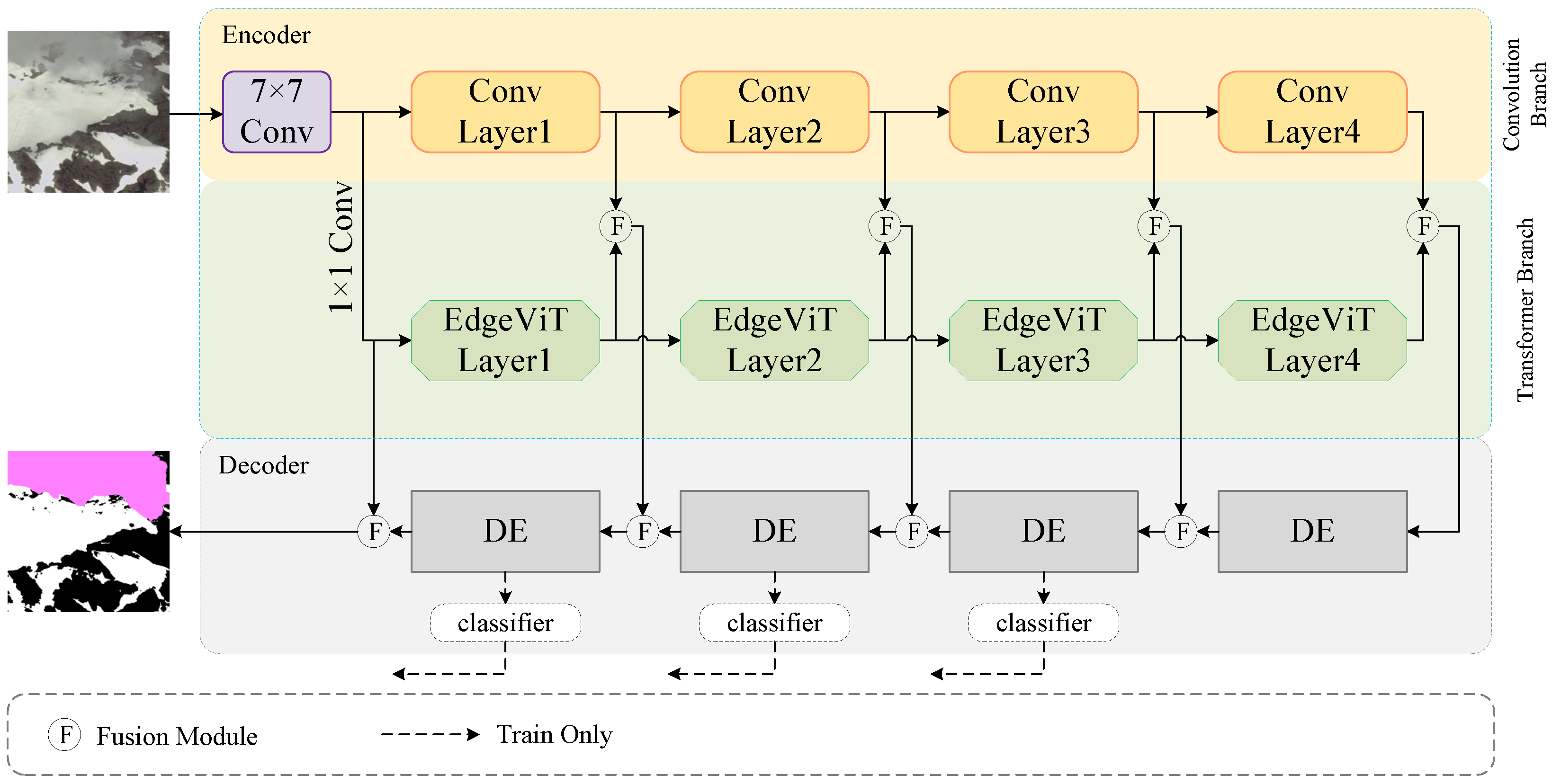Figure 1 shows the whole architecture of the multi-branch convolutional attention network. Furthermore, Algorithm 1 shows the pseudocode of the data transmission process of the multi-branch convolutional attention network. The entire network uses an encoder–decoder design. We believe that the final segmentation accuracy is directly impacted by the precision of feature information extraction [62,63]. Previous studies have proven that convolution is excellent for the extraction of local information, but it lacks accuracy for the grasp of global information. The characteristics of the transformer can make up for this shortcoming. Therefore, a multi-branch mode is adopted in the encoder. The local characteristics of the images are extracted by using a convolution layer, and the transformer layer is used to grasp the global characteristics. After that, the feature data obtained from the two branches are effectively fused. The current fusion strategy just applies a straightforward linear splicing operation on the generated feature map, which is unable to retrieve the useful information. At the same time, the simple splicing operation can easily produce information redundancy, which is extremely unfavorable for the subsequent decoding operation. The integration module is introduced here, which can effectively combine the local and global information extracted from the two branches and filter it, only retaining the meaningful part of it, and it can improve the model efficiency.

In the decoding phase, the majority of modern networks directly upsample to return the original picture size. This can easily cause information loss during upsampling. Some networks use only a single convolution to decode the feature map, and some important feature information is preserved, but the convolution only focuses on local features and cannot establish long-distance connections in the feature map, so the recovery of large-scale cloud/snow areas is not ideal. This paper proposes a new decoder. Combining convolution with atransformer, the effective information in the deep feature is restored gradually. Because the high-level semantic information and spatial information in the upsampling process usually cause the final segmentation boundary to be rough, at the decoder, we again fuse the high-level feature map with the various levels of fusion feature data that the encoder has obtained, so that the important detail information can be retained to achieve an accurate segmentation of clouds/snow.

To increase the accuracy of the final segmentation result, the classifier module is added to the network, which is mainly composed of upsampling and convolution modules. Different levels of output characteristic graphs are drawn at the decoding end to calculate the auxiliary loss, which is used to accelerates the network’s convergence and increase prediction accuracy. The addition of the output strip convolution makes the final output prediction map more refined.

Algorithm 1 The data-transmission process of MCANet

Input:  Training data: D = {($x_1$, $y_1$), ($x_2$, $y_2$), …, ($x_m$, $y_m$)}; Attribute set: A Output:  The final segmentation picture: $Ou{t}_1$ = classifier(F($D_1$, $X_1$)) and $Ou{t}_i=classifier\left(D_i\right)$, i = 2, 3, 4 1: The backbone network extracts features, and the backbone network routing convolution branch and attention branch are constituted 2: The convolution branch extracts features and outputs feature maps of different levels: $X=\{X_1,X_2,X_3,X_4,X_5\}$ 3: The transformer branch extracts features and outputs feature maps of different levels: $Y=\{Y_2,Y_3,Y_4,Y_5\}$ 4: The features of different branches are fused, $Q_i=F(X_i,Y_i)$, i = 2, 3, 4, 5, and the output is obtained: $Q=\{Q_2,Q_3,Q_4,Q_5\}$ 5: The high-level features are upsampled and passed through the decoder module: $D_5=DE\left(Q_5\right)$ 6: for i = 5,4,3,2 do 7:     Fusion of shallow features and deep features: $F_i=F(Q_{i-1},D_i)$ 8:     Through the decoder module: $D_i=DE\left(F_i\right)$ 9:     if i! = 5 then 10:         The output is obtained: $Ou{t}_i=classifier\left(D_i\right)$ 11:     end if 12: end for 13: return$Ou{t}_1$ = classifier(F($D_1$, $X_1$)) and $Ou{t}_i=classifier\left(D_i\right)$, i = 2, 3, 4

2.2. Backbone

Because clouds and snow have similar spectral characteristics and color attributes [52], they are easily disturbed by complex underlying surfaces. A single convolution or transformer structure does not meet the need for feature extraction in cloud/snow images. We use the multi-branch structure of convolution and transformer as the backbone of the model to abstract the characteristic information of the image. Convolution extracts features by sharing convolution kernels to reduce network parameters and to improve model efficiency, and its translation invariance makes feature detection for images more sensitive, but its limited receptive field makes it less capable of extracting global information. However, the emergence of transformers enables the global information in the image to be captured, and transformers have shown phenomena beyond those of CNN in many visual tasks. In this study, we combine the benefits of transformer and convolution to extract different levels of characteristic information, which perfectly inherits the advantages of convolution and transformer, so as to enhance the model’s capacity for feature extraction.

Table 1. The architecture of the network.

Levels	Convolution Branch	Guidance Module	Transformer Branch	Decoder	Size
L1	7 /times 7, 64, stride = 2	⟶ 1 /times 1, 48, stride = 1		Classifier	1/2
L2	$\left[\begin{array}{c}3\times 3,64,stride=1\hfill \\ 3\times 3,64,stride=1\hfill \end{array}\right]\times 3$	⟶ fusion ⟵	EdgeViT_block (dim = 96, heads = 1) × 1	DE1	1/4
L3	$\left[\begin{array}{c}3\times 3,128,stride=1\hfill \\ 3\times 3,128,stride=1\hfill \end{array}\right]\times 4$	⟶ fusion ⟵	EdgeViT_block (dim = 240, heads = 2) × 2	DE2	1/8
L4	$\left[\begin{array}{c}3\times 3,256,stride=1\hfill \\ 3\times 3,256,stride=1\hfill \end{array}\right]\times 6$	⟶ fusion ⟵	EdgeViT_block (dim = 384, heads = 4) × 3	DE3	1/16
L5	$\left[\begin{array}{c}3\times 3,512,stride=1\hfill \\ 3\times 3,512,stride=1\hfill \end{array}\right]\times 3$	⟶ fusion ⟵	EdgeViT_block (dim = 384, heads = 8) × 2	DE4	1/32

shows the specific structural parameters of the model.

As we can see in Figure 2a, we use two layers of 3 × 3 convolutions as the block of our convolution branch. Algorithm 2 shows the pseudocode of the data transmission process of the convolution branch block. The addition of the residual structure makes the model lessen the rate of information loss, and it can protect the integrity of information when extracting features. The convolution branch’s computation procedure can be stated as follows:

$$C=\sigma (BN\left(Con{v}_{3\times 3}\left(f_i\right)\right),$$

(1)

$$f_{i+1}=\sigma (BN\left(Con{v}_{3\times 3}\left(C\right)\right),$$

(2)

where $f_i$ and $f_{i+1}$ represent the i-th layer input and output of the convolution branch, respectively; BN (.) represents batch normalization, $\sigma$ (.) is a representation of the nonlinear activation function ReLU; and $Co{n}_{3\times 3}$ (.) is a representation of the 3 × 3 convolution operation.

Algorithm 2 Data transmission process of the convolution branch block

Input:  The output feature map of the previous layer: $f_i$ Output:  $f_{i+1}$ 1: $C=\sigma (BN\left(Con{v}_{3\times 3}\left(f_i\right)\right)$ 2: $f_{i+1}=\sigma (BN\left(Con{v}_{3\times 3}\left(C\right)\right)$ 3: return$f_{i+1}$

For the transformer branch, considering the number of parameters and the computational complexity of the model, we use the block in EdgViTs [58] as the component part of our transformer branch. EdgViTs is a new lightweight ViT family, and it is achieved by introducing a high-cost local–global–local (LGL) information exchange bottleneck based on the optimal integration of self-attention and convolution. The particular structure is displayed in Figure 2b, and Algorithm 3 shows the pseudocode of the data transmission process of the transformer branch block. It mainly includes three operations: (1) local aggregation, utilizing effective depthwise convolutions, local information aggregation from neighbor tokens (each corresponding to a distinct patch); (2) global sparse attention, generating a sparse collection of regularly spaced delegate tokens for distant information exchange via self-attention; and (3) local propagation, using transposed convolutions to spread updated information from delegate tokens to non-delegate tokens in nearby areas. The main calculation process can be expressed as follows:

$$X=LocalAgg\left(Norm\left(X_{in}\right)\right)+X_{in},$$

(3)

$$Y=FFN\left(Norm\right(X\left)\right)+X,$$

(4)

$$Z=LocalProp\left(GlobalSparseAttn\right(Norm\left(Y\right)\left)\right)+Y,$$

(5)

$$X_{out}=FFM\left(Norm\left(Z\right)\right)+Z,$$

(6)

where $X_{in}$ $ϵ$ $R^{H\times W\times C}$ denotes the input tensor, Norm (.) denotes Layer Normalization, LocalAgg (.) denotes the local aggregation operator, FFN (.) denotes the perceptron with two layers, GlobalSparseAttn (.) denotes global sparse self-attention, and LocalProp (.) denotes global sparse self-attention.

Algorithm 3 Data transmission process of the transformer branch block

Input:  The output feature map of the previous layer: $X_{in}$ Output:  $X_{out}$ 1: $X=LocalAgg\left(Norm\left(X_{in}\right)\right)+X_{in}$ 2: $Y=FFN\left(Norm\right(X\left)\right)+X$ 3: $Z=LocalProp\left(GlobalSparseAttn\right(Norm\left(Y\right)\left)\right)+Y$ 4: $X_{out}=FFM\left(Norm\left(Z\right)\right)+Z$ 5: return$X_{out}$

Because of the restriction of the receptive field, the perception of the objective in the picture is always limited. To enlarge the receptive field, dilated convolution can be applied to the current method, but considering the complexity of remote sensing image content, a single use of the convolution operation makes large-scale targets, and the small-scale cloud/snow area is always impossible to take into account, so the transformer branch joins the perfect solution to this problem. The two branches complement each other, taking into account the extraction of small targets and the effective identification of large-scale clouds/snow, and self-attention enables the effective learning of global information and long-distance dependencies. This is useful for avoiding the interference of similar color attributes of cloud and snow, so that the model can effectively distinguish cloud and snow.

2.3. Fusion Module

Clouds and snow have complex edge shapes relative to other targets. Accurately restoring the edge features of clouds and snow has always been a difficult task. In addition, the feature maps produced by different layers of the model will provide an enormous amount of useless information. Filtering this information is particularly important. If the information contained in the feature map cannot be fully integrated, the noise and other factors contained in it will have a huge influence on the final categorization outcomes.

To solve the problems described above, we suggest a fusion module to fuse the information from different layers. In the backbone, the different levels of features abstracted by the convolution branch and the transformer branch need to establish a complementary relationship in order for the model to perfectly inherit the benefits of convolution and the transformer. At the decoder level, the category information with rich high-level characteristics can direct the classification of low-level characteristics, while the location information retained by the low-level features can supplement the spatial location information of the high-level characteristics. 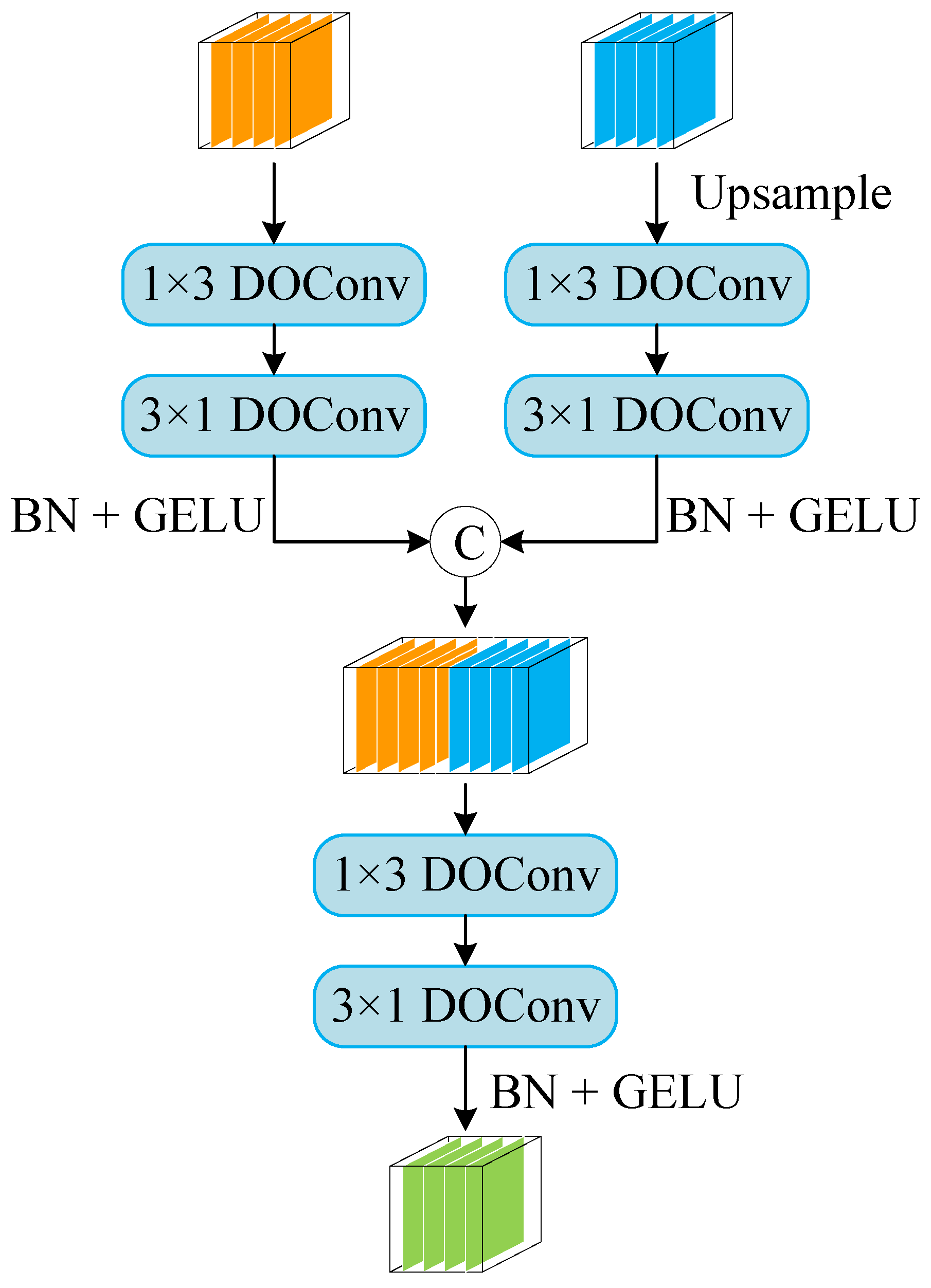Figure 3 demonstrates the general layout of the fusion module that is proposed in this study, and Algorithm 4 shows the pseudocode of the data transmission process of Fusion Module. In this module, we use DO-Conv [64] to replace the traditional convolution. DO-Conv is a depthwise over-parameterized convolutional layer that adds learnable parameters, which has positive significance for many visual tasks.

Algorithm 4 Data transmission process of the Fusion Module

Input:  Feature maps of different levels in our network: $X_{in1}$ and $X_{in2}$ Output:  $Y_{out}$ 1: $X_1=G\left(BN\left(DOCon{v}_{3\times 1}\left(DOCon{v}_{1\times 3}\left(X_{in1}\right)\right)\right)\right)$ 2: $X_2=G\left(BN\left(DOCon{v}_{3\times 1}\left(DOCon{v}_{1\times 3}\left(Up\left(X_{in2}\right)\right)\right)\right)\right)$ 3: $W=Concat(X_1,X_2)$ 4: $Y_{out}=G\left(BN\left(DOCon{v}_{3\times 1}\left(DOCon{v}_{1\times 3}\left(W\right)\right)\right)\right)$ 5: return $Y_{out}$

The use of stripe convolution enables the model to more effectively extract the edge features of clouds and snow. As far as we can see in the figure, there are two parallel branches that make up the fusion module. Firstly, the deep-level features are amplified to the same level as the low-level features of another branch, and then the strip convolution is used to filter the information in the deep-level features and the low-level features, and enhance the feature extraction ability. The strip convolution architecture is mainly composed of two convolution kernels with sizes of 1 × 3 and 3 × 1, a batch normalization layer, and an activation function GELU [65]. Then, the information abstracted by two branches is combined and finally sent to the next level of the network after the action of two layers of the strip convolution layer. The calculation process is as follows:

$$X_1=G\left(BN\left(DOCon{v}_{3\times 1}\left(DOCon{v}_{1\times 3}\left(X_{in1}\right)\right)\right)\right),$$

(7)

$$X_2=G\left(BN\left(DOCon{v}_{3\times 1}\left(DOCon{v}_{1\times 3}\left(Up\left(X_{in2}\right)\right)\right)\right)\right),$$

(8)

$$W=Concat(X_1,X_2),$$

(9)

$$Y_{out}=G\left(BN\left(DOCon{v}_{3\times 1}\left(DOCon{v}_{1\times 3}\left(W\right)\right)\right)\right),$$

(10)

$X_{in1}$ and $X_{in2}$ represent the two inputs of the fusion module, $Y_{out}$ represents the output, $DOCon{v}_{n\times m}$ (.) represents the convolution procedure using an n × m convolution kernel, Up (.) represents the bilinear interpolation upsampling operation, Concat (.) represents the splicing operation based on the channel dimension, and BN (.) and G (.) represent batch normalization and the nonlinear activation function GELU. The use of the GELU activation function to replace the traditional ReLU is due to the idea of random regularization added to GELU, which improves the network accuracy.

2.4. Decoder Module

The distribution characteristics of cloud and snow are not uniform in distribution, and the shape is complex and changeable. Similar color attributes also make it more difficult to distinguish them. The interference of a complex background often causes the phenomenon of misjudgment or omission. During the upsampling procedure, the current methods often directly decode the high-level feature map or use a single convolution to decode the feature map and restore the original image features. This will make the model lose information due to the wrong attention to feature information throughout the upsampling phase, which makes it challenging to recover the details. As a result, the model cannot correctly differentiate between clouds and snow, and it is susceptible to misjudgment due to interference from complex backgrounds.

We provide a new decoder module as a solution to the aforementioned issues. Inspired by Xia X et al. [66], who previously proposed that a complementary convolution and transformer can make up for the deficiency of single use, the scheme of combining the CNN and transformer is adopted to construct a hybrid module that is composed of convolution and a transformer, to significantly increase the efficiency of information flow. As we can see in Figure 4, we first used a 1 × 1 convolution layer to modify the quantity of input channels, and then a transformer module is involved to establish a long-distance dependency in the feature map. A channel splitting layer is introduced into the module, and the ratio r is used to adjust the proportion of the convolution module in the hybrid module to further improve the efficiency. We suppose that the amount of the input channel is $C_{in}$, that the amount of the output channel after the transformer module is $C_{out}\times r$, and that the amount of the output channel after the convolution module is $C_{out}\times (1-r)$. Finally, the results of the transformer module and convolution module are concatenated to obtain the final output. The calculation process is as follows:

$$W=Con{v}_{1\times 1}\left(X\right),$$

(11)

$$T=Trans\left(W\right),$$

(12)

$$C=Conv\left(T\right),$$

(13)

$$Y=Concat(T,C),$$

(14)

where $Con{v}_{1\times 1}$ (.) represents the convolution procedure using a 1 × 1 convolution kernel, Trans (.) and Conv (.) represent the passing transformer module and convolution module, respectively, and Concat (.) represents the splicing operation based on the channel dimension. Algorithm 5 shows the pseudocode of the data transmission process of the Decoder Module.

Algorithm 5 Data transmission process of the transformer Decoder Module

Input:  The output feature map of the previous layer: $X_{in}$ Output:  $Y_{out}$ 1: $W=Con{v}_{1\times 1}\left(X_{in}\right)$ 2: $T=Trans\left(W\right)$ 3: $C=Conv\left(T\right)$ 4: $Y=Concat(T,C)$ 5: return $Y_{out}$

2.5. Experiment Details

The PyTorch framework was used for all our expriments. The version number was 1.10.0, and the Python version was 3.8.12. The experimental equipment includes the NVIDIA series graphics card, the graphics card model is NVIDIA GeForce RTX 3060, the graphics memory is 12 G, the CPU is i5-11400, and its computing memory is 16 G.

Due to restrictions on GPU memory, we defined the batch size for each iteration to 4 when using the CSWV Dataset for training, and the training batch size of the other two datasets was set to 8, while the training period was 300 epochs. When training the dataset, we used the equal interval adjustment learning rate (StepLR) strategy. As the number of training epochs increased, the learning rate was reduced accordingly to achieve better training results. In the initial stage of training, the learning rate was set to 0.00015, the attenuation coefficient was 0.98, and the learning rate was updated every three epochs. The learning rate for each epoch is calculated as follows:

$${lr}_N={lr}_0·{\beta }^{N/s},$$

(15)

where $l{r}_N$ is the learning rate of the Nth training, $l{r}_0$ is the initial learning rate, $\beta$ is the attenuation coefficient, and s is the update interval.

We chose the cross-entropy loss function as the loss function of model training, and the calculation formula of the loss function is as follows:

$$Loss(x,class)=-log\left(\frac{e^{x\left[clas\right]}}{{\sum }_i{e}^{x\left[i\right]}}\right)=-x\left[class\right]+log\left({\sum }_i{e}^{x\left[i\right]}\right),$$

(16)

where x is the output tensor of the model, and class is the real label.

As the traditional adaptive learning-rate optimizer (including Adam, RMSProp, etc.) faces the risk of falling into bad local optimization, we used the RAdam optimizer [67] as our optimizer. RAdam provides a dynamic heuristic to provide automatic variance attenuation, and it is more robust to changes in learning rate than other optimizers. It can provide a better training accuracy and generalization ability in various datasets, and brings better training performance to the model.

To improve the model’s capacity for generalization, and to prevent overfitting during training, we also performed data augmentation on the dataset. Because clouds and snow have similar color properties, in addition to randomly rotating and flipping the image, the contrast, sharpening, brightness, and color saturation of the image were randomly adjusted with a probability of 0.2 during training.

For the purpose of assessing the model’s real performance, this paper introduces the evaluation indexes of pixel accuracy (PA), mean pixel accuracy (MPA), F1, frequency weighted intersection over union (FWIOU), and mean intersection over union (MIOU) to evaluate the performance of the model in practical applications. Their calculation formulas are as follows:

$$P=\frac{p_{ii}}{p_{ii}+p_{ij}},$$

(17)

$$R=\frac{p_{ii}}{p_{ii}+p_{ji}},$$

(18)

$$F_1=2·\frac{P·R}{P+R},$$

(19)

$$PA={\displaystyle \sum _{i=0}^k}\frac{P_{ii}}{{\displaystyle \sum _{j=0}^k}{P}_{ij}},$$

(20)

$$MPA=\frac{1}{k+1}{\displaystyle \sum _{i=0}^k}\frac{p_{ii}}{{\displaystyle \sum _{j=0}^k}{p}_{ij}},$$

(21)

$$FWIOU=\frac{1}{{\displaystyle \sum _{i=0}^k}{\displaystyle \sum _{j=0}^k}{p}_{ij}}{\displaystyle \sum _{i=0}^k}\frac{{\displaystyle \sum _{j=0}^k}{p}_{ij}{p}_{ii}}{{\displaystyle \sum _{j=0}^k}{p}_{ij}+{\displaystyle \sum _{j=0}^k}{p}_{ji}-p_{ii}},$$

(22)

$$MIOU=\frac{1}{k+1}{\displaystyle \sum _{i=0}^k}\frac{p_{ii}}{{\displaystyle \sum _{j=0}^k}{p}_{ij}+{\displaystyle \sum _{j=0}^k}{p}_{ji}-p_{ii}},$$

(23)

where P is Precision, which represents the probability that the pixels in the prediction result are predicted correctly; R is the recall rate Recall, which represents the probability that the pixels in the true value are predicted correctly; k stands for the number of classes (excluding the background scene); $p_{ii}$ identifies the number of pixels in category i and predicted as category i; $p_{ij}$ is the number of pixels in category i that are predicted to be in category j; and $p_{ji}$ is the number of pixels in category j that are predicted to be in category i.

3. Experiment

3.1. Datasets

3.1.1. CSWV Dataset

Due to the small number of high-resolution cloud and snow datasets, we used a WorldView2-based cloud/snow dataset (CSWV) constructed by Zhang [52], and used it as our main dataset. This is the first free high-resolution remote sensing image dataset for cloud and snow detection. Data sources are available from [52]. Its spatial resolution is mainly 0.5–10 m, including 27 high-resolution images of clouds and snow from remote sensing. The shooting location was mainly in the Cordillera Mountains in North America, and the time distribution was from June 2014 to July 2016. The background in the picture is complex and diverse, including forest, grassland, lake area, and bare land. The types of clouds include cirrus, altocumulus, cumulus, and stratus. Snow mainly includes permanent snow, stable snow, and discontinuous snow. The diversity of cloud and snow types makes the dataset more generalized and representative.

We believe that larger pictures are beneficial to the training of the model. Considering the limitation of the device, the original picture of the large scene is cut to 512 × 512 size. In order to make the training data more reasonable, we filter the clipped images, delete the pictures with full cloud and full snow, or no cloud and no snow, and finally obtain 3000 pictures. Then, all the pictures are randomly divided into training set and verification set according to the ratio of 8:2. Some of the training set images are shown in Figure 5. The top line contains the original color image, with the background from left to right being forest, lake, grass, town, bare land, and mountains. The second row is the corresponding label, where the cloud is represented by pink, the snow is represented by white, and the background is represented by black.

3.1.2. HRC_WHU Dataset

In order to test the generalization performance of our method, we used the high-resolution cloud cover dataset HRC_WHU [68] for verification. Data sources are available from [68]. The dataset was created by theSENDIMAGE laboratory at Wuhan University. It contains 150 high-resolution remote sensing images of large scenes. Each image contains three-channel RGB information, distributed in various regions of the world, including vegetation, snow, desert, urban, and water. There are five different backgrounds. The image resolution is mainly between 0.5 meters and 15 meters. The original size of image was 1280 × 720. Because of the memory constraints of the GPU, we cut the original images into small 256 × 256 images for training. Finally, 3000 images were obtained, and then all images were randomly divided into training set and verification set according to the ratio of 8:2. Some of the pictures in the training set and their labels are shown in Figure 6. From left to right, the background is desert, snow, urban area, vegetation, and water area. The top row is the original picture, and the second row is the corresponding label. The cloud is represented by white, and the background is represented by black.

3.1.3. Cloud and Cloud Shadow Dataset

This dataset mainly includes images taken from Landsat8 satellite and high-resolution remote sensing image data selected from Google Earth (GE). The Landsat8 satellite carries a total of 11 bands of land imagers and thermal infrared sensors, of which band 2, band 3, and band 4 are used. GE contains high-definition satellite images from all over the world, mainly from the QuickBird satellite and the WorldView series satellite, with three bands of channel information and a spatial resolution of 30 meters. Because the size of the image obtained directly was too large, the size of the image taken by the Landsat8 satellite was 10,000 × 10,000, and the size of the image obtained on GE was 4800 × 2742. Limited by GPU memory, the original image was uniformly cut to 224 × 224 for training. After cutting, we obtained a total of 10,000 pictures. Then, we randomly divided all the pictures into training set and verification set according to the ratio of 8:2.

To guarantee that the dataset is genuine and representative, the images we selected contain multiple different angles, heights, and backgrounds. The image background mainly includes different scenes such as woodland, desert, urban areas, farmland, etc., as shown in Figure 7. Some images were selected to display. From left to right, the background is the urban area, woodland, desert, water area, farmland, and mountain; the first row is the original picture; and the second row are their corresponding labels. The cloud is symbolized by red, the cloud shadow is symbolized by green, and the background is symbolized by black.

3.1.4. Landsat8 SPARCS (L8 SPARCS)

This is a cloud and snow dataset created by M. Joseph Hughes of Oregon State University [69,70]. The images were captured by the Landsat8 satellite, which is equipped with two types of sensors: land imager (OLI) and thermal infrared sensor (TIRS). The dataset mainly includes 80 remote sensing image data points of different scenes of 1000 × 1000 size, which are classified into five categories: cloud, cloud shadow, snow/ice, water, and background. We cut the original image into 256 × 256 small pictures for training. Then, all images are randomly divided into the training set and validation set, according to the ratio of 8:2. Figure 8 shows some data in the training set. The first line is the original image, and the second line is its corresponding label. The white area represents the cloud, the black area represents the cloud shadow, the sky blue area represents the snow/ice, the dark blue area represents the water area, and the gray area represents the background.

3.2. Ablation Study

On the CSWV Dataset, we conducted ablation tests to confirm the actual effect of each module in the network. Firstly, the convolution branch was directly used as the reference backbone, each layer was directly upsampled, and the feature maps that resulted from each layer were then spliced and output. As shown in

Table 2. Ablation experiments of different modular combinations.

Methods	MIOU(%)
Convolution Branch	91.974
Convolution Branch + Transformer Branch	92.420 (0.446 ↑)
Convolution Branch + Transformer Branch + Fusion Module	92.520 (0.1 ↑)
Convolution Branch + Transformer Branch + Fusion Module + DE	92.736 (0.216 ↑)

, we used MIOU as an evaluation index to evaluate the performance of the model. At this time, the MIOU values of the model were only 91.974%.

Then, each module was ordinally added to the network to test its feasibility and that of the whole model. Table 2 shows the index changes of the whole network after different modules were added in turn. The details in the table show that when all modules are added, the network we proposed has the highest accuracy and achieves the optimal results. To clearly demonstrate the real influence of each module on the entire network, two pictures were extracted from the dataset for visualization experiments. As shown in Figure 9, a picture containing a large-scale cloud layer was selected to show the heat map of the whole network of the cloud after adding different modules. The detection of thin clouds has always been a difficult problem. To demonstrate the effect of each module in this network for detecting thin clouds, a picture with both thin clouds and snow was selected, as shown in Figure 10. Different module combinations were used to generate heat maps for clouds and snow, in which black boxes are used to mark the target areas with significant differences in attention.

The multi-branch ablation experiment: In order to meet the requirements of complex feature extraction, a single convolution or transformer cannot fully extract the features of clouds and snow. The multi-branch structure proposed in this paper combines convolution with a transformer. The convolution branch is used to extract local feature information, as well as small-scale cloud and scattered snow information. The transformer branch can establish the dependence relationship between long-distance information in the image, which is beneficial for the large-scale extraction of cloud/snow information. At the same time, global attention greatly reduces the interference of the extraction of complex background-to-feature information. Additionally, the attention mechanism causes the model to focus more on the objective. As we can see in Figure 9b,c, after the transformer branch is added, the model pays more attention to the cloud. As shown in Figure 10b,c this also demonstrates that the network of the multi-branch structure and the single convolution branch has obvious differences in the attention of cloud and snow. After the transformer branch is added, more attention is paid to the target. Table 2 demonstrates that the MIOU value of the network reaches 92.420% after the multi-branch structure is used, which is 0.446% higher than when only the convolution branch is used.

The ablation experiment of the fusion module: Our purpose in constructing this module is to fuse the information between different feature maps of the convolution branch and the transformer branch. In the decoding process, the information between each of the high-level features and low-level features is guided through the fusion module, and the meaningful information between different feature maps is filtered out, which helps to increase the recognition effectiveness and increase the model’s capacity for recognition. The use of strip convolution makes the model more precise in image segmentation. Figure 9 and Figure 10c,d show that the image segmentation is more refined, while the target attention is improved, after the fusion module is added. Table 2 shows that the MIOU value of the whole model reaches 92.520% after this fusion module is added, which is 0.1% higher than that before it is added.

The ablation experiment for the decoder module: In the decoding part of the model, a decoder module was reconstructed. Mixing the convolution with transformer is more effective than a single convolution or transformer alone, and doing so keeps more of the image’s original characteristics. Meanwhile, due to the addition of the transformer, the model does not reduce the attention to the targets during the decoding process. On the contrary, the discrimination between the target and the background is more obvious. The discrimination between cloud and background shown in Figure 9e is more obvious than that without this module. Figure 10e shows the heat maps of cloud and snow in the same image after this decoder module is added. To the left of the picture, there is a thin cloud, and it has similar characteristics with the underlying surface, which are easy to confuse. After this decoder module was added, the network suggested in this article was capable of accurately identifying thin clouds from the underlying surface, and the discrimination between target and background was more obvious.

3.3. Comparison Test of the CSWV Dataset

In this part, to test the actual performance of our model, it is contrasted with other excellent models from the past five years, namely DFANet [71], CVT [57], DABNet [72], and HRNet [73]. To be able to highlight the advantages of our model in cloud/snow detection tasks, we also used excellent models dedicated to cloud/snow detection in recent years as controls for comparative experiments. The contrast network used in this paper has its own characteristics. For example, FCN8s uses a fully convolutional structure to achieve pixel-level classification. In DFANet, a semantic segmentation coding module with multiple connection structures is embedded. DenseASPP [45] uses a densely connected structure. PVT introduces the pyramid structure into transformer in order to gradually lower the feature map and to make it acceptable for challenging prediction tasks. PAN [74] added a bottom-up pyramid, enabling low-level positioning features to be passed over so that the model can gather semantic and location information from the picture. For immediate semantic segmentation, BiseNetV2 [75] uses a two-branch structure to collect spatial and semantic information. For the cloud/snow detection task, PADANet [50] used a parallel approach where two branches were involved in the calculation to enhance the precision and speed of the model. MSPFANet [76] proposed a multi-scale banded pooling module to enhance the edge-segmentation capability. In CSDNet [52], multi-scale feature fusion was used to increase the detection percision and detection efficiency of cloud/snow. In SP_CSANet [77], the strip pooling residual structure and attention module are used to avoid background interference.

Table 3. Comparison of evaluation indexes of different models on the CSWV Dataset (the network dedicated to cloud/snow detection is marked in italics, and the best results are displayed in bold).

Method	PA (%)	MPA (%)	F1 (%)	MIOU (%)	FWIOU (%)
DFANet [71]	95.239	91.057	88.926	85.368	91.206
DenseASPP (MobilenetV2) [45]	96.129	94.067	90.295	87.875	92.655
SegNet [79]	96.381	94.335	90.512	88.173	93.143
BiseNetV2 [75]	96.476	93.611	91.414	88.724	93.337
PADANet [50]	96.787	94.158	92.070	89.596	93.912
OCRNet [46]	96.791	94.643	91.947	89.678	93.912
PVT [56]	96.836	94.514	92.162	89.82	94.017
ESPNetV2 [80]	96.814	94.234	92.417	89.955	93.970
DABNet [72]	96.827	95.087	92.118	90.030	93.943
ACFNet (resnet50) [81]	96.778	95.536	91.924	90.040	93.823
GAFFRNet (resnet18) [51]	96.974	94.893	92.535	90.350	94.240
PSPNet (resnet50)  [43]	97.024	94.619	92.834	90.504	94.316
ENet [44]	97.026	95.237	92.591	90.555	94.305
CCNet (resnet50) [82]	97.093	94.957	92.744	90.572	94.431
MSPFANet (resnet18) [76]	97.079	95.059	93.024	90.891	94.448
FCN8s (vgg16)  [40]	97.186	95.643	93.002	91.129	94.608
CSDNet  [52]	97.166	96.033	92.964	91.265	94.563
UNet [41]	97.261	94.697	93.732	91.402	94.801
HRNet [73]	97.254	95.612	93.354	91.447	94.748
PAN (resnet50)  [74]	97.314	95.485	93.477	91.491	94.854
SP_CSANet  [77]	97.307	95.582	93.504	91.581	94.853
CDUNet (resnet50) [78]	97.330	95.838	93.455	91.642	94.892
MCANet	97.650	96.354	94.350	92.736	95.483

displays the score indicators of different networks on the CSWV Dataset. Here, we used PA, MPA, F1, MIOU, and FWIOU as evaluation indicators to assess the effectiveness of each model. It is visible from the table that for cloud/snow detection, the model suggested in this paper has the highest detection precision and is superior to other networks for all indicators. The scores on the five indicators are PA, 97.650%; MPA, 96.354%; F1, 94.350%; MIOU, 92.736%; and FWIOU, 95.483%. In other models, CDUNet [78] introduces multi-scale convolution and high-frequency feature extractors to improve cloud borders and to forecast debris clouds. A dual attention mechanism also makes it better for cloud/snow detection, so that the detection accuracy is second only to the model proposed in this paper. Other models use a pure convolution structure or add an attention mechanism to convolution, but the final results are all not ideal. Although PVT uses a combination of convolution and a transformer, its MIOU value on cloud/detection tasks is only 89.82%, which is far less than our model.

To exhibit our model’s benefits for cloud and snow detection tasks, we selected several images with different information for prediction. As shown in Figure 11, besides the model given in this article, the prediction results of other models are also used for comparison, in which we mark the missed and false detection areas in the figure with red boxes. The images we selected contained different backgrounds, including bare land, vegetation, water area, and desert. Many kinds of clouds include both thick and thin clouds. The fragmented distribution of snow also makes the detection much more challenging. We can see in the figure that the segmentation result of PSPNet and BiseNetV2 is the roughest. Seeing as the color characteristics of clouds and snow are similar, discerning them is significantly harder to than with other tasks. BiseNetV2 cannot accurately differentiate clouds and snow, and there are a lot of false detections. Due to the addition of the pyramid pooling structure, PSPNet has a certain degree of improvement in the detection of targets of different scales in theory, but it is susceptible to complex background interference for cloud/snow tasks. As shown in the fifth set of images, PSPNet is completely unable to detect snow on wasteland. Although the detection effect of HRNet and SP_CSANet is improved to a certain extent, and it can accurately distinguish between clouds and snow, there are still some missed detections in some areas with thin clouds, and the ability to recover the edge details of clouds needs to be improved. Our model uses a convolution branch and a transformer branch to extract local and global features in the image and combine them to complement each other. The multi-branch structure enables us to completely extract the hidden information in the image, avoiding the interference of similar color attributes of clouds and snow, and accurately locate the clouds and snow. The addition of a new fusion module can accurately combine information in feature maps of different scales. As the figure illustrates, our model can not only accurately locate the cloud/snow location, but small-scale thin clouds can also be effectively detected. In addition, the ability to recover the edge of the cloud is much stronger than the model used for comparison, and the boundary of the target can be accurately segmented. The final prediction result is the most realistic.

Figure 12 demonstrates the segmentation impact of several models on the cloud’s edge. We use green lines to outline the edge of the cloud segmented using different models. The graph shows that our model creates a new fusion module to combine various levels of information, and adds strip convolutions inside, so that the detail recovery of the cloud edge is the closest to the actual situation and it can perfectly fit the edge of the cloud. Other models such as BiseNetV2 and SP_CSANet not only recognize non-cloud backgrounds as clouds, but they also handle cloud boundaries roughly. In general, our method can restore the real situation of the cloud boundary as much as possible, and the segmentation results are more suitable for the cloud boundary than with other models.

Since the locations of the images collected are different, and the interference information contained in the background varies, the segmentation effect of each model on the cloud/snow under a relatively complex background is shown in Figure 13 to further test the performance of our model under complex background interference. The first group and the second group of pictures in the picture are collected in the rock gravel area, and the distributed cloud layer are also thin clouds that are difficult to detect. The third group of pictures are collected on the bare wasteland, and the bare ground has similar characteristics to the thin snow covered, which can easily interfere with the snow detection of the model. The road in the fourth group of images is easily misjudged as snow. The distribution of clouds and snow in the fifth group of images is extremely fragmented, coupled with a large amount of noise, which greatly increases the difficulty of model detection.

From Figure 13, it is clear that in the first set of pictures, HRNet misjudged the white rock and soil as snow. In the second group of images, because the cloud layer is too thin, the color discrimination between it and the underlying surface is not obvious, so that other models cannot accurately locate the cloud position, and more or less misjudgment will occur. For the fourth group of images, HRNet and BiseNetV2 misjudged parts of roads as snow, while PSPNet did not detect snow. In the last set of images, due to the very complex distribution structure of clouds and snow, and the large amount of noise interference, neither PSPNet nor BiseNetV2 could accurately segment the shape of clouds/snow, and the segmentation effect was very rough. Although SP_CSANet and HRNet were improved to some extent, they still had false detection due to the interference of background, which led to error-detection and missing-detection phenomena. The method proposed in this paper can avoid the interference of the complex background to a large extent, and it can completely separate the cloud and snow regions from the image. Additionally, the figure illustrates that our model can still generate the best segmentation results in the case of a large amount of interference factors.

3.4. Comparison Test of the HRC_WHU Dataset

To further prove the ability of our model to detect clouds, we conducted comparative experiments on the HRC_WHU Dataset.

Table 4. Comparison of evaluation indexes of different models on the HRC_WHU Dataset (the best results are displayed in bold).

Method	PA (%)	MPA (%)	F1 (%)	MIOU (%)	FWIOU (%)
DenseASPP (MobilenetV2)	92.931	92.755	89.422	86.419	86.815
BiseNetV2	93.407	93.372	90.088	87.299	87.630
FCN8s (vgg16)	93.760	93.753	90.596	87.941	88.251
CVT	93.797	93.560	90.690	87.959	88.343
ESPNetV2	93.944	93.675	90.913	88.220	88.608
SegNet	94.107	93.828	91.155	88.516	88.900
UNet	94.322	94.253	91.424	88.950	89.259
ENet	94.354	94.241	91.479	89.000	89.320
PAN (resnet50)	94.544	94.483	91.747	89.358	89.656
PVT	94.584	94.530	91.804	89.433	89.728
OCRNet	94.701	94.823	91.945	89.679	89.922
DeepLabV3Plus (resnet101)	94.736	94.527	92.065	89.686	90.018
DABNet	94.844	94.978	92.153	89.945	90.181
CCNet (resnet5)	94.874	94.948	92.206	89.989	90.239
PSPNet (resnet50)	95.091	95.188	92.520	90.395	90.631
HRNet	95.137	94.999	92.639	90.442	90.736
MCANet	95.773	95.728	93.560	91.649	91.891

displays the outcomes of the experiment. Here, we used PA, MPA, F1, MIOU, and FWIOU to test the actual performance of each model. It is visible from the table that our model has the highest scores on all five indicators, of which the MIOU index is at least 1.207% higher than other models.

Figure 14 displays the segmentation results of the model for clouds in different scenarios. The environments of the images from top to bottom are desert, snow, town, vegetation, and water area. The types of clouds in the picture include thick clouds, thin clouds, and fragmented small clouds. The segmentation result of thin clouds can be seen in the first series of images in the figure. The second group and the third group of images are the results of segmenting thick clouds. The fourth group of images is a mixture of thick clouds and thin clouds. The detection of thin clouds here is highly susceptible to complex background interference. Clouds on the snow easily confuse the judgment of the interference model with snow, and the boundary recovery of fragmented clouds is a huge challenge.

We mark the areas of false and missed detection in the prediction picture with red boxes. From the figure, we can observe that the prediction effect of BiseNetV2 is the roughest, and it cannot completely restore the shape of the cloud. This is because of the insufficient extraction of semantic features. Although CCNet and PVT have a better segmentation effect on thick clouds, they are easily affected by the background, missing the detection of thin clouds and fragmented clouds. PSPNet presents a certain improvement in its capacity to detect thin clouds; however, the final segmentation result is still poorer than our model, and the recovery of the cloud boundary is not perfect. In the detection of clouds, our model achieves the best results. Regarding our model, the multi-branch structure accounts for various information in the image, so as to achieve a better detection and location of clouds. At the same time, the decoder fully utilizes the characteristic information extracted by these two branches to make the boundary of the cloud more fine, and greatly reduce the interference of clutter scenes.

3.5. Comparison Test of the Cloud and Cloud Shadow Dataset

In this part, we use a self-built cloud and cloud shadow dataset to prove the generalization ability of our model.

Table 5. Comparison of evaluation indexes of different models on the Cloud and Snow Dataset (the best results are displayed in bold).

Method	PA (% )	MPA (%)	F1 (%)	MIOU (%)	FWIOU (%)
CVT	94.623	93.409	90.448	87.697	89.861
SegNet	94.882	93.148	90.986	88.091	90.361
DenseASPP(MobilenetV2)	95.362	94.281	91.770	89.314	91.185
ESPNetV2	95.561	94.598	92.074	89.746	91.543
UNet	95.886	94.735	92.667	90.368	92.150
BiSeNetV2	95.918	94.680	92.781	90.453	92.211
DeepLabV3Plus(resnet101)	96.136	95.401	92.945	90.933	92.591
FCN8s	96.146	95.477	93.023	91.038	92.604
PSPNet(resnet50)	96.283	95.719	93.219	91.335	92.855
HRNet	96.511	95.650	93.787	91.846	93.289
DABNet	96.527	95.953	93.689	91.891	93.308
ENet	96.549	95.763	93.803	91.915	93.357
pvt_s	96.571	95.906	93.817	91.993	93.394
OCRNet	96.683	95.950	94.017	92.205	93.605
PAN(resnet50)	97.254	96.822	94.995	93.547	94.667
CCNet(resnet50)	97.270	96.632	95.177	93.636	94.704
MCANet	97.839	97.351	96.127	94.894	95.782

shows the test results of different models on this dataset. Here, PA, MPA, F1, MIOU, and FWIOU are used as score indicators to evaluate the performance of each model. For the task of identifying clouds and cloud shadows, our model has the highest score on all indicators compared to other methods. The MIOU score reaches 94.894%, which is at least 1.258% higher than those of other models. According to the outcomes shown in the table, our model not only has excellent segmentation ability for clouds, but it also has good generalization ability on cloud and cloud shadow datasets.

Figure 15 demonstrates the segmentation results of each model on clouds and cloud shadows in different scenarios. We selected images in different regions. Images of the first and second sets were captured in desert areas, images of the third sets were clouds and shadows over farmland, the fourth and fifth picture sets were captured over towns, and the sixth and seventh picture sets were captured over vegetation. In the displayed pictures, vegetation and cloud shadow have similar characteristics, which can interfere with the detection of cloud shadows. The fourth group of pictures contains a lot of noise, which also makes the detection much more challenging. Owing to a series of problems such as the insufficient extraction of image information and the loss of information in the upsampling process, other models are easily affected by interference factors, resulting in different degrees of missing detection and erroneous detection. We used the yellow box in the figure to mark where the error was detected. The first and second group of images shows that CVT and BiseNetV2 have many missed detections due to the scattered distribution of cloud shadows. In the fourth set of images, PSPNet misjudged a large number of backgrounds as clouds due to noise interference, and other models were significantly less detailed than the methods proposed in this paper for small edge clouds. The sixth and seventh groups were affected by vegetation. Most models have a rough description of the cloud shadow edge, and CVT did not detect the small cloud in the seventh group of images. In summary, in the final prediction results, the method we suggest can accurately locate the position of clouds and cloud shadows and restore their complete shapes. It can also avoid the interference of similar backgrounds to detect small-scale thin clouds. The anti-interference ability of noise is also significantly better than those of other networks. The overall performance on this dataset is also better than the most advanced network.

3.6. Comparison Test of the L8 SPARCS Dataset

In order to verify the performance of the proposed model in more complex scenarios, the L8 SPARCS Dataset is used for comparative experiments to verify the performance of our proposed method in multi-classification scenarios. Here, we also use PA, MPA, F1, MIOU, and FWIOU as our evaluation indicators to evaluate the performance of the model.

Table 6. Comparison of evaluation indexes of different models on the L8 SPARCS Dataset (the best results are displayed in bold).

Methods	PA (%)	MPA (%)	F1 (%)	MIOU (%)	FWIOU (%)
DenseASPP(MobilenetV2)	85.403	74.929	72.250	65.421	76.496
ENet	86.759	79.685	73.983	68.384	77.649
CVT	87.414	79.125	74.341	68.689	79.117
BiSeNetV2	87.474	79.749	75.613	69.914	79.058
ESPNetV2	88.332	81.228	77.098	71.631	80.173
SegNet	89.324	82.584	78.652	73.306	81.519
DABNet	89.680	84.288	78.288	73.618	81.988
CCNet(resnet50)	89.961	82.704	79.130	73.719	82.583
PSPNet(resnet50)	89.713	81.923	79.673	73.869	82.320
DeepLabV3Plus(resnet101)	89.711	83.992	79.834	74.706	82.351
pvt_s	90.301	85.685	79.535	75.300	82.961
OCRNet	90.441	85.199	80.944	76.113	83.141
PAN(resnet50)	90.925	84.171	81.670	76.281	84.023
HRNet	90.774	85.567	81.904	77.103	83.611
FCN8s	91.481	84.187	82.591	77.264	85.154
UNet	91.758	86.519	83.650	78.968	85.304
MCANet	92.599	87.088	84.902	80.253	86.726

shows the evaluation results of different models for this dataset. It can be seen from the table that after other categories are added, our method can still maintain the highest accuracy, and the detection ability of clouds and snow is far more than with other methods. The score on MIOU is 80.253%, which is at least 1.285% higher than other methods.

Figure 16 shows the prediction of different methods on this dataset, in which we mark the obvious error part of the prediction result with a red solid line. The images used for testing contain a wealth of categories, including scattered small clouds, small rivers, large thick clouds, and perennial ice and snow. Due to the complex background, the detection of small targets is a huge challenge. For example, in the first and third images, most other methods have missed the detection of the narrow river in the middle. In the detection of clouds, cloud shadows, and snow, it has been difficult to recover its edges. ESPNetV2, PAN, and other networks have a rough segmentation of edges and cannot restore the details. Although the effect of SegNet has improved, there is a lot of noise in the final prediction map. The network proposed in this paper can detect small rivers, and the ability to segment boundaries is more in line with the actual situation. The detection effect of small clusters of clouds in the second image and in the four-drop image is also far better than those of other methods.

4. Discussion

4.1. Advantages of the Method

The method proposed in this paper has far better performance than other methods in both cloud/snow datasets and generalization experiments, and can effectively segment cloud and snow regions. The experimental results on four datasets prove the advantages of our method. Compared with other methods, the proposed method has higher detection accuracy. We used the multi-branch structure to combine convolution and a transformer to extract the feature information in the image and then combine it. This can not only make up for the limitations of convolution but also improve the efficiency of feature extraction.

The decoder part is different from most methods that directly recover the original image size or use a single convolution for upsampling. We constructed a new decoder module, which combines convolution and a transformer for the first time to enhance the model’s attention to useful information in the process of image restoration. In the upsampling process, it can avoid the loss of effective information and the interference of invalid information. It can maximize the retention of useful information in the feature map and filter useless information. In practical applications, it can deal with various complex scene conditions, and the anti-interference ability of the model is significantly enhanced. The processing ability for complex scenes is much better than the current method, which can accurately detect the cloud/snow area under the interference of complex background. It greatly reduces the problem of error detection and the missed detection of cloud/snow, and it has strong anti-interference ability. In addition to the fusion effect, the fusion module is also beneficial for the extraction of edge feature information.

4.2. Limitations and Future Research Directions

Although our method has the highest detection accuracy, there is still much room for optimization in the parameters of our model. Due to the multi-branch structure, although the characteristic information in the picture can be effectively extracted, the parameters of the model are also increased. In the future, our studies will aim to reduce the parameters of the model, while ensuring accuracy and minimizing the weight of the model. This paper proves that our method is effective for cloud and snow segmentation for optical remote sensing images. In the future, we hope to extend this method to other remote sensing data, such as SAR remote sensing, to improve the universality of different types of data.

5. Conclusions

This paper proposes a multi-branch convolutional attention network to achieve end-to-end cloud/snow segmentation tasks in optical remote sensing images. The method was tested and verified on different datasets. The tests proved that the detection of cloud/snow is effective, and that the model can accurately segment the cloud/snow area in images. The multi-branch network we designed combines convolution and a transformer. Compared with existing methods, the ability to extract features is greatly enhanced. Experiments on four datasets show that our method has not only the highest accuracy, but also a strong generalization performance. Specifically, the MIOU score on the CSWV Dataset is 92.736%, and the MIOU scores on the generalized datasets, the HRC_WHU Dataset, Cloud and Cloud Shadow Dataset, and L8 SPARCS Dataset, reach 91.649%, 94.894%, and 80.253%, respectively, far exceeding other models.

References

1. Marghany, M. Nonlinear Ocean Fynamics: Synthetic Aperture Radar; Elsevier: Amsterdam, The Netherlands, 2021. [Google Scholar]
2. Marghany, M. Advanced Algorithms for Mineral and Hydrocarbon Exploration Using Synthetic Aperture Radar; Elsevier: Amsterdam, The Netherlands, 2021. [Google Scholar]
3. Manolakis, D.; Marden, D.; Shaw, G.A. Hyperspectral image processing for automatic target detection applications. Linc. Lab. J. 2003, 14, 79–116. [Google Scholar]
4. Huete, A.; Didan, K.; Miura, T.; Rodriguez, E.P.; Gao, X.; Ferreira, L.G. Overview of the radiometric and biophysical performance of the MODIS vegetation indices. Remote Sens. Environ. 2002, 83, 195–213. [Google Scholar] [CrossRef]
5. Hunt, E.R., Jr.; Daughtry, C.; Eitel, J.U.; Long, D.S. Remote sensing leaf chlorophyll content using a visible band index. Agron. J. 2011, 103, 1090–1099. [Google Scholar] [CrossRef] [Green Version]
6. Gao, J.; Weng, L.; Xia, M.; Lin, H. MLNet: Multichannel feature fusion lozenge network for land segmentation. J. Appl. Remote Sens. 2022, 16, 016513. [Google Scholar] [CrossRef]
7. Song, L.; Xia, M.; Jin, J.; Qian, M.; Zhang, Y. SUACDNet: Attentional change detection network based on siamese U-shaped structure. Int. J. Appl. Earth Obs. Geoinf. 2021, 105, 102597. [Google Scholar] [CrossRef]
8. Yin, H.; Weng, L.; Li, Y.; Xia, M.; Hu, K.; Lin, H.; Qian, M. Attention-guided siamese networks for change detection in high resolution remote sensing images. Int. J. Appl. Earth Obs. Geoinf. 2023, 117, 103206. [Google Scholar] [CrossRef]
9. Long, J.; Shi, Z.; Tang, W.; Zhang, C. Single remote sensing image dehazing. IEEE Geosci. Remote Sens. Lett. 2013, 11, 59–63. [Google Scholar] [CrossRef]
10. Paltridge, G.W.; CMR, P. Radiative Processes in Meteorology and Climatology; Elsevier: Amsterdam, The Netherlands, 1976. [Google Scholar]
11. Dozier, J. Spectral signature of alpine snow cover from the Landsat Thematic Mapper. Remote Sens. Environ. 1989, 28, 9–22. [Google Scholar] [CrossRef]
12. Zhu, Z.; Woodcock, C.E. Automated cloud, cloud shadow, and snow detection in multitemporal Landsat data: An algorithm designed specifically for monitoring land cover change. Remote Sens. Environ. 2014, 152, 217–234. [Google Scholar] [CrossRef]
13. Bigdeli, B.; Amini Amirkolaee, H.; Pahlavani, P. Deep feature learning versus shallow feature learning systems for joint use of airborne thermal hyperspectral and visible remote sensing data. Int. J. Remote Sens. 2019, 40, 7048–7070. [Google Scholar] [CrossRef]
14. Price, J.C. Spectral band selection for visible-near infrared remote sensing: Spectral-spatial resolution tradeoffs. IEEE Trans. Geosci. Remote Sens. 1997, 35, 1277–1285. [Google Scholar] [CrossRef]
15. Maglione, P.; Parente, C.; Vallario, A. Coastline extraction using high resolution WorldView-2 satellite imagery. Eur. J. Remote Sens. 2014, 47, 685–699. [Google Scholar] [CrossRef]
16. Gleyzes, M.A.; Perret, L.; Kubik, P. Pleiades system architecture and main performances. Int. Arch. Photogramm. Remote Sens. Spat. Inf. Sci. 2012, 39, 537–542. [Google Scholar] [CrossRef] [Green Version]
17. Sun, L.; Mi, X.; Wei, J.; Wang, J.; Tian, X.; Yu, H.; Gan, P. A cloud detection algorithm-generating method for remote sensing data at visible to short-wave infrared wavelengths. ISPRS J. Photogramm. Remote Sens. 2017, 124, 70–88. [Google Scholar] [CrossRef]
18. Warren, S.G. Optical properties of snow. Rev. Geophys. 1982, 20, 67–89. [Google Scholar] [CrossRef]
19. Allen, R.C., Jr.; Durkee, P.A.; Wash, C.H. Snow/cloud discrimination with multispectral satellite measurements. J. Appl. Meteorol. Climatol. 1990, 29, 994–1004. [Google Scholar] [CrossRef]
20. Moses, W.J.; Philpot, W.D. Evaluation of atmospheric correction using bi-temporal hyperspectral images. Isr. J. Plant Sci. 2012, 60, 253–263. [Google Scholar] [CrossRef]
21. Liu, X.; Xu, J.M.; Du, B. A bi-channel dynamic thershold algorithm used in automatically identifying clouds on gms-5 imagery. J. Appl. Meteorlog. Sci. 2005, 16, 134–444. [Google Scholar]
22. Tapakis, R.; Charalambides, A. Equipment and methodologies for cloud detection and classification: A review. Sol. Energy 2013, 95, 392–430. [Google Scholar] [CrossRef]
23. Zhai, H.; Zhang, H.; Zhang, L.; Li, P. Cloud/shadow detection based on spectral indices for multi/hyperspectral optical remote sensing imagery. ISPRS J. Photogramm. Remote Sens. 2018, 144, 235–253. [Google Scholar] [CrossRef]
24. Zhu, X.; Helmer, E.H. An automatic method for screening clouds and cloud shadows in optical satellite image time series in cloudy regions. Remote Sens. Environ. 2018, 214, 135–153. [Google Scholar] [CrossRef]
25. Li, Z.; Shen, H.; Li, H.; Xia, G.S.; Gamba, P.; Zhang, L. Multi-feature combined cloud and cloud shadow detection in GaoFen-1 wide field of view imagery. Remote Sens. Environ. 2017, 191, 342–358. [Google Scholar] [CrossRef]
26. Qiu, S.; Zhu, Z.; Woodcock, C.E. Cirrus clouds that adversely affect Landsat 8 images: What are they and how to detect them? Remote Sens. Environ. 2020, 246, 111884. [Google Scholar] [CrossRef]
27. Zhang, Y.; Guindon, B.; Cihlar, J. An image transform to characterize and compensate for spatial variations in thin cloud contamination of Landsat images. Remote Sens. Environ. 2002, 82, 173–187. [Google Scholar] [CrossRef]
28. An, Z.; Shi, Z. Scene Learning for Cloud Detection on Remote-Sensing Images. IEEE J. Sel. Top. Appl. Earth Obs. Remote Sens. 2015, 8, 4206–4222. [Google Scholar] [CrossRef]
29. Dumitru, C.O.; Datcu, M. Information content of very high resolution SAR images: Study of feature extraction and imaging parameters. IEEE Trans. Geosci. Remote Sens. 2013, 51, 4591–4610. [Google Scholar] [CrossRef]
30. Liu, M.; Wu, Y.; Zhao, W.; Zhang, Q.; Li, M.; Liao, G. Dempster–Shafer fusion of multiple sparse representation and statistical property for SAR target configuration recognition. IEEE Geosci. Remote Sens. Lett. 2013, 11, 1106–1110. [Google Scholar] [CrossRef]
31. Hu, K.; Weng, C.; Zhang, Y.; Jin, J.; Xia, Q. An overview of underwater vision enhancement: From traditional methods to recent deep learning. J. Mar. Sci. Eng. 2022, 10, 241. [Google Scholar] [CrossRef]
32. Hu, K.; Ding, Y.; Jin, J.; Weng, L.; Xia, M. Skeleton motion recognition based on multi-scale deep spatio-temporal features. Appl. Sci. 2022, 12, 1028. [Google Scholar] [CrossRef]
33. Zhang, E.; Hu, K.; Xia, M.; Weng, L.; Lin, H. Multilevel feature context semantic fusion network for cloud and cloud shadow segmentation. J. Appl. Remote Sens. 2022, 16, 046503. [Google Scholar] [CrossRef]
34. Shen, X.; Weng, L.; Xia, M.; Lin, H. Multi-Scale Feature Aggregation Network for Semantic Segmentation of Land Cover. Remote Sens. 2022, 14, 6156. [Google Scholar] [CrossRef]
35. Hu, K.; Li, M.; Xia, M.; Lin, H. Multi-Scale Feature Aggregation Network for Water Area Segmentation. Remote Sens. 2022, 14, 206. [Google Scholar] [CrossRef]
36. Chen, B.; Xia, M.; Qian, M.; Huang, J. MANet: A multi-level aggregation network for semantic segmentation of high-resolution remote sensing images. Int. J. Remote Sens. 2022, 43, 5874–5894. [Google Scholar] [CrossRef]
37. Wang, Z.; Xia, M.; Lu, M.; Pan, L.; Liu, J. Parameter Identification in Power Transmission Systems Based on Graph Convolution Network. IEEE Trans. Power Deliv. 2022, 37, 3155–3163. [Google Scholar] [CrossRef]
38. Ma, Z.; Xia, M.; Weng, L.; Lin, H. Local Feature Search Network for Building and Water Segmentation of Remote Sensing Image. Sustainability 2023, 15, 3034. [Google Scholar] [CrossRef]
39. Miao, S.; Xia, M.; Qian, M.; Zhang, Y.; Liu, J.; Lin, H. Cloud/shadow segmentation based on multi-level feature enhanced network for remote sensing imagery. Int. J. Remote Sens. 2022, 43, 5940–5960. [Google Scholar] [CrossRef]
40. Long, J.; Shelhamer, E.; Darrell, T. Fully convolutional networks for semantic segmentation. In Proceedings of the IEEE conference on computer vision and pattern recognition, Boston, MA, USA, 7–12 June 2015; pp. 3431–3440. [Google Scholar]
41. Ronneberger, O.; Fischer, P.; Brox, T. U-net: Convolutional networks for biomedical image segmentation. In Proceedings of the International Conference on Medical Image Computing and Computer-Assisted Intervention, Munich, Germany, 5–9 October 2015; pp. 234–241. [Google Scholar]
42. Chen, L.C.; Zhu, Y.; Papandreou, G.; Schroff, F.; Adam, H. Encoder-decoder with atrous separable convolution for semantic image segmentation. In Proceedings of the European Conference on Computer Vision (ECCV), Munich, Germany, 8–14 September 2018; pp. 801–818. [Google Scholar]
43. Zhao, H.; Shi, J.; Qi, X.; Wang, X.; Jia, J. Pyramid scene parsing network. In Proceedings of the IEEE Conference on Computer Vision and Pattern Recognition, Honolulu, HI, USA, 21–26 July 2017; pp. 2881–2890. [Google Scholar]
44. Paszke, A.; Chaurasia, A.; Kim, S.; Culurciello, E. Enet: A deep neural network architecture for real-time semantic segmentation. arXiv 2016, arXiv:1606.02147. [Google Scholar]
45. Yang, M.; Yu, K.; Zhang, C.; Li, Z.; Yang, K. Denseaspp for semantic segmentation in street scenes. In Proceedings of the IEEE Conference on Computer Vision and Pattern Recognition, Salt Lake City, UT, USA, 18–23 June 2018; pp. 3684–3692. [Google Scholar]
46. Yuan, Y.; Chen, X.; Chen, X.; Wang, J. Segmentation transformer: Object-contextual representations for semantic segmentation. arXiv 2019, arXiv:1909.11065. [Google Scholar]
47. Li, Y.; Chen, W.; Zhang, Y.; Tao, C.; Xiao, R.; Tan, Y. Accurate cloud detection in high-resolution remote sensing imagery by weakly supervised deep learning. Remote Sens. Environ. 2020, 250, 112045. [Google Scholar] [CrossRef]
48. Guo, J.; Yang, J.; Yue, H.; Tan, H.; Hou, C.; Li, K. CDnetV2: CNN-Based Cloud Detection for Remote Sensing Imagery With Cloud-Snow Coexistence. IEEE Trans. Geosci. Remote Sens. 2021, 59, 700–713. [Google Scholar] [CrossRef]
49. Hongcai, D.; Li, K.; Guo, J.; Zhang, J.; Yang, J. Cloud and snow detection from remote sensing imagery based on convolutional neural network. Optoelectron. Imaging Multimed. Technol. VI 2019, 11187, 260–266. [Google Scholar]
50. Xia, M.; Qu, Y.; Lin, H. PANDA: Parallel asymmetric network with double attention for cloud and its shadow detection. J. Appl. Remote Sens. 2021, 15, 046512. [Google Scholar] [CrossRef]
51. Xia, M.; Wang, T.; Zhang, Y.; Liu, J.; Xu, Y. Cloud/shadow segmentation based on global attention feature fusion residual network for remote sensing imagery. Int. J. Remote Sens. 2021, 42, 2022–2045. [Google Scholar] [CrossRef]
52. Zhang, G.; Gao, X.; Yang, Y.; Wang, M.; Ran, S. Controllably Deep Supervision and Multi-Scale Feature Fusion Network for Cloud and Snow Detection Based on Medium-and High-Resolution Imagery Dataset. Remote Sens. 2021, 13, 4805. [Google Scholar] [CrossRef]
53. Liao, D.; Shi, C.; Wang, L. A complementary integrated Transformer network for hyperspectral image classification. CAAI Trans. Intell. Technol. 2023. [Google Scholar] [CrossRef]
54. Shi, C.; Zhao, X.; Wang, L. A multi-branch feature fusion strategy based on an attention mechanism for remote sensing image scene classification. Remote Sens. 2021, 13, 1950. [Google Scholar] [CrossRef]
55. Dosovitskiy, A.; Beyer, L.; Kolesnikov, A.; Weissenborn, D.; Zhai, X.; Unterthiner, T.; Dehghani, M.; Minderer, M.; Heigold, G.; Gelly, S.; et al. An image is worth 16x16 words: Transformers for image recognition at scale. arXiv 2020, arXiv:2010.11929. [Google Scholar]
56. Wang, W.; Xie, E.; Li, X.; Fan, D.P.; Song, K.; Liang, D.; Lu, T.; Luo, P.; Shao, L. Pyramid vision transformer: A versatile backbone for dense prediction without convolutions. In Proceedings of the IEEE/CVF International Conference on Computer Vision, Montreal, BC, Canadam, 11–17 October 2021; pp. 568–578. [Google Scholar]
57. Wu, H.; Xiao, B.; Codella, N.; Liu, M.; Dai, X.; Yuan, L.; Zhang, L. Cvt: Introducing convolutions to vision transformers. In Proceedings of the IEEE/CVF International Conference on Computer Vision, Montreal, BC, Canada, 11–17 October 2021; pp. 22–31. [Google Scholar]
58. Pan, J.; Bulat, A.; Tan, F.; Zhu, X.; Dudziak, L.; Li, H.; Tzimiropoulos, G.; Martinez, B. Edgevits: Competing light-weight cnns on mobile devices with vision transformers. In Proceedings of the European Conference on Computer Vision, Tel Aviv, Israel, 23–27 October 2022; pp. 294–311. [Google Scholar]
59. Chen, L.C.; Papandreou, G.; Kokkinos, I.; Murphy, K.; Yuille, A.L. Semantic image segmentation with deep convolutional nets and fully connected crfs. arXiv 2014, arXiv:1412.7062. [Google Scholar]
60. Xia, M.; Li, Y.; Zhang, Y.; Weng, L.; Liu, J. Cloud/snow recognition of satellite cloud images based on multiscale fusion attention network. J. Appl. Remote Sens. 2020, 14, 032609. [Google Scholar] [CrossRef]
61. Song, L.; Xia, M.; Weng, L.; Lin, H.; Qian, M.; Chen, B. Axial Cross Attention Meets CNN: Bibranch Fusion Network for Change Detection. IEEE J. Sel. Top. Appl. Earth Obs. Remote Sens. 2023, 16, 32–43. [Google Scholar] [CrossRef]
62. Xia, M.; Liu, W.; Shi, B.; Weng, L.; Liu, J. Cloud/snow recognition for multispectral satellite imagery based on a multidimensional deep residual network. Int. J. Remote Sens. 2019, 40, 156–170. [Google Scholar] [CrossRef]
63. Xia, M.; Zhang, X.; Weng, L.; Xu, Y. Multi-stage feature constraints learning for age estimation. IEEE Trans. Inf. Forensics Secur. 2020, 15, 2417–2428. [Google Scholar] [CrossRef]
64. Cao, J.; Li, Y.; Sun, M.; Chen, Y.; Lischinski, D.; Cohen-Or, D.; Chen, B.; Tu, C. Do-conv: Depthwise over-parameterized convolutional layer. IEEE Trans. Image Process. 2022. [Google Scholar] [CrossRef] [PubMed]
65. Hendrycks, D.; Gimpel, K. Gaussian error linear units (gelus). arXiv 2016, arXiv:1606.08415. [Google Scholar]
66. Xia, X.; Li, J.; Wu, J.; Wang, X.; Wang, M.; Xiao, X.; Zheng, M.; Wang, R. TRT-ViT: TensorRT-oriented Vision Transformer. arXiv 2022, arXiv:2205.09579. [Google Scholar]
67. Liu, L.; Jiang, H.; He, P.; Chen, W.; Liu, X.; Gao, J.; Han, J. On the variance of the adaptive learning rate and beyond. arXiv 2019, arXiv:1908.03265. [Google Scholar]
68. Li, Z.; Shen, H.; Cheng, Q.; Liu, Y.; You, S.; He, Z. Deep learning based cloud detection for remote sensing images by the fusion of multi-scale convolutional features. arXiv 2018, arXiv:1810.05801. [Google Scholar]
69. Hughes, M.J.; Hayes, D.J. Automated detection of cloud and cloud shadow in single-date Landsat imagery using neural networks and spatial post-processing. Remote Sens. 2014, 6, 4907–4926. [Google Scholar] [CrossRef] [Green Version]
70. Hughes, M. L8 SPARCS Cloud Validation Masks; US Geological Survey: Sioux Falls, SD, USA, 2016.
71. Li, H.; Xiong, P.; Fan, H.; Sun, J. Dfanet: Deep feature aggregation for real-time semantic segmentation. In Proceedings of the IEEE/CVF Conference on Computer Vision and Pattern Recognition, Long Beach, CA, USA, 15–20 June 2019; pp. 9522–9531. [Google Scholar]
72. Li, G.; Yun, I.; Kim, J.; Kim, J. Dabnet: Depth-wise asymmetric bottleneck for real-time semantic segmentation. arXiv 2019, arXiv:1907.11357. [Google Scholar]
73. Sun, K.; Xiao, B.; Liu, D.; Wang, J. Deep high-resolution representation learning for human pose estimation. In Proceedings of the IEEE/CVF conference on computer vision and pattern recognition, Long Beach, CA, USA, 15–20 June 2019; pp. 5693–5703. [Google Scholar]
74. Li, H.; Xiong, P.; An, J.; Wang, L. Pyramid attention network for semantic segmentation. arXiv 2018, arXiv:1805.10180. [Google Scholar]
75. Yu, C.; Gao, C.; Wang, J.; Yu, G.; Shen, C.; Sang, N. Bisenet v2: Bilateral network with guided aggregation for real-time semantic segmentation. Int. J. Comput. Vis. 2021, 129, 3051–3068. [Google Scholar] [CrossRef]
76. Lu, C.; Xia, M.; Lin, H. Multi-scale strip pooling feature aggregation network for cloud and cloud shadow segmentation. Neural Comput. Appl. 2022, 34, 6149–6162. [Google Scholar] [CrossRef]
77. Qu, Y.; Xia, M.; Zhang, Y. Strip pooling channel spatial attention network for the segmentation of cloud and cloud shadow. Comput. Geosci. 2021, 157, 104940. [Google Scholar] [CrossRef]
78. Hu, K.; Zhang, D.; Xia, M. Cdunet: Cloud detection unet for remote sensing imagery. Remote Sens. 2021, 13, 4533. [Google Scholar] [CrossRef]
79. Badrinarayanan, V.; Handa, A.; Cipolla, R. Segnet: A deep convolutional encoder-decoder architecture for robust semantic pixel-wise labelling. arXiv 2015, arXiv:1505.07293. [Google Scholar]
80. Mehta, S.; Rastegari, M.; Shapiro, L.; Hajishirzi, H. Espnetv2: A light-weight, power efficient, and general purpose convolutional neural network. In Proceedings of the IEEE/CVF Conference on Computer Vision and Pattern Recognition, Long Beach, CA, USA, 15–20 June 2019; pp. 9190–9200. [Google Scholar]
81. Zhang, F.; Chen, Y.; Li, Z.; Hong, Z.; Liu, J.; Ma, F.; Han, J.; Ding, E. Acfnet: Attentional class feature network for semantic segmentation. In Proceedings of the IEEE/CVF International Conference on Computer Vision, Seoul, Korea, 27 October–2 November 2019; pp. 6798–6807. [Google Scholar]
82. Huang, Z.; Wang, X.; Huang, L.; Huang, C.; Wei, Y.; Liu, W. Ccnet: Criss-cross attention for semantic segmentation. In Proceedings of the IEEE/CVF international Conference on Computer Vision, Seoul, Korea, 27 October–2 November 2019; pp. 603–612. [Google Scholar]
Figure 1. A structure of a multi-branch convolutional attention network. A convolution branch and transformer branch are used to extract image features separately, effectively fusing global and local features. The Conv Layer represents the convolutional layer, and the Edgevit Layer represents the transformer layer.
Remotesensing 15 01055 g001
Figure 2. The structure of the convolution branch module and the transformer branch module. (a) Structure of the convolution branch module. (b) Structure of the transformer branch module. Conv denotes the convolutional layer, BN denotes the batch normalization layer, GELU denotes the activation function GELU, and ⊕ represents the addition of different feature graphs.
Remotesensing 15 01055 g002
Figure 3. The structure of fusion module. DOConv represents the depthwise over-parameterized convolutional Layer, BN represents the batch normalization, and GELU represents the activation function GELU. © represents splicing in the channel dimension.
Remotesensing 15 01055 g003
Figure 4. The structure of the decoder module. The Conv Layer represents the convolution module, and the EdgeViT Layer represents the transformer module. © represents splicing in the channel dimension.
Remotesensing 15 01055 g004
Figure 5. Here, we show some data of the CSWV Dataset. The first line is the original picture, and the second line shows their corresponding labels. The background includes lake area, grassland, farmland, bare land, and forest area.
Remotesensing 15 01055 g005
Figure 6. Here, we show some data of the HRC_WHU Dataset. The first line is the original image, and the second line shows their corresponding labels. From left to right, the background is desert, snow, urban area, vegetation, and water area.
Remotesensing 15 01055 g006
Figure 7. Here, we show some data of the Cloud and Cloud Shadow Dataset. The first line is the original image, and the second line shows their corresponding labels. The background from left to right is urban area, woodland, desert, water area, farmland, and mountains.
Remotesensing 15 01055 g007
Figure 8. Here, we show some data of the L8 SPARCS Dataset. The first line is the original image, and the second line shows their corresponding labels.
Remotesensing 15 01055 g008
Figure 9. The heat maps of cloud generated using different modular combinations. (a) Image, (b) Convolution Branch, (c) Convolution Branch + Transformer Branch, (d) Convolution Branch + Transformer Branch + Fusion Module, (e) Convolution Branch + Transformer Branch + Fusion Module + DE.
Remotesensing 15 01055 g009
Figure 10. The heat maps of cloud and snow generated using different modular combinations. (a) Image, (b) Convolution Branch, (c) Convolution Branch + Transformer Branch, (d) Convolution Branch + Transformer Branch + Fusion Module, (e) Convolution Branch + Transformer Branch + Fusion Module + DE.
Remotesensing 15 01055 g010
Figure 11. Comparison of prediction results of some images on CSWV using different methods. Among them, we marked the missed and false detection areas in the figure with red boxes. (a) Images, (b) Labels, (c) MCANet, (d) SP_CSANet, (e) HRNet, (f) PSPNet, (g) BiseNetV2.
Remotesensing 15 01055 g011
Figure 12. Comparison of the effect of cloud edge segmentation by different models. We used green lines to outline the edges of clouds segmented by different models. (a) Image, (b) Label, (c) MCANet, (d) SP_CSANet, (e) HRNet, (f) PSPNet, (g) BiseNetV2.
Remotesensing 15 01055 g012
Figure 13. Segmentation results of cloud/snow under complex background using different methods. The areas with obvious segmentation errors are marked with red solid lines. (a) Image, (b) Label, (c) MCANet, (d) SP_CSANet, (e) HRNet, (f) PSPNet, (g) BiseNetV2.
Remotesensing 15 01055 g013
Figure 14. Comparison of prediction results of some images on CSWV using different methods. The false detection and missed detection in the prediction image are marked with red boxes. (a) Images, (b) Labels, (c) MCANet, (d) PSPNet, (e) CCNet, (f) PVT, (g) BiseNetV2.
Remotesensing 15 01055 g014
Figure 15. Comparison of prediction results of some images on the Cloud and Cloud Shadow Dataset using different methods. We use a yellow box in the figure to mark the detection error. (a) Images, (b) Labels, (c) MCANet, (d) PVT, (e) PSPNet, (f) BiseNetV2, (g) CVT.
Remotesensing 15 01055 g015
Figure 16. Comparison of prediction results of some images on L8 SPARCS Dataset using different methods. We use a red solid line to mark the serious errors. (a) Images, (b) Labels, (c) MCANet, (d) HRNet, (e) PAN, (f) SegNet, (g) ESPNetV2.
Remotesensing 15 01055 g016