Communication

Robust Single-Image Tree Diameter Estimation with Mobile Phones

1
Department of Computer Science and Technology, University of Cambridge, Cambridge CB2 1TN, UK
2
Department of Computer Science, University of Waterloo, Waterloo, ON N2L 3G1, Canada
*
Author to whom correspondence should be addressed.
Remote Sens. 2023, 15(3), 772; https://doi.org/10.3390/rs15030772
Submission received: 13 December 2022 / Revised: 17 January 2023 / Accepted: 20 January 2023 / Published: 29 January 2023
(This article belongs to the Section Forest Remote Sensing)

Abstract

:
Ground-based forest inventories are reliable methods for forest carbon monitoring, reporting, and verification schemes and the cornerstone of forest ecology research. Recent work using LiDAR-equipped mobile phones to automate parts of the forest inventory process assumes that tree trunks are well-spaced and visually unoccluded, or else require manual intervention or offline processing to identify and measure tree trunks. In this paper, we designed an algorithm that exploits a low-cost smartphone LiDAR sensor to estimate the trunk diameter automatically from a single image in complex and realistic field conditions. We implemented our design and built it into an app on a Huawei P30 Pro smartphone, demonstrating that the algorithm has low enough computational costs to run on this commodity platform in near real-time. We evaluated our app in 3 different forests across 3 seasons and found that in a corpus of 97 sample tree images, our app estimated the trunk diameter with a RMSE of 3.7 cm ( R 2 = 0.97; 8.0% mean absolute error) compared to manual DBH measurement. It achieved a 100% tree detection rate while reducing the surveyor time by up to a factor of 4.6. Our work contributes to the search for a low-cost, low-expertise alternative to terrestrial laser scanning that is nonetheless robust and efficient enough to compete with manual methods. We highlight the challenges that low-end mobile depth scanners face in occluded conditions and offer a lightweight, fully automatic approach for segmenting depth images and estimating the trunk diameter despite these challenges. Our approach lowers the barriers to in situ forest measurements outside of an urban or plantation context, maintaining a tree detection and accuracy rate comparable to previous mobile phone methods even in complex forest conditions.

1. Introduction

Ground-based forest inventories are key components in the study and restoration of forest carbon. Reforestation and anti-deforestation incentive programs at the national and international levels often specify that project monitoring, reporting, and verification must be performed in forest plots in situ to measure the actual degree of carbon sequestration achieved [1,2,3]. Newer remote sensing technology, such as aerial laser scanning and satellite imagery, allows data collection for large areas, but it fundamentally relies on calibration from ground-based forest inventory surveys [4,5].
The standard ground-based forest inventory technique is the manual inventory. This process typically involves mapping out sample plots and measuring inventory variables such as height, species, and trunk diameter at breast height (DBH) by hand [6]. The most mature ground-based alternative to the manual forest inventory is terrestrial laser scanning (TLS), which uses high-end surveying LiDAR to scan forest environments. These instruments cost USD 50,000–125,000 [7,8,9] and require a high degree of technical expertise to process the resulting point cloud data. More recently, low-cost (USD < 1000), short-range (3–5 m) LiDAR on mobile phones and tablets, originally intended for augmented reality applications, has been found suitable for measuring DBH and tree locations in certain forest environments [10,11,12,13,14,15]. Other researchers have used structure from motion and stereography to create point clouds or depth maps with only handheld color cameras, though they find that these systems require longer processing and data collection times and do not match the depth map accuracy of mobile LiDAR [12,16]. This recent research on mobile devices has been aimed at reducing barriers—in time, money, and expertise—to perform forest inventories relative to TLS or the manual process.
A continuing challenge in deploying mobile camera and phone technology for forest inventories lies in improving the performance and usability of these systems in real-world scenarios. These technologies are needed in diverse forest environments, including those with occlusion from branches, leaves, and low-lying vegetation. Recent work does not focus on these environments [10,13,17], requires manual intervention [11], or uses processing pipelines that are run offline for several hours on a powerful desktop computer [15,16] to identify the tree trunks to be measured within each image scan. There are also ease-of-use limitations: almost all existing mobile systems require the user to walk in a prescribed path around each tree to scan it from every angle, though as Cakir et al. [11] note, in the case of “thorns, bushes, tall grasses, etc., it becomes physically difficult to walk around and between individual trees, making the scanning challenging in some forest conditions”. For mobile systems to be viable alternatives to TLS or the manual process, they need to be more robust, usable, and efficient (in surveying and computation time) in complex forest environments.
In this work, focusing on estimating trunk diameter, we consider the occlusions of a forest understory as the primary use case, resulting in a substantially different design than has previously been attempted. We built an Android app for a commodity-mobile phone equipped with a LiDAR sensor that requires users to capture only a single depth image per tree. The images are automatically processed on the phone with an algorithm that we designed that first segments the images, i.e., separates the trunk from surrounding leaves, branches, and low-lying vegetation, and then automatically computes and saves an estimate of the trunk diameter. The processing takes place in near real-time, allowing user feedback without disrupting the surveying process. We compare the app’s diameter estimates to DBH measurements obtained manually through the traditional forest inventory method and find that our system is around four times faster, while incurring a mean absolute error of 8% ( R 2 = 0.97 ; RMSE = 3.7 cm).

2. Materials and Methods

2.1. Assumptions

While we believe that our method improves over past approaches in estimating tree trunks in complex forest environments, it relies on some important assumptions. The principal one is that trunks consist of single (roughly cylindrical) stems. Additional assumptions, as well as proposed steps to remove them, are discussed in detail in Appendix A.1.
It is important to note that our algorithm does not explicitly estimate DBH—that is, it does not identify the cross-section of the trunk 1.3 m above the ground level and estimate the diameter of that cross-section. Rather, to maintain robustness to occlusions, burls, and low-growing branches that may occur at breast height, the algorithm computes an estimate of this diameter based on the entire range of the trunk visible in the captured depth image. We discuss this choice further in Section 5, and in the evaluation (Section 3.3), we report the error of this estimator against DBH measurements made using traditional methods.

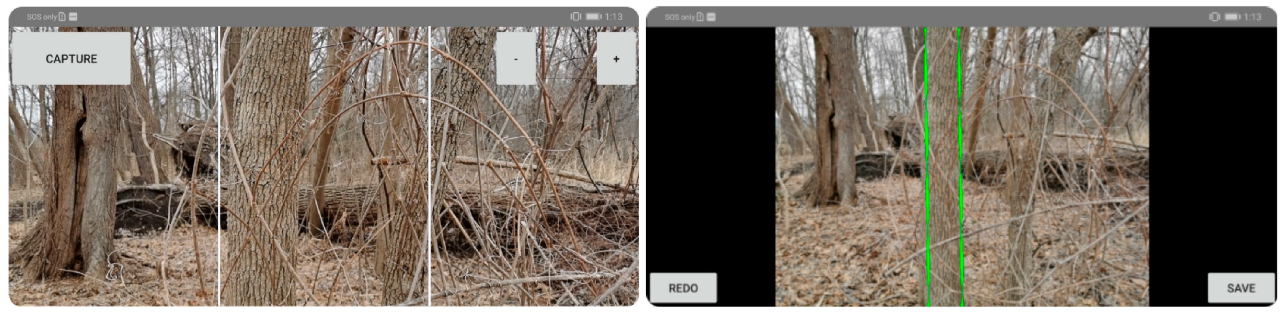
2.2. App Design and User Experience

In this work, we design an app for an Android phone with a depth sensor. The app allows users to walk around a forest, taking pictures of each tree as they pass it. The main app screen is a continuously updated color camera preview, similar to one that users may be accustomed to in a standard camera app (Figure 1 left). The preview screen has a “Capture“ button and two lines overlaid on the image dividing it into thirds, guiding users to center the tree in the image. When the user points the phone at a tree trunk and selects “Capture,” the app saves the color (RGB) and depth frames from the camera sensor and initiates the processing algorithm. This does not require an internet or cell connection; the algorithm is run locally on the phone.
We designed our system for speed, both in terms of user input time and computational time. Thus, the user only needs to take one picture of the tree from 1–2 m away. They do not need to capture the tree from multiple angles and can stand in whichever spot near the tree is most accessible, according to understory conditions. The algorithm itself completes in under a second, allowing two-way communication between the user and the app. When the algorithm completes, the estimated trunk boundaries are reprojected onto the RGB image and immediately displayed back to the user (Figure 1 right). The user can then assist the app with a one-click confirmation, selecting “Save” or “Redo” based on whether the algorithm appears to have successfully identified the trunk. This confirmation step is intended to be a quick check to eliminate cases where the algorithm is widely off or incorrectly identifies another object in the frame as the tree; the user is not expected to carefully judge the accuracy of the diameter estimate. The fact that the image processing takes place locally in near-real time also allows the app to assist the user, displaying algorithm errors and directing the user to adjust their position if necessary. We further discuss the effects of this confirmation step on the tree detection rate in Section 3.1.

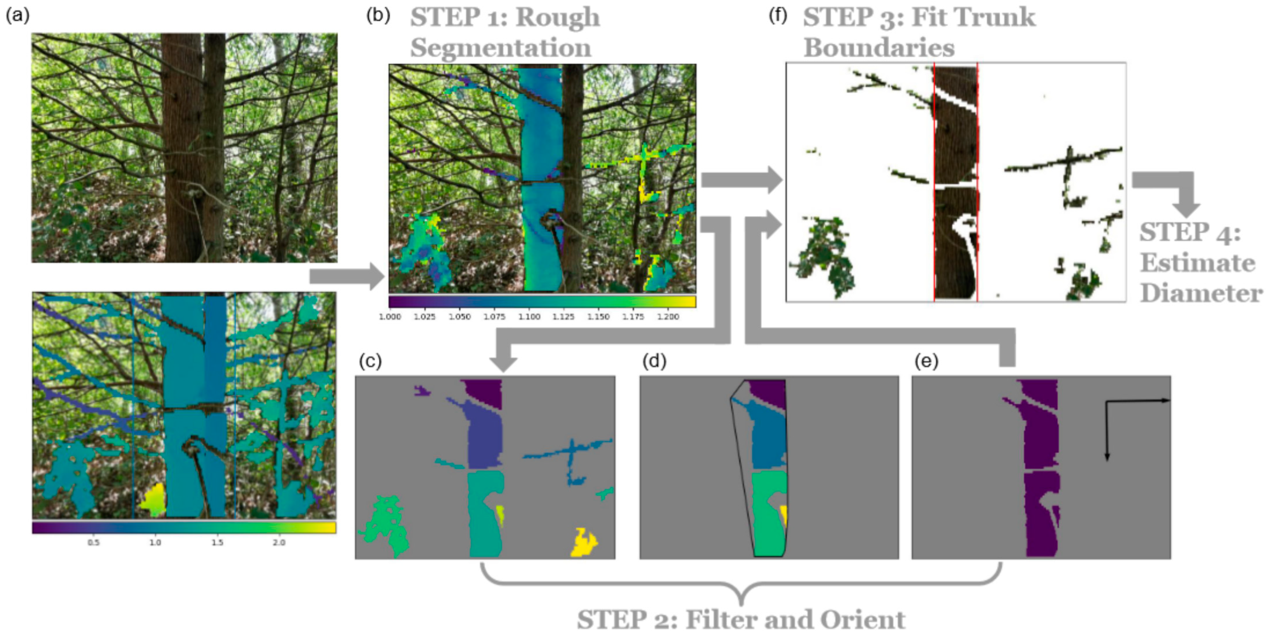
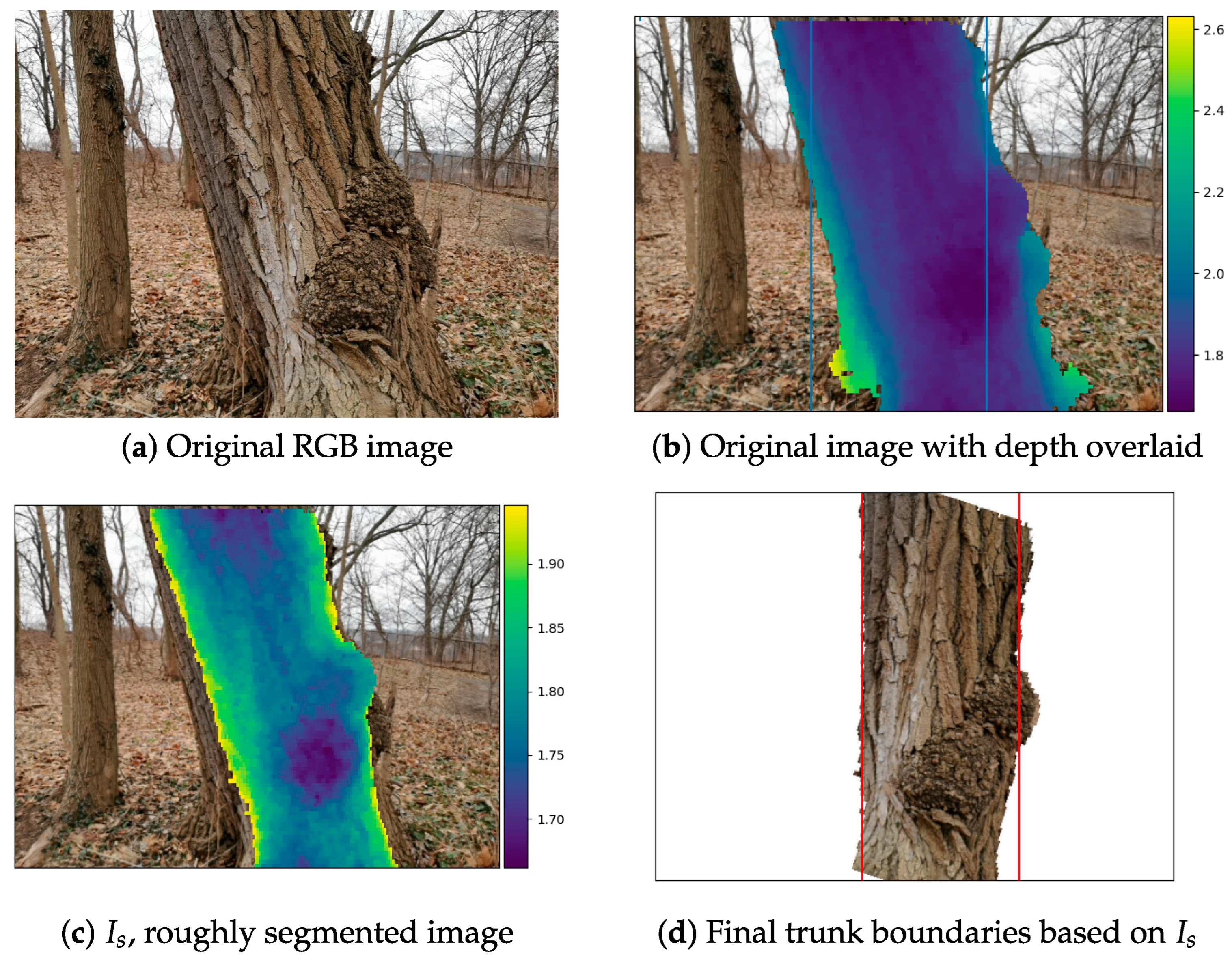
2.3. Image Processing Algorithm

In the following sections, we present our core image processing algorithm for identifying trunks and estimating their diameters, which is automatically invoked when the user taps the app’s “Capture“ button. In Figure 2, we demonstrate each step of the algorithm on a sample tree image with considerable occlusion (the original RGB and depth images are shown in Figure 2a).

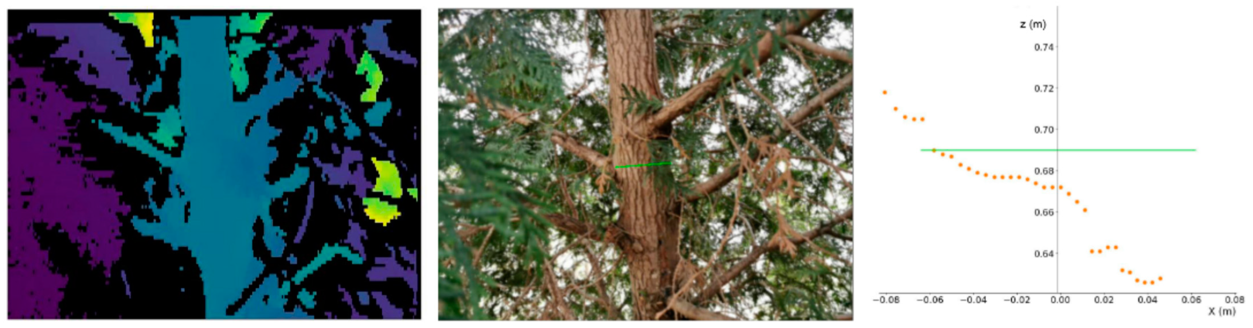
2.3.1. Step 1: Approximate Trunk Depth

To begin, we make a rough estimate of the trunk depth, which guides the subsequent processing. We expect the trunk to contain a large set of points of similar depth (unlike vegetation or branches, which will either be of relatively inconsistent depth or small size). We make the natural assumption that the user will attempt to center the tree trunk in the image, and we also provide guiding lines in the app to help the user do so. To estimate trunk depth, we slice the image vertically into thirds, bucket the depth values in the center third of the image into 3 cm ranges, and take the mode bucket as the approximate trunk depth δ m . We then filter the image for pixels whose depth value is within ± 10 % of δ m . This forms a rough segmentation, or labeling of the image pixels, I s .

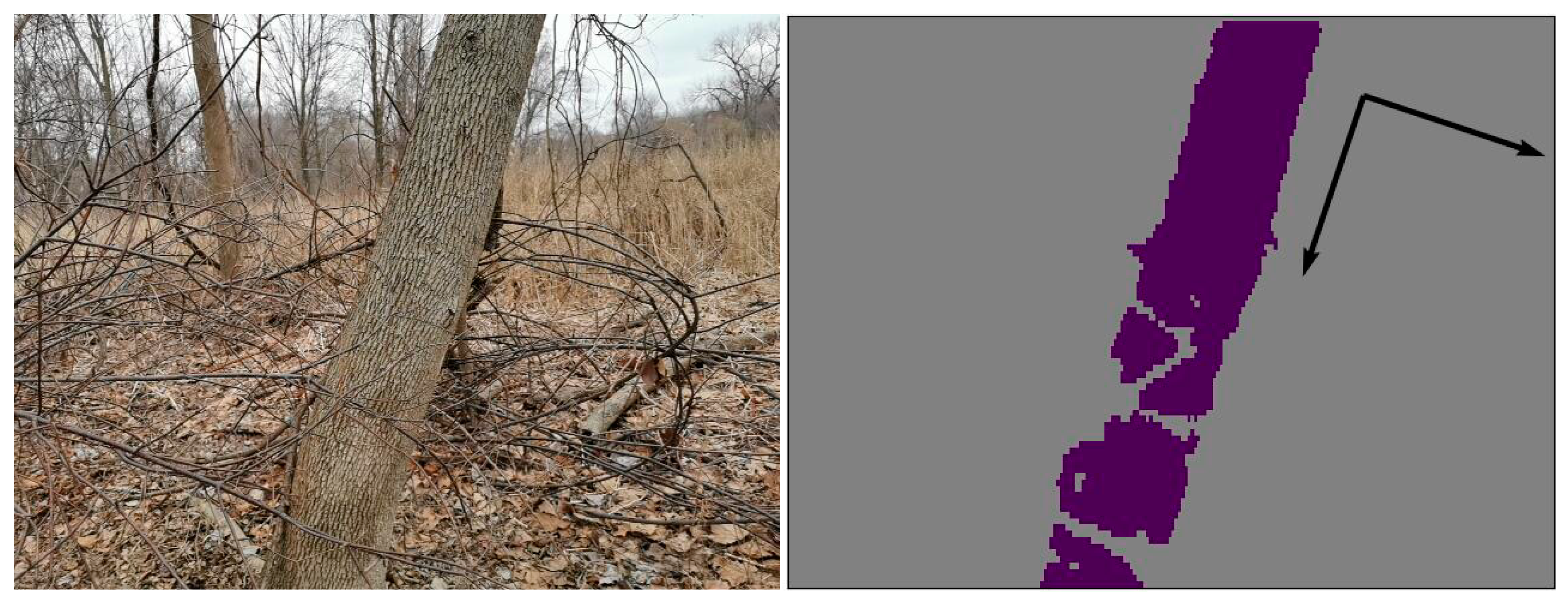
2.3.2. Step 2: Filter & Orient Trunk Pixels

I s ’ may include some leaves and branches that happen to match the trunk depth while omitting portions of the trunk that are obscured by closer leaves and branches, as seen in image (b) of Figure 2. Conceptually, we now want to find a tight boundary for the trunk that will exclude these outliers while still containing (“filling in”) the obscured portions. The distance between the left and right sides of this boundary will then correspond to the diameter of the trunk. We also require the orientation of the trunk, because the diameter must be estimated perpendicular to this orientation. Finding the orientation first improves the efficiency of boundary detection: we use the orientation angle to rotate the image so that the trunk is vertical and search only along vertical lines for appropriate trunk boundaries.
Overall, the pixels in I s are typically dominated by trunk pixels, which form a rough oblong cluster. We follow the approach described by Rehman et al. [18] for automatically aligning such images, finding the principal axis of the trunk using principal component analysis (PCA). PCA is sensitive to outliers but is able to identify the principal axis relatively well even with a small subset of the trunk pixels missing. As a result, we prefer to over-filter the image, ensuring that few non-trunk pixels remain, even at the possible cost of losing some true trunk pixels. We call this highly filtered input to PCA I f . (Notably, I f will not be suitable for identifying the boundaries of the trunk directly. The over-filtering at this stage would lead to underestimating the trunk diameter.)
To obtain I f , we remove two main sets of outlier pixels: small clusters of pixels corresponding to individual leaves or small elements in the environment and substantial objects (e.g., shrubs, large branches, additional trunks) that happen to share the trunk depth. We begin by parsing I s into its connected components [19], an example of which can be seen in image (c) of Figure 2. To filter out small clusters, we remove all connected components below a threshold number of pixels, α = 300 pixels. This thresholding is analogous to the pre-PCA filtering performed by Rehman et al. [18].
Depending on the level of occlusion, the trunk may be split across multiple connected components, as is the case in image (c) of Figure 2. We need to identify which subset of components comprise the trunk and which correspond to other objects in the image. Since the underlying trunk is a large, oblong shape, the set of connected components that represent the trunk should, intuitively, form a dense cluster in the image. Here, we define the density of a set of connected components as the ratio of the area of the components to the area of the convex hull around those components. Large components that represent leaves and branches will tend to extend beyond the convex hull around the trunk components, because they are far from the main trunk or point in a different direction, so including them in the trunk subset will result in a low-density measurement. Our algorithm, therefore, searches for a dense subset of components in the image (Appendix A.2); this subset is I f .
I f is a highly filtered version of the image; we show a sample I f in image (d) of Figure 2, with the fitted convex hull outlined in black. To perform PCA, we use the set of pixel coordinates where I f is non-zero. PCA computes the eigenvectors of the covariance matrix of these data points, which indicate the direction of maximum data spread. Based on these eigenvectors, we can identify the principal axis of the trunk and orient the image so that the trunk is vertical, as shown in image (e) of Figure 2. Rotating the image using PCA was robust even with highly tilted trunks (see, e.g., Figure A1 in Appendix A.3).

2.3.3. Step 3: Identify Trunk Boundaries

With the principal axis identified, we return to I s (Figure 2b), the minimally filtered image, to search for the trunk boundaries. We use the direction of the principal axis found in Step 2 to rotate I s to orient the trunk vertically. We then use a two-pass algorithm to iterate through vertical scan lines of a binary version of I s , which is 0 where I s = 0 , and 1 otherwise. We first iterate inward until reaching a line at which the ratio of nonzero pixels to zero pixels exceeds a high threshold, T h i g h = 0.6 , then back outwards until the ratio of nonzero pixels to zero pixels falls below a low threshold T l o w = 0.5 . The final segmentation consists of all the pixels in I s that lie within this boundary, as shown in image (f) of Figure 2. To select T h i g h and T l o w , we vary these parameters over a small test data set of trees collected from a Carolinian forest in leaf-on conditions (the Laurel Creek location described in Section 2.4.2) and choose the thresholds that result in the lowest bias (mean error) metric. It is possible that accuracy could be improved by setting these parameters based on a test sample specific to each study area, but we use the same parameters in all evaluation environments.

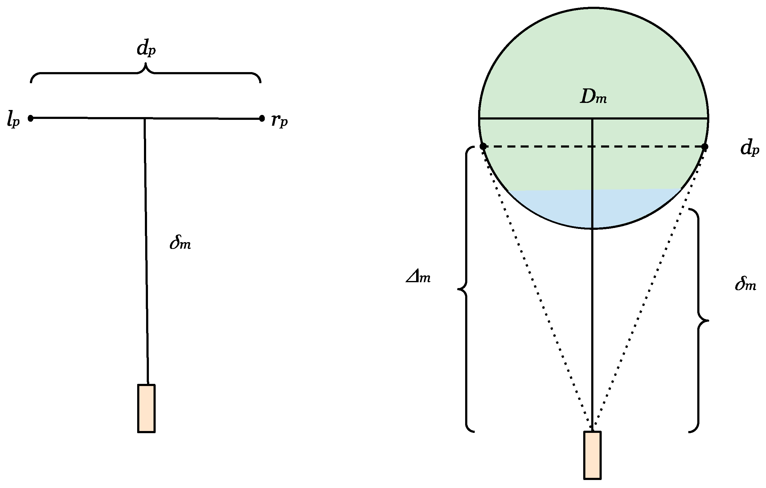
2.3.4. Step 4: Estimate Diameter

Finally, we translate the trunk boundaries and depth pixel values into a diameter estimate. In the equations below, we will use the subscript p to denote a quantity in pixels, and m to denote a quantity in meters.
In general, distances in an image are related to real-world distances by the sensor’s calibration constant, γ p , which is defined as the width, in pixels, of a 1 m object at a depth of 1 m. The length of an object k meters away that appears to be d pixels wide in an image is   
d m = d p · k m γ p
We can, thus, obtain a first approximation of the diameter of the tree as follows: the left and right boundary lines found in Step 3 (Section 2.3.3) can be defined as the lines x = l p and x = r p , respectively. We set d p = l p r p and k m = δ m in the above formula, where δ m is the modal depth in the center third of the image.
However, the simple approximation given in Equation (1) tends to consistently underestimate the trunk diameter, especially for large trees and when the user stands close to the trunk. This is because this equation does not account for the geometry of the trunk, which forms a rough cylinder that extends closer to the sensor than the true depths of the left and right boundary lines. It also does not account for parallax effects: the sensor will not capture pixels at the widest part of the trunk (on the true diameter, if the trunk were a perfect cylinder). Rather, the boundary pixels will occur on lines tangent to the trunk perimeter that intersects with the depth sensor location, and so will define a smaller chord than the diameter.
The derivation shown in Appendix A.4 accounts for the effects of parallax and the tree geometry to arrive instead at the following diameter estimate, D m :
D m = d p · δ m γ p d p 4

2.4. App Evaluation

2.4.1. Mobile Phone Hardware

We evaluated our app on a Huawei P30 Pro phone, which, at the time of purchase, retailed for around USD 1100, but has since fallen to under USD 600. The P30 has three rear-facing cameras (40, 20, and 8 MP), one rear-facing time-of-flight (LiDAR) sensor, and a front-facing camera (32 MP). It is also equipped with 128 GB of SSD storage, 6 GB of RAM, an 8-core CPU, and a separate GPU. Huawei does not publicly disclose the full specifications of its LiDAR sensor, though investigative teardowns of the phone reveal that the sensor uses the Lumentum flood illuminator to emit infrared light, and Sony’s integrated circuit image sensor [20,21]. The sensor has a resolution of 180 × 240 pixels.

2.4.2. Measurement Environment and Procedure

We evaluated our work in three different forest areas, which are summarized in Table 1. Sample images from each evaluation plot can be found in Appendix A.6 and all RGB and depth images used in the evaluation are available at http://dx.doi.org/10.5061/dryad.vdncjsxxj (accessed on 27 January 2023). The Laurel Creek forest is a naturally managed Carolinian forest [22] with a mixture of broadleaf and conifer species. Midsummer leaf-on conditions resulted in significant trunk occlusion from leaves and branches across the samples. The topography of the preserve is relatively flat, with elevation gains of up to 30 m [23]. The Beechwoods Nature Reserve is dominated by beech trees, the oldest of which were planted in the 1840s. It also contains moderate understory growth of English yew, hemlock, and holly [24], but it is possible to walk through largely unobstructed. It has little to no elevation change. The Van Cortlandt Park Preserve includes old-growth forests and some wetlands, with a diverse array of black oak, sweetgum, red maple, and other, mostly deciduous, species native to the northeastern United States. At the time of our evaluation, it was under active ecological restoration to remove non-native invasive, such as oriental bittersweet (Celastrus orbiculatus), a vine that strangles native trees, and Rosa multiflora, a shrub whose thickets smother competing plant growth [25]. Even in winter leaf-off conditions, the climbing vines and underbrush led to significant trunk occlusion and difficult walking conditions in many areas. It contained up to 50 m of elevation gain and rocky terrain [26].
At the time of the Laurel Creek evaluation, users could not retry samples and were not able to view the captured images or see the results of the algorithm until they had left the forest. The Laurel Creek data, thus, included 2 samples each of 14 trees, with 1 set taken at 1 m and the other at 2 m away. In the Beechwoods and Van Cortlandt sites, the app provided displayed the results back to the user, as shown in the bottom panel of Figure 1. The Beechwoods data included 87 images of 42 trees, and the Van Cortlandt sample included 53 images of 29 trees. There were more images per tree when the first images were rejected by the user based on the on-screen presentation of results and errors. The user was instructed to stand roughly 1.5 m from the tree, at a comfortable distance according to site conditions. The resulting images included trunks that were 1 to 2 m away. In all samples, we established ground truth by measuring the circumference of each tree with a tape measure and computing the reference DBH to the nearest tenth of a centimeter. Abnormally shaped trunks with burls or other irregularities at breast height were measured according to the standards outlined by Schlegel et al. [6].

3. Results

3.1. Trunk Detection
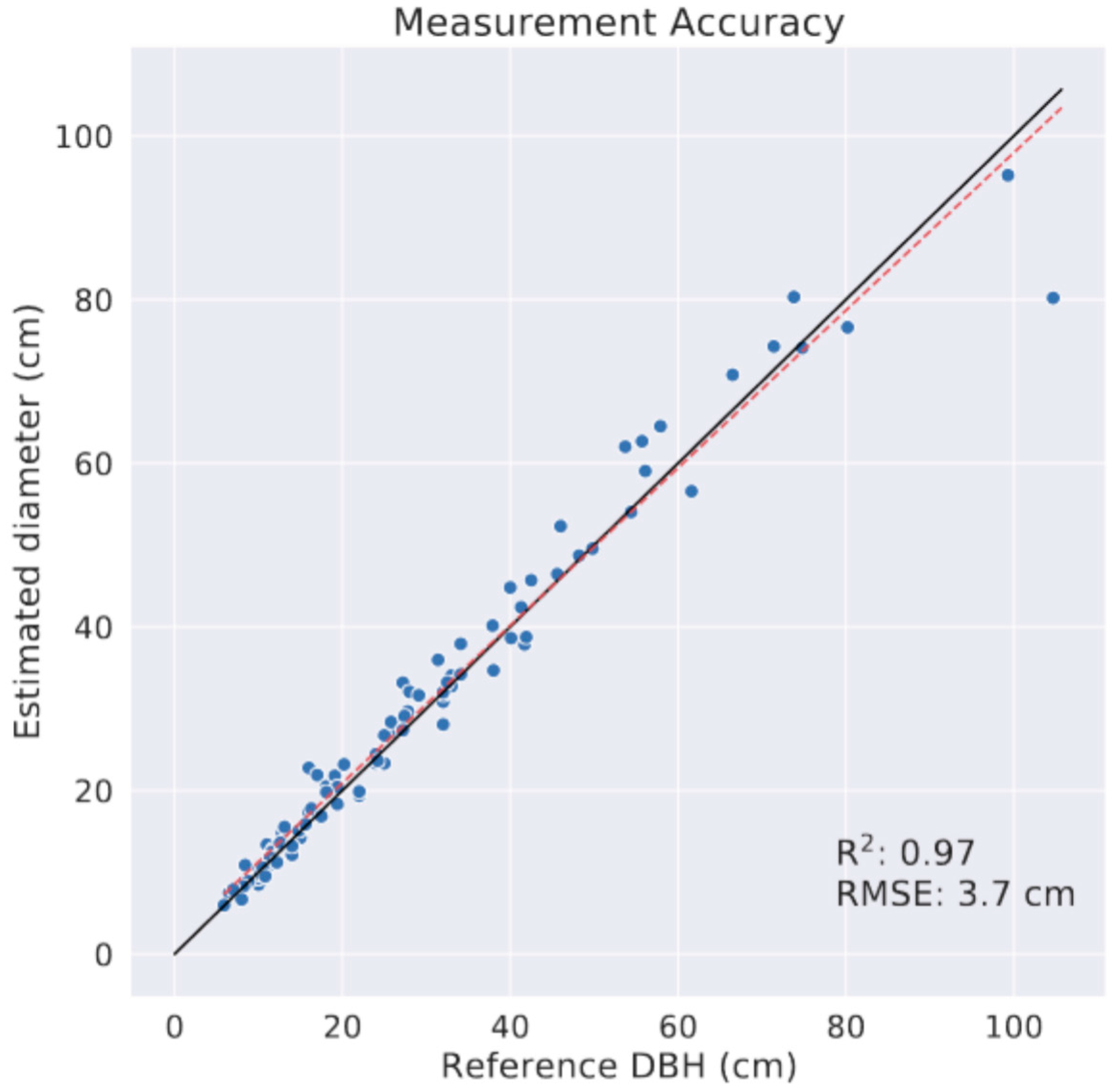
In the Laurel Creek data set, collected when the app had a limited user interface that did not offer any user assistance (users could not even view the image they had just captured), the tree detection rate was 93%. In one of the images, the camera was unable to obtain any depth points. A later version of the app would have identified this as an error and relayed it to the user. In another sample, some of the depth points were captured, but they did not correspond to the tree trunk. This would have been identified as a warning in the later version of the app.
With the version of the app interface used in the Beechwoods and Van Cortlandt evaluations, which included warnings and an on-screen presentation of results, the system achieved a 100% detection rate. By examining these two data sets further, we can compare the effect of user assistance between multiple image captures of the same tree. Note that we require the user to save the first image they capture, whether or not warnings were displayed or they believed the app failed to capture the trunk. In Figure 3, we compare the results for each tree measurement between the first captured image and the last, “best attempt“ image, which the user believed based on app feedback had successfully captured the trunk. In 29 of 71 trees (41%), the first image was considered a satisfactory measurement—in these cases, the first and last captured images are the same. 79% of trees were captured satisfactorily in at most two images, and 96% in at most three. In cases when more than one image was required, it was usually a quick adjustment to avoid a leaf or branch in the way of the trunk. In the unassisted set of first images, 5 images had well over 20 cm in errors because no trunk was found or an incorrect object was identified as the trunk, with a 93% detection rate. In the assisted set of last images, the tree trunk was found in all images. Incorporating user assistance in the app interface, thus, allowed us to improve trunk detection overall.

3.2. Accuracy

For the following section, we report the accuracy of results only for images in which the tree was detected. For the Beechwoods and Van Cortlandt data sets that incorporated user assistance, this means that we consider only the last, “best attempt” image for each tree. Our results are therefore reported on 26 images in the Laurel creek data set and 42 and 29 images for the Beechwoods and Van Cortlandt data sets, respectively.
We find that the app’s diameter estimates are in good agreement with measured DBH ( R 2 = 0.97), as shown in Figure 4. Overall, the RMSE was 3.7 cm, with a bias value (mean error) of 0.6 cm. The mean absolute percent error was 8.0%. The RMSE was affected by an outlier in the Van Cortlandt data set: a 1.04 m diameter tree with −24 cm of error (23%). We discuss the cause of this outlier and ways to correct it in Section 5. If we omit this sample in the combined data set (including only trees with diameters under 1.0 m), the overall RMSE drops to 2.7 cm, with a bias of 0.9 cm and a mean absolute percent error of 7.8%. We show more detailed numerical results in Table 2. These errors are higher than TLS, which consistently achieves 1–3 cm RMSE even in complex forest plots [27]. They are more in line with both the 1.2–5.1 cm error range reported in prior work with mobile devices [10,11,12,13,16,28] and with estimates of a 3–7% coefficient of variation in manual DBH measurements or up to 12.8 % with untrained surveyors [29]. Table A1 in Appendix A.5 provides a systematic comparison with prior work.

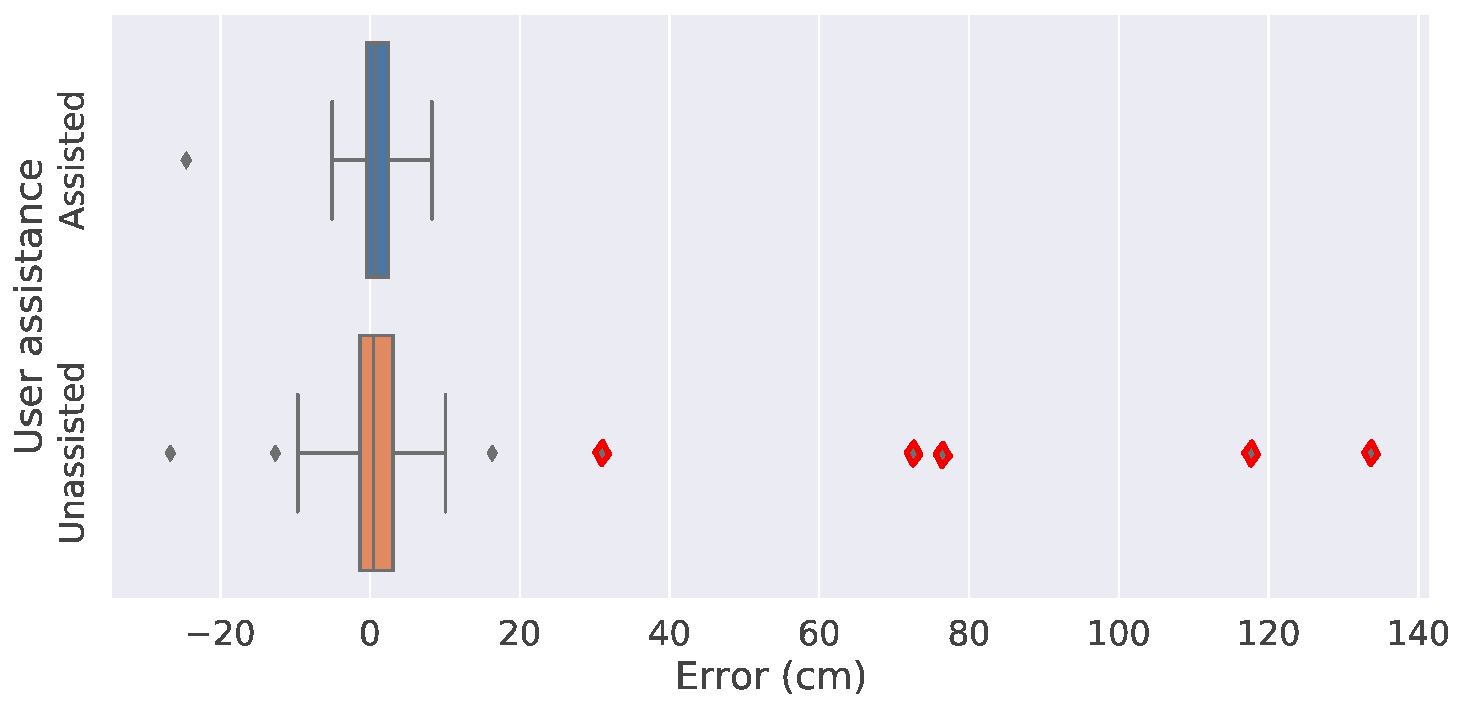
3.3. Data Collection Time and Ease of Use

One key strength of our designed system is the speedup in measuring trees in the field. In a survey in Van Cortlandt Forest, we timed the manual and app-based measurement of trees in sets of two to three nearby trees at once, and found that the app reduced surveyor time by up to a factor of 4.6, with a mean speedup of 3.6×. Some of the time saved was by avoiding walking through the underbrush from one tree to the next since the user could traverse less distance and stand in more convenient locations when using the app.
One particular sample highlighted the ease and efficiency of our system: measuring a small stand of northern white cedars (Thuja occidentalis) in the Van Cortlandt Forest. The cedars are depicted in Figure 5. The trunks are impossible to see or reach directly from the exterior of their canopies, meaning that in order to measure their circumference manually, the surveyor had to find an appropriate gap in the branches and crawl underneath. By contrast, with the designed app, they could simply hold the phone just inside the outer canopy and measure the trunk within. The measurement of the two cedars took around 2.5 min manually and less than 30 s with the app.

4. Discussion

Our algorithm does not attempt to explicitly estimate DBH by, for example, identifying the ground plane, determining the cross-section of the trunk 1.3 m above this ground level, and fitting a circle to the depth points at this location. Instead, we develop a diameter estimator, which allows us to produce a robust estimation from a single mobile LiDAR depth image with minimal manual intervention. With the low-end LiDAR sensors offered on mobile devices, the common approach of fitting a circle to the depth points at a cross-section of the trunk [10,13] is not reliable for images with high occlusion. For example, in Figure 6 we show the depth and RGB images captured by our app for the tree shown in Figure 5. The images were taken with the phone held just under the tree canopy. Based on these images, our app was able to estimate the diameter of the tree with <1 cm of error. However, the cross-section of depth points on the trunk, shown on the right in Figure 6, does not look circular, because of the branch on the left side sloping away from the camera and the branch and needles on the right sloping toward it. Obtaining an accurate diameter estimate by fitting a circle to the points in this cross-section would not be straightforward. It would also have been challenging to walk around this tree while maintaining line-of-sight contact between the phone LiDAR sensor and the trunk, given the tree’s thick needle canopy and dense branching.
In our work, we take a “whole bole” approach to estimate the trunk diameter, similar to cylinder-fitting methods used for TLS data [30,31], by following the assumptions of DBH measurement in a way that is more natural for image data. For example, DBH is not always measured at 1.3 m above ground level: if a branch or large burl occurs at this height, surveyors must measure at another height, where the branch or burl no longer affects the results [6]. DBH measurements also implicitly model the tree as a cylinder by measuring the trunk’s circumference and dividing by π . Our technique is similarly robust to branches and burls, modeling the trunk of the tree without these irregularities. To achieve this robustness, we use as input the entire range of the trunk visible in the image and estimate the edges of the trunk based on a threshold majority of pixels throughout that range. Fitting linear boundaries and estimating the trunk according to Equation (2) use the same modeling assumptions of the cylindrical shape of the trunk as manual DBH measurement. Finally, we evaluate our diameter estimates against the DBH measured manually using traditional forest inventory methods and find that it has small errors and biases relative to these measurements.
However, our approach is not without its limitations. We evaluated our system on a diverse range of tree sizes, from 6 to 104 cm in diameter, a wider range than any previous work we are aware of using mobile phone depth sensors. In its current iteration, though, our algorithm may give poor results on trees outside of the evaluated range. The largest tree measured in our data set was a 1.04 m diameter tree in Van Cortlandt forest, and it was a significant outlier in terms of estimation error, with a final diameter estimate that was off by 24 cm (23%). A close analysis of the algorithm’s performance, in this case, reveals that the fault lay in the first step of the algorithm. Part of the tree was omitted when filtering for depths within ± 10 % of the mode trunk depth due to the shape and size of the trunk, which affected both the rotation of the image and the estimation of trunk boundaries Figure A6 in Appendix A.7). There were other trees in our evaluation data set of similar size (the second-largest tree had a 99 cm DBH) that did not have similar problems. However, we note that only 13% of our evaluation data set has a DBH over 50 cm, and further evaluation is required to assess the algorithm’s accuracy on large trees. Moreover, to consistently handle large and irregularly shaped trunks, such as the one discussed here, a more flexible first step of the algorithm may be required. For example, we might consider incorporating the RGB image into the initial rough segmentation, which we did not otherwise find necessary. Alternatively, we could search for edges (pixels dissimilar to their neighbors) in the depth image, rather than depths within a particular range. In addition to adjustments for large trees, there are other forested areas, particularly in the tropics, which present further challenges for mobile phone LiDAR systems such as ours. For example, while our app handles the occlusion from leaves, branches, and low-lying vegetation found in our tested environments, it does not handle lianas or buttressed trees, and has not been tested with the diversity of tree sizes and forms found in the tropics. Handling an even broader range of trees and forest conditions is a highly appropriate direction for future work.
In the existing literature on using short-range, low-end sensors for estimating a diameter, algorithm robustness, especially regarding the occlusions that naturally occur in diverse forest environments, is under-studied. The literature that performs evaluations in such environments uses manual segmentation of depth points [11] or computationally intensive algorithms that must be run offline on a desktop computer [15,16]. We contribute to the research in this area by highlighting the challenges that low-end mobile depth scanners face in occluded conditions and offering a lightweight, fully automatic approach for segmenting depth images and estimating trunk diameter despite these challenges.

5. Conclusions

We demonstrate the use of smartphones equipped with depth sensors to estimate the trunk diameters of trees in forest plots. In many forest environments, trunk images can be occluded, lighting conditions can be challenging, and it may not be easy to walk around each tree. Unlike previous research into using mobile phones, our work considers the presence of undergrowth and occlusion as a primary use case. We design an algorithm that requires only a single image to estimate diameter and is computationally efficient enough to run directly on a mobile phone in near real-time. We incorporate our algorithm into an interactive mobile phone app with user feedback and evaluate our system in partly-managed forest settings. We find that in a corpus of 97 sample tree images, it estimates trunk diameters with a RMSE of 3.7 cm ( R 2 = 0.97; 8.0% mean absolute error). This is comparable to the results achieved by prior approaches but, unlike prior work, our solution is capable of obtaining results in a dense, leafy understory. We believe that our proposed system is a promising direction for research in the use of sophisticated smartphone technologies for performing robust, efficient, and inexpensive in situ forest carbon estimates.

Author Contributions

S.K., L.T. and A.H. conceived the idea and design methodology; L.T. and A.H. implemented the mobile phone application and image processing algorithm; A.H. collected and analyzed the data and led the writing of the manuscript. S.K., L.T. and A.H. contributed critically to the drafts and gave final approval for publication. All authors have read and agreed to the published version of the manuscript.

Funding

The authors received support from the David Cheriton Graduate Scholarship, the Canadian National Research Council, and the Harding Distinguished Postgraduate Scholarship.

Institutional Review Board Statement

Not applicable.

Data Availability Statement

The algorithm and app code are publicly available on GitHub at https://github.com/ameliaholcomb/trees/tree/master/trees (accessed on 27 January 2023). Data available from the Dryad Digital Repository http://dx.doi.org/10.5061/dryad.vdncjsxxj (accessed on 27 January 2023).

Acknowledgments

The authors thank Connor Tannahill for his help when this research was in its earliest stages, and Sarab Sethi for his feedback and mentorship during the writing process.

Conflicts of Interest

The authors declare no conflict of interest.

Appendix A

Appendix A.1. Algorithm Assumptions

This supplement discusses the assumptions made in the design of our algorithm, some of which may be limitations on the environments in which our system can be used.
  • The tree is within ± 45 degrees of vertical: PCA yields two perpendicular eigenvectors, whose orders are not guaranteed to be related to the true principal axis of the trunk. We, therefore, assume that the correct eigenvector is within 45 degrees of the vertical. This assumption seems reasonable for most trees.
  • The tree does not lean steeply toward or away from the camera: If the tree is leaning toward or away from the camera, rather than on a plane perpendicular to it, we will not be able to successfully find the orientation of the tree. This will affect the angle of the diameter line and may cause errors in fitting a vertical boundary to the trunk. Moreover, we will filter out too many of the true trunk points in the 10% filter. Although it is not straightforward to detect that an image has this problem, we can instruct the user to take pictures (in which this is not the case). It may be interesting to observe that we realized this limitation only after the evaluation data sets were collected, and none of the images had this problem. It may be somewhat unnatural to stand under or over a steep leaning tree in order to take a picture of it, though user studies would be required to confirm this.
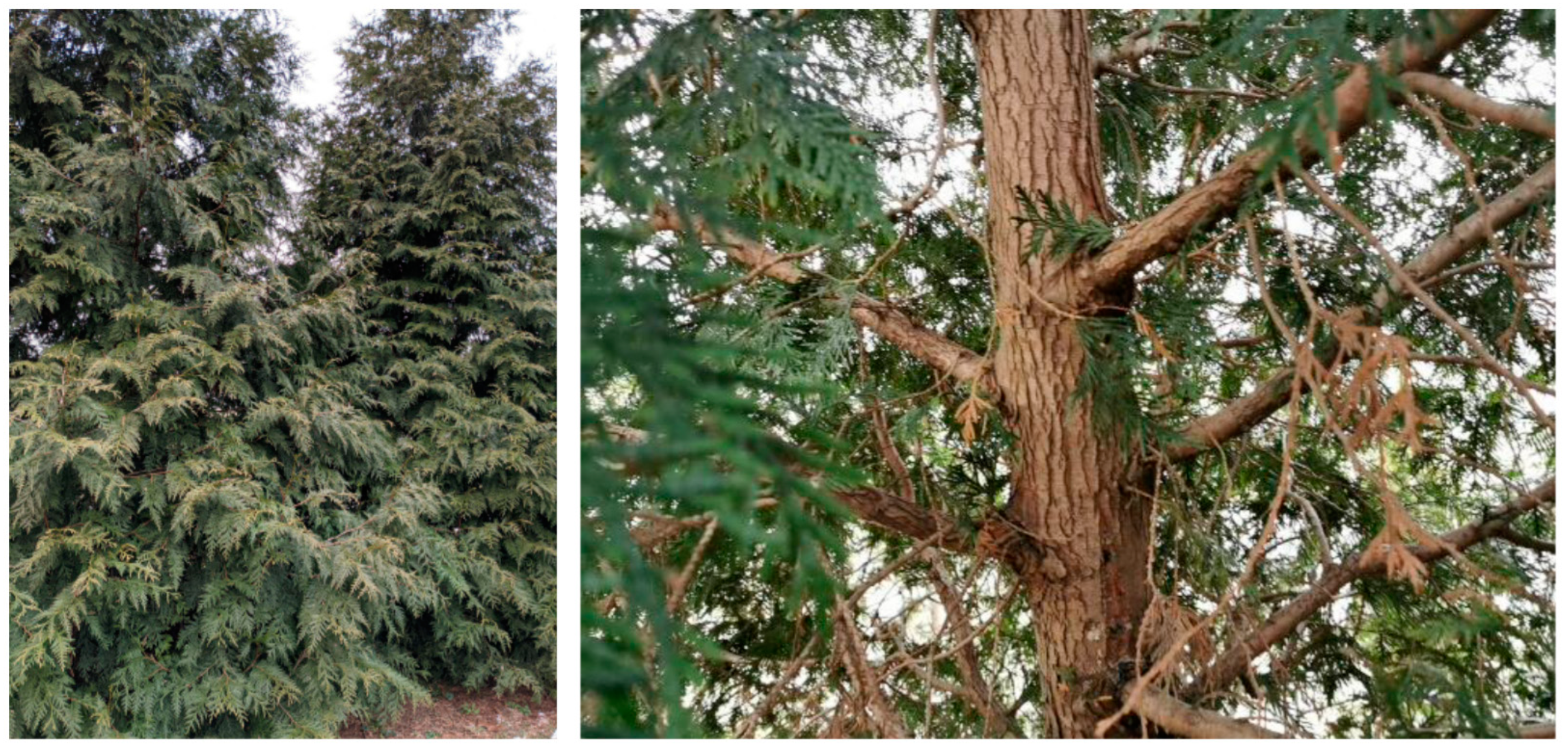
  • The trunk is roughly cylindrical: We assume that the trunk is roughly cylindrical when fitting boundaries to it and estimating the DBH, although we can handle some amount of irregularity, such as the large burls found on some of our evaluation samples. The IPCC standard manual measurement techniques [6] also make this assumption. However, we believe that the ideal system should not rely heavily on this assumption, and we believe that future work should consider handling such trees.
  • The tree has one trunk: We only estimate the diameter for one trunk per image. It would be primarily a UI change to allow multiple trunks for a single tree sample, giving the user an option to “add a trunk to this sample“ after saving the image of the first trunk.
  • The tree is small enough to fit within the camera frame at 2–3 m away: At 2 m away, the camera frame can capture a trunk of roughly 2.7 m in diameter. This is nearly three times the maximum tree diameter that we were able to test on. If larger trunks are required, some of the same approaches used to address non-cylindrical trunks could also be used in this context.

Appendix A.2. Filtering Algorithm

This supplement describes in more detail the algorithm used to find a dense subset of connected components in the partly filtered image, I s , in order to arrive at I f . We search for this dense subset by removing components one by one in the order of the distance of the horizontal center of mass from the horizontal center of mass of the largest non-background component in I s , which is assumed to be part of the trunk. Specifically, the horizontal center of mass, m i , of a set of pixels, i, is the mean x-coordinate of those pixels. We then sort the components by m i m t , where t is the largest component in I s . We stop removing components once the image contains only a set of components above a threshold density. We found through empirical trials that a threshold value of β = 0.60 works well.
The pseudocode for this Algorithm A1 is as follows:
Algorithm A1: Algorithm pseudocode to find dense subset of connected components.
Remotesensing 15 00772 i001

Appendix A.3. Identifying the Principal Axis of a Tilted Trunk

Figure A1. The eigenvectors found by PCA can be used to robustly identify the principal axis of a highly tilted trunk. (Left) RGB image. (Right) Binary version of I s , with eigenvectors overlaid as black arrows.
Remotesensing 15 00772 g0a1

Appendix A.4. Diameter Estimation

This supplement gives the explanation and derivation of Equation (2). The intuition behind the simple approximation of the diameter given in Equation (1) is shown on the left side of Figure A2. The derivation below accounts for the effects of the parallax and the geometry of the trunk, based on the intuition shown on the right side of Figure A2.
The boundary lines found in Section 2.3.2 provide a relatively robust understanding of the width of the tree because we estimate them based on the entire visible length of the tree, and because they do not rely heavily on the precise depth values at the edge of the tree—only that the values are non-zero. Figure A2 shows that small changes in the location of the tangent points l and r have a small effect on d p , as long as the tangent points are roughly near the true diameter line of the trunk. (The width of a circle changes most slowly near its diameter.) We make the simplification that d m , the distance in meters corresponding to d p , is roughly equal to D m , the true diameter.
By contrast, changes in δ m will have a linear effect on our estimated diameter (as the simple approximation in Equation (1) shows). Therefore, we cannot make the approximation that δ m , the mode trunk depth, equals Δ m , the depth at which the boundary lines are estimated. Instead, we estimate Δ m as a correction to our measured depth δ m by adding some fraction, 1 c , of the (unknown) true diameter of the tree.
Δ m = δ m + D m c
where 0 < 1 c < 1 2 . D m c can be at most the radius of the tree, D m 2 : in this case, δ m was measured at the closest point on the tree to the sensor, and the ToF sensor was infinitely far from the trunk so that d p was an image of the true diameter of the tree.
Then we rewrite Equation (1) in terms of Δ m , with the approximation discussed above that d m = D m :
D m = d p · Δ m γ 1 p
Solving these two equations for D m , the diameter of the tree, we obtain
D m = d p · δ m γ 1 p d p c
Based on the analysis of sample tree cross-sections, we found that in more regularly shaped trunks our estimated depth δ m tends to lie around halfway between the front of the tree and the approximate depth of the boundary lines. This leads us to set 1 c = 1 4 , halfway through the possible range of c.
Figure A2. Diagram showing different methods of the approximate tree diameter. Left: Bird’s-eye-view diagram representing a simple approximation of the ToF sensor (colored orange) pointed at a tree. The left and right boundary lines determined in Section 2.3.2 are pointing straight up out of the page at the points labeled l p and r p . We can approximate the tree diameter in pixels, d p , as the number of pixels between them. In this simple approximation, we assume that the diameter line is at a distance δ m from the sensor, where δ m is the approximate trunk depth calculated in Section 2.3.1. Right: Modified bird’s-eye-view diagram of the ToF sensor pointing at a trunk. Since the tree is three-dimensional and roughly cylindrical, the left and right boundary lines found in Section 2.3.2 lie on a cylinder (shown here as a circle) around the trunk. d p , the distance between the left and right boundaries, is not the diameter of this cylinder, D m , but rather the length of a chord slightly closer to the ToF sensor than the true diameter. This is because of the field of view of the ToF sensor (represented by dotted lines). δ m , the approximate depth of the trunk found using the mode depth in the center third of the image (Section 2.3.1), does not correspond to Δ m , the depth of the chord d p , but instead to a smaller depth somewhere in the blue region at the front of the cylinder.
Remotesensing 15 00772 g0a2
It is worth discussing the major concern with this equation, namely: what happens when γ 1 p d p c 0 . If γ 1 p = d p c , consider what it means for the physical system. γ 1 is the number of pixels of a 1.0 m object at one meter away. When γ 1 p = d p c , this means some fraction 1 c of the observed trunk diameter appears indistinguishable from a 1.0 m wide object viewed by a ToF sensor 1.0 m away. In other words, the full trunk diameter would look similar to a c-meter-wide object at a distance of 1.0 m. Even taking c to be as small as possible ( c = 2 ), this gives us a trunk diameter of 2.0 m viewed from a distance of 1.0 m, which is to say, the picture we have is indistinguishable from that taken by a ToF sensor placed directly on the trunk.

Appendix A.5. Comparison with Prior Work

Table A1. Comparison with prior work.
ReferenceTechnologySingle Image per TreeOn-Device ProcessingHandles OcclusionsManual InterventionEvaluated DBH RangeReported DBH RMSE
This studyHuawei P30 ProYesYesYesOptional (retake image)6–104 cm * 3.7 cm; 2.7 cm for trunks up to 100 cm.
Tatsumi et al. [13]iPhone 13 Pro/iPad ProNoYesNoYes (measure 1.3 m height)5–70 cm2.27 cm (iPhone)/
2.32 cm (iPad)
Çakir et al. [11]iPad ProNoNoYesYes (remove occlusions)31.5–59.7 cm2.9 cm (Urban forest)/2.5 cm (Managed forest)
Gollob et al. [15]iPad ProNoNoYesNo5–59.9 cm3.64 (3D Scanner)/4.51 (Polycam)/3.13 (SiteScape)
Hyyppä et al. [32]Google Tango/ Microsoft KinectNoNoUnknownYes (image segmentation)6.8–50.8 cm0.73 cm (Tango)/1.9 cm (Kinect)
Mokroš et al. [12]iPad Pro/ MultiCam PhotogrammetryNoNoUnknownNo3.1–74.3 cm2.6–3.4 cm (iPad)/6.98 cm (MultiCam)
Fan et al. [10]Google TangoYesYesNoNo6.1–34.5 cm1.26 cm
Piermattei et al. [16]Nikon cameraNoNoYesNo6.4–63.9 cm1.21–5.07 cm
KATAM [17]Most mobile phones supportedContinuous videoOn-device but not real-timeNoNoN/AUnknown
* Limited evaluation of trees with DBH over 50 cm (13% of the sample).

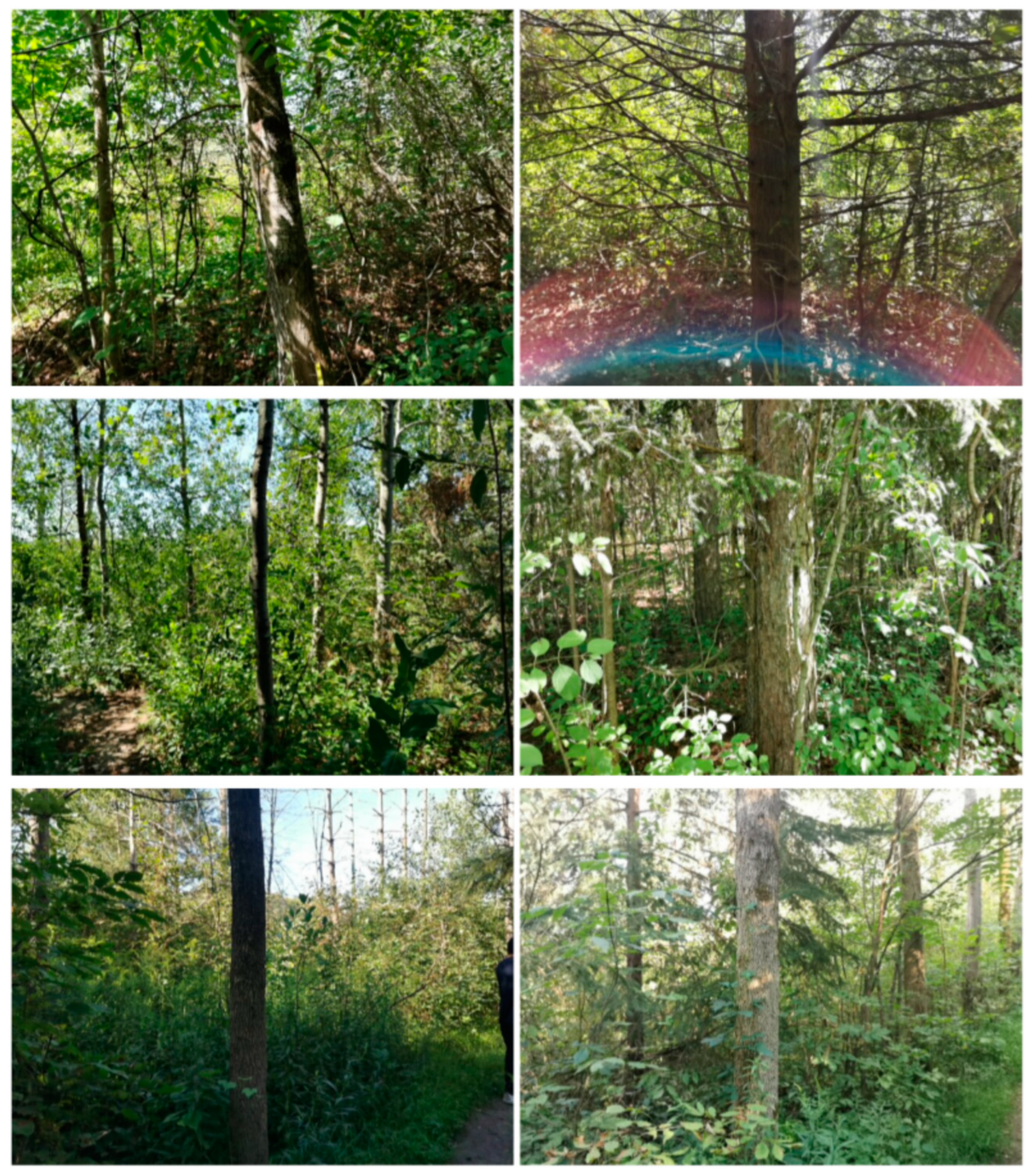
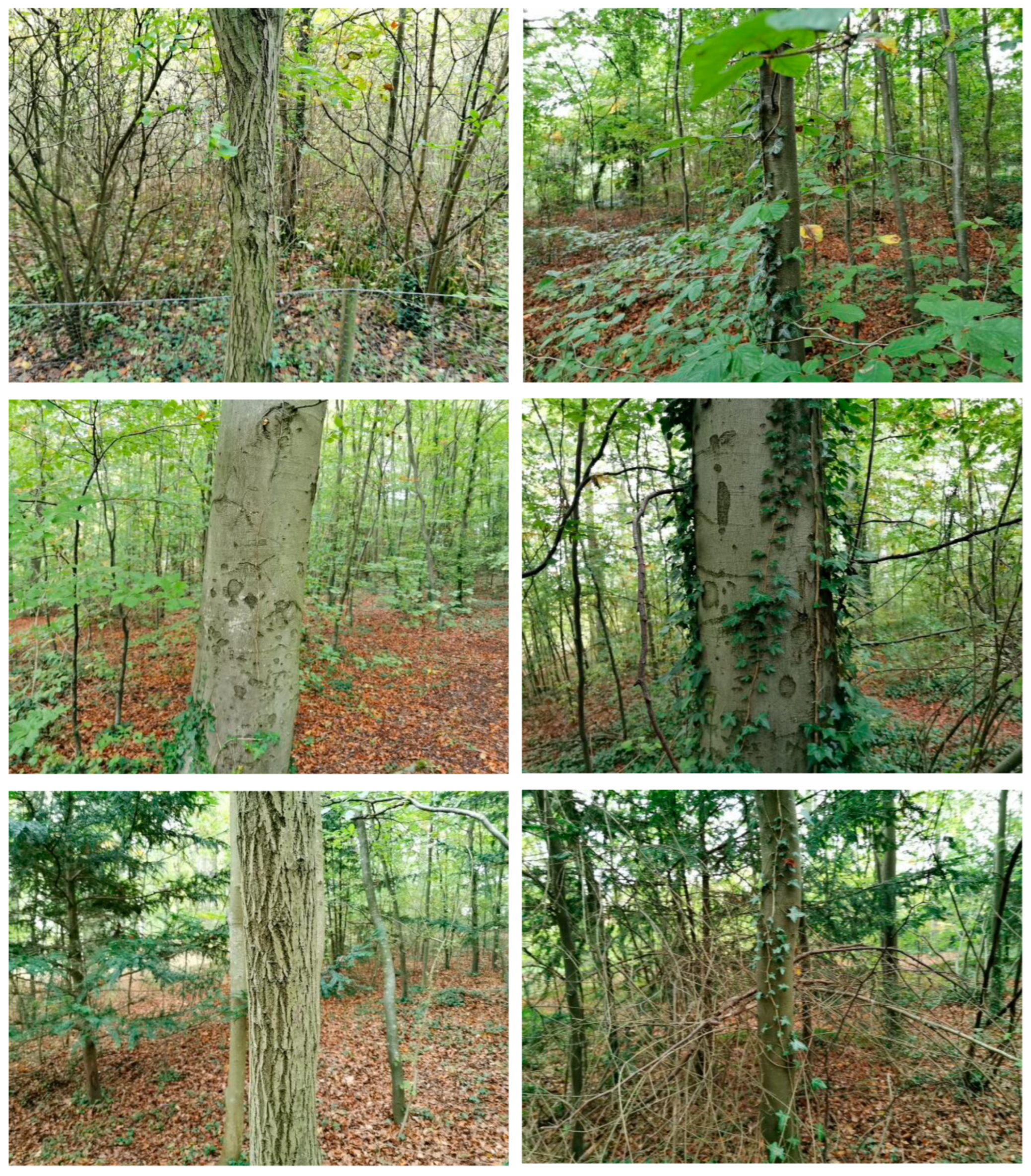
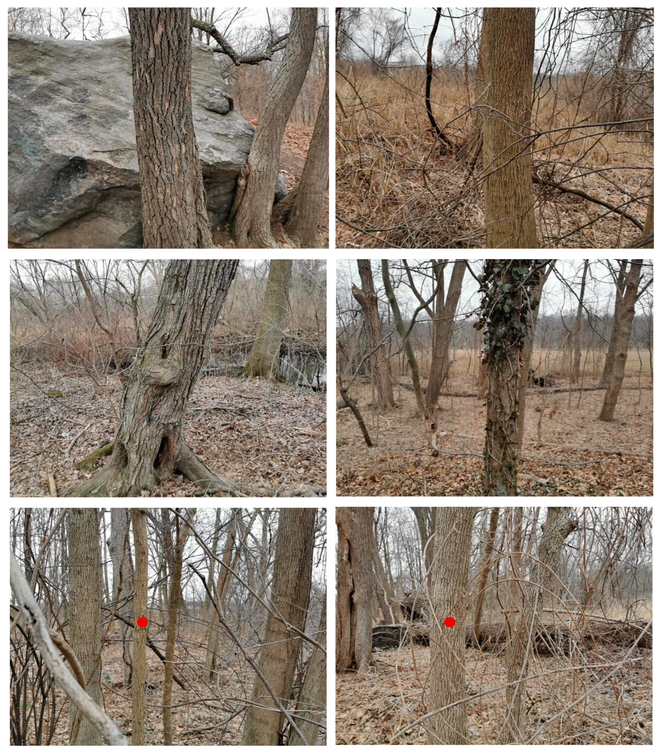
Appendix A.6. Sample Images

This supplement displays sample images from the Laurel Creek (Figure A3), Beechwoods (Figure A4), and Van Cortlandt (Figure A5) evaluation data sets.
Figure A3. Sample RGB images from the Laurel Creek data set, all taken from roughly 2 m away. The images in the left column are categorized as “low” occlusion because they have few to no branches and leaves in front of the trunk. The images in the right column were categorized as “medium“ or “high” occlusion. In addition to occlusion, the branches, shrubs, and leaves also make it difficult to walk around the tree.
Remotesensing 15 00772 g0a3
Figure A4. Sample RGB images from the Beechwoods data set, all of which correspond to the last (“best attempt“) image of a trunk based on user interaction. The images in the left column are categorized as “low” occlusion because they have few to no leaves or branches in front of the target trunk. The images in the right column were categorized as “medium“ or “high” occlusion.
Remotesensing 15 00772 g0a4
Figure A5. Sample RGB images from the Van Cortlandt data set, all of which correspond to the last (“best attempt“) image of a trunk based on user interaction. The images in the left column are categorized as “low” occlusion because they have few to no leaves or branches in front of the target trunk. The images in the right column were categorized as “medium“ or “high” occlusion. In dense areas, a red dot highlights the target trunk. These do not appear in the original image.
Remotesensing 15 00772 g0a5

Appendix A.7. Processing of Outlier Image (1.04 m DBH)

Figure A6. Processing steps for the significant outlier in the Van Cortlandt data set.
Remotesensing 15 00772 g0a6

References

  1. Grimault, J.; Bellassen, V.; Shishlov, I. Key Elements and Challenges in Monitoring, Certifying and Financing Forestry Carbon Projects; Technical Report 58; Institute for Climate Economics (I4CE): Paris, France, 2018. [Google Scholar]
  2. Land Use: Policies for a Net Zero UK; Technical Report; Committee on Climate Change: London, UK, 2020.
  3. Mbatu, R.S. REDD+ research: Reviewing the literature, limitations and ways forward. For. Policy Econ. 2016, 73, 140–152. [Google Scholar] [CrossRef]
  4. Longo, M.; Keller, M.; dos Santos, M.N.; Leitold, V.; Pinagé, E.R.; Baccini, A.; Saatchi, S.; Nogueira, E.M.; Batistella, M.; Morton, D.C. Aboveground biomass variability across intact and degraded forests in the Brazilian Amazon. Glob. Biogeochem. Cycles 2016, 30, 1639–1660. [Google Scholar] [CrossRef] [Green Version]
  5. Stovall, A.E.L.; Vorster, A.G.; Anderson, R.S.; Evangelista, P.H.; Shugart, H.H. Non-destructive aboveground biomass estimation of coniferous trees using terrestrial LiDAR. Remote Sens. Environ. 2017, 200, 31–42. [Google Scholar] [CrossRef]
  6. Schlegel, B.; Gayoso, J.; Guerra, J. Manual de Procedimentos para Inventarios de Carbono en Ecosistemas Forestales. Available online: https://www.ccmss.org.mx/wp-content/uploads/2014/10/Manual_de_procedimiento_para_inventarios_de_carbono_en_ecosistemas_forestales.pdf (accessed on 1 November 2022).
  7. Calders, K.; Adams, J.; Armston, J.; Bartholomeus, H.; Bauwens, S.; Bentley, L.P.; Chave, J.; Danson, F.M.; Demol, M.; Disney, M.; et al. Terrestrial laser scanning in forest ecology: Expanding the horizon. Remote Sens. Environ. 2020, 251, 112102. [Google Scholar] [CrossRef]
  8. Disney, M.; Boni Vicari, M.; Burt, A.; Calders, K.; Lewis, S.; Raumonen, P.; Wilkes, P. Weighing trees with lasers: Advances, challenges and opportunities. Interface Focus 2018, 8, 20170048. [Google Scholar] [CrossRef] [PubMed] [Green Version]
  9. Wilkes, P.; Lau, A.; Disney, M.; Calders, K.; Burt, A.; Gonzalez de Tanago, J.; Bartholomeus, H.; Brede, B.; Herold, M. Data acquisition considerations for Terrestrial Laser Scanning of forest plots. Remote Sens. Environ. 2017, 196, 140–153. [Google Scholar] [CrossRef]
  10. Fan, Y.; Feng, Z.; Mannan, A.; Khan, T.U.; Shen, C.; Saeed, S. Estimating Tree Position, Diameter at Breast Height, and Tree Height in Real-Time Using a Mobile Phone with RGB-D SLAM. Remote Sens. 2018, 10, 1845. [Google Scholar] [CrossRef] [Green Version]
  11. Çakir, G.Y.; Post, C.J.; Mikhailova, E.A.; Schlautman, M.A. 3D LiDAR Scanning of Urban Forest Structure Using a Consumer Tablet. Urban Sci. 2021, 5, 88. [Google Scholar] [CrossRef]
  12. Mokroš, M.; Mikita, T.; Singh, A.; Tomaštík, J.; Chudá, J.; Wężyk, P.; Kuželka, K.; Surový, P.; Klimánek, M.; Zięba-Kulawik, K.; et al. Novel low-cost mobile mapping systems for forest inventories as terrestrial laser scanning alternatives. Int. J. Appl. Earth Obs. Geoinf. 2021, 104, 102512. [Google Scholar] [CrossRef]
  13. Tatsumi, S.; Yamaguchi, K.; Furuya, N. ForestScanner: A mobile application for measuring and mapping trees with LiDAR-equipped iPhone and iPad. Methods Ecol. Evol. 2022. [Google Scholar] [CrossRef]
  14. Pace, R.; Masini, E.; Giuliarelli, D.; Biagiola, L.; Tomao, A.; Guidolotti, G.; Agrimi, M.; Portoghesi, L.; Angelis, P.D.; Calfapietra, C. Tree Measurements in the Urban Environment: Insights from Traditional and Digital Field Instruments to Smartphone Applications. Arboric. Urban For. 2022, 48, 2. [Google Scholar] [CrossRef]
  15. Gollob, C.; Ritter, T.; Kraßnitzer, R.; Tockner, A.; Nothdurft, A. Measurement of Forest Inventory Parameters with Apple iPad Pro and Integrated LiDAR Technology. Remote Sens. 2021, 13, 3129. [Google Scholar] [CrossRef]
  16. Piermattei, L.; Karel, W.; Wang, D.; Wieser, M.; Mokroš, M.; Surový, P.; Koreň, M.; Tomaštík, J.; Pfeifer, N.; Hollaus, M. Terrestrial Structure from Motion Photogrammetry for Deriving Forest Inventory Data. Remote Sens. 2019, 11, 950. [Google Scholar] [CrossRef] [Green Version]
  17. Katam Technologies AB. KATAM™ Forest. 2020. Available online: https://www.katam.se/solutions/forest/ (accessed on 31 March 2021).
  18. Rehman, H.Z.U.; Lee, S. Automatic Image Alignment Using Principal Component Analysis. IEEE Access 2018, 6, 72063–72072. [Google Scholar] [CrossRef]
  19. Wu, K.; Otoo, E.; Shoshani, A. Optimizing Connected Component Labeling Algorithms; Lawrence Berkeley National Laboratory: Berkeley, CA, USA, 2005. [Google Scholar]
  20. Ayari, T.; Radufe, N. Sony’s 3D Time of Flight Sensing Solution in the Huawei P30 pro; Technical Report SP20518; SystemPlus Consulting: Nantes, France, 2020. [Google Scholar]
  21. Yoshida, J. P30 Pro Teardown Proves Huawei’s Flash Catch-Up. 2019. Available online: https://www.eetimes.eu/p30-pro-teardown-proves-huaweis-flash-catch-up/ (accessed on 1 November 2022).
  22. Waldron, G.E. Trees of the Carolinian Forest; Boston Mills Press: Erin, ON, Canada, 2003. [Google Scholar]
  23. Ren, Q. Fuzzy Logic-based Digital Soil Mapping in the Laurel Creek Conservation Area, Waterloo, Ontario. Master’s Thesis, University of Waterloo, Waterloo, ON, Canada, 2012. [Google Scholar]
  24. The Wildlife Trust for Bedfordshire, C.a.N. Beechwoods. Available online: https://www.wildlifebcn.org/nature-reserves/beechwoods (accessed on 24 October 2021).
  25. Taylor, C. Most Wanted Invasive Plant Species in Our Natural Areas. Van Cortlandt Park Alliance 2018. Available online: https://vancortlandt.org/2018/11/08/most-wanted-invasive-plant-species-in-our-natural-areas/ (accessed on 31 March 2021).
  26. United States Geological Survey; National Geospatial Program US Topo: Yonkers, NY, USA, 2019; GNIS Cell Id: 50117. Available online: https://apps.nationalmap.gov/services/ (accessed on 16 January 2023).
  27. Liang, X.; Hyyppä, J.; Kaartinen, H.; Lehtomäki, M.; Pyörälä, J.; Pfeifer, N.; Holopainen, M.; Brolly, G.; Francesco, P.; Hackenberg, J.; et al. International benchmarking of terrestrial laser scanning approaches for forest inventories. ISPRS J. Photogramm. Remote Sens. 2018, 144, 137–179. [Google Scholar] [CrossRef]
  28. Gollob, C.; Ritter, T.; Nothdurft, A. Forest Inventory with Long Range and High-Speed Personal Laser Scanning (PLS) and Simultaneous Localization and Mapping (SLAM) Technology. Remote Sens. 2020, 12, 1509. [Google Scholar] [CrossRef]
  29. Paul, K.I.; Larmour, J.S.; Roxburgh, S.H.; England, J.R.; Davies, M.J.; Luck, H.D. Measurements of stem diameter: Implications for individual- and stand-level errors. Environ. Monit. Assess. 2017, 189, 416. [Google Scholar] [CrossRef]
  30. Liu, C.; Xing, Y.; Duanmu, J.; Tian, X. Evaluating Different Methods for Estimating Diameter at Breast Height from Terrestrial Laser Scanning. Remote Sens. 2018, 10, 513. [Google Scholar] [CrossRef] [Green Version]
  31. Srinivasan, S.; Popescu, S.C.; Eriksson, M.; Sheridan, R.D.; Ku, N.W. Terrestrial Laser Scanning as an Effective Tool to Retrieve Tree Level Height, Crown Width, and Stem Diameter. Remote Sens. 2015, 7, 1877–1896. [Google Scholar] [CrossRef] [Green Version]
  32. Hyyppä, J.; Virtanen, J.P.; Jaakkola, A.; Yu, X.; Hyyppä, H.; Liang, X. Feasibility of Google Tango and Kinect for Crowdsourcing Forestry Information. Forests 2018, 9, 6. [Google Scholar] [CrossRef] [Green Version]
Figure 1. An intuitive and simple user interface facilitates rapid capturing and validation of collected data. (Left) The app display shows the main camera preview. White lines help the user to center the tree in the frame. The ‘Capture’ button saves the current frame and initiates the image processing algorithm. (Right) After clicking ‘Capture’, the app highlights in green the detected trunk boundaries from which it will estimate diameter. The user is prompted to ‘Save’ the image, or else ‘Redo’ if the algorithm does not appear to have captured the tree correctly.
Remotesensing 15 00772 g001
Figure 2. A four-step algorithm filters, orients, and segments captured images before estimating trunk diameter. The steps are demonstrated in the sample image (a), with the RGB image on the left and the raw depths overlaid on the right. The roughly segmented depth image ( I s ) is shown in (b), and the sub-steps of filtering and orienting the image to obtain a highly filtered image I f and the trunk’s principal axis are displayed in (ce). The fitted trunk boundaries are shown in (f).
Remotesensing 15 00772 g002
Figure 3. User assistance improves the trunk detection rate to 100% in the Beechwoods and Van Cortlandt data sets. The box lines show the 25th, 50th, and 75th percentiles of the measurement error distribution. The plot whiskers show two times the interquartile range, and outliers are data points outside of this range. Outliers highlighted in red are those in which the algorithm failed to detect the trunk: at least one of the identified boundary lines does not correspond to the trunk in any way.
Remotesensing 15 00772 g003
Figure 4. DBH measurements are in good agreement with app diameter estimates ( R 2 = 0.97). The red dashed line shows a linear fit to the data, and the black line shows perfect correlation (reference DBH = estimated diameter).
Remotesensing 15 00772 g004
Figure 5. The designed app can estimate diameter without the surveyor touching the trunk, which speeds up measurement time for low-branching trees. Left, a small stand of cedars. Right, an image of the trunk taken by phone held just under the tree canopy.
Remotesensing 15 00772 g005
Figure 6. Circle-fitting is not straightforward for images taken in complex forest environments. Left: Raw depth image on which our app is able to estimate tree diameter with <1 cm of error. Center: RGB image with the green line indicating an estimated diameter line cross-sectioning the trunk. Right: Depth points are projected into real-world (x, z) coordinates (meters) along the cross-section identified in the center image. A circle-fitting approach would attempt to estimate a bounding circle for the trunk based on these points.
Remotesensing 15 00772 g006
Table 1. Summary of evaluation data sets.
NameLocationSeasonLeaf-on?No. SamplesDiameter Range
Laurel CreekWaterloo, ON, CanadaSummerY288–33 cm
BeechwoodsCambridge, UKAutumnY426–75 cm
Van CortlandtNew York, NY, USAWinterN296–105 cm
Table 2. Error distribution.
Data SetNo. SamplesRMSE (cm)Mean AbsoluteBias (cm)Mean abs. % Error
Error (cm)
Laurel Creek262.21.50.28.2
Beechwoods423.02.11.18.1
Van Cortlandt295.32.80.27.5
Combined973.72.20.68.0
Van Cortlandt * 282.72.01.16.9
Combined * 962.71.90.97.8
* With the outlier discussed in Section 5 removed.
Disclaimer/Publisher’s Note: The statements, opinions and data contained in all publications are solely those of the individual author(s) and contributor(s) and not of MDPI and/or the editor(s). MDPI and/or the editor(s) disclaim responsibility for any injury to people or property resulting from any ideas, methods, instructions or products referred to in the content.

