Article

Vicarious CAL/VAL Approach for Orbital Hyperspectral Sensors Using Multiple Sites

by
Daniela Heller Pearlshtien
1,*,
Stefano Pignatti
2 and
Eyal Ben-Dor
1
1
Remote Sensing Laboratory, Geography Department, Porter School of the Environment and Earth Sciences, Faculty of Exact Sciences, Tel Aviv University, Tel Aviv 699780, Israel
2
National Research Council (CNR), Institute of Methodologies for Environmental Analysis (IMAA), 85050 Potenza, Italy
*
Author to whom correspondence should be addressed.
Remote Sens. 2023, 15(3), 771; https://doi.org/10.3390/rs15030771
Submission received: 30 November 2022 / Revised: 22 January 2023 / Accepted: 23 January 2023 / Published: 29 January 2023
(This article belongs to the Special Issue Accuracy and Quality Control of Remote Sensing Data)

Abstract

:
The hyperspectral (HSR) sensors Earth Surface Mineral Dust Source Investigation (EMIT) of the National Aeronautics and Space Administration (NASA) and Environmental Mapping and Analysis Program (EnMAP) of the German Aerospace Center (DLR) were recently launched. These state-of-the-art sensors have joined the already operational HSR sensors DESIS (DLR), PRISMA (Italian Space Agency), and HISUI (developed by the Japanese Ministry of Economy, Trade, and Industry METI and Japan Aerospace Exploration Agency JAXA). The launching of more HSR sensors is being planned for the near future (e.g., SBG of NASA, and CHIME of the European Space Agency), and the challenge of monitoring and maintaining their calibration accuracy is becoming more relevant. We proposed two test sites: Amiaz Plain (AP) and Makhtesh Ramon (MR) for spectral, radiometric, and geometric calibration/validation (CAL/VAL). The sites are situated in the arid environment of southern Israel and are in the same overpass coverage. Both test sites have already demonstrated favorable results in assessing an HSR sensor’s performance and were chosen to participate in the EMIT and EnMAP validation stage. We first evaluated the feasibility of using AP and MR as CAL/VAL test sites with extensive datasets and sensors, such as the multispectral sensor Landsat (Landsat5 TM and Landsat8 OLI), the airborne HSR sensor AisaFENIX 1K, and the spaceborne HSR sensors DESIS and PRISMA. Field measurements were taken over time. The suggested methodology integrates reflectance and radiometric CAL/VAL test sites into one operational protocol. The method can highlight degradation in the spectral domain early on, help maintain quantitative applications, adjust the sensor’s radiometric calibration during its mission lifetime, and minimize uncertainties of calibration parameters. A PRISMA sensor case study demonstrates the complete operational protocol, i.e., performance evaluation, quality assessment, and cross-calibration between HSR sensors. These CAL/VAL sites are ready to serve as operational sites for other HSR sensors.

1. Introduction

Sensors, in general, and hyperspectral (HSR) sensors in particular, require periodic radiometric and spectral calibration. Both the calibration and validation of orbital sensors are critical processes in keeping their data reliable for thematic mapping during their operational lifetime, which is especially important in the challenging space environment [1]. Moreover, both the spectral calibration and the sensor’s optics can degrade over time, affecting the sensor’s spectral profile [2]. Thus, monitoring the spectral performance and radiometric stability periodically throughout the sensor’s lifetime is important to ensure accurate products [3].
With the recent launch of HSR sensors such as the Earth Surface Mineral Dust Source Investigation (EMIT) of the National Aeronautics and Space Administration (NASA) [4] and the Environmental Mapping and Analysis Program (EnMAP) of the German Aerospace Center (DLR) [5] into space, and the increasing number of HSR sensors already in orbit, calibration of the following advanced sensors is vital for the high spectral resolution that they provide: DLR Earth Sensing Imaging Spectrometer (DESIS); PRecursore IperSpettrale della Missione Applicativa (PRISMA) of the Italian Space Agency (ASI); the spaceborne hyperspectral earth imaging system (HISUI) developed by the Japanese Ministry of Economy, Trade and Industry and installed on the International Space Station (ISS) with the collaboration of the Japan Aerospace Exploration Agency (JAXA) module; India’s Hyper Spectral Imager (HySIS); and China’s Advanced Hyperspectral Imager (AHSI).
Technological advances have been made in the last decade, and the number of spectral bands and spectral ranges has increased to cover most of the sun’s radiation. Yet, separating the signals from noise to retrieve reliable physical data remains a complex procedure and requires the maintenance of an accurate sensor and post-calibration process, which is an ongoing challenge [6]. Aside from onboard calibration routines (such as partial-aperture calibrators, standard lamps, and solar diffuser panels [7]), vicarious calibration (VC) practices are important for examining and rectifying the sensor’s radiometric and spectral response, and checking its geometric performance [8]. VC comprises techniques that use natural or artificial sites for the post-launch calibration of sensors. It is a significant part of any satellite’s lifetime, and space agencies and groups worldwide (e.g., the IEEE P4001, the GEO, CAL/VAL Working Groups of Surface Biology and Geology (SBG) [9], and the RadCalNet [3,10]) are investing much effort in the calibration/validation (CAL/VAL) mission.
There are a few methods to apply VC using lunar views and bright stars, e.g., [11,12,13,14]. However, such targets are relatively low radiation sources [15], and they require high-risk spacecraft-platform maneuvers [7]. Other VC methods use non-land earth targets, including atmospheric Rayleigh scattering and gas absorption [16,17,18,19], and ocean sunglint [20]. However, the most common way to carry out VC is to use natural ground targets on earth, such as a uniform bright playa [21], and snow and ice fields [22,23,24]. The VC is applied over a well-known ground site that is stable in space and time. The measurement is conducted during or close to the sensor’s overpass time, estimating the top of the atmosphere (TOA) radiance at-sensor.
Aside from examining, and, in some cases, also rectifying a given sensor’s radiometric performance, another important practice at VC sites is the cross-calibration of two sensors. Cross-calibration uses data from a well-calibrated sensor to harmonize the information of a less-well-calibrated sensor [25,26,27]. Cross-calibration is performed on a stable test site (spatially, temporally, and spectrally) that is captured by the sensors at near-simultaneous times [21]. The test sites are referred to as pseudo-invariant calibration test sites (PICS). The main constraint of the cross-calibration approach is to find pairs of scenes for the calibration between two sensors. This is not easy with multispectral sensors, and it is extremely difficult with HSR sensors. Each HSR sensor has its own revisit cycle, and both need to capture the test site without cloud coverage at approximately the same time (usually, up to 3 days apart [21], but for very stable targets, up to 6 days are considered [28]).
There are specific criteria to establish an area as a reliable CAL/VAL site. Radiometric test sites must be uniform in terms of the spectral signal with nearly Lambertian reflectance of the bright surface, have temporal stability over a large area, and be arid regions with a low probability of clouds, scarce vegetation coverage, and a high spectral reflectance (>0.3 for all bands) [24,29]. Spectral and thematic test sites need to have large pure targets with significant spectral signatures across the optical range, which are temporally stable and monitored with frequent ground measurements. There are several radiometric calibration sites worldwide that are recognized by the Committee on Earth Observation Satellites (CEOS)/Working Group on Calibration & Validation (WGCV), and the Infrared and Visible Optical Sensors subgroup (IVOS); six sites are located in the Sahara from Cosnefroy’s pseudo-invariant calibration sites’ list [30,31]. The four “RadlCalNet” radiometric calibration test sites equipped with automated ground instrumentation that provides continuous measurements of both surface reflectance and local atmospheric conditions for the derivation of TOA reflectance are located in the USA, France, China, and Namibia [3].
Twenty-six years ago, Cosnefroy et al. [31] identified 20 desert sites in North Africa and Saudi Arabia as the PICS for cross-calibration. In 2019, Bacour et al. [30] showed that they are still relevant. However, the six Saharan sites (Algeria 3, Algeria 5, Libya 1, Libya 4, Mauritania 1, and Mauritania 2) have one crucial disadvantage: they are logistically difficult to reach, hindering ground-truth characterization [30].
Satellite images undergo a geometric correction process to connect the image to the ground coordinates. There are various empirical and physically based approaches, and each satellite platform implements its preferred method [32]. Geolocation accuracy affects the quality of the final thematic product; as such, inspection and reporting on the spatial accuracy are strongly needed.
One way to rectify distorted images is to measure ground control points (GCPs) in the field from well-defined targets or high-resolution satellite images [33]. A few geometric calibrations fields are dispersed worldwide, such as the Tsukuba test field in Japan, the Finnish Geodetic Institute test field in Sjokulla, La Crau in France, and more. As with the satellite platforms, each space organization uses its own preferred method. Zheng et al. [34] suggested standardizing the geometric validation process and creating a unified test site for all agencies. To that end, they evaluated the geometric accuracy of the SPOT-6, Pleiades, ALOS, ZY-3, and TH sensors on the Xianning test field in China.
CAL/VAL test sites satisfying all of the calibration and inspection requirements are highly needed, especially for the high-quality HSR sensors. We, therefore, proposed two test sites that fulfill the CAL/VAL criteria to enable spectral, radiometric, geometric, and thematic evaluations. The Amiaz Plain (AP) is a homogeneous bright-surface playa (5 × 5 km) with high reflectance values (>0.4). Because vegetation is scarce and it is stable in space and time, it is proposed for sensors’ radiometric evaluation and cross-calibration (31°04′20.98″N, 35°22′14.83″E). Makhtesh Ramon (MR) is a unique site that is known for its geological formations, and its abundance of many different minerals with distinct spectral features across the 400–2500 nm region (30°36′35.23″N, 34°51′15.22″E). This area is perfect for spectral and thematic validation. The test sites are close to each other (50 km) and very easy to access using well-built roads for routine field measurements. They are situated in the Israeli desert, with a dry climate. Since they are both nature reserves, the landscape is undisturbed and preserved by park rangers. Furthermore, NASA’s AErosol RObotic NETwork (AERONET) [35] station is located in”SEDE-BOKER”, 20 km from MR and about 45 km from AP.
In this study, we evaluated the characteristics of both test sites using recent HSR data from airborne [36,37] and orbital sensors, accompanied by comprehensive ground-truth and field studies, toward the development of a protocol to monitor the quality assurance (QA) of the HSR data and their related processing chain from space.

2. Materials and Methods

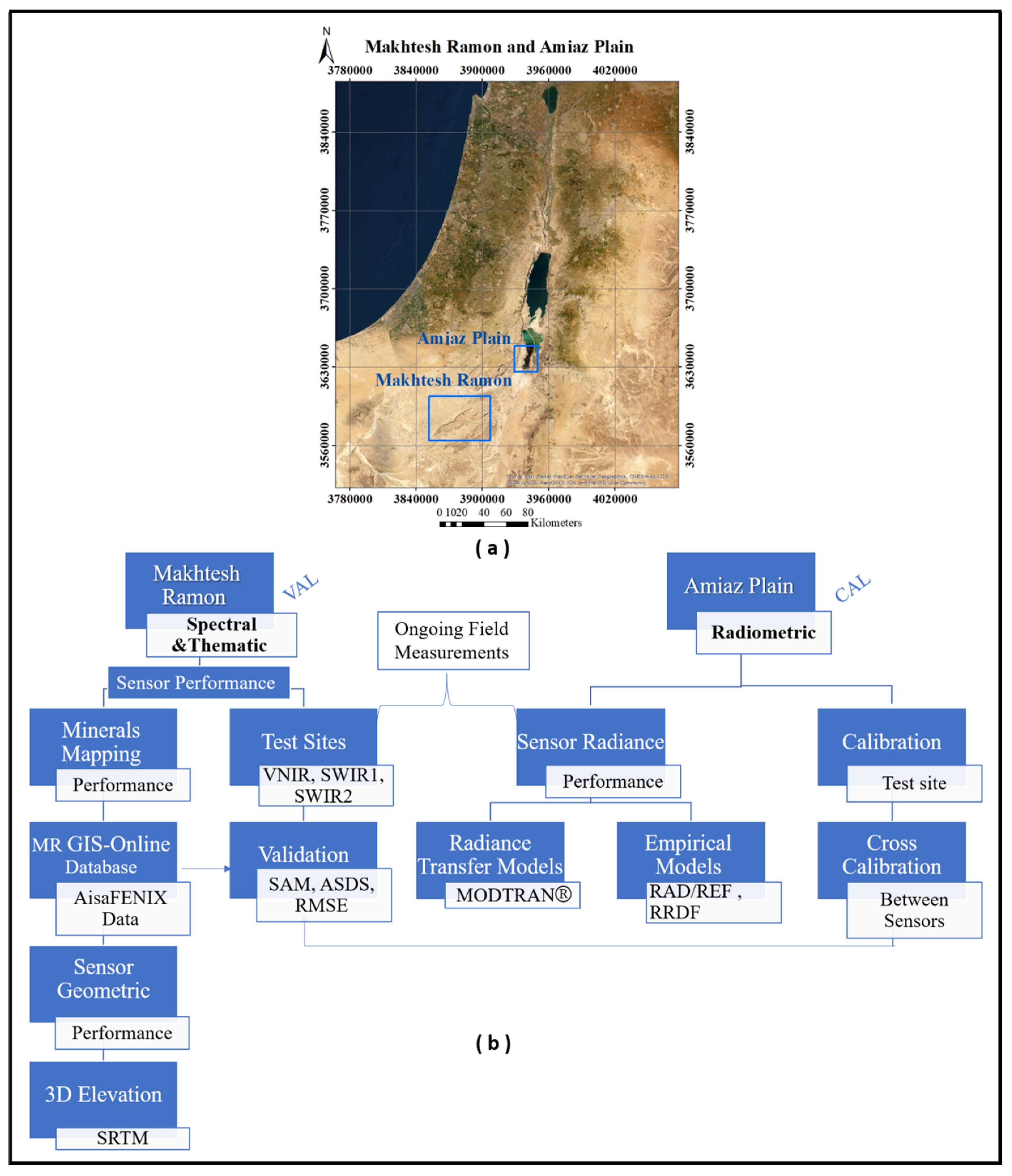
2.1. Test Sites AP and MR

Two areas were selected for the VC sites: AP and MR, located in the south of Israel (Figure 1a). AP is part of the Judean Desert Nature Reserve, and is located within a down-faulted block of the western segment of the Dead Sea fault system that bounds it from the west, and Mount Sodom bounds it from the east [38,39]. AP consists of a homogeneous silty carbonate plain with an elevation of about ~260 m below mean sea level. MR is an anticline formation with an eroded central valley occupying about 200 km². The surface valley elevation is about ~500 m above mean sea level, with steep walls that bound it. It is a natural geological park consisting of different geological formations with vast mineralogical exposures, such as dolomite, calcite, kaolinite, hematite, gypsum, montmorillonite, and more. Vegetation is scarce, and it has been widely documented in many geological and ecological studies.

2.2. Stability of the Test Sites

The most critical CAL/VAL site parameters are spatial and spectral stability over time. To evaluate these parameters for AP and MR, we gathered time-series analyses of Landsat images (Landsat-5 TM (TM5) and Landsat-8 OLI (OLI8)) over 20 and 25 years for AP and MR, respectively. We checked that no rain events had taken place at least 4 weeks before the overpass (this criterion was easily fulfilled due to the test sites’ arid climate). For a fair spectral comparison between the 2 different sensors (TM5 and OLI8), only 6 optical bands were used in the analysis (TM5—bands 1–5, 7 and OLI8—bands 2–7). All images were acquired during the summer season under dry conditions and clear skies. The spectral angle mapper (SAM; Equation (2)) [40], an algorithm that determines the spectral similarity between two spectra by calculating the angle between the spectra and treating them as vectors in a space with dimensionality equal to the number of bands; root mean square error (RMSE; Equation (3)); and the average sum of deviations squared (ASDS; Equation (4)) [41] were calculated between the t(0) and t(n) images, where n is the number of years after t(0). Lower values indicate higher spectral similarity.
R r n = R t n R t r n ,
S A M = c o s 1 ( i = 1 n R t n i R t r n i i = 1 n R t n i 2 i = 1 n R t r n i 2 ) ,
R M S E = i = 1 n ( R t r n i R t n i ) 2 n ,
A S D S = i = 1 n ( R r n i 1 ) 2 n ,
where R r n represents the ratio between the examined and reference spectra, R t n is the examined reflectance spectrum, R t r n is the reference reflectance spectrum, and n is the number of wavelengths used.
For the spatial examination, we used the “Change Detection Difference Map” method in the ENVI 5.6 program to produce a change-classification image. The difference was computed by subtracting the initial-state image from the final-state image, and the red band (0.66 µm) was selected for the analysis. For AP, t(0) = the year 2000 and t(n) = 2021, and for MR, t(0) = 1996, and t(n) = 2021 (see Section 3.1).

2.3. CAL/VAL Protocol Flowchart

The AP test site was selected to evaluate the sensor’s radiance performance and conduct the VC/cross-calibration. The sensor’s radiance calibration was evaluated by observing the wavelengths of atmospheric water vapor and trace gases at the sensor’s TOA radiance signal. The main absorbances for water vapor (H2O) are: 720, 820, 940, 1150, 1380, and 1870 nm; for oxygen (O2): 680 and 760 nm; for ozone (O3): 550 and 650 nm; for carbon dioxide (CO2): 2005 and 2060 nm; and for methane: 1660 nm and 2300 nm [30,42,43]. In this study, the simulated TOA radiance transfer signal was obtained using the MODTRAN® version 4 code [42,43], surface reflectance, and the precise atmospheric conditions measured at the AERONET station in Sede Boker. The sensor’s TOA signal was compared to the TOA radiance transfer model. Empirical indices—at-sensor radiance-to-reflectance ratio (RAD/REF) and radiance-to-reflectance difference factor (RRDF) [44]—can also be operated as QA indicators for radiance quality (see elaboration in our previous work [36]). We also used this test site for cross-calibration between HSR sensors DESIS, PRISMA, and AisaFENIX (see Section 3.2.3 and Section 3.2.4).
MR was used for the spectral QA, validation of atmospheric correction, cross-calibration, and geometric accuracy. The validation process was conducted on MR’s online database obtained from comprehensive field measurements and precise airborne HSR AisaFENIX flight products. It included thematic mineral maps of kaolinite, bentonite, hematite, goethite, calcite, and gypsum, and auxiliary MR data, such as geology/geomorphology maps of the area, slope, aspect maps, and a 3D elevation model (created from the SRTM 30 m resolution image of NASA–JPL at a resolution of 1 arc [45]). All of the thematic information, including updated field measurements, is uploaded into the cloud to be utilized by interested parties. Examples of using this database to examine the mapping performance of HSR sensors DESIS and PRISMA are demonstrated in our previous work [36,37]. The MR database is available at the following link: https://storymaps.arcgis.com/stories/bb5bf09ec7414454a012bfe9bf4b8545 (accessed on 11 October 2022) [46].
The main requirement for the reflectance validation test site is that the spectral response be stable in space and time. Accordingly, 6 homogeneous test sites with unique spectral features across the sensor’s optical spectral range were used to evaluate the sensor’s spectral calibration and to validate the sensor’s radiometric re-calibration. The test sites encompassed targets with different spectral ranges: in the visible–near infrared (VNIR) spectral range of 400–1000 nm (Test Sites 1 and 2): 1. Brown questa, a sandstone enriched with iron oxides such as hematite and goethite, with main spectral features at 420–600 nm and 900–1000 nm (30°37′14.26″N, 34°50′32.13″E); 2. Laccolite mineral over a gypsum deposit, a gabbro mineral of plutonic rock, and the laccolite is a very dark target with small absorbance between 800 and 900 nm, a low albedo value (<0.20), and a mostly monotonous signal from 1000 to 2500 nm (30°36′12.23″N, 34°53′42.80″E); in the shortwave infrared (SWIR) 1 spectral range of 1450–1800 nm (Test Sites 3 and 4): 3. Gypsum old mine with sulfate mineral deposits, and a distinctive absorbance of gypsum in that range (30°35′42.24″N, 34°52′21.13″E,); 4. Soil fans, also rich in gypsum (30°36′7.45″N, 34°53′37.08″E); for the SWIR2 spectral range of 2000–2500 nm (Test Sites 5 and 6): 5. Kaolinite old mine (clay mineral), main spectral feature at 2200 nm (30°37′19.85″N, 34°51′0.77″E); 6. Calcite (carbonate) layer, main spectral feature at 2340 nm (30°36′19.72″N, 34°51′49.18″E). Figure 2 shows the average spectral signature and photos of each MR validation test site.
To examine the sensor’s spectral accuracy, we compared the orbital sensor’s spectra to those of the airborne AisaFENIX and the field ground-truth spectra measured by an Analytical Spectral Devices (ASD) spectroradiometer at each test site. We considered the highly accurate AisaFENIX data to be our benchmark in the validation routine. For that purpose, we resized the AisaFENIX data cube to the sensors’ spatial and spectral configuration. The spectral similarity was calculated using SAM (Equation (2)) [40], RMSE (Equation (3)), and ASDS (Equation (4)) [41]. Lower values indicated higher spectral similarity, and the threshold values for good spectral calibration deduced from this study were SAM < 0.1, RMSE < 0.05, and ASDS < 0.1.
In addition, the sensor’s geometric accuracy was evaluated by looking at time-series images on well-formed geology targets and roads in MR images (200 points) along with field GPS measurements (see Section 3.2.5). The overall CAL/VAL protocol flowchart for radiometric, spectral, geometric, and thematic assessment is given in Figure 1b.

2.4. Field Measurements

Ongoing field measurements have been carried out at both the MR and AP sites since 2019. We followed the same field protocol at each test site, i.e., 6 MR VAL test sites (Figure 3a) and the CAL test site in AP (Figure 3b), including GPS, spectral measurements, soil sampling, and digital photos. An ASD FieldSpec® model FSP 350–2500 nm spectroradiometer was used for the spectral measurements in the field. The idea of the field protocol was to simulate a pure 1 pixel of a 30 m spatial resolution sensor. At each test site, approximately 32 points were taken along 30 m² (CAL and VAL), measuring the reflectance and/or radiance. An X-shaped grid was used (Figure 3c), with 10 measurements for each 30 m line, and then another 12 randomly added measurements around this X shape. The average of all 32 points represented the test site spectral signal (an example for AP is shown in Figure 3d). The GPS coordinates were measured at both ends and the center of each line.
In the case of a satellite with lower spatial resolution (for example, NASA’s EMIT with 60 m resolution), we adjusted the grid measurements to simulate a larger pixel: 60 × 60, 90 × 90, etc. It is important to mention that the selected area for the ground-truth measurement covered the most homogeneous flat terrain in the area to minimize any effect of bidirectional reflectance distribution function (BRDF), and the standard deviation of the average spectral reflectance was less than 5%. Table 1 summarizes the general information for each test site (Figure 3(a,b)).

2.5. Cross-Calibration of HSR Orbital Sensors Using AP Site

Cross-calibration transfers the calibration of a well-calibrated sensor, referred to (in this study) as the motherhood sensor, to a less-well-calibrated sensor. Radiometric calibration is performed using the TOA radiance or TOA reflectance signal. The advantage of using the reflectance values lies in reducing image-to-image variability; it removes the effect of different solar zenith angles and solar irradiance due to the time difference between data acquisitions. Each sensor has a different relative spectral response (RSR), which needs to be normalized by a factor so that the reflectance can be compared. The simulated TOA reflectance is calculated for each sensor by integrating the hyperspectral profile of the surface with the sensor’s RSR at each wavelength, weighted by the RSR of the respective sensor. The integral in the numerator calculates the amount of in-band reflectance acquired in the respective RSR and is divided by the integral of the RSR of the sensor, so that there is no gain/loss due to the filter response function. The spectral band adjustment factor (SBAF) is computed from the ratio of the 2 respective simulated sensors’ reflectances (Equation (5)). The SBAF is applied to the sensor’s original TOA reflectance for calibration (Equation (6)) [21,26,28]. The HSR sensors used in the study were well-calibrated for radiance, as determined by a prior examination conducted by both the space agencies and the authors [36,37]. Moreover, the cross-calibration result (SBAF method) of PRISMA with DESIS using the TOA reflectance did not result in any significant changes for PRISMA (3.2% standard deviation between the original to calibrated PRISMA signal). This led us to our next step, in which the SBAF method was applied on the surface reflectance (obtained from ASI and DLR products) in a cross-calibration exercise for the atmospheric models using AP as a PICS. Both PRISMA and DESIS level 2 atmospheric processors convert TOA spectral radiance into spectral reflectance by using a multidimensional look-up table (LUT) approach with MODTRAN code (6 for PRISMA and 5.4 DESIS). This stage is important for judging the quality of the L2 products over two adjacent sites (AP and MR) spectrally and thematically, to estimate how these two sensors perform together. For the purpose of this exercise, the following parameters were applied to Equation (5):
S B A F = p   ( M ) p   ( A ) = ρ ƛ h   R S R ( M ) d ƛ R S R ( M ) d ƛ ρ ƛ h   R S R ( A ) d ƛ R S R ( A ) d ƛ ,
where RSR (M) and RSR (A) are the relative spectral responses for the reference (motherhood) sensor and the sensor to be calibrated; p (A) is the simulated reflectance for sensor A to be calibrated; p (M) is the simulated reflectance for the well-calibrated sensor M; and ρλh is the accurate hyperspectral reflectance profile of the surface.
p ( A ) = p ( A ) × S B A F ,
where P′ (A) is the new reflectance for sensor A using the SBAF to match the reflectance of sensor M.
We examined the AP site for cross-calibration, calibrating the PRISMA sensor with DESIS and the AisaFENIX (see Section 3.2.3 and Section 3.2.4). The “reflectance” used in this study consisted of the average reflectance values of the AP scene obtained directly from the sensor’s atmospherically corrected products.

2.6. Sensors’ Image Data

A list of the sensor images used in this study is summarized in Table 2. It includes sensor parameters, the number of images, and the purpose of using the selected image.

3. Results

3.1. AP and MR Stability

Spatial and spectral change detection offers a straightforward approach to measuring changes between a pair of images that represent an initial and final state. The test sites’ spectral stability and spatial stability were examined using USGS Landsat Collection level 2 surface reflectance for Landsat TM5 and OLI8. Seven time-series images from 2000 to 2021 for AP and eight from 1996 to 2021 for MR were selected as representations of that time, all in the summer season. For AP, t(0) = 2000 and t(n) = 2021; for MR, t(0) = 1996, and t(n) = 2021.
Figure 4 shows the spatial change detected from 2000 to 2021 (green pixels); the red box indicates the AP calibration test site area. The Dead Sea area had low anthropogenic activity and is situated in an extreme desert environment; the only significant changes detected were structural and in the water levels of the evaporated ponds of the Dead Sea salt factory. Most of the terrestrial area in general, and the AP area in particular, did not change, remaining stable over 21 years.
Figure 5a shows a comparison of the mean Landsat reflectance spectra for the years 2000–2021. An average of 200 pixels in each year were used for the comparison. The SAM, ASDS, and RMSE were calculated against the year 2000 (t0) to examine possible spectral reflectance changes. The results are summarized in Figure 5b. The average values of SAM, ASDS, and RMSE were very low (Figure 5a), and these low values were maintained across the years: SAM 0.01–0.04, ASDS 0.0004–0.005, and RMSE 0.008–0.04. Although the spectral resolution was relatively low (six bands), it could be concluded that the spectral reflectance across the 21 years was very stable.
The change detection applied to AP was also applied to MR. In Figure 6, the result of the spatial changes detected in MR for the years 1996–2021 (red pixels) is provided. A significant change was detected over the town of Mizpe Ramon, situated on MR’s northern cliff (marked in a dashed green circle). This was mainly due to the massive urban buildup activity in the town in those years. Within the MR crater itself, there were a few changed areas (marked in a turquoise dashed circle). Those changes were part of the Natural Reserve Authority’s restoration activities (mostly between 1998 and 2000) to make MR accessible to the public as a touristic National Reserve park. Two camping areas were built, equipment was evacuated from the old mines, and new roads were constructed. The six spectral VAL test sites (marked by yellow Xs) and most of the crater remained stable over 20 years and are expected to remain so in the future.
To examine possible changes in the spectral reflectance of the six test sites at MR, a comparison of the mean Landsat reflectance for the years 1996–2021 was conducted (Figure 7). The SAM, ASDS, and RMSE values were calculated against the year 1996 (t0) at each test site, and the results are shown in Figure 8.
A very good match was obtained between all spectra in all MR VAL test sites, presenting very low average values of SAM, ASDS, and RMSE: 0.025–0.05, 0.001–0.01, and 0.009–0.018, respectively. The lowest values were obtained for the brown questa and gypsum fans, and the highest values for the kaolinite and laccolite sites. The changes in the laccolite (darkest test site) were mainly in the blue band. However, there was a small variation in the reflectance spectra within the test sites over the years. This may be a result of using different sensors in the calculations (TM5 and OLI8 (from 2015)), where a dark test site is more susceptible to the change (e.g.light dust). Nevertheless, the values are below the significance threshold for good data quality (i.e., SAM < 0.1, ASDS < 0.1, and RMSE < 0.05), indicating high spectral similarity and stability of the reflectance signal over the years.

3.2. AP and MR CAL/VAL Protocol: A Case Study Using the PRISMA HSR Sensor

The working protocol from Figure 1b is described in the following section with the PRISMA sensor as a case study. We used the 15 collected PRISMA images of AP and MR (2019–2022) in the case study analysis. A field campaign accompanied the November 2021 overpass images; therefore, some of the examples focus on those images.

3.2.1. Evaluate Radiance Performance

On 11 and 24 November 2021, images of AP and MR were acquired by PRISMA and transferred to us by ASI. Field spectral (radiance and reflectance) measurements were taken on 16 November, 2021.
We compared the L1 TOA PRISMA product to a radiance transfer model to evaluate the radiance performance. The TOA radiance model for AP was generated with the MODTRAN4 radiance transfer code and the ASD field reflectance spectrum. Atmospheric and solar radiation was generated to yield simulated TOA radiance values for the PRISMA spectral configuration overpass information (11 November, 2021, azimuth angle 160.8°, zenith angle 50.8°, day of the year 315, desert aerosol, sensor height 615 km); sky conditions, optical depth, and water vapor content were taken from the “SEDE BOKER” AERONET station (water vapor 1.27, angstrom exponent 0.997, ozone 0.2, and coarse /fine AOD in total 0.169). A comparison of the simulated radiance signal (mW m² sr¹ nm¹) and the real PRISMA L1 product signal is shown in Figure 9.
Figure 9 presents the TOA radiance signal of PRISMA (L1) and the simulated TOA radiance using the MODTRAN4 code. In both spectra, the absorbance positions of several gases well-matched their position in the MODTRAN radiance: O2 at 680 and 760 nm; O3 at 651 nm; H2O at 823, 940, and 1131 nm; and CO2 at 2010 and 2061 nm. There was a slight albedo offset between the PRISMA (L1) and MODTRAN radiance spectra of about 20 mW m² sr¹ nm¹ in the visible (VIS) spectral range (400–700 nm). This may be caused by the overfitting of the model when we tried to compensate for AP’s topographic elevation of 260 m below mean sea level (the MODTRAN code cannot calculate height below zeroin the model). Regardless, the overall shape and signals were mostly similar.

3.2.2. Evaluate Spectral Performance—PRISMA L2 Product

The PRISMA L2D (atmospherically corrected surface reflectance product) was evaluated at MR in six VAL test sites (Table 1) to determine PRISMA’s spectral calibration performance. A comparison of the sensor signal against the ground truth is an early warning step in identifying possible spectral calibration problems. “Problematic” bands were flagged for further examination.
It is important to mention that before generating the field-measurement protocol (Section 2.4), a homogeneous examination of the test sites was conducted. Different points (50–100) were randomly measured with a field ASD spectrometer at each test site. The average standard deviation (SD) was calculated for all of the spectral bands (excluding water vapor and the end of the sensor bands, i.e., 2450–2500 nm) and for each spectral range: VNIR, SWIR1, and SWIR2. Table 3 summarizes the results and shows less than 5% deviation when looking at the average result for all bands (350–2450 nm). Moreover, deviation results for the specific spectral ranges showed the lowest SD values for the specific mineral connected to that site’s evaluation, i.e., brown questa and laccolite VNIR SD < 0.02, gypsum mine and fans SWIR1 SD < 0.05, and kaolinite and calcite SWIR2 SD < 0.03. For the general evaluation, a comparison between the PRISMA reflectance and the average ASD ground truth was applied (Figure 10). Since PRISMA’s L2 atmospheric processor algorithm has changed many times since 2019, we used only five images (years 2021–2022) in the spectral evaluation. The mean reflectance for each MR VAL test site was calculated from the five images of PRISMA; in each image, 10 pixels from the six test sites were obtained from the location at which the field measurements were taken.
The flagged areas of concern (marked in black boxes, Figure 10) from the initial examination of PRISMA were in the VNIR range wavelengths, 920–970 nm, and 1100–1163 nm. This was probably caused by residual atmospheric absorbance (water vapor), which was not entirely removed in the atmospheric correction of the L2D product [47]. The exchange of PRISMA’s VNIR to SWIR sensor, which was in this range, may also have contributed. The SWIR2 range above 2320 nm showed a high deviation from the ASD signal; there was a sharp decrease in the spectra, and the calcite absorbance at 2340 nm shifted. This indicates that the performance of the atmospheric correction algorithm applied by the standard L2D processor for the SWIR2 bands is questionable.
For a deeper evaluation of the spectral calibration, the MR test sites were divided into specific spectral ranges: VNIR, SWIR1, and SWIR2, according to the major mineral at each VAL site (VNIR—brown questa (iron oxide) and laccolite; SWIR1—gypsum; SWIR2—kaolinite, and calcite). The spectral similarity between PRISMA and AisaFENIX was determined by calculating the SAM, RMSE, and ASDS separately for each range. For that purpose, the AisaFENIX data cube was resized to the 30 m spatial resolution and re-sampled to PRISMA’s spectral configuration. It should be noted that the use of AisaFENIX as a benchmark to examine the HSR performance from MR was already established and demonstrated by Heller-Pearlshtien et al. [36].
Table 4 summarizes the results for SAM, ASDS, and RMSE between the PRISMA and AisaFENIX spectra, for each VAL test site-specific spectral range (VNIR, SWIR1, and SWIR2), where PRISMA was the examined reflectance spectrum, and AisaFENIX the reference reflectance spectrum. Lower SAM, ASDS, and RMSE values indicate the similarity between the PRISMA and AisaFENIX spectral signatures. The highest values obtained were for the SWIR2 range (i.e., Test Sites 5 and 6, kaolinite and calcite), which were higher than the threshold for good spectral calibration (SAM and ASDS < 0.1, RMSE < 0.05). They were also considerably higher than the VNIR and SWIR1 test site results (Table 4). We also included the SAM, ASDS, and RMSE results for the entire spectral range (VNIR-SWIR (VSWIR) 400–2400 nm) in Table 4. The spectra differed from VNIR to SWIR, and were much larger at certain test sites. Hence, the potentially problematic spectral bands may be masked by the well-calibrated ones. For example, the result for the calcite test site does not reflect the deterioration after 2300 nm. Therefore, separation into specific spectral ranges in the evaluation is critical. This result and the initial spectral inspection strengthen the suspicion that the PRISMA’s SWIR2 spectral bands are less well-calibrated and should be used with caution [47].
It is important to mention that an entire article was dedicated to examining PRISMA’s mineral mapping capability (i.e., goethite, hematite, gypsum, kaolinite, and calcite) and validated against the airborne AisaFENIX database [36]. It was concluded that the sensor provides a very accurate spectral-based mapping of minerals over the MR site (excluding a poor result for the calcite mineral). Therefore, this step in the CAL/VAL protocol was excluded from the current paper.

3.2.3. Cross-Calibration and Validation between PRISMA and DESIS Level-2 Products

Cross-calibration between spaceborne sensors can be achieved by using PICS. These sites are chosen for their high surface homogeneity and spectral, spatial, and temporal stability [30]. AP was found to be a very stable area over 20 years (Section 3.1); therefore, it can be used as a vicarious calibration test site and for cross-calibration as a PICS. In this section, we conducted a cross-calibration between PRISMA and DESIS on the atmospheric-correction models obtained from their products (i.e., PRISMA L2D, DESIS L2A) using their shared spectral region, i.e., the VNIR range. The images were captured over AP 3 days apart (PRISMA 3 June, 2021, 8:26 UTC, and DESIS 30 May, 2021, 8:53 UTC). The DESIS sensor had 235 bands in the VNIR spectral range (400–1000 nm) and 30 m ground sampling distance (GSD), and was found in previous work to perform well (above 450 nm) [37]. The PRISMA sensor had 63 bands (450–998 nm) and 30 m GSD. The simulated reflectance for each sensor was obtained by integrating the AisaFENIX hyperspecral profile of the AP surface with the sensor’s RSR. Beforehand, the DESIS and AisaFENIX spectral signals were converted to PRISMA’s VNIR 63-band configuration. The SBAF was obtained by dividing the sensor’s simulated reflectance (Equation (5)), which was then operated on PRISMA’s original L2D signal, to create a new reflectance (Equation (6)). The calculation was created by implementing the following data into Equations (5) and (6):
  • p (sensor A)—simulated reflectance for the sensor to be calibrated (PRISMA);
  • p (sensor M)—simulated reflectance for the well-calibrated (motherhood) DESIS sensor;
  • ρλh—AisaFENIX’s accurate hyperspectral reflectance profile of the surface.
The result of the PRISMA cross-calibration in AP (VNIR bands) is shown in Figure 11: the original (before cross-calibration) PRISMA L2D spectral signal (black line) against the newly calibrated signal (blue line), and the ground-truth field ASD reflectance (dashed red line).
We calculated the RMSE of PRISMA’s VNIR signal to validate our result. The RMSE decreased from 8% to 3% after the cross-calibration (Figure 11a), thereby improving the reflectance signal accuracy for PRISMA’s VNIR bands.
To further validate the cross-calibration result, we applied the AP’s SBAF to PRISMA’s image of MR (taken at the same time as the AP image). MR’s brown questa test site had the most pronounced spectral signature in the VNIR range due to the rich iron-oxide composition. Figure 11b shows the result of applying AP’s SBAF on PRISMA’s brown questa signal after calibration (blue line) against the original signal (black line), and the ground-truth ASD spectrum (dashed red line). Though the brown questa spectra from the original PRISMA signal, the calibrated signal, and the ASD spectra were similar, it can be seen that the noticeable artifacts in the original L2D signal (before calibration, black line) at 900–1000 nm were less pronounced after the cross-calibration (blue line).

Uncertainty Analysis

Different sources of uncertainty influence the cross-calibration accuracy, including the inherent variability of the sensors, and the process and techniques involved in the measurement [21]. In this study, the SBAF was calculated with only one pair of images (not a dataset), showing the potential of the cross-calibration method using PRISMA and DESIS over the AP CAL site. Consequently, the calculation of uncertainty was limited. We considered the following parameters as the main sources of uncertainty: the site’s spatial variability (non-uniformity), the sensors’ temporal drift (when capturing the site area), and the calibration model error. The site’s spatial variability uncertainty (σ² spatial) manifested both the spatial and temporal drift components and was obtained by calculating the mean of the standard deviation of each sensor’s region of interest (AP test site area) reflectance (i.e., PRISMA, DESIS, and AisaFENIX, Equation (7)). The calibration model uncertainty (σ2 calibration) was calculated by the RMSE of the model to predict the surface reflectance, which is the predicted reflectance against the measured ASD ground-truth reflectance at each wavelength (Equation (8)). The obtained total uncertainty for the cross-calibration model (Equation (9)), combined from the above, was 0.047.
Uncertainty σ   s p a t i a l   = ( σ 2 s p a t i a l ( A ) + σ 2 s p a t i a l ( M ) + σ 2 s p a t i a l ( p h ) )   ,
Uncertainty σ   c a l i b r a t i o n = i = 1 n ( A S D n i   P r e d i c t n i ) 2 n ,
Uncertainty   σ   total =   σ 2 s p a t i a l + σ 2 c a l i b r a t i o n ,
Uncertainty   σ   total =   ( s p a t i a l ( 0.015 2 + 0.023 2 + 0.024 2 ) + c a l i b r a t i o n ( 0.03 ) 2 )   = 0.047  
where n is 63, the number of wavelengths used for the cross-calibration; A is PRISMA; M is DESIS; and ph is AisaFENIX.

3.2.4. Cross-Calibration against a Fixed High-Quality Sensor Image

The main constraint of classical cross-calibration is finding pairs of scenes that have been captured within a short time interval (up to 6 days in a stable PICS). This is easier with multispectral sensors, but enormously difficult with HSR sensors. Each HSR sensor has its own revisit cycle, and both need to capture the test site with no cloud cover. It may take a long time to accumulate dozens of datasets.
A potential solution to this is to perform an empirical cross-calibration process with a fixed high-quality motherhood sensor, where the HSR images are not captured simultaneously, and to use reflectance to reduce the effect of the different time acquisitions (such as solar irradiance, solar zenith angles, and variation in the earth–sun distance). Accurate ground-truth measurements of the test site, to be integrated into the calculation of the sensors’ simulated reflectance (motherhood and the sensor to be calibrated), can help normalize the signals for the time difference. Needless to say, the areas should not undergo surface changes in each overpass.
Accordingly, we performed a cross-calibration of PRISMA’s sensor with the well-calibrated AisaFENIX HSR airborne data as the motherhood (calibrated) sensor, using four PRISMA images of AP. The field ASD measurements provided an accurate spectral profile of the test site.
We re-sampled the AisaFENIX and ASD spectral signals to PRISMA’s 220-band configuration (400–2500 nm, excluding water vapor bands), and re-sized AisaFENIX to a 30 m spatial resolution. The SBAF (Equation (5)) was calculated for four different PRISMA AP images dated April, June, November, and December 2021, implementing the following:
  • p (sensor A)—simulated reflectance for PRISMA (to be calibrated);
  • p (sensor M)—simulated reflectance for the well-calibrated (motherhood) sensor AisaFENIX;
  • ρλh—ASD field hyperspectral profile of the surface (resampled to PRISMA bands).
The simulated reflectance for each sensor (PRISMA and AisaFENIX) was obtained by integrating the ASD profile with their RSRs. The SBAF was obtained by dividing the sensor’s simulated reflectance.
The SBAFs for each band, resulting from the cross-calibration of PRISMA with AisaFENIX, are shown in Figure 12. The averaged SBAF is indicated by a black line, the gain factors ranged between 0.97 and 1.78 up to wavelength 2350 nm, and the values increased above this wavelength. The average standard deviation for all bands’ SBAFs was 13%. The high variation implies that the dataset is not large enough to create a generic SBAF for PRISMA’s images; more images are needed. Still, the SBAF for each month can be used to calibrate PRISMA’s images near their timeline.
To validate the concept of this method, we applied the November AP SBAF on the original PRISMA AP image. Figure 13 shows the result for the November image: the original PRISMA L2D (before calibration) signal (black line) against the calibrated SBAF (blue line), and the ground-truth ASD (dashed red line). The artifacts in the VNIR bands (900–1000 nm) were removed, and the absorbance at 2340 nm (carbonates) was better obtained in the PRISMA signal after the calibration. The RMSE of the calibrated November signal against the ASD reflectance was 0.05 vs. the original (L2D product before calibration) 0.15. The total σ uncertainty for the model was calculated from Equations (7)–(9), where n is 220, the number of wavelengths used for the cross-calibration; A is PRISMA (sensor to be calibrated); M is AisaFENIX (well-calibrated sensor); and ph is ASD, and was 0.06.
Uncertainty   total   σ   = σ 2 S p a t i a l + σ 2 c a l i b r a t i o n   = S p a t i a l [ ( P R I S M A ( 0.015 ) 2 + A S D ( 0.020 ) 2 + A I S A ( 0.023 ) 2 ) ] + c a l i b r a t i o n ( 0.05 ) ²   = 0.060
To further validate the SBAF model, the AP’s November SBAF was applied to the MR’s November PRISMA image (acquired at the same time). The SAM, ASDS, and RMSE of the calibrated PRISMA reflectance (blue line, Figure 14) against the field ASD reflectance (dashed black line, Figure 14) were calculated. The results for the six MR VAL test sites are presented in Figure 14.
After applying the SBAF, the corrected reflectance well-matched the field ASD spectra in most test sites. The SAM results in all test sites had values <0.1 (the threshold for good spectral calibration). For the ASDS and RMSE, all test site results were below the threshold (ASDS < 0.1, RMSE < 0.05) except for Test Sites 2 (laccolite) and 6 (calcite) (Figure 14b,f), and the ASDS value for Test Site 1 (Figure 14a) was slightly higher from the thresholds (value of 0.107). This is because even though the signals for Test Sites 1, 2, and 6 were similar to the ASD, the RMSE and ASDS were more susceptible to albedo differences than the SAM.
Overall, the calibrated results for the model were good; the artifacts in the PRISMA’s original VNIR signal (around 900–1000 nm) decreased, especially in Test Site 1 (brown questa; Figure 14a, marked by box). Another significant impact of the SBAF correction can be seen in the calcite (Test Site 6; Figure 14f, marked by box), where the significant deterioration across the end of SWIR2 of PRISMA was well-corrected and the calcite main absorbance feature at 2340 nm was back to its theoretical position.

3.2.5. Evaluate Sensor’s Thematic Stability

The geometric rectification of an image is an essential stage in geolocating surface targets and generating an accurate thematic map. The performance of the sensor’s geometric correction is crucial when time-series images are used, either from the same sensor or when different sensors are integrated. MR’s unique geological formations are stable in time, visually well-defined, and can be exploited to evaluate the geometric accuracy of an image. Accordingly, we examined the geometric precision performance of PRISMA’s sensor over 4 years of operation (2019–2022). In general, PRISMA declares a geolocation accuracy of 200 m [32], whereas ASI is intended to provide a better-rectified product of up to 15 m using well-defined GCPs.
Four PRISMA MR images (one per year) were used. In each image, 200 randomly spread GCPs were selected across the image, and their location coordinates were compared to the previous year’s image. In addition, the initial and final years (2019, 2022) were examined for any drifts in the rectification process over 4 years of operation. The results are summarized in Table 5. Figure 15 and Figure 16 show examples of the geometric drift in the PRISMA image. Figure 15 shows the thematic change between the years 2019 and 2022 at MR. There was a shift of about 8 pixels (238 m) in the longitudinal direction and 3 pixels (95 m) in the latitudinal one. Several places are marked with red arrows to emphasize the drifts in 2019 (solid line) vs. 2022 (dashed line), such as the main road around the crater, basalt deposit, and dirt road. Figure 16 zooms in on three of our VAL test sites: kaolinite (top panels), gypsum soil fans, and laccolite (bottom panels). The red cross indicates the same coordinate position.
It can be seen that the highest drift occured between 2019 and 2022, and the least change in position was noticed between images 2019 and 2020. Still, the maximum drift stayed around PRISMA’s expected 200 m accuracy.

4. Discussion

The primary requirement for CAL/VAL test sites is that they be stable spectrally and spatially in space and time. We demonstrated that AP and MR fulfill this requirement using Landsat time-series images over 20 and 25 years, respectively. No spatial changes were detected across the years 2000–2021 at the AP CAL site (Figure 4). Furthermore, the spectral signals were stable in time as judged by the low values for SAM, ASDS, and RMSE (0.029, 0.002, and 0.023, respectively; Figure 5). At MR (VAL site), during the years 1996–2021, small spatial changes were observed due to restoration work toward establishing MR as a touristic nature park (Figure 6). However, this activity did not affect the geology or landscape of the six selected VAL test sites, as evidenced by the low values of SAM, ASDS, and RMSE (Figure 7 and Figure 8). It should be remembered that both AP and MR are located in desert areas where the sky is clear most of the year, vegetation is scarce, and precipitation is very limited (25 mm annually). Since both areas have been declared nature reserves, vigorous enforcement by rangers to keep the park’s landscape undisturbed means that only designated paths are available to tourists. Researchers require special permits to work in the park. This action will maintain the stability of the parks in the coming years. Other advantages are that both CAL/VAL sites can be captured in the same acquisition overpass, access to the sites is simple, and the distance between AP and MR is about a 1 h drive, enabling ground-truth measurements during or close to the overpasses. In addition, NASA’s AERONET station, which collects daily atmospheric aerosol data, is located at Sede Boker, close to both MR (20 km) and AP (45 km). These make AP and MR ideal areas for CAL/VAL sites: spectrally, spatially, and thematically.
We demonstrated the use of AP as a cross-calibration PICS between HSR sensors. Figure 11 shows the reflectance cross-calibration results between DESIS and the PRISMA VNIR bands, with an uncertainty of 0.047. After applying the SBAF calibration, the RMSE of the ground-truth ASD measurements against the original PRISMA L2D reflectance signal decreased from 8% to 3%.
It is important to note that in practice, TOA radiance or TOA reflectance information is used for cross-calibration between sensors. Our “cross-calibration” (SBAF method) was conducted using surface reflectance-calibrated products to demonstrate the advantages of using two adjacent sites: AP for reflectance cross-calibration examination, and MR for spectral cross-validation, which is actually a QA procedure of space agencies’ products and is vital to ensuring that the data from multiple sensors can be used to provide a consistent set of measurements. Still, in the operational process, dozens of pairs of images are used to create a generic SBAF between two sensors, and not just one pair, as done in this study. Gathering a dataset of HSR image pairs can be challenging and time-consuming. The images must be taken almost simultaneously with no clouds, while synchronizing the HSR sensors‘ revisit cycle.
Therefore, a new potential approach for cross-calibration against a fixed high-quality sensor when the images are not taken at the same time was presented. We used the well-calibrated AisaFENIX AP image as the benchmark and calibrated PRISMA’s AP images at different times. The SBAF was applied and validated on six MR (VAL) test sites, showing an improvement in the PRISMA’s calibrated signal: the artifacts in the original L2D PRISMA signal (900–1000 nm) were quite markedly diminished at the brown questa site (Figure 14a). Moreover, at the calcite site, the mineral spectral signature returned to its accurate position at 2340 nm (Figure 14f). PRISMA’s longer wavelength (SWIR2) demonstrated a significant variation from the field ASD measurement, suggesting that the PRISMA L2D performance in this spectral region should be regarded with caution. This is in accordance with the results of [47,48]. We showed only a primary result of this empirical fixed high-quality sensor cross-calibration method; further study and examination with different sensors and timelines are needed.
The geometric correction accuracy of HSR images is a fundamental parameter affecting the quality of the products. Scientists worldwide put effort into finding new validation methods for sensor geometric correction and increased precision. Because the HSR images are used for quantitative applications, their geometric accuracy is critical. For time-series applications, precision is crucial. MR’s stability with time enables the selecting of GCPs to check the geometric accuracy and rectify it. PRISMA’s images from 2019–2022 were examined, and the drifts between the geometric locations were calculated (Table 4). The highest shift was approximately 8 pixels (238 m) in the longitudinal direction and 3 pixels (95 m) in the latitudinal one (2019 to 2022), which is within the expected PRISMA accuracy of about 200 m. In the near future, ASI plans to improve the geometric precision to half a pixel by implementing GCPs in the geometric correction [32].
With this new era of launching sophisticated HSR sensors (e.g., EMIT, EnMAP, and DESIS), the demand for more accurate and challenging applications has increased. The HSR sensors need to provide high-end products that are strongly related to the quality of the retrieved reflectance and the radiance calibration of the sensors.
We performed a case study on ASI’s PRISMA sensor, demonstrating the unique combination of radiance (AP CAL site), reflectance, and thematics (MR VAL site) for monitoring, calibrating, and then validating sensor performance. Using these ideal CAL/VAL sites may improve the day-to-day utilization of HSR sensors while identifying problems first-hand, such as the deterioration of specific spectral wavelengths and radiance calibration, and rectifying them accordingly.

5. Conclusions

This research demonstrated that AP and MR are excellent sites for radiometric, spectral, and geometric/thematic validation and calibration. Both sites are very stable spectrally and spatially and can be used as CAL/VAL sites. AP is ideal for the vicarious radiometric calibration or pseudo-invariant calibration for cross-calibration between sensors. MR’s unique geological features, encompassing various minerals, are ideal for spectral assessment across the 400–2500 nm optical range. Six VAL test sites were found for the validation process, and the MR web database can be used to evaluate and validate the HSR sensor’s mapping performance. The advantage of using MR for determining the sensors’ geometric accuracy and stability was also established.
Using these dual test sites simultaneously can improve the assessment of HSR sensor radiance, and spectral and thematic performance. The suggested generic CAL/VAL protocol can help maintain a precise, accurate signal during the sensor’s mission lifetime, thus assisting in the challenge of maintaining the sensor’s high-end products.

Author Contributions

Conceptualization, D.H.P. and E.B.-D.; methodology, D.H.P. and E.B.-D.; software, D.H.P.; validation, D.H.P.; formal analysis, D.H.P. and E.B.-D.; investigation, D.H.P., S.P. and E.B.-D.; resources, S.P. and E.B.-D.; data curation, S.P. and D.H.P.; writing—original draft preparation, D.H.P. and E.B.-D.; writing—review and editing, D.H.P., E.B.-D. and S.P.; visualization, D.H.P.; supervision, E.B.-D.; funding acquisition, E.B.-D. and S.P. All authors have read and agreed to the published version of the manuscript.

Funding

This research was partially funded by the Israel Ministry of Science and Space project, grant number 3-17510, and by the Italian Space Agency ASI, PRISCAV project (grant agreement n. 2019-5-HH.0).

Data Availability Statement

The MR database developed for this study is available at the following link: https://storymaps.arcgis.com/stories/bb5bf09ec7414454a012bfe9bf4b8545 (accessed on 11 October 2022) [46].

Conflicts of Interest

The authors declare no conflict of interest.

References

  1. Mckenzie, I.; Karafolas, N. Fiber optic sensing in space structures: The experience of the European Space Agency (Invited Paper). In Proceedings of the 17th International Conference on Optical Fibre Sensors, Bruges, Belgium, 23 May 2005; Volume 5855, p. 262. [Google Scholar] [CrossRef]
  2. Chander, G.; Helder, D.L.; Aaron, D.; Mishra, N.; Shrestha, A.K. Assessment of spectral, misregistration, and spatial uncertainties inherent in the cross-calibration study. IEEE Trans. Geosci. Remote Sens. 2013, 51, 1282–1296. [Google Scholar] [CrossRef]
  3. Bouvet, M.; Thome, K.; Berthelot, B.; Bialek, A.; Czapla-Myers, J.; Fox, N.P.; Goryl, P.; Henry, P.; Ma, L.; Marcq, S.; et al. RadCalNet: A radiometric calibration network for earth observing imagers operating in the visible to shortwave infrared spectral range. Remote Sens. 2019, 11, 2401. [Google Scholar] [CrossRef] [Green Version]
  4. EMIT Homepage. Available online: https://earth.jpl.nasa.gov/emit/instrument/overview/ (accessed on 10 August 2022).
  5. EnMAP Homepage. Available online: https://www.enmap.org/ (accessed on 10 August 2022).
  6. Dubovik, O.; Schuster, G.L.; Xu, F.; Hu, Y.; Bösch, H.; Landgraf, J.; Li, Z. Grand Challenges in Satellite Remote Sensing. Front. Remote Sens. 2021, 2, 619818. [Google Scholar] [CrossRef]
  7. Thenkabail, P. Remote Sensing Handbook Volume 1: Remotely Sensed Data Characterized, Classification and Accuracies; Taylor & Francis Group, LLC: Abingdon, UK, 2016. [Google Scholar]
  8. Xu, H.; Zhang, L.; Huang, W.; Li, X.; Si, X.; Xu, W.; Song, Q. On-Board Absolute Radiometric Calibration and Validation Based on Solar Diffuser of HY-1C SCS. Guangxue Xuebao/Acta Opt. Sin. 2020, 40, 30015–30034. [Google Scholar] [CrossRef]
  9. CAL/VAL Working Groups—Surface Biology and Geology. Available online: https://sbg.jpl.nasa.gov/groups (accessed on 10 August 2022).
  10. RadCalNet Portal. Available online: https://www.radcalnet.org/#!/ (accessed on 22 July 2022).
  11. Kieffer, H.H.; Wildey, R.L. Absolute calibration of Landsat instruments using the moon. Photogramm. Eng. Remote Sens. 1985, 51, 1391–1393. [Google Scholar]
  12. Barnes, R.A.; Eplee, R.E.; Patt, F.S.; Kieffer, H.H.; Stone, T.C.; Meister, G.; Butler, J.J.; McClain, C.R. Comparison of SeaWiFS measurements of the Moon with the U.S. Geological Survey lunar model. Appl. Opt. 2004, 43, 5838–5854. [Google Scholar] [CrossRef] [PubMed] [Green Version]
  13. Kouyama, T.; Kato, S.; Kikuchi, M.; Sakuma, F.; Miura, A.; Tachikawa, T.; Tsuchida, S.; Obata, K.; Nakamura, R. Lunar calibration for ASTER VNIR and TIR with observations of the Moon in 2003 and 2017. Remote Sens. 2019, 11, 2712. [Google Scholar] [CrossRef] [Green Version]
  14. Kieffer, H.H.; Stone, T.C.; Barnes, R.A.; Bender, S.C.; Eplee, R.E., Jr.; Mendenhall, J.A.; Ong, L. On-orbit radiometric calibration over time and between spacecraft using the Moon. In Proceedings of the Sensors, Systems, and Next-Generation Satellites VI, Crete, Greece, 8 April 2003; Volume 4881, p. 287. [Google Scholar]
  15. Chang, I.-L.; Dean, C.; Li, Z.; Weinreb, M.; Wu, X.; Swamy, P.A.V.B. Refined algorithms for star-based monitoring of GOES Imager visible-channel responsivities. In Proceedings of the Earth Observing Systems XVII, San Diego, CA, USA, 15 October 2012; Volume 8510, p. 85100R. [Google Scholar]
  16. Vermote, E.; Santer, R.; Deschamps, P.Y.; Herman, M. In-flight calibration of large field of view sensors at short wavelengths using Rayleigh scattering. Int. J. Remote Sens. 1992, 13, 3409–3429. [Google Scholar] [CrossRef]
  17. Kaufman, Y.J.; Holben, B.N. Calibration of the AVHRR visible and near-IR bands by atmospheric scattering, ocean glint and desert reflection. Int. J. Remote Sens. 1993, 14, 21–52. [Google Scholar] [CrossRef]
  18. Robert, S.F.; Kaufman, Y.J. Calibration of satellite sensors after launch. Appl. Opt. 1986, 25, 1177–1185. [Google Scholar]
  19. Meygret, A.; Briottet, X.; Henry, P.J.; Hagolle, O. Calibration of SPOT4 HRVIR and Vegetation cameras over Rayleigh scattering. In Proceedings of the Earth Observing Systems V, San Diego, CA, USA, 15 November 2000; Volume 4135, p. 302. [Google Scholar]
  20. Luderer, G.; Coakley, J.A.; Tahnk, W.R. Using sun glint to check the relative calibration of reflected spectral radiances. J. Atmos. Ocean. Technol. 2005, 22, 1480–1493. [Google Scholar] [CrossRef]
  21. Khakurel, P.; Leigh, L.; Kaewmanee, M.; Pinto, C.T. Extended pseudo invariant site-based trend-to-trend cross-calibration of optical satellite sensors. Remote Sens. 2021, 13, 1545. [Google Scholar] [CrossRef]
  22. Loeb, N.G. In-flight calibration of NOAA AVHRR visible and near-IR bands over Greenland and Antarctica. Int. J. Remote Sens. 1997, 18, 477–490. [Google Scholar] [CrossRef]
  23. Tahnk, W.R.; Coakley, J.A. Updated calibration coefficients for NOAA-14 AVHRR channels 1 and 2. Int. J. Remote Sens. 2001, 22, 3053–3057. [Google Scholar] [CrossRef]
  24. Ling, W.; Xiuqing, H.; Yupeng, L.; Zhizhao, L.; Min, M. Selection and Characterization of Glaciers on the Tibetan Plateau as Potential Pseudoinvariant Calibration Sites. IEEE J. Sel. Top. Appl. Earth Obs. Remote Sens. 2019, 12, 424–436. [Google Scholar] [CrossRef]
  25. Kwiatkowska, E.J.; Franz, B.A.; Meister, G.; McClain, C.R.; Xiong, X. Cross calibration of ocean-color bands from Moderate Resolution Imaging Spectroradiometer on Terra platform. Appl. Opt. 2008, 47, 6796–6810. [Google Scholar] [CrossRef] [PubMed]
  26. Chander, G.; Mishra, N.; Helder, D.L.; Aaron, D.B.; Angal, A.; Choi, T.; Xiong, X.; Doelling, D.R. Applications of spectral band adjustment factors (SBAF) for cross-calibration. IEEE Trans. Geosci. Remote Sens. 2013, 51, 1267–1281. [Google Scholar] [CrossRef]
  27. Obata, K.; Tsuchida, S.; Yamamoto, H.; Thome, K. Cross-calibration between ASTER and MODIS visible to near-infrared bands for improvement of aster radiometric calibration. Sensors 2017, 17, 1793. [Google Scholar] [CrossRef] [Green Version]
  28. Barsi, J.A.; Alhammoud, B.; Czapla-Myers, J.; Gascon, F.; Haque, M.O.; Kaewmanee, M.; Leigh, L.; Markham, B.L. Sentinel-2A MSI and Landsat-8 OLI radiometric cross comparison over desert sites. Eur. J. Remote Sens. 2018, 51, 822–837. [Google Scholar] [CrossRef]
  29. Scott, K.P.; Thome, K.J.; Brownlee, M.R. Evaluation of Railroad Valley playa for use in vicarious calibration. In Proceedings of the Multispectral Imaging for Terrestrial Applications, Denver, CO, USA, 4 November 1996; Volume 2818, p. 158. [Google Scholar]
  30. Bacour, C.; Briottet, X.; Bréon, F.M.; Viallefont-Robinet, F.; Bouvet, M. Revisiting Pseudo Invariant Calibration Sites (PICS) over sand deserts for vicarious calibration of optical imagers at 20 km and 100 km scales. Remote Sens. 2019, 11, 1166. [Google Scholar] [CrossRef] [Green Version]
  31. Cosnefroy, H.; Leroy, M.; Briottet, X. Selection and characterization of Saharan and Arabian desert sites for the calibration of optical satellite sensors. Remote Sens. Environ. 1996, 58, 101–114. [Google Scholar] [CrossRef]
  32. Baiocchi, V.; Giannone, F.; Monti, F. How to Orient and Orthorectify PRISMA Images and Related Issues. Remote Sens. 2022, 14, 1991. [Google Scholar] [CrossRef]
  33. Berthelot, B.; Santer, R. Calibration Test Sites Selection and Characterisation Site Equipment and Auxiliary Data; Vega Technique SAS: Erstein, France, 2008. [Google Scholar]
  34. Zheng, X.; Huang, Q.; Wang, J.; Wang, T.; Zhang, G. Geometric accuracy evaluation of high-resolution satellite images based on Xianning test field. Sensors 2018, 18, 2121. [Google Scholar] [CrossRef] [Green Version]
  35. Aerosol Robotic Network (AERONET) Homepage. Available online: https://aeronet.gsfc.nasa.gov/ (accessed on 17 July 2022).
  36. Heller-Pearlshtien, D.; Pignatti, S.; Greisman-ran, U.; Ben-Dor, E. PRISMA sensor evaluation: A case study of mineral mapping performance over Makhtesh Ramon, Israel. Int. J. Remote Sens. 2021, 42, 5882–5914. [Google Scholar] [CrossRef]
  37. Heller-Pearlshtien, D.; Ben-Dor, E. CalVal Evaluation of DESIS products in Amiaz Plain and Makhtesh Ramon Test sites. In Proceedings of the 1st DESIS User Workshop—Imaging Spectrometer Space Mission, Calibration and Validation, Applications, Methods, Virtual, 28 September–1 October 2021; pp. 13–21. [Google Scholar]
  38. Zak, R.; Freund, R. Strain Measurements in Eastern Marginal Shear Zone of Mount Sedom Salt Diapir, Israel. Am. Assoc. Pet. Geol. Bull. 1980, 64, 568–581. [Google Scholar] [CrossRef]
  39. Weinberger, R.; Bar-Matthews, M.; Levi, T.; Begin, Z.B. Late-Pleistocene rise of the Sedom diapir on the backdrop of water-level fluctuations of Lake Lisan, Dead Sea basin. Quat. Int. 2007, 175, 53–61. [Google Scholar] [CrossRef]
  40. Kruse, F.A.; Lefkoff, A.B.; Boardman, J.W.; Heidebrecht, K.B.; Shapiro, A.T.; Barloon, P.J.; Goetz, A.F.H. The spectral image processing system (SIPS)-interactive visualization and analysis of imaging spectrometer data. Remote Sens. Environ. 1993, 44, 145–163. [Google Scholar] [CrossRef]
  41. Ben-Dor, E.; Kindel, B.; Goetz, A.F.H. Quality assessment of several methods to recover surface reflectance using synthetic imaging spectroscopy data. Remote Sens. Environ. 2004, 90, 389–404. [Google Scholar] [CrossRef]
  42. Kneizys, F.; Abreu, L.; Anderson, G.; Chetwynd, J.; Shettle, E.; Berk, A.; Bernstein, L.; Robertson, D.; Acharya, P.; Rothman, L.; et al. The MODTRAN 2/3 Report and LOWTRAN-7 Model; Contract F19628-91-C-0132; Ontar Corporation: North Andover, MA, USA, 1996. [Google Scholar]
  43. MODTRAN®. Available online: http://modtran.spectral.com/modtran_index (accessed on 15 September 2022).
  44. Brook, A.; Ben-Dor, E. Supervised vicarious calibration (SVC) of hyperspectral remote-sensing data. Remote Sens. Environ. 2011, 115, 1543–1555. [Google Scholar] [CrossRef]
  45. Farr, T.G.; Rosen, P.A.; Caro, E.; Crippen, R.; Duren, R.; Hensley, S.; Kobrick, M.; Paller, M.; Rodriguez, E.; Roth, L.; et al. The Shuttle Radar Topography Mission. Rev. Geophys. 2007, 45, RG2004. [Google Scholar] [CrossRef] [Green Version]
  46. Makhtesh Ramon Cal/Val Site. Available online: https://storymaps.arcgis.com/stories/bb5bf09ec7414454a012bfe9bf4b8545 (accessed on 23 July 2022).
  47. Pignatti, S.; Amodeo, A.; Carfora, M.F.; Casa, R.; Mona, L.; Palombo, A.; Pascucci, S.; Rosoldi, M.; Santini, F.; Laneve, G. PRISMA L1 and L2 Performances within the PRISCAV Project: The Pignola Test Site in Southern Italy. Remote Sens. 2022, 14, 1985. [Google Scholar] [CrossRef]
  48. Cogliati, S.; Sarti, F.; Chiarantini, L.; Cosi, M.; Lorusso, R.; Lopinto, E.; Miglietta, F.; Genesio, L.; Guanter, L.; Damm, A.; et al. The PRISMA imaging spectroscopy mission: Overview and first performance analysis. Remote Sens. Environ. 2021, 262, 112499. [Google Scholar] [CrossRef]
Figure 1. Amiaz Plain (AP) and Makhtesh Ramon (MR) calibration/validation (CAL/VAL) test sites. (a) AP and MR locations in Israel. (b) Work protocol flowchart.
Remotesensing 15 00771 g001
Figure 2. MR test sites. Different mineralogies and spectral signatures characterize the 6 test sites. Spectral signatures are from the spectral library acquired using an Analytical Spectral Devices (ASD) spectroradiometer.
Remotesensing 15 00771 g002
Figure 3. Location of test sites in (a) MR, and (b) AP. (c) Field spectral measurement protocol; example from the AP test site. (d) Average spectral signal (AVG, solid blue line) and standard deviation (SD, dashed black line) for AP 30 × 30 cube.
Remotesensing 15 00771 g003
Figure 4. Spatial change detection result for AP, 2000 vs. 2021. Test site is marked in a red box; detected changed pixels are colored in green (center image).
Remotesensing 15 00771 g004
Figure 5. Examination of spectral change in AP. (a) Mean Landsat reflectance signal for each year (2000–2021). (b) SAM, ASDS, and RMSE for each year against the year 2000 (t0).
Remotesensing 15 00771 g005
Figure 6. Spatial change detection result for MR, 1996 vs. 2021. Spectral test sites are marked by yellow Xs, detected changed pixels are colored in red.
Remotesensing 15 00771 g006
Figure 7. Examination of spectral changes at MR VAL test sites: LANDSAT reflectance signal for each year (1996–2021): (a) brown questa; (b) laccolite; (c) gypsum mine; (d) gypsum fans; (e) kaolinite; (f) calcite. The mean value is marked by black dashed lines.
Remotesensing 15 00771 g007
Figure 8. Spectral change examination. SAM, ASDS, and RMSE for each year against the year 1996 (t0).
Remotesensing 15 00771 g008
Figure 9. Radiance comparisons. TOA radiance from PRISMA L1 vs. MODTRAN simulation.
Remotesensing 15 00771 g009
Figure 10. Evaluation of PRISMA L2D spectra (PRI) vs. ASD at the six test sites (PRISMA—solid line, ASD ground truth—dashed line). BQ, brown questa; L, laccolite; GM, gypsum—mine; GF, gypsum—fans.
Remotesensing 15 00771 g010
Figure 11. (a) AP cross-calibration results for PRISMA (PRI); original (before calibration; black line), after SBAF cross-calibration (Cal, blue line) against ASD ground truth (red dotted line), ratio of original (ORI) to calibrated (green triangle). (b) Validation of AP SBAF on MR VNIR test site using brown questa (BQ).
Remotesensing 15 00771 g011
Figure 12. The spectral band adjustment factors (SBAFs) for PRISMA in different acquisition months (April—blue; June—orange; November—red; December—green; average SBAF—black).
Remotesensing 15 00771 g012
Figure 13. The AP cross-calibration result for PRISMA (PRI) with well-calibrated AisaFENIX; original reflectance (before calibration, black line), after SBAF calibration (blue line) against ASD ground truth (red dotted line).
Remotesensing 15 00771 g013
Figure 14. The MR test sites of PRISMA original (before calibration) reflectance (black line) against corrected reflectance (after applying the SBAF, blue line), and the field ASD spectra (dashed black line); (a) brown questa (BQ), (b) laccolite, (c) gypsum mine, (d) gypsum fans, (e) kaolinite, (f) calcite.
Remotesensing 15 00771 g014
Figure 15. Comparison of PRISMA’s 2019 and 2022 geometric corrections: (a) 2019 MR image; (b) 2022 MR image; (c) 2022 image overlaid on 2019 image. Several drifts in the geolocation are marked with red arrows (2019—solid; 2022—dashed).
Remotesensing 15 00771 g015
Figure 16. Comparison of the same coordinates (red cross) for the years 2019–2022 at three MR test sites: kaolinite (top panels), gypsum soil fans, and laccolite (bottom panels). There is a slight shift in the locations.
Remotesensing 15 00771 g016
Table 1. Test site information.
Test SiteNumberAltitude
(Meters Above Sea Level)
Area
(Square Meters)
MR Brown questa152128,241
MR Laccolite246917,262
MR Gypsum—old mine349881,473
MR Gypsum—soil fans446927,857
MR Kaolinite—old mine5502356,531
MR Calcite650348,578
AP7−2581,757,943
Table 2. Sensors and images used in the study.
SensorInformationNumber of ImagesPurpose
Landsat 5 Thematic Mapper 5 (NASA/USGS) 7 bands, spectral range visible (VIS)–SWIR 0.45–2.35 µm, 30 m GSD (ground sample distance); thermal infrared (TIR) 10.40–12.50 µm, 120 m GSD9Evaluation of spectral and spatial stability of MR and AP for years 1996–2011
Landsat 8 Operational Land Imager (NASA/USGS) 11 bands, spectral range VIS–SWIR 0.43–2.29 µm, 30 m GSD; TIR 10.60–12.51 µm, 100 m GSD; panchromatic 0.5–0.68 µm6Evaluation of spectral and spatial stability of MR and AP for years 2015–2021
PRISMA
PRecursore IperSpettrale della Missione Applicativa
Italian Space Agency (ASI)
234 bands, range of 400–2500 nm, 30 m GSD; full-width half maximum (FWHM) ≤12 nm, swath 30 km, sensor altitude 615 km
L1 TOA radiometric image, L2B ground radiometric image, and L2D atmosphere- corrected data cube. Acquired from PRISMA’s website
15Validation of CAL/VAL research protocols for AP and MR. Image dates: 2019–2022
DESIS
DLR Earth Sensing Imaging Spectrometer
German Aerospace Center (DLR)
235 bands, spectral range 400–1000 nm, 30 m GSD; FWHM ~3.5 nm, swath 30 km, sensor altitude 400 km. L1C radiometric georectified image and L2A atmosphere- corrected data cube.
Acquired from DESIS EOweb GeoPortal.
6Validation of CAL/VAL research protocols for AP and MR. Image dates: 2020–2021
AisaFenix 1K
(HSR sensor AisaFENIX—Specim, Spectral Imaging Ltd.)
An airborne campaign using the AisaFENIX 1K over MR and AP was carried out on April 5, 2017, covering the entire MR (200 km²) area and AP (5 km²). 420 bands, spectral range 375–2500 nm, 1.5 m GSD; FWHM: VIS 3.4 (nm), NIR–SWIR, 6.2 (nm), swath 1.8 km25 lines on MR
1 line on AP
Establishing high-accuracy reference data for AP and MR, mapping MR main minerals, and summarizing in an online database.
Benchmark data for the CAL/VAL protocol [36,46]
ASD FieldSpec
model FSP 350–2500 nm
(Model 3 and Model 4)
Spectral range of 350–2500 nm with 2151 bands, with 3 nm and 8 nm resolution for the VNIR and SWIR regionsOngoingIn-situ field measurements of radiance and reflectance for validation. Years 2019–2022
The Shuttle Radar Topography Mission (SRTM)NASA–JPL at a resolution of 1 arc-s (approximately 30 m) [45]1Creating 3D elevation models of MR.
Slope and aspect maps
Table 3. Homogenous evaluation of each test site for ASD field measurments (SD for each point set).
Test SiteNumber of ASD PointsSD VNIRSD SWIR1SD SWIR2SD All Bands
Brown questa620.01610.02500.02180.0180
Laccolite580.01170.01730.01610.0129
Gypsum—mine610.03520.05400.06270.0374
Gypsum—soil fans500.02070.02420.03180.0217
Kaolinite700.02260.03630.03390.0254
Calcite1090.02050.02220.02230.0224
Table 4. SAM, ASDS, and RMSE values for each test site.
Test SiteSpectral RangeWavelength (nm)SAMASDSRMSE
Brown questaVNIR402–9980.0890.0500.032
LaccoliteVNIR402–9980.0600.0200.020
Gypsum—mineSWIR11480–17940.0670.0710.027
Gypsum—soil fansSWIR11480–17940.0660.0730.042
KaoliniteSWIR22001–24000.1440.3000.103
CalciteSWIR22001–24000.1550.2800.098
Brown questaVSWIR400–24000.1280.2200.048
LaccoliteVSWIR400–24000.1030.2070.026
Gypsum—mineVSWIR400–24000.0890.1090.038
Gypsum—soil fansVSWIR400–24000.0920.1230.075
KaoliniteVSWIR400–24000. 1310.1800.083
CalciteVSWIR400–24000.1010.1230.042
Table 5. Shifts in longitudinal (X) and latitudinal (Y) location for 200 GCPs at MR, between years 2019 and 2022. Average error and standard deviation were calculated.
Years Compared X Error (m)Y Error (m)SD XSD Y
2019–202016.819.70.690.37
2020–2021243.166.90.751.13
2021–202216.918.30.430.23
2019–2022238.695.10.511.18
Disclaimer/Publisher’s Note: The statements, opinions and data contained in all publications are solely those of the individual author(s) and contributor(s) and not of MDPI and/or the editor(s). MDPI and/or the editor(s) disclaim responsibility for any injury to people or property resulting from any ideas, methods, instructions or products referred to in the content.

