Article

A Single-Hydrophone Coherent-Processing Method for Line-Spectrum Enhancement

1
Acoustic Science and Technology Laboratory, Harbin Engineering University, Harbin 150001, China
2
Key Laboratory of Marine Information Acquisition and Security (Harbin Engineering University), Ministry of Industry and Information Technology, Harbin 150001, China
3
College of Underwater Acoustic Engineering, Harbin Engineering University, Harbin 150001, China
*
Author to whom correspondence should be addressed.
Remote Sens. 2023, 15(3), 659; https://doi.org/10.3390/rs15030659
Submission received: 29 November 2022 / Revised: 13 January 2023 / Accepted: 19 January 2023 / Published: 22 January 2023
(This article belongs to the Special Issue Underwater Communication and Networking)

Abstract

:
Improving the line-spectrum detection capability of a single hydrophone is of great significance for the passive detection of small underwater platforms. In this paper, we propose a single-hydrophone cross-power spectrum (SHCS) method based on time-domain coherence. This method uses the coherence of the line spectrum and the non-coherence of the continuous spectrum noise to obtain coherent gain and improve the signal-to-noise ratio (SNR) of the line spectrum. The effects of the input SNR, number of averaging operations, and overlap ratio on the performance of the SHCS method under a background of Gaussian white noise are simulated and analyzed. The results show that when the overlap ratio is 0 and the number of averaging operations reaches saturation, the SHCS method can achieve the best performance and about 15 dB coherence gain is obtained. The performance of the SHCS method was verified by sea experiments. Under the extremely low input SNR, in which the line spectrum was almost completely submerged in the marine environmental noise, the SHCS method can obtain about 10 dB coherence gain. Under the conventional input SNR, in which the line spectrum could be observed, the SHCS method can obtain about 13 dB coherence gain. The results of processing the radiated noise from an actual cargo ship also demonstrate the effectiveness of the SHCS method.

1. Introduction

Underwater noise radiated from ships on the water is a significant component of low-frequency ambient noise (<100 Hz) in the ocean [1]. During actual navigation, the vibrations of the rotating machinery of a ship’s power system and propeller blades will inevitably result in the radiation of periodic noise that will spread to surrounding sea areas [2]. Usually, the noise radiated from a ship consists of a combination of a line spectrum and a continuum spectrum [3,4]. The line spectrum is an important part of this noise, and it describes the periodic part of the target radiated noise signal, such as the periodic noise generated by propellers and auxiliary machines [5,6]. A ship’s line spectrum is stable and can improve the detection distance of passive sonar [7]. Therefore, in passive-sonar signal processing, the detection and extraction of a ship’s line-spectrum features has always been a topic of intensive research in the field of underwater acoustics; it has important application value in the field of ocean observation and national defense. With the development of vibration- and noise-reduction technology, the noise levels radiated from ships have been greatly reduced and they continue to decrease. Improving the detection ability for weak signals is thus of great significance for detecting such quiet underwater targets [8]. The frequency characteristics of the line spectrum are related to the physical characteristics of the targets, which means it is an important feature for passive sonar target detection. Burenkov et al. [9] conducted an experimental study for the propagation characteristics of the line spectrum, and their results showed that a continuous wave (CW) signal with the features of a line spectrum can propagate for 9000 km and still retain a stable phase.
Generally, when attempting to enhance the signal-to-noise (SNR) ratios of sonar signals, designers target spatial or time processing gains [10]. Passive detection systems based on modern spectral-estimation algorithms (such as MUSIC [11] and ESPRIT [12]) all use array-processing methods. This approach can result in spatial processing gains, but it has problems such as high system overhead, difficult array design, and inflexible deployment, and these systems cannot be installed in the case of limited platform size. Small underwater platforms such as underwater gliders, unmanned underwater vehicles, and submersible buoy systems have the advantages of small size, flexibility, and easy concealment, and they are widely used in the field of underwater target detection. Generally, only a single hydrophone can be carried on these small platforms. Underwater target-detection methods based on a single hydrophone mainly use the line spectrum. The SNR of the line spectrum thus directly affects the detection capability of such passive sonar systems.
Researchers around the world have invested significant efforts to improve the line-spectrum detection capability of passive sonar. Firstly, the average periodogram method was proposed [13], which divides the received signal sequence into several segments, calculates the periodogram for each segment separately, and then takes the average of each periodogram as an estimate of the power spectrum. This method reduces the random fluctuations of the traditional periodogram method. Then, the Welch method [14], which combines windowing and average processing, was proposed. In the Welch method, the segmented data are multiplied by a window function, their periodograms are calculated separately, and then they are averaged. The spectral-estimation curve obtained by this method is smoother and has less variance, which is beneficial for the extraction of the line spectrum.
Background-equalization technology can effectively filter the random fluctuations of background noise, and it is widely used to smooth the background noise on a power spectrum curve. Struzinski and Lowe [15] studied four background-equalization algorithms—the two-pass mean, the split three-pass mean (also called the two-pass split-window [16,17]), the order truncate average, and the split average exclude average method—and compared their performances. Using the differences in the autocorrelation function between the line spectrum and the background noise, the adaptive background-equalization algorithm can be applied to estimate the mean value of the background noise in a shallow sea multipath channel [18]. This algorithm improves the detection ability of the line spectrum under background noise. For detection in a high-clutter environment, an efficient constant false-alarm rate normalizer has been proposed [19] and this has excellent detection performance. Passive detection of targets under ice has been studied and an α-comparator [20] based on a one-dimensional Kalman filter was proposed. This smooths the background noise and improves the detection ability. In addition, the use of a Kalman filter combined with fast-Fourier-transform processing [21] has been shown to improve the weak line spectrum of ships.
Most of the above methods smooth the continuous spectrum from the perspective of background equalization to extract the line spectrum. However, their performance is poor in the case of a low input SNR. Under a low input SNR, adaptive line enhancement (ALE) is usually used to preprocess received passive-sonar signals [22]. The basic idea of adaptive line-spectrum enhancement is to extract the periodic line spectrum from the broadband noise by using the difference in correlation length between the narrowband line spectrum and the broadband noise. Initially, a traditional ALE [23,24] based on a least-mean-square algorithm was designed to process the time-domain signal and obtain a certain gain. In the ideal case, the SNR gain obtained by traditional ALE is proportional to the number of filter taps [25]; at low input SNR, a larger gain can be obtained by increasing the number of filter taps. However, each adaptive weighting of the traditional ALE technique will have an impact on the weight-noise component: the larger the number of taps, the greater the mean-square error of the traditional ALE output, and this will affect the SNR gain. More recently, a sparsity-induced frequency-domain ALE technique was developed [26,27], and this incorporates a sparsity penalty into the frequency-domain adaptation, suppressing the weight-noise component and improving the SNR gain.
In summary, in single-hydrophone passive detection, there are currently two main methods for improving the line-spectrum SNR: background equalization and ALE. Background equalization techniques are generally suitable for normal SNR. Additionally, background equalization techniques are less effective when the signal amplitude is not significant relative to the noise amplitude. The ALE is an adaptive spectrum estimation technique for detecting single-frequency signals or narrowband signals in the background of broadband noise, but the method converges slowly under the low SNR. Moreover, when there are multiple line spectra in the frequency spectrum, the enhancement range of the weak line spectrum is smaller than that of the strong line spectrum. In this paper, to improve the line-spectrum detection ability of a single hydrophone, the SHCS method is proposed. This method uses the coherence of the line spectrum and the non-coherence of the continuum spectrum noise. Compared with the two methods, the SHCS method has its own advantages. It is suitable for extremely low SNR conditions where the line spectrum is almost submerged in noise. When there are multiple line spectra in the power spectrum, after SHCS processing, the gains obtained by the strong and weak line spectrum are basically same. This method divides the received signal into N n + m > n segments in the time domain, letting the segment from 1 to n be signal 1 and the segment from (1 + m) to (n + m) be signal m, where m 1 is the offset. In addition, this approach uses the Welch method to calculate the cross-power spectrum of signal 1 and signal m. After the offset of m, the line spectrum is still coherent, and the continuous spectrum noise is incoherent between signal 1 and signal m. Therefore, the level of the line spectrum on the calculated cross-power spectrum is basically unchanged, and the level of the continuous spectrum noise decreases, thus improving the SNR of the line spectrum.
The contributions of this paper are as follows:
(1) We propose the SHCS method based on time-domain coherence. This method uses the coherence of the line spectrum and the non-coherence of the continuous spectrum noise to obtain coherent gain and improve the SNR of the line spectrum.
(2) The CW signal is used to simulate line spectrum in ship radiated noise, the effects of the input SNR, the number of averaging operations, and the overlap ratio on the performance of the SHCS method under a background of Gaussian white noise were analyzed.
(3) We use the SHCS method to process the CW signals propagating in a long distance in the actual marine environment and the line spectrum signals of sailing cargo ships. The experimental results show that under the condition of an extremely low input SNR (In-band SNR < 3 dB), the proposed SHCS method have a good performance and a coherence gain of about 10 dB can be obtained. The processing results of the radiated noise of sailing cargo ships also prove the effectiveness of SHCS.
(4) Compared with the array signal processing method, the SHCS method improves the detection capability of a small underwater platform and results in better detection and observation of industrial devices in the ocean such as ships. This method is suitable for observing not only ship-radiated noise but also any signal in the ocean with line-spectrum characteristics.
The remainder of this paper is structured as follows. The theoretical approach is described in Section 2. The simulation results and experimental results are presented in Section 3. The Discussion is presented in Section 4. Finally, the conclusions obtained during the study are given in Section 5.

2. Methods

In the SHCS method, we first need to segment the received signal. The segmentation process is shown in Figure 1, in which x t is the signal received by the single hydrophone, x 1 t and x m t ( m 1 ) can be regarded as two received signal channels after segmentation.
In general, the received signals x 1 t and x m t can be expressed as:
x 1 t = s 1 t + n 1 t x m t = s m t + n m t
where s 1 t and s m t are the line spectrum, n 1 t and n m t are the continuous spectrum noise. The auto-power spectrum of the two signals is, respectively, defined as:
X 1 ω X 1 * ω = S 1 ω S 1 * ω + N 1 ω N 1 * ω
X m ω X m * ω = S m ω S m * ω + N m ω N m * ω
For convenience, Equations (2) and (3) can be abbreviated as:
P X 1 ω = P S 1 ω + P N 1 ω
P X m ω = P S m ω + P N m ω
The cross-power spectrum of the two signals can be defined as:
X 1 ω X m * ω = S 1 ω S m * ω + N 1 ω N m * ω
where X 1 ω , X 2 ω , S 1 ω , S 2 ω , N 1 ω , and N 2 ω are the Fourier transforms of x 1 t , x 2 t , s 1 t , s 2 t , n 1 t , and n 2 t , respectively, and * represents the complex conjugate. For convenience, Equation (6) can be abbreviated as:
P X 1 m ω = P S 1 m ω + P N 1 m ω
Coherent averaging of P X 1 m ω calculated for different segments gives us:
P X 1 m ω = P S 1 m ω + P N 1 m ω
For the p 1 and p 2 signals, the formula for calculating the coherence coefficient is:
ρ 12 = p 1 ω p 2 * ω p 1 ω p 1 * ω p 2 ω p 2 * ω
Substituting Equation (9) into Equation (8), we obtain:
P X 1 m = ρ S 1 m ω P S 1 ω P S m ω + ρ N 1 m ω P N 1 ω P N m ω = ρ S 1 m ω P S ω + ρ N 1 m ω P N ω
where ρ S 1 m ω is the coherence coefficient of the line spectrum in the two received signals, ρ N 1 m ω is the coherence coefficient of the continuum noise in the two received signals, and P S ω and P N ω represent the average power spectrum of the line spectrum and the continuum noise, respectively. Before the SHCS processing, the input SNR (the original power-spectrum SNR) can be defined as:
SNR in = P S ω P N ω
After SHCS processing, the SNR becomes:
SNR out = ρ S 1 m ω ρ N 1 m ω P S ω P N ω = ρ S 1 m ω ρ N 1 m ω SNR in
After the signal received by the single hydrophone is divided into signal 1 and signal m, the coherence coefficient of the line spectrum in the two signals is much larger than the coherence coefficient of the continuous spectrum noise; that is, ρ S 1 m ω / ρ N 1 m ω > > 1 . Therefore, the SNR of the line spectrum is improved and the gain obtained by the SHCS method on the original power spectrum can be expressed as G 1 m = 10 lg ( ρ S 1 m ω ρ N 1 m ω ) .
When m takes different values, an SHCS matrix P can be constructed, in which different columns represent the SHCS results under different offsets m:
P = P X 12 P X 13 P X 1 m 1 P X 1 m
When m takes different values, the gain G obtained by the SHCS is:
G = G 12 G 13 G 1 m 1 G 1 m
Through theoretical derivation, it can be found that the origin of the gain of the SHCS is mainly the coherence of the line spectrum in signal 1 and signal m and the non-coherence of the continuum noise.
In the process of obtaining the cross-power spectrum between signal 1 and signal m, the cross-power spectrum P X 1 m ω corresponding to different segments are obtained, and then coherent averaging is used in Equation (8). Due to the coherence of the line spectrum, the phase of P S 1 m ω 
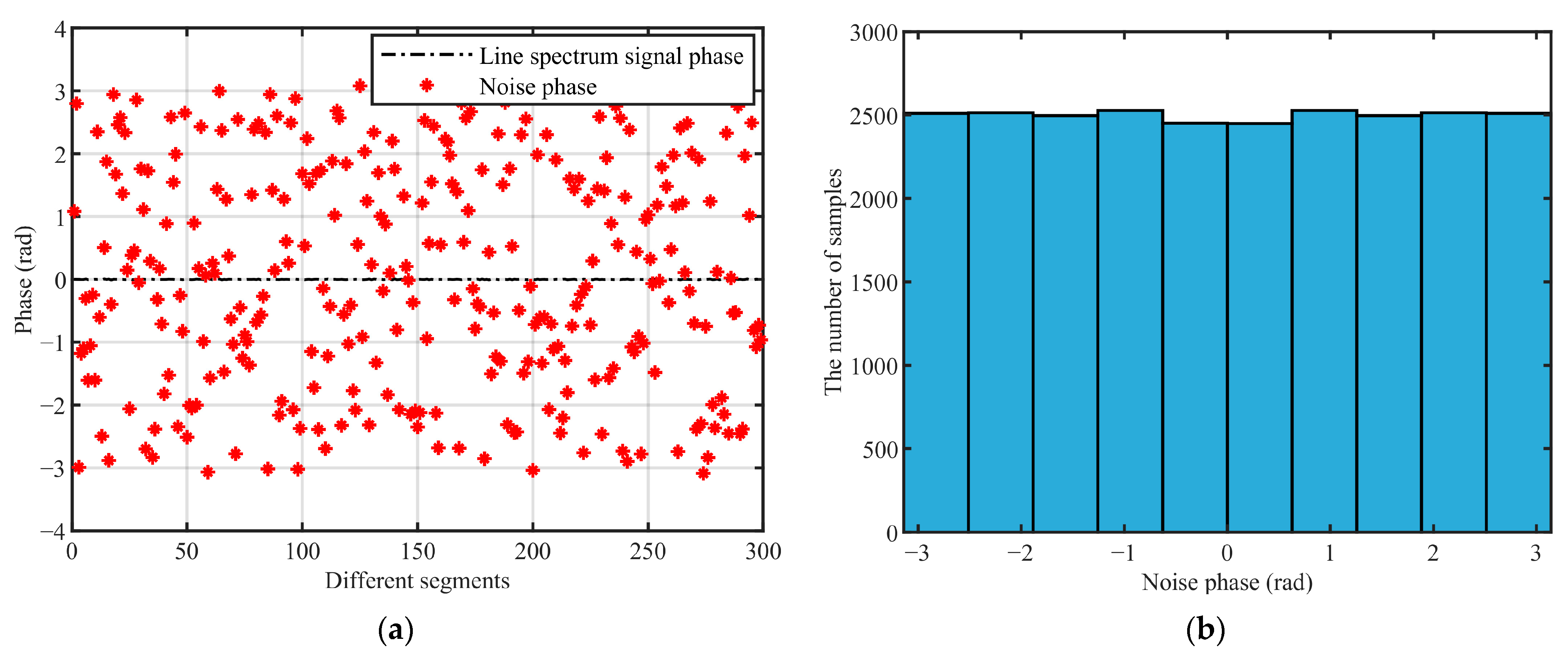
obtained from different segments will be constant, while the continuous spectrum noise will be incoherent; the phase of P N 1 m ω obtained from different segments will obey a uniform distribution of [ π , π ] . In the coherent averaging process, the line spectrum is unchanged, the noise is canceled, and the coherent gain is obtained (see Appendix A for the coherent averaging process).

3. Results

3.1. Simulation Data Analysis

3.1.1. Parameter Setting

To analyze the performance of the SHCS more intuitively, the effects of the input SNR (the SNR mentioned later in this paper are all in-band SNR; see Appendix B for the definition of in-band SNR), the number of averaging operations, and the overlap ratio (when the signal is segmented, the ratio of the same part of two adjacent segments to one segment is defined as the overlap rate) on the performance of the SHCS method under a background of Gaussian white noise were simulated. The ocean environment noise is approximately Gaussian [28] in some frequency bands, so in the simulation, Gaussian white noise can be used to simulate the ocean environment noise. In the simulations, a CW signal with the features of a line spectrum was transmitted; the frequency was 30 Hz and the sampling rate was 5 kHz. Firstly, in Section 3.1.2, the processing time (length of each segment) is T = 1 s, input SNR of 10, 1 dB was simulated. Then, in Section 3.1.3, the input SNR is 10 dB and the SHCS method performance of a different number of averaging operations was simulated. Finally, in Section 3.1.4, the input SNR is 10 dB and the SHCS method performance of different overlap ratios was simulated.

3.1.2. Effect of Input SNR

The performance of the SHCS method for processing the received signal was simulated, and the results were compared with the original power spectrum obtained by the Welch method. The calculation results are shown in Figure 2 and Figure 3.
According to the simulation results, the line-spectrum SNR on the original power spectrum obtained by the Welch method for the received signal is low. The SHCS method uses the coherence of the line spectrum and the non-coherence of the noise to obtain coherent gain, which improves the SNR of the line spectrum. Under a background of Gaussian white noise, the coherent gain is the difference between the line-spectrum coherence coefficient (in dB) and the noise coherence coefficient (in dB), which is consistent with the gain matrix G obtained in the theoretical derivation. As shown in Figure 2, under the conditions of 10 dB conventional input SNR (the line spectrum can be clearly observed on the original power spectrum), the coherence coefficient of the line spectrum decreases very little, and the noise coherence coefficient decreases by more than 10 dB; the SHCS method has excellent performance and can obtain a gain of about 13 dB. As shown in Figure 3, under the condition of an extremely low input SNR of 1 dB (the line spectrum is almost completely submerged by noise on the original power spectrum), the coherence coefficient of the line spectrum decreases by about 5 dB, and the coherence coefficient of the noise decreases by more than 10 dB. The SHCS still has good performance and a gain of about 8 dB can be obtained.
The offset m has basically no effect on the results of the SHCS method. When m = 1, the noise coherence coefficient drops to a minimum and continuing to increase m will not increase the gain. This is because the SHCS method divides the received signal into signal 1 and signal m, and signal m can be considered to be obtained after signal 1 is delayed by m. The CW signal is a stable periodic signal, so when m takes any values, the phase difference between signal 1 and signal m is constant, which shows that signal 1 and signal m have strong coherence and the coherence coefficient does not change with delay m. The background Gaussian white noise is a stationary random process; m takes any value and the noise phase difference between signal 1 and signal m changes randomly, which means that the noise in signal 1 and signal m is non-coherent, and the coherence coefficient is equal to Gaussian white noise coherence coefficient. Therefore, in this simulation, the coherence coefficient of the CW signal and the coherence coefficient of the noise have nothing to do with m, so the gain obtained by the SHCS method has nothing to do with m.

3.1.3. Effect of Number of Averaging Operations

From Equation (8), the SHCS method requires coherent averaging of the cross-power spectrum calculation results of each segment. In this section, to study the effect of the number of averaging operations on the SHCS, the performance of the SHCS method with different numbers of averaging operations was calculated in the case of m = 1. The calculation results are shown in Figure 4.
From Figure 4b, it can be seen that the coherence coefficient of the line spectrum does not change with the number of averaging operations and the noise coherence coefficient gradually decreases to its minimum value as the number of averaging operations increases. With an increasing number of averaging operations, the gain obtained by the SHCS method gradually increases and then tends to a stable value of around 15 dB. As shown in Appendix A, the SHCS gain comes from the coherent averaging process and is independent of the integration time T. From Figure 4c, it can be seen that when the number of averaging operations is fixed, the gains obtained using different integration durations T are basically the same. Under the condition that the total time of the received signal is constant, increasing the processing time T can increase the frequency resolution, but it also reduces the number of averaging operations. When the number of averaging operations has not reached the saturation value, reducing the number of averaging operations will reduce the gain obtained by the SHCS method. Therefore, the processing time T needs to be reasonably selected according to actual requirements.

3.1.4. Effect of Overlap Ratio

In the process of signal segmentation presented in Figure 1, to improve the number of averaging operations, a certain overlap ratio can be set. In this section, we simulate the effect of different overlap ratios on the performance of the SHCS method. The calculation results are shown in Figure 5.
From Figure 5a, it can be seen that the coherence coefficient of the line spectrum calculated by the SHCS method remains basically unchanged with the overlap ratio, while the noise coherence coefficient increases with the increase in overlap ratio. Figure 5b shows that the gain increases with the decrease in overlap ratio. When the offset m is 1, the SHCS process is as follows. The cross-power spectrum of the 1 to n and 2 to (n + 1) segments are taken and then coherently averaged. Because the added Gaussian white noise is a stationary random process, when the overlap ratio is 0, the corresponding two segments will also be stationary random processes, and the coherence coefficient will be very small. With an overlap ratio, some points of the two segments will become deterministic, so the coherence of the two segments will increase. The larger the overlap ratio, the stronger the noise coherence of the two segments and the smaller gain obtained by the SHCS method. In the extreme case, the overlap ratio is 1, and the (1 − n) segment will be cross-power spectrum averaged with itself. The coherence coefficient between the line spectrum and the noise will be 1, and the gain obtained by the SHCS will be 0.

3.2. Experimental Data Analysis

3.2.1. Experiment Description

To explore the performance of the SHCS method in an actual marine environment, an experiment was carried out in the Yellow Sea at a water depth of 46 m in the southeast of Shidao, Shandong Province. As shown in Figure 6, the receiving hydrophone was lowered into the sea to the side of the receiving ship and the transmitting ship carried the transmitting transducer gradually further from the receiving ship.
A schematic of the transmitting system is shown in Figure 7a and a schematic of the receiving system is shown in Figure 7b. In this experiment, a CW signal produced by the signal generator was sent to the transmitting transducer through the power amplifier. The signal received by the receiving hydrophone was stored in the computer through the signal collector.
The transmitting ship gradually moved away from the receiving ship, and when reaching a preset position, signals of different frequencies were transmitted. The receiving ship monitored and collected these signals using the receiving hydrophone. The positions of the transmitting and receiving ships, as obtained by Global Positioning System receivers, were recorded in real time.

3.2.2. Data Analysis

After completing the experiment, the received signals were processed by the SHCS method. The depth of the hydrophone was 12 m, the frequency of the transmitted signal was 190 Hz, the sampling rate was 5 kHz, the total signal time was 600 s, the processing time was T = 1 s, and the overlap ratio was 0. Firstly, the performance of the SHCS method under the conditions of a conventional input SNR were analyzed and the signals received at distances of 10 and 50 km were processed. The results are shown in Figure 8 and Figure 9.
From the calculation results, it can be seen that in an actual marine environment, coherence gain can be obtained by using the SHCS method to process the received signals. As shown in Figure 8 and Figure 9, when the overlap ratio is 0, m = 1, and T = 1 s, the SHCS method can obtain a gain of about 13 dB with a conventional input SNR. At the two receiving distances, an obvious spectrum peak can be observed on the original power spectrum. The SNR of the line spectrum can be greatly improved by using the SHCS, and the ease of line-spectrum extraction and subsequent detection is improved. This also increases the detection distance of a single hydrophone.
Next, the performance of the SHCS under the extremely low input SNR was analyzed; signals received at a distance of 100 km between the two ships were processed. The results are shown in Figure 10.
As shown in Figure 10, under the extremely low input SNR, almost no spectrum peak can be seen on the original power spectrum and it is impossible to use the single hydrophone to perform line-spectrum detection using the original power spectrum. After using the SHCS method, a coherence gain of about 10 dB is obtained, and the line spectrum can be clearly observed on the power spectrum after processing. As a result, the weak signal can be detected. The experimental processing results show that the ocean environmental noise coherence coefficient has been reduced to a minimum at m = 1, and continuing to increase m does not increase the gain obtained by the SHCS method. Therefore, it is sufficient to use the SHCS method to process the received signals in an actual marine environment using m = 1.
During the experiment, a cargo ship named Zhongsu 19 passed near to the receiving ship. This cargo ship was 189 m long, 32 m wide, and had a draft of 11 m. The radiated noise received by the single hydrophone was processed using the SHCS method and the results are shown in Figure 11.
From these results, it can be seen that after SHCS processing, the line spectrum of the cargo ship received by the single hydrophone is slightly reduced; the background noise is reduced by about 10 dB, and about 9 dB gain can be obtained when m = 1. As we all know, the ocean channel is time-varying and space-varying, it means that the same location receives different signals at different times, and different locations receive different signals at the same time. Generally, the ocean channel changes slowly with time, and in a relatively short time we can assume that the received signal does not much change. However, the ocean channel changes dramatically with spatial variation. For a stationary target, the received signal only introduces the time-varying feature of the ocean channel from the transmitting location to the receiving location. The transmitting location of the signal arriving at different times is the same, and the signal received at different times changes very little. It can be seen in Figure 8 that the coherence of the signal is basically unchanged over time. Figure 11 is the line spectrum of the radiation of a moving cargo ship processed by the SHCS method. Due to the movement of the cargo ship, the signal introduces time-varying and space-varying features of the ocean channel from the transmitting location to the receiving location, and the transmitting locations of the signals arriving at different times are different. The signal received at different times varies greatly, and the coherence of the signal decreases with time. At this time, the larger m is, the worse the coherence of the signal is and the smaller the gain. Therefore, it can be said that when dealing with actual moving ships, the SHCS method has the best performance when m = 1.

4. Discussion

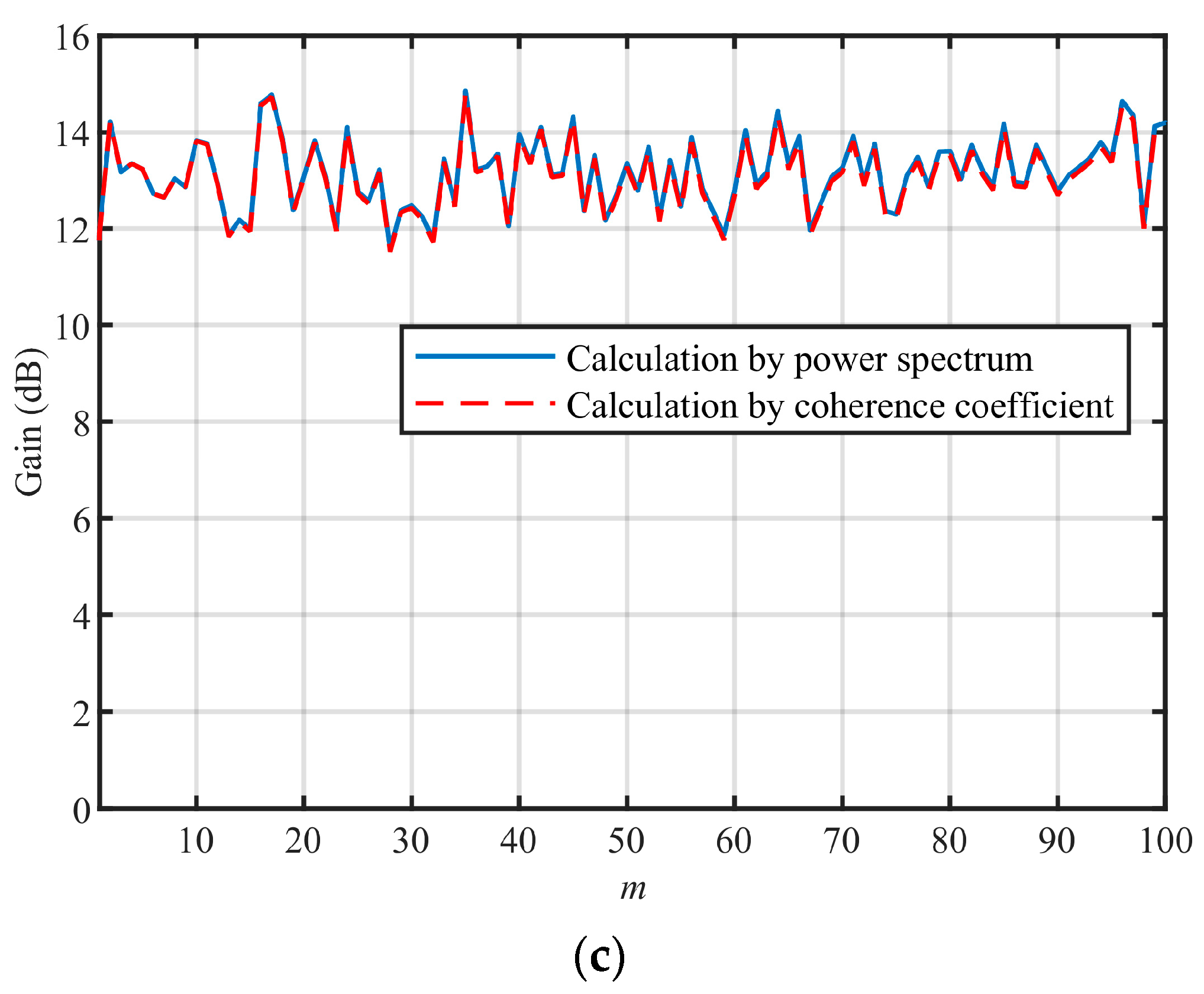
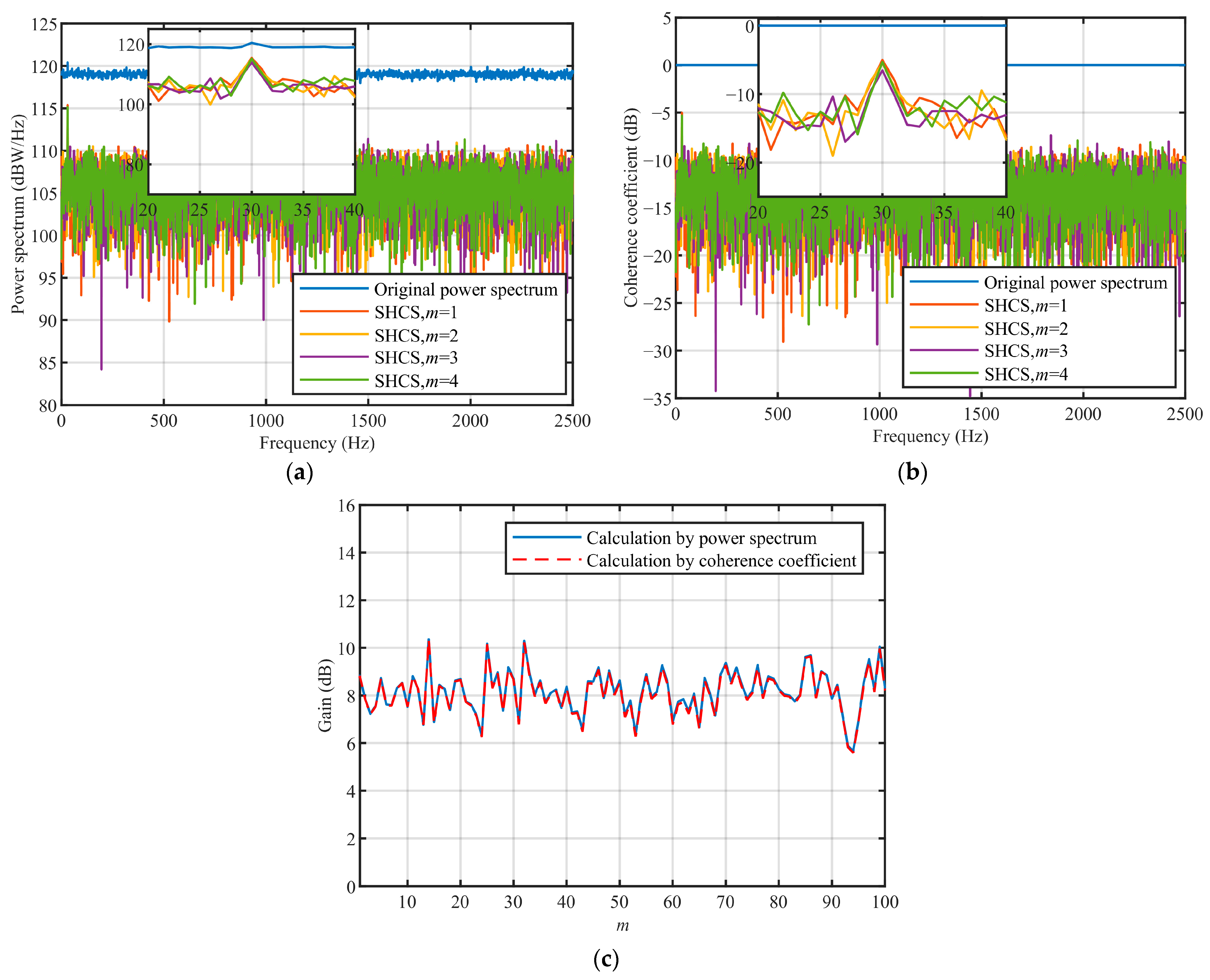
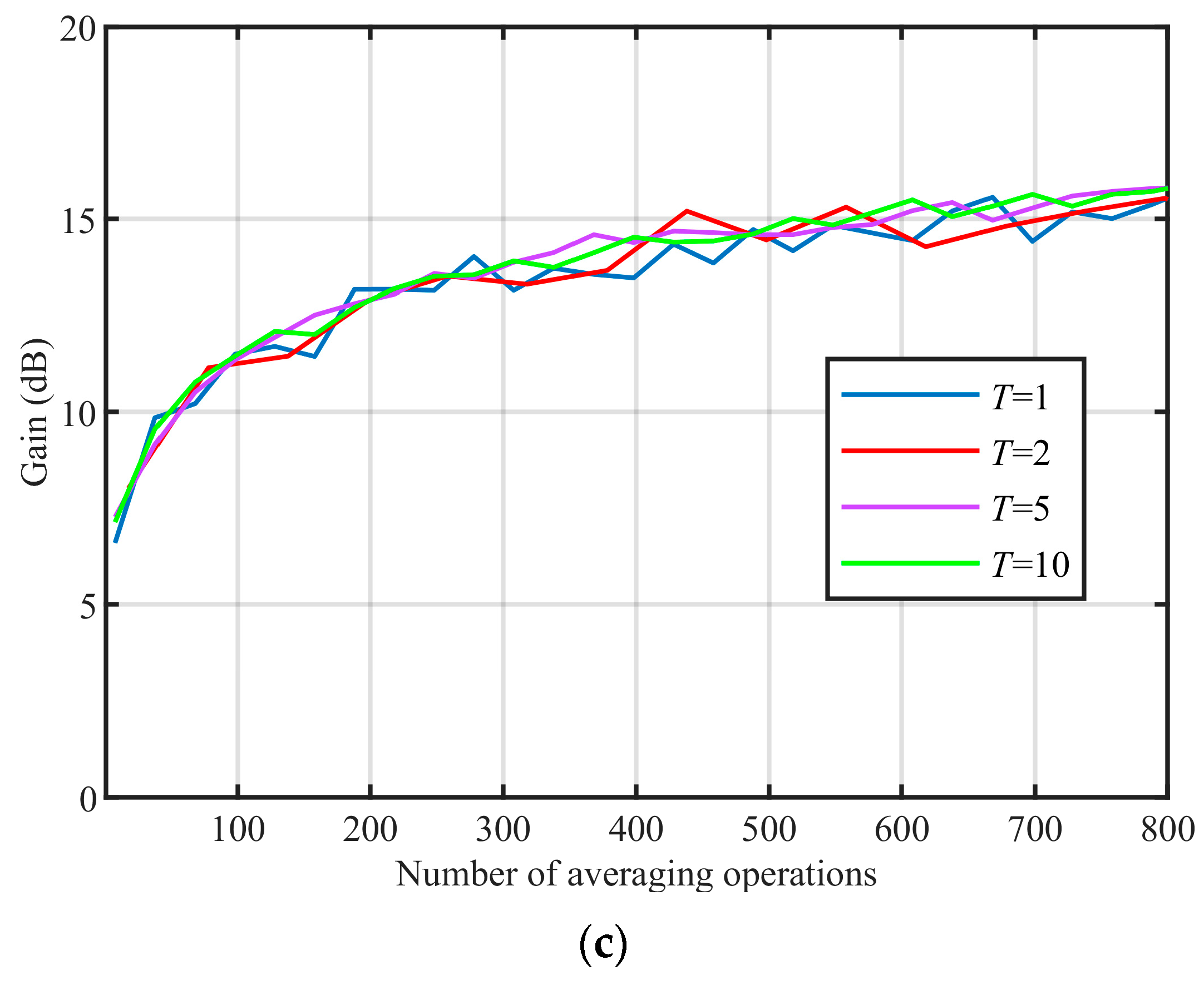
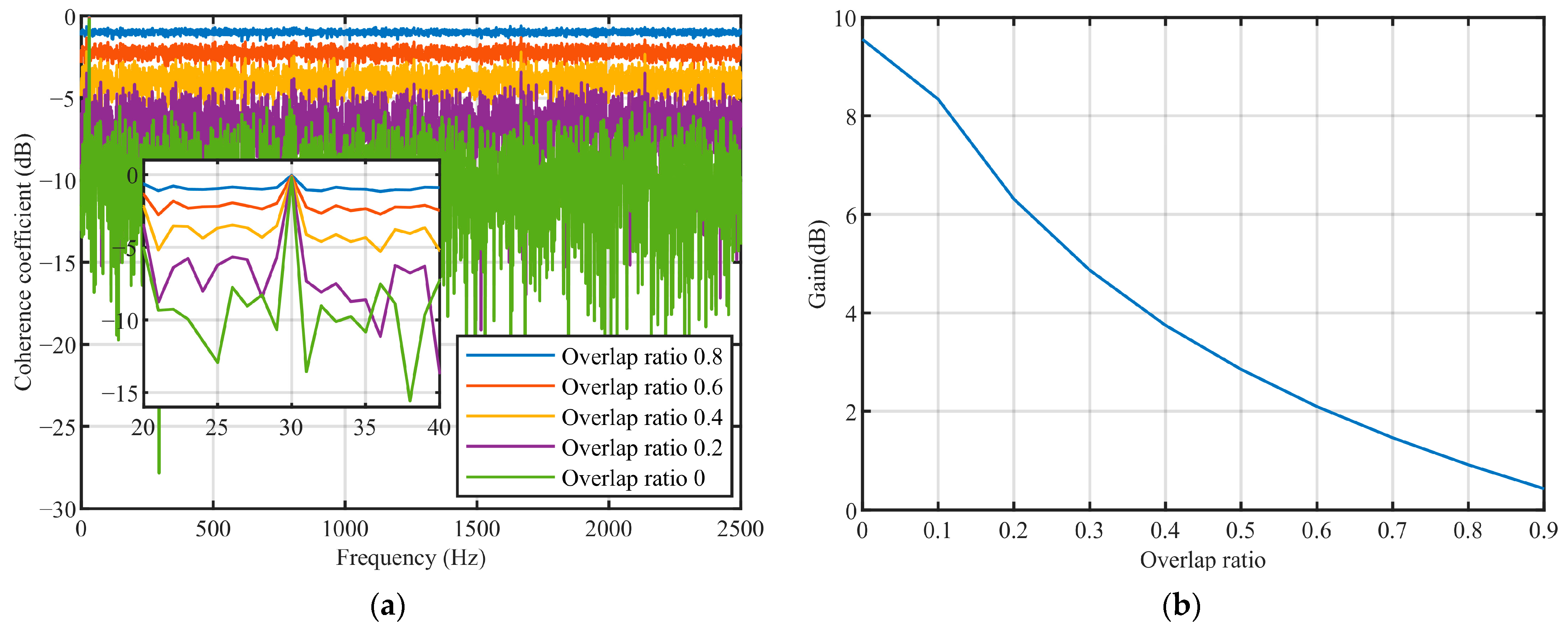
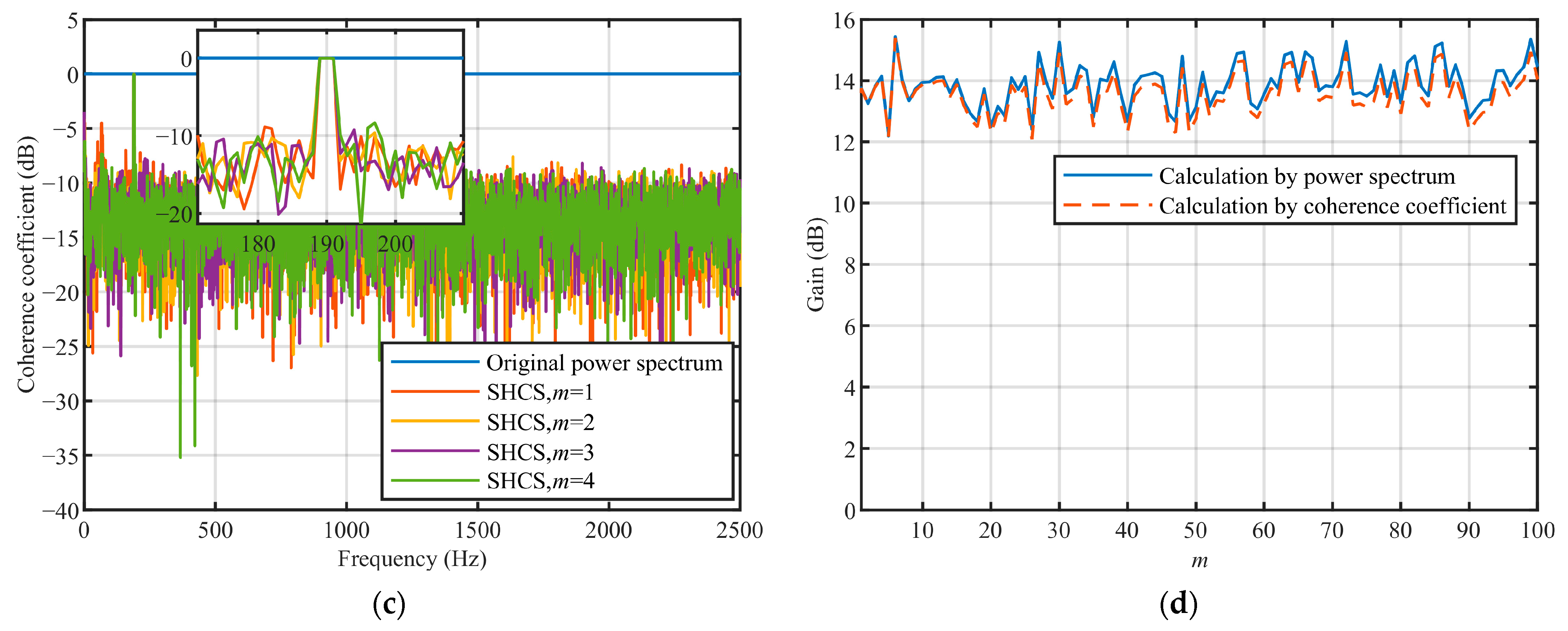
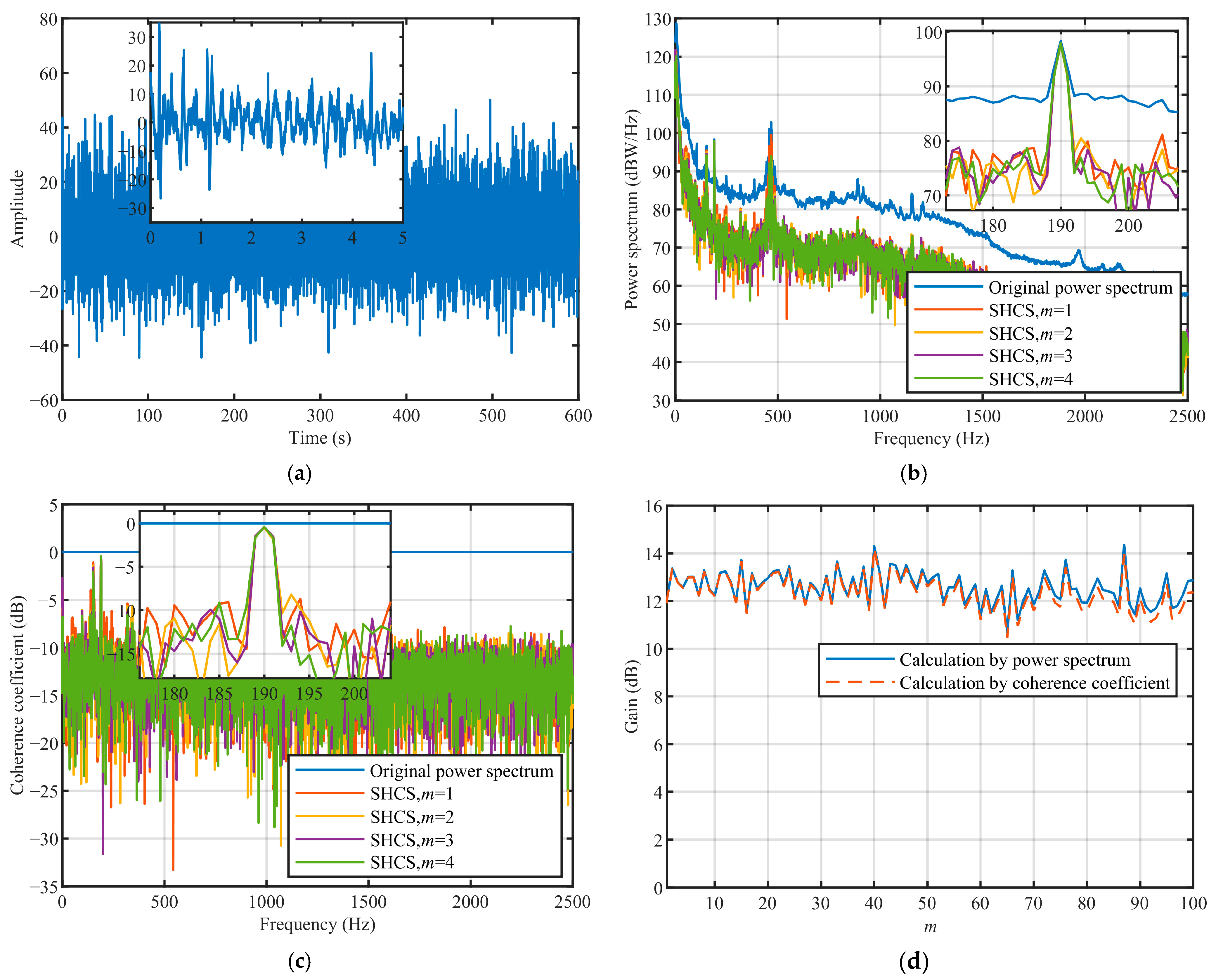
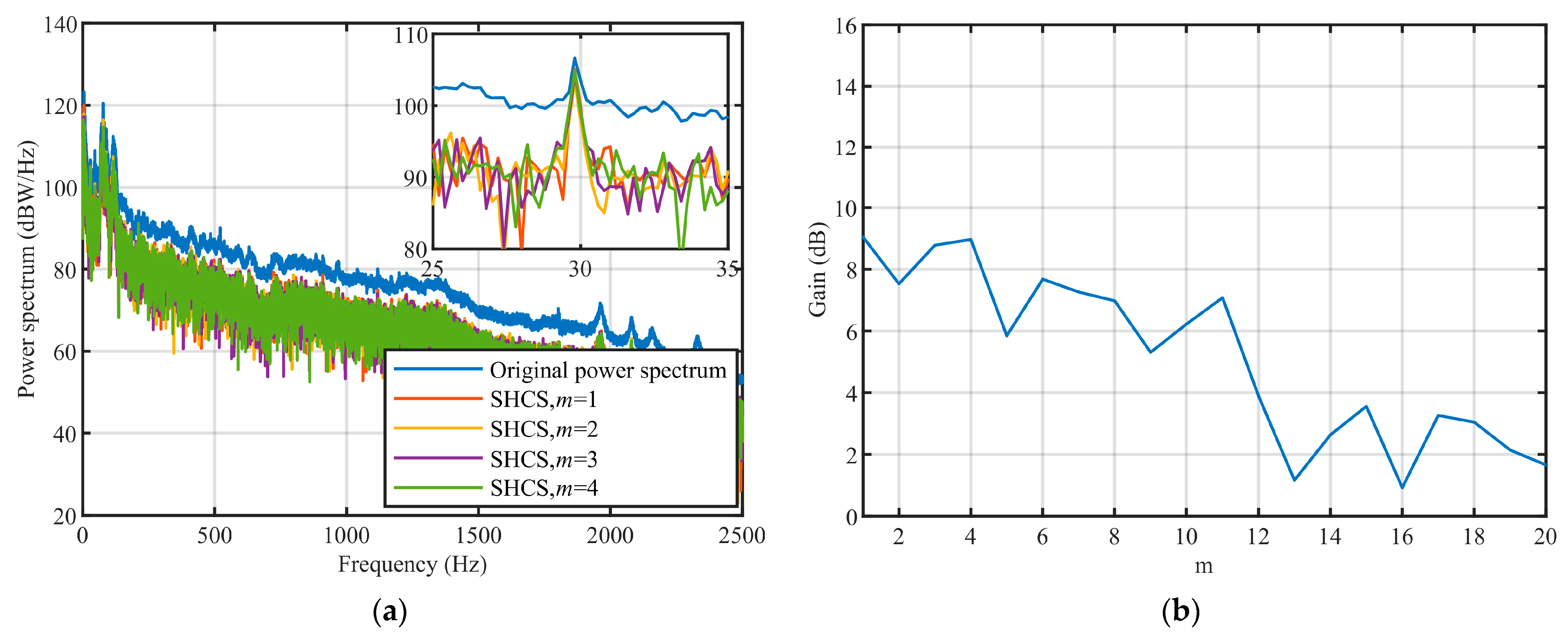
Simulation results show that the SHCS method has excellent performance under the different input SNR conditions. When the overlap ratio is 0 and m = 1, the noise coherence coefficient decreases to a minimum and no additional gain can be obtained by continuing to increase m. The gain obtained by the SHCS method increases with the increase in the number of averaging operations and gradually tends to a stable value. With the increase in overlap ratio, the coherence coefficient of the noise increases, the coherence coefficient of the line spectrum does not change, and the gain obtained by the SHCS method decreases.
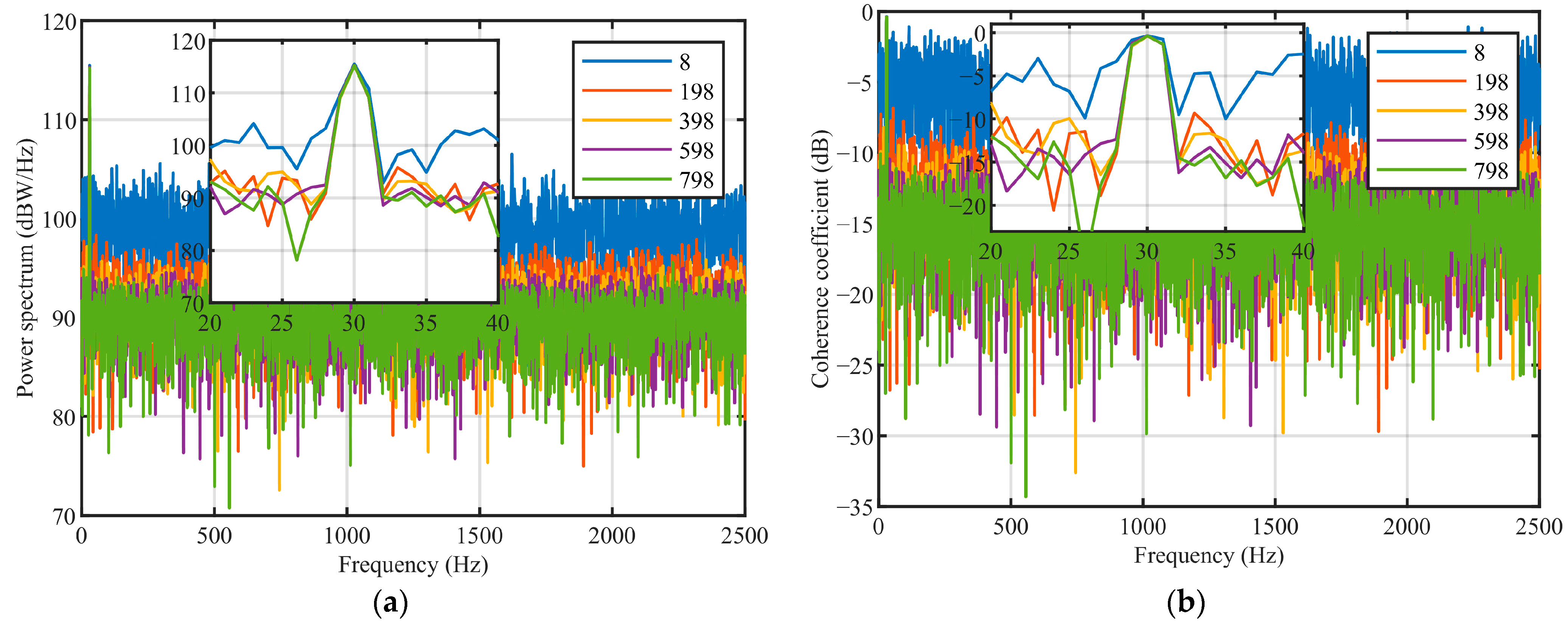
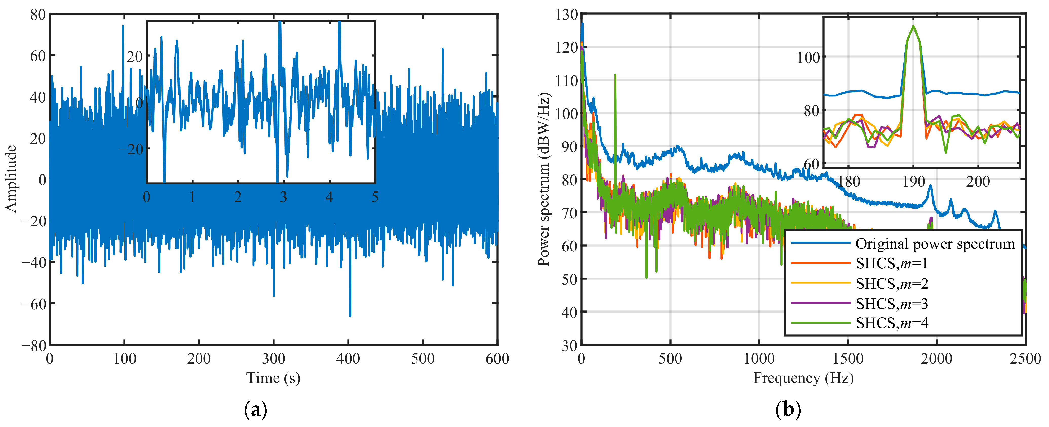
Experimental results show that the SHCS method has excellent performance in actual marine environments. Under the extremely low input SNR, in which the line spectrum was almost completely submerged in the marine environmental noise, the SHCS method was found to obtain a coherence gain of about 10 dB. Under the conventional input SNR, in which the line spectrum could be observed, the SHCS method was found to obtain a coherence gain of about 13 dB. The results of processing the radiated noise from an actual cargo ship also demonstrate the effectiveness of the SHCS method.
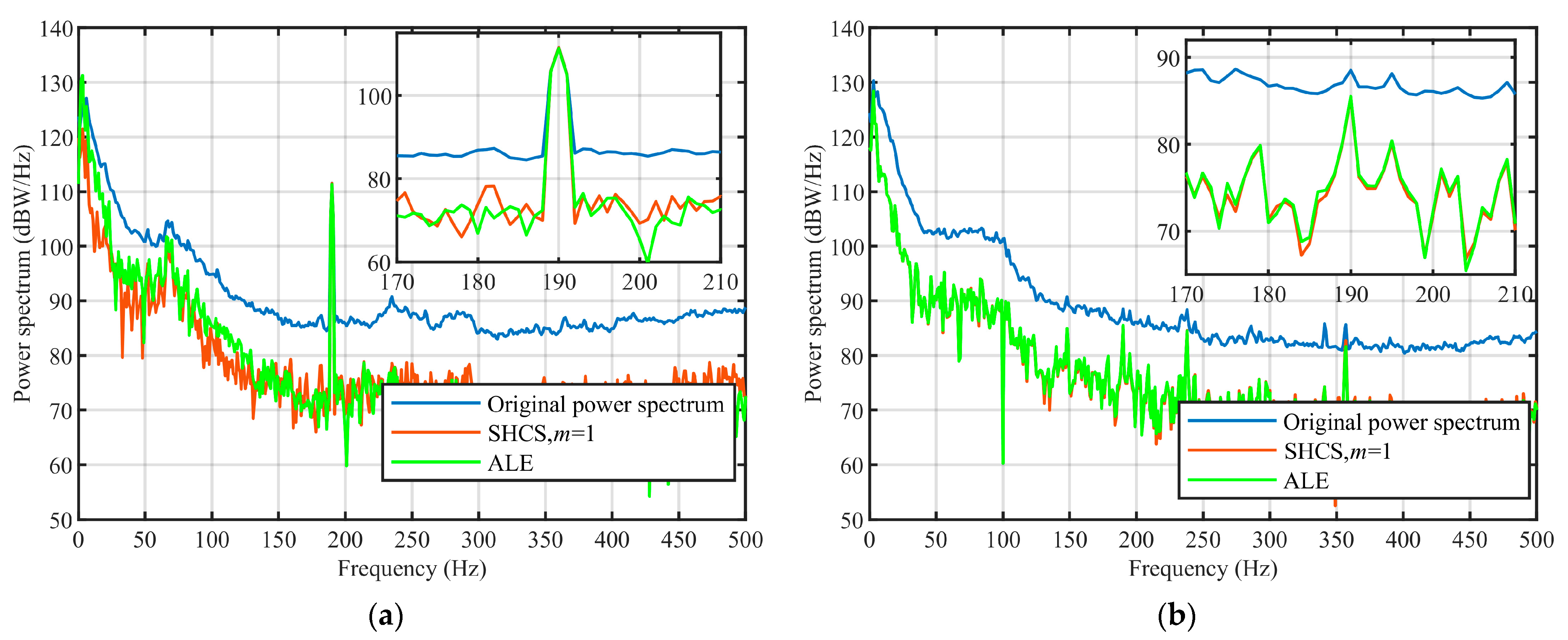
Our study shows that the SHCS method has excellent performance and can significantly improve the SNR of weak line spectrum. The SHCS method improves the line spectrum SNR through the coherence of the signal and the non-coherence of the noise, which is essentially different from the background equalization and ALE method. The background equalization technology [15,16,17,18] is based on the difference between the signal and the noise amplitude. This technology sets an appropriate threshold, filters the signal, and filters out the background noise and protects the signal. However, at low SNR, where the signal is almost buried in the noise, background equalization techniques usually work poorly. The ALE method [22,23,24,25,26,27] is an essentially adaptive filter that enhances the signal by self-adjusting the errors between the desired signal and the output signal, but the method converges slowly under low SNR. Moreover, when there are multiple line spectra in the frequency spectrum, the enhancement range of the weak line spectrum is smaller than that of the strong line spectrum. Next, the SHCS method and ALE method were used to process experimental data, respectively, and the results are shown in 
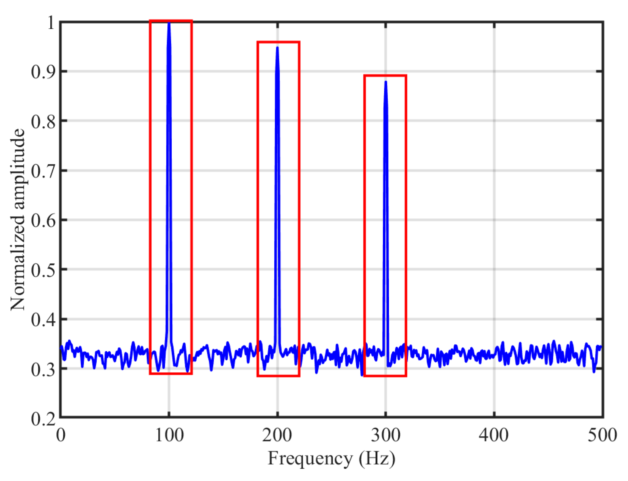
Figure 12. The results show that the SHCS method, as a new method, can achieve roughly the same gain as the ALE method and can significantly improve the line spectrum SNR. Compared with the ALE method, the SHCS method has its own advantages. It can quickly process signals with different SNR when there are multiple line spectra in the power spectrum and after SHCS processing, the strong and weak line spectrum obtained basically same gains.
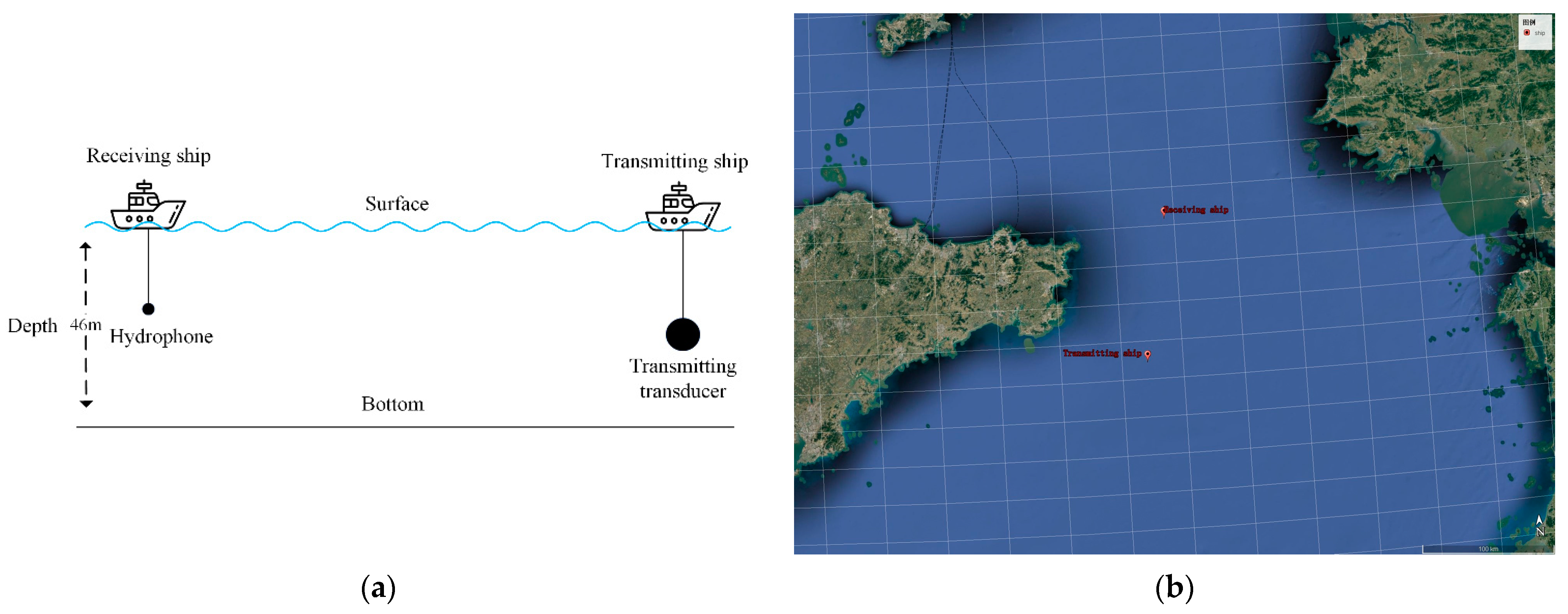
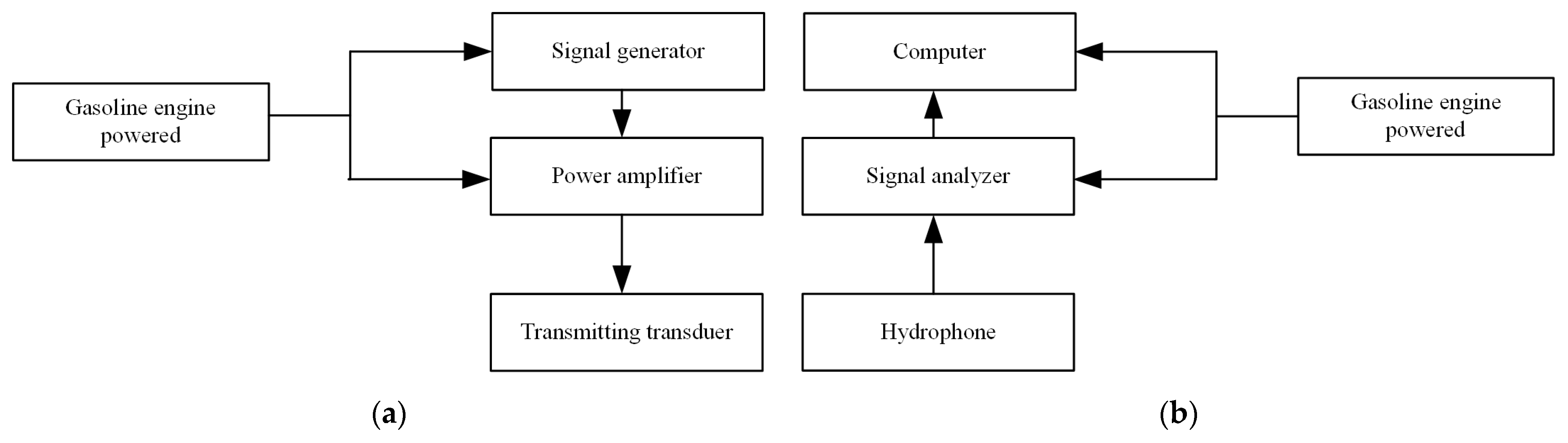
After SHCS processing, the detection range of passive sonar is improved and this increases the ability of small-sized platforms to observe surface ships and underwater submarines in the ocean at long distances. The SHCS method is suitable for observing not only radiated ship noise but also any signals with line-spectrum characteristics. In future work, we hope to use the SHCS method to observe other industrial activities in the ocean, and we hope that it can be applied to a vector hydrophone.

5. Conclusions

To improve the line-spectrum detection ability of a single hydrophone, we propose the SHCS method to obtain coherence gain and improve the SNR of the line spectrum based on the coherence of the line spectrum and the non-coherence of the noise. The effects of input SNR, number of averaging operations, and overlap ratio on the performance of the SHCS method under a background of Gaussian white noise were simulated. The simulation results showed that when the overlap ratio is 0, the SHCS can achieve the best performance when the number of averaging operations reaches saturation, and about 15 dB coherence gain can be obtained. Finally, we used the SHCS method to process a CW signal in an actual marine environment. The experimental results showed that the SHCS method has excellent performance in an actual marine environment, and it greatly improves the line-spectrum detection capability of a single hydrophone. Under the extremely low input SNR, when the spectrum peak is almost completely submerged in the marine environmental noise, about 10 dB gain can be obtained by using the SHCS method to process the weak signal in an actual marine environment. The results obtained from processing the noise radiated from an actual cargo ship also demonstrate the effectiveness of the SHCS method.

Author Contributions

Z.Z.: Writing—Original Draft, Methodology, Formal Analysis. Q.L.: Conceptualization, Project administration. Z.X.: Funding Acquisition, Writing—Review & Editing. D.S.: Writing—Review & Editing. All authors have read and agreed to the published version of the manuscript.

Funding

This research was supported by the National Natural Science Foundation of China (Grant No. 62171148).

Data Availability Statement

The data presented in this paper are available after contacting the corresponding author.

Conflicts of Interest

The authors declare that the research was conducted in the absence of any commercial or financial relationships that could be construed as a potential conflict of interest.

Appendix A. Coherent Averaging Process

According to Equation (8), for the two-channel signal segmented in Figure 1, the SHCS method needs to obtain the cross-power spectrum of the corresponding segment and then performs coherent averaging. Assuming that the lengths of signal 1 and signal m are 300 s and the processing time is T = 1 s, they are each divided into 300 segments. The 300 cross-power spectra of the corresponding segments are then calculated along with their phases, and the variation of the phases of the line spectrum and the noise can be plotted with respect to the segment, as shown in Figure A1a.
It can be found that the phase of the line spectrum does not change with the segment, and it will thus not be canceled during the coherent averaging; the noise phase, however, varies randomly. A histogram of the noise phase on the cross-power spectrum is plotted in Figure A1b. It can be seen that this obeys a uniform distribution of [ π , π ] , so the noise will be coherently canceled during the coherent averaging process. After coherent averaging, the level of the line spectrum on the power spectrum remains unchanged, but the level of the noise spectrum decreases due to coherent cancellation, thereby improving the SNR of the line spectrum on the power spectrum.
Figure A1. Phase distribution on the power spectrum: (a) phase variation with segment; (b) noise phase histogram.
Remotesensing 15 00659 g0a1

Appendix B. In-Band SNR

In line-spectrum detection, the in-band SNR is usually used to describe the relative magnitude of the line spectrum and the continuum spectrum noise. The in-band SNR is defined as the ratio of the power at a line-spectrum frequency point to the average power of the noise within a certain bandwidth. The calculation method is shown in Figure A2. The noise is additive white Gaussian noise, and only the frequency point at which the line spectrum peak is located is selected; then, noise frequency points within a certain bandwidth around this are used to calculate the in-band SNR. The red boxes in Figure A2 show the range of the frequency points selected to calculate the in-band SNR. The in-band SNR equation is:
SNR = P s f 0 P ¯ n
where P n f is the power of the noise on the power spectrum, P ¯ n = B P n f B is the average power of the noise within a certain bandwidth B, and P s f 0 is the power at the line-spectrum frequency point on the power spectrum.
Figure A2. Schematic diagram of the calculation method for the in-band SNR.
Remotesensing 15 00659 g0a2

References

  1. Hildebrand, J.A. Anthropogenic and natural sources of ambient noise in the ocean. Mar. Ecol. Prog. Ser. 2009, 395, 5–20. [Google Scholar] [CrossRef] [Green Version]
  2. Hu, G.; Wang, K.; Liu, L. Detection line spectrum of ship radiated noise based on a new 3D chaotic system. Sensors 2021, 21, 1610. [Google Scholar] [CrossRef] [PubMed]
  3. Nielsen, R.O. Sonar Signal Processing; Artech House, Inc.: Norwood, MA, USA, 1991. [Google Scholar]
  4. Waite, A.D. Sonar for Practising Engineers, 3rd ed.; Wiley: Hoboken, NJ, USA, 2002. [Google Scholar]
  5. Hodges, R.P. Underwater Acoustics: Analysis, Design and Performance of Sonar; John Wiley & Sons: Hoboken, NJ, USA, 2011. [Google Scholar]
  6. Marage, J.-P.; Mori, Y. Sonar and Underwater Acoustics; John Wiley & Sons: Hoboken, NJ, USA, 2013. [Google Scholar]
  7. Cooley, J.W.; Tukey, J.W. An algorithm for the machine calculation of complex Fourier series. Math. Comput. 1965, 19, 297–301. [Google Scholar] [CrossRef]
  8. Rosenlicht, M. Introduction to Spectral Analysis; Dover Publications: New York, NY, USA, 2005. [Google Scholar]
  9. Burenkov, S.V.; Gavrilov, A.N.; Uporin, A.Y.; Furduev, A.V. Heard Island Feasibility Test: Long-range sound transmission from Heard Island to Krylov underwater mountain. J. Acoust. Soc. Am. 1994, 96, 2458–2463. [Google Scholar] [CrossRef]
  10. Li, Q. Digital Sonar Design in Underwater Acoustics; Zhejiang University Press: Zhejiang, China, 2012. [Google Scholar]
  11. Rao, B.D.; Hari, K.V.S. Weighted subspace methods and spatial smoothing: Analysis and comparison. IEEE Trans. Signal Process. 1993, 41, 788–803. [Google Scholar] [CrossRef] [Green Version]
  12. Qian, C. A simple modification of ESPRIT. IEEE Signal Process. Lett. 2018, 25, 1256–1260. [Google Scholar] [CrossRef]
  13. Bartlett, M.S. Smoothing periodograms from time-series with continuous spectra. Nature 1948, 161, 686–687. [Google Scholar] [CrossRef]
  14. Welch, P. The use of fast Fourier transform for the estimation of power spectra: A method based on time averaging over short, modified periodograms. IEEE Trans. Audio Electroacoust. 1967, 15, 70–73. [Google Scholar] [CrossRef] [Green Version]
  15. Struzinski, W.A.; Lowe, E.D. A performance comparison of four noise background normalization schemes proposed for signal detection systems. J. Acoust. Soc. Am. 1984, 76, 1738–1742. [Google Scholar] [CrossRef]
  16. Stergiopoulos, S. Noise normalization technique for beamformed towed array data. J. Acoust. Soc. Am. 1995, 97, 2334–2345. [Google Scholar] [CrossRef]
  17. Filho, W.S.; de Seixas, J.M.; de Moura, N.N. Preprocessing passive sonar signals for neural classification. IET Radar Sonar Navig. 2011, 5, 605–612. [Google Scholar] [CrossRef]
  18. Kuhn, J.P.; Heath, T.S. Apparatus for and Method of Adaptively Processing Sonar Data. U.S. Patent No 5,481,503; U.S. Patent and Trademark Office: Washington, DC, USA, 2 January 1996. [Google Scholar]
  19. Bentrem, F.W.; Botts, J.; Summers, J.E. Design of a signal normalizer for high-clutter active-sonar detection. J. Acoust. Soc. Am. 2018, 143, 1760. [Google Scholar] [CrossRef]
  20. Wang, C.; Zhu, G.P.; Yin, J.W.; Guo, L.X.; Zhang, Y.Z. Experimental study of passive detection of underwater targets across ice. Appl. Acoust. 2022, 191, 108672. [Google Scholar] [CrossRef]
  21. Zhang, J.; Li, Y.A.; Ali, W.; Liu, L. Line spectrum enhancement of underwater acoustic signals using Kalman filter. J. Marine Sci. Appl. 2020, 19, 148–154. [Google Scholar] [CrossRef]
  22. Hollmann, L.J.; Stevenson, R.L. Adaptive whitening of ambient ocean noise with narrowband signal preservation. J. Acoust. Soc. Am. 2016, 139, 3122–3133. [Google Scholar] [CrossRef] [PubMed]
  23. Haykin, S.S. Adaptive Filter Theory; Pearson Education: Noida, India, 2022. [Google Scholar]
  24. Haykin, S. The LMS filter algorithm. In Least-Mean-Square Adaptive Filters; Haykin, S., Widrow, B., Eds.; Wiley: New York, NY, USA, 2003. [Google Scholar]
  25. Campbell Jr, R.L.; Younan, N.H.; Gu, J. Performance analysis of the adaptive line enhancer with multiple sinusoids in noisy environment. Signal Process. 2002, 82, 93–101. [Google Scholar] [CrossRef]
  26. Liang, G.L.; Hao, Y.; Zou, N.; Qiu, L.H. Sparsity-based frequency-domain adaptive line enhancer. J. Acoust. Soc. Am. 2019, 146, 2799. [Google Scholar] [CrossRef]
  27. Hao, Y.; Qiu, L.; Chi, C.; Liang, G.L. Sparsity-inducing frequency-domain adaptive line enhancer for unmanned underwater vehicle sonar. Appl. Acoust. 2021, 173, 107689. [Google Scholar] [CrossRef]
  28. Carey, W.M.; Evans, R.B. Ocean Ambient Noise: Measurement and Theory; Springer Science and Business Media: Berlin, Germany, 2011. [Google Scholar]
Figure 1. Schematic diagram of SHCS method.
Remotesensing 15 00659 g001
Figure 2. SHCS processing results with input SNR = 10 dB: (a) power-spectrum estimation (re 0.67 × 10⁻¹⁸ W/Hz); (b) coherence-coefficient calculation results; (c) gain.
Remotesensing 15 00659 g002aRemotesensing 15 00659 g002b
Figure 3. SHCS processing results with input SNR = 1 dB: (a) power-spectrum estimation; (b) coherence-coefficient calculation results; (c) gain.
Remotesensing 15 00659 g003
Figure 4. SHCS processing results with different numbers of averaging operations: (a) power-spectrum estimation with T = 1 s; (b) coherence-coefficient calculation with T = 1 s; (c) gain.
Remotesensing 15 00659 g004aRemotesensing 15 00659 g004b
Figure 5. SHCS processing results with different overlap ratios: (a) coherence coefficient; (b) gain.
Remotesensing 15 00659 g005
Figure 6. Schematic diagram of the sea experiments: (a) layout diagram; (b) satellite image.
Remotesensing 15 00659 g006
Figure 7. Schematics of experimental equipment: (a) transmitting system, (b) receiving system.
Remotesensing 15 00659 g007
Figure 8. SHCS processing results at 10 km with different values of m: (a) time domain waveform; (b) power-spectrum estimation; (c) coherence coefficient; (d) gain.
Remotesensing 15 00659 g008aRemotesensing 15 00659 g008b
Figure 9. SHCS processing results at 50 km with different values of m: (a) time domain waveform; (b) power-spectrum estimation; (c) coherence coefficient; (d) gain.
Remotesensing 15 00659 g009
Figure 10. SHCS processing results at 100 km with different values of m: (a) time domain waveform; (b) power-spectrum estimation; (c) coherence coefficient; (d) gain.
Remotesensing 15 00659 g010
Figure 11. SHCS processing results for the Zhongsu 19 radiated noise: (a) power-spectrum estimation; (b) gain.
Remotesensing 15 00659 g011
Figure 12. SHCS method compared with ALE method: (a) 10 km; (b) 100 km.
Remotesensing 15 00659 g012
Disclaimer/Publisher’s Note: The statements, opinions and data contained in all publications are solely those of the individual author(s) and contributor(s) and not of MDPI and/or the editor(s). MDPI and/or the editor(s) disclaim responsibility for any injury to people or property resulting from any ideas, methods, instructions or products referred to in the content.

