Article

A Traffic-Aware Fair MAC Protocol for Layered Data Collection Oriented Underwater Acoustic Sensor Networks

School of Electrical and Information Engineering, Tianjin University, Tianjin 300072, China
*
Author to whom correspondence should be addressed.
Remote Sens. 2023, 15(6), 1501; https://doi.org/10.3390/rs15061501
Submission received: 2 February 2023 / Revised: 3 March 2023 / Accepted: 6 March 2023 / Published: 8 March 2023
(This article belongs to the Special Issue Underwater Communication and Networking)

Abstract

:
Underwater acoustic channels are characterized by long propagation delay, limited available bandwidth and high energy costs. These unique characteristics bring challenges to design media access control (MAC) protocol for underwater acoustic sensor networks (UASNs). Especially in data-collection-oriented UASNs, data generated at underwater nodes are transmitted hop-by-hop to the sink node. The traffic loads undertaken by nodes of different depths are different. However, most existing MAC protocols do not consider the traffic load imbalance in data-collection-oriented UASNs, resulting in unfairness in how the nodes transmit their own generated data. In this paper, we propose a novel traffic-aware fair MAC protocol for layered data-collection-oriented UASNs, called TF-MAC. TF-MAC accesses a medium by assigning time slots of different lengths to each layer via different traffic loads to achieve traffic fairness of nodes. To improve throughput and avoid collision in the network, an overlapping time slot division mechanism for different layers and multi-channel allocation scheme within each single layer is employed. Considering the time-varying traffic loads of the nodes, an adaptive packet length algorithm is proposed by taking advantage of the spatial-temporal uncertainty of underwater channels. A sea experiment was conducted to prove the spatial-temporal uncertainty of UASNs, which provides a feasibility basis for the proposed algorithm. Simulation results show that TF-MAC can greatly improve the network performance in terms of throughput, delay, energy consumption, and fairness in the layered data-collection-oriented UASNs.

1. Introduction

Underwater acoustic sensor networks (UASNs) have been widely used in oceanography data collection, ocean surveillance and disaster warning [1,2,3]. Data-collection-oriented UASNs, which are used for sampling high-precision underwater information, have attracted significant interest in recent years [4].
However, UASNs must confront many challenges to become a promising technique. Because electromagnetic signals do not work well due to their rapid attenuation in water, acoustic communication is a superior method for long-distance underwater communication [5]. Compared with radio signals, acoustic signals are subject to long and variable propagation delay, limited bandwidth, and high energy costs [6,7,8]. These special characteristics pose great challenges for protocol design in UASNs.
The media access control (MAC) protocol solves the problem of multi-user channel sharing and avoiding packet collisions. Due to high delay and high transmission power costs, underwater collision can severely reduce throughput and increase power consumption. Hence, some existing MAC protocols have been proposed [9,10], in which the sink node arranges collision-free scheduling for all nodes. One drawback of these protocols is that they were originally designed for single-hop networks. However, due to the limits on acoustic transmission range, a single-hop network cannot cover a large area. Therefore, the data-collection-oriented UASNs are usually multi-hop networks, in which the data generated at the sensor nodes are transmitted to the sink node hop-by-hop. An interference-aware data transmission protocol named the cellular clustering-based interference-aware data transmission protocol (CIDP) is proposed in [11]. This protocol employs a time division multiple access (TDMA) scheduling scheme to reduce interference and a layered routing scheme to achieve reliable data transmission in UASNs. Although this MAC significantly reduces interference in a multi-hop network, the relay nodes that are deployed are dedicated solely to packet forwarding, which is a waste of node resources.
A data-collection-oriented UASN consists of a sink node and many sensor nodes. All sensor nodes transmit the collected data in the direction of the sink node. The directional transmission of packets may lead to the traffic load in the network becoming non-uniformly distributed. That is, the closer to the sink node, the more data are handled by the sensor node. This will result in unfairness in how nodes at different depths send their own generated data. However, most existing MAC protocols do not consider the depth-based load imbalance in UASNs. The depth-based routing MAC (DBR-MAC) [12] introduced a depth-based scheme into the design of UASNs for the first time. It adopted a depth-scheduling algorithm to give priority to key nodes in the conflicting domain to access the channel. However, due to the long-delay hidden terminal problem, it cannot avoid conflicts by listening to the transmissions of neighbors.
In UASNs, the traffic load in each node exhibits dynamic characteristics [13]. Therefore, it is necessary to consider the time-varying traffic load to improve the adaptability of the MAC. One possible method is to construct a new schedule tailored to the new traffic pattern whenever the traffic load changes. However, identifying new traffic patterns and broadcasting a new schedule over the network require both sensor nodes to communicate with each other, which introduces extra energy and delay, particularly when the traffic load changes frequently. Another way to adapt to dynamic traffic load is to use hybrid protocols. The underwater practical MAC (UPMAC) [13] attempts to be adaptive to the network load conditions by providing two modes and switching between them based on different loads being offered. The hybrid MAC protocols achieve good performance in single-hop networks. However, when these hybrid MAC protocols are extended to multi-hop networks, it is possible for a node to execute multiple protocols simultaneously, which can cause transmission conflicts. Therefore, it is desirable to propose an effective method to adapt to the traffic dynamics in the network.
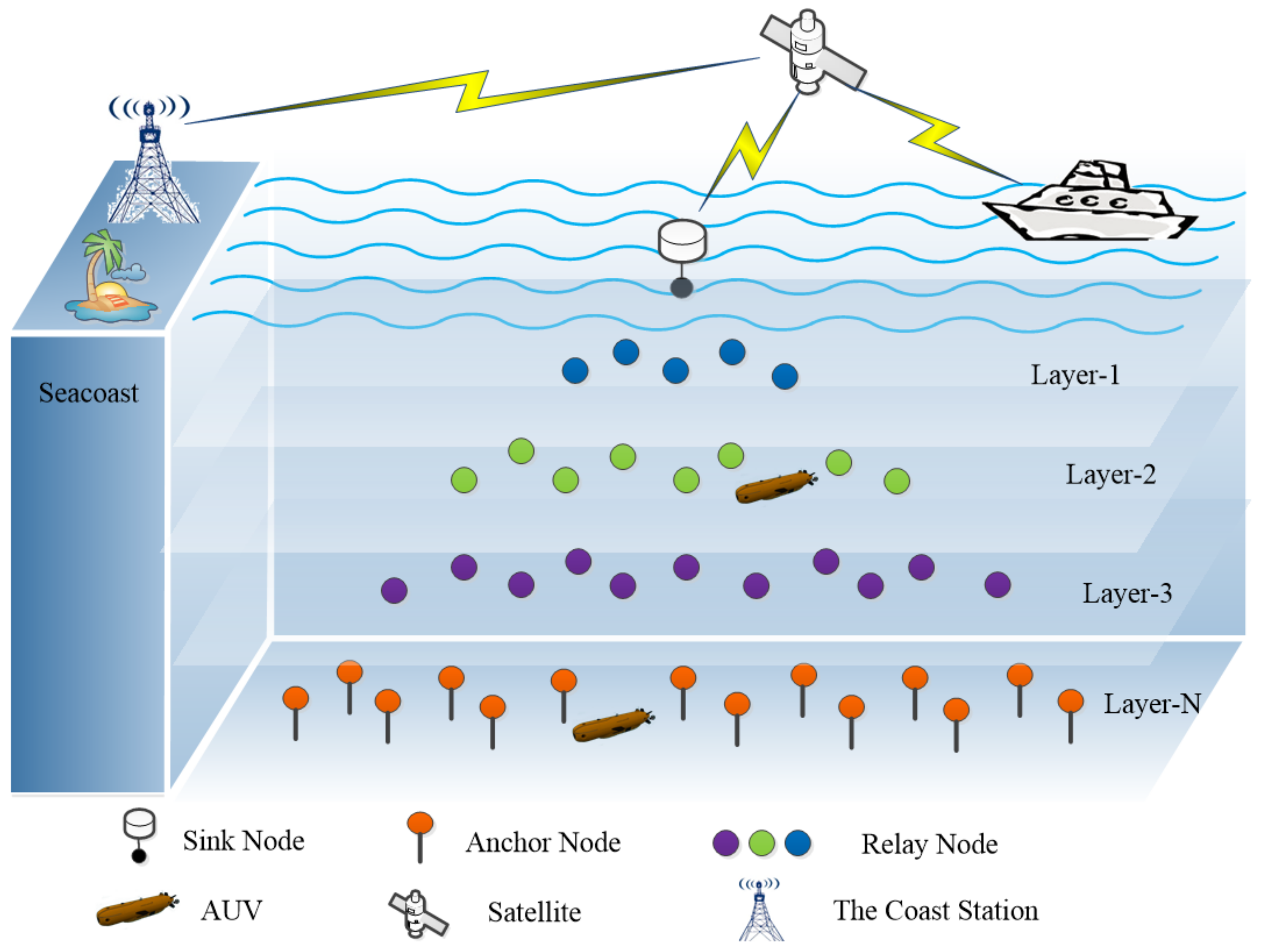
To address the issues mentioned above, we propose a traffic-aware fair MAC protocol (TF-MAC) for data-collection-oriented UASNs. In this paper, we consider a layered data-collection-oriented UASN with a tree topology, in which nodes of different depths represent different layers. In TF-MAC, the sink node employs a TDMA scheme to schedule the time slots for the nodes of each layer. This is performed to avoid the possibility of vertical collision occurring between nodes located in adjacent layers. To avoid horizontal conflict that may occur when the nodes of the same layer are transmitting to the nodes of the upper layer, a multi-channel mechanism is adopted. Therefore, TF-MAC ensures collision-free transmissions and receptions of DATA packets.
The main contributions of this paper can be summarized as follows:
  • In order to improve fairness, we allocate different time slot lengths for each layer. An overlapping time slot division mechanism is employed. This mechanism allows layers that are two layers away from each other to communicate in parallel without interfering.
  • TF-MAC allocates the subchannel to the underwater nodes based on the protocol interference model. Then, power control is carried out for each node based on the physical interference model, which ensures no interference while reducing energy consumption.
  • To improve performance in traffic load time-varying situations, we design an adaptive packet length algorithm based on the spatial-temporal uncertainty of underwater channels. Each node is aware of traffic load changes to adaptively update packet length, which is not achieved in other MAC protocols.
The remainder of this paper is organized as follows. In Section 2, we introduce the related work. Section 3 introduces the system model. In Section 4, the TF-MAC protocol is described in detail. In Section 5, we present a sea experiment to verify the spatial-temporal uncertainty. In Section 6, the simulation results are shown and discussed. Finally, we conclude this paper in Section 7.

2. Related Work

There has been intensive design of traffic aware and fair MAC protocols for terrestrial sensor networks. The rate-based Fair-Aware Congestion Control (FACC) [14] protocol can control congestion and achieve an approximately fair bandwidth allocation for different flows. The rate-aware congestion control (RACC) [15] protocol improves congestion by establishing congestion levels and source rate regulation. However, due to the high energy consumption and high propagation delay of UASNs, the techniques currently developed on terrestrial sensor networks are not applicable to the acoustic communication medium of UASNs.
In the past decades, many MAC protocols have been proposed for UASNs, which can be classified into two categories: contention-based and contention-free [16]. In contention-based protocols, nodes access the channel at random. In the contention-free protocol, the nodes access the channel according to a predetermined schedule.
The contention-based protocols can be divided into random-access protocols and channel-reservation protocols with handshakes. Aloha [17] is a typical random-access MAC protocol, and has excellent delay performance. The throughput of slot-Aloha [18] is improved by introducing guard time to Aloha. The delay-aware probability-based MAC (DAP-MAC) [19] improves the throughput by taking advantage of the long propagation delay and enabling concurrent transmissions within the same time slot. However, the collision probability of random-access protocols increases exponentially with the increase in network load. Although these methods avoid sending-side conflicts, they can still cause receiving-side conflicts due to the hidden terminal problem. The hidden terminal problem means that the terminal is hidden when it is within the range of the intended receiver but out of the range of the sender. To solve the problem that the random-access method cannot effectively avoid conflicts, protocols based on channel reservation are proposed, such as slotted floor acquisition multiple access (SFAMA) [20]. SFAMA introduces time slot division on the premise of retaining the floor acquisition multiple access (FAMA) protocol control package. However, the time cost of the handshake process is very high, resulting in low channel utilization. The multi-session FAMA (M-FAMA) [21] uses neighboring nodes’ propagation delay maps and expected transmission schedules to initiate multiple concurrent sessions. However, the handshake process before sending the packet brings extra delay. In addition, the handshake process is based on a random-access scheme, which cannot achieve significant throughput in multi-hop and high-traffic scenarios.
In contention-free MAC protocols, network resources are reserved for specific users. They allow nodes to share communication resources based on frequency, code, or time. TDMA has been widely used in UASNs due to its collision-free characteristic. The graph coloring MAC (GC-MAC) [22] is a TDMA-based MAC protocol. It assigns different colors which signify specific time-slots to every particular sensor node in the network, in which nodes of the same color can transmit data at the same time without collision. The efficient depth-based MAC (ED-MAC) proposed in [23] is based on a duty-cycle mechanism and uses a time-division method to access the channel. It allocates time slots according to the depth priority of each node and divides each time slot into several subslots to avoid possible conflicts caused by hidden terminals. It realizes parallel transmission by reusing part of the time slots, enabling the channel to be used more effectively in the TDMA network. However, subslots lead to low throughput and long access delay, especially in dense networks. In [24], the authors introduced a dynamic and flexible spatial-reuse strategy for the TDMA protocol design. To achieve high spatial reuse efficiency, they proposed two interference-free graph-based TDMA (IG-TDMA) protocols based on interference-free graph (IG) clustering algorithms. The spatial-temporal MAC (ST-MAC) [25] constructs a spatiotemporal conflict graph to represent the conflict delay between transmission links. The scheduling is then obtained by solving a vertex coloring problem of spatial-temporal conflict graph (ST-CG).
Multi-channel-based MAC protocols are another major category of contention-free MAC protocol that have received a lot of attention. Using a multi-channel mechanism can reduce transmission conflicts because competing nodes are distributed over different channels. The multiple-rendezvous multichannel MAC (MM-MAC) [26] is a multi-channel MAC protocol for UASNs. This protocol uses the concept of cyclic quorum systems to solve the multi-channel problem. MM-MAC successfully reduces transmission collisions but does not work well in a bursty traffic network. The cooperative underwater multichannel MAC (CUMAC) [27] uses the cooperation of neighboring nodes for collision detection and a simple tone device to alleviate the triple hidden terminal problems. Although this protocol aims to provide conflict-free communication, the additional hardware increases the system cost. The hybrid collision-free medium access (HCFMA) [28] adopts multi-channel technology, in which the exchange of control packets and data transmission can be separated, increasing the throughput of the network. However, this protocol only considers the single-hop network. In the energy efficient multichannel single rendezvous MAC (MC-UWMAC) [29], the control channel uses a TDMA-based time slot allocation mechanism to ensure close to two-hop conflict-free time slot allocation. In addition, MC-UWMAC uses a quorum-based data channel allocation procedure to make data transmission take place in a unique data subchannel reserved for a pair of neighboring nodes.
Scheduling is the main challenge facing contention-free MAC protocols underwater. Because the scheduling decision is usually made by the sink node, the most practical network type suiting contention-free MAC protocols is the centralized type. The staggered TDMA underwater MAC Protocol (STUMP) [30] is a centralized protocol-based TDMA. STUMP leverages propagation delay information to increase channel utilization by allowing concurrent data transmissions from several nodes..
With the development of MAC protocol research, some hybrid schemes have been proposed. They take advantage of the fact that scheduling schemes can eliminate conflicts, while random schemes can adapt to changing traffic load. The data-collection-oriented (DCO-MAC) [31] is a hybrid MAC protocol for two-tier UASNs, where a contention-based MAC protocol is performed in the lightly loaded sub-network, and a reservation-based MAC protocol is carried out in the heavily loaded sub-network.
Most of the protocols mentioned above are based on a general self-organizing communication scenario. They do not focus on specific application scenarios, but attempt to be flexible and capture a wide range of potential practical applications. As a result, operational efficiency is often sacrificed for the operational generality in MAC design. In many practical applications, such as environmental monitoring and disaster warning, the main task of the system is to collect sensing data from sensor nodes to the sink node. They are data-collection-oriented UASNs, which can be seen as centralized networks. Tailored for underwater data-centric scenarios, the data-centric multi-hop MAC (DC-MAC) [32] uses a multi-channel strategy to eliminate the hidden terminal problem and a dynamic collision-free polling strategy to provide efficient channel allocation. However, all sensor nodes are anchored to the bottom of the ocean, which is not applicable for data collection in multi-hop networks. In any event, designing an appropriate MAC protocol is important for application-oriented UASNs.

3. System Model

3.1. Network Model

Figure 1 illustrates the network model of the proposed TF-MAC. A layered data-collection-oriented UASN with a tree topology is considered. The N-hop network consists of N layers of underwater nodes, with nodes in the same layer at the same depth. The upper layer of the network, that is, the layer closer to the water surface, has fewer nodes than the lower layer.
The network consists of four kinds of nodes. A sink node is deployed on the surface, equipped with a half-duplex acoustic modem for underwater communication and a radio modem to communicate with the monitoring center on shore. Anchor nodes are deployed at the bottom of the ocean for subsea data collection. Relay nodes are located at different depths between the anchor nodes and the sink node. Relay nodes not only forward the data received from the last hop deeper nodes, but also send their own generated data. Mobile nodes such as autonomous underwater vehicles (AUV) collect data within a certain height of the water. Considering the wide mobile range of mobile nodes, at most one mobile node is deployed in each layer. All underwater nodes utilize acoustic signals to transmit packets.
Sensor nodes need different hops to transmit data to the sink node and thus are located at different layers. A sensor node that requires N hops to transfer data to the sink node belongs to layer-N. In addition, a node of layer-N can reach at least one node of layer-N-1 in the transmission range as a relay, but none of the nodes of layer-N-2 are in its transmission range.
We assume that the clocks are synchronized in the entire network, which can be performed with any synchronization algorithm [29]. Each node has a unique ID number. All nodes know the three-dimensional coordinates they are deploying. This can be achieved by a node hierarchical positioning mechanism for large-scale multi-hop UASNs [33]. We assume all of the nodes are static or drift slightly with the ocean current around their fixed position.

3.2. Underwater Acoustic Channel Model

The channel gain in underwater acoustic channels depends on the distance between the sender and receiver and the operating frequency. In this paper, Equation (1) is applied as an underwater acoustic channel attenuation model.
h ( d , f ) = 1 / A 0 d k α ( f ) d
where A 0 is the unit normalization constant and k is the path loss exponent reflecting the geometry of acoustic signal propagation. We adopt k = 1.5 for practical spreading. The distance d can be calculated from the three-dimensional coordinates of the sender and receiver. The absorption coefficient α ( f ) can be calculated by Thorp’s formula as Equation (2).
10 l o g α ( f ) = 0.11 f 2 1 + f 2 + 44 f 2 4100 + f 2 + 2.75 × 10 4 f 2 + 0.003

3.3. Interference Model

The interference model can describe whether the transmission can be successfully received by the intended receiver. The protocol and physical interference models are two common models in the scheduling problems of UASNs [34].
The protocol interference model considers the problem of interference domain [35] and defines two ranges. The transmission range R d is the maximum distance between the receiver and the sender when the receiver can correctly decode the received data without interference. The interference range R i is the maximum distance between the receiver and other node when the transmission between the sender and receiver can experience interference from the other node. For example, Node A is expected to transmit data to Node B. There is another node, Node C, that uses the same channel as A and B. Only if the following two inequalities of Equation (3) are satisfied can B correctly receive the data sent by A.
d A B R d d B C R i
The physical interference model depends on the signal to interference plus noise ratio ( S I N R ) of the receiver node [36]. According to the physical layer of the network, we can obtain a signal to interference plus noise ratio threshold S I N R t h . When the S I N R of the receiver is beyond the threshold, the signal could be successfully demodulated. We assume that the underwater environment noise is N s , and the physical interference model can be expressed as Equation (4).
S I N R = p i · h i N s + j = 1 n 1 p j h j S I N R t h
where p i / p j is the transmission power of the sending node/interfering node, and h i / h j is the channel gain between the sending node/interfering node and the receiving node. n 1 is the number of interference nodes that can interfere with the receiver to decode correctly. By using the physical interference model, no interference can be guaranteed in the network.

4. Protocol Description

This section begins with an overview of TF-MAC. Then, a detailed description is given.

4.1. Protocol Overview

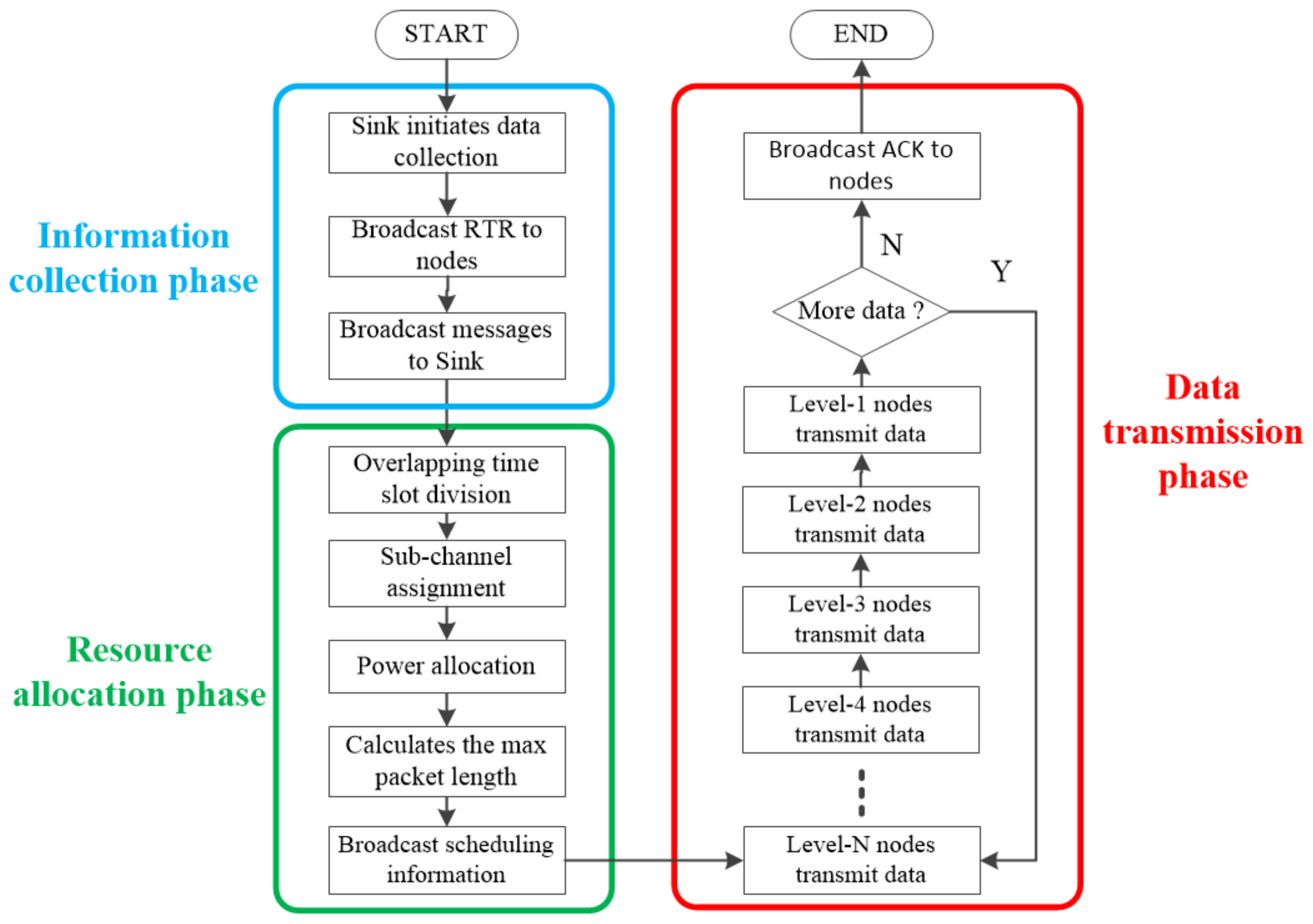
TF-MAC includes three phases: an information collection phase, a resource allocation phase, and a data transmission phase. Figure 2 shows a flowchart for TF-MAC.
In data-collection-oriented UASNs, the data collection activities are initiated by the sink node. When the sink node wants to initiate data collection, it needs to broadcast a request to receive (RTR) packet. The RTR packet serves to wake up the lower layer nodes layer-by-layer. Until the anchor nodes receive the RTR packet, starting from the lowest layer, the nodes with data to be sent will broadcast the information packets to the upper layer. This information packet contains the node ID, node coordinate and node layer number. Then the packets are forwarded layer-by-layer to the sink node.
After the sink node receives the complete information, the network enters the resource allocation phase, which aims to make resource scheduling decisions for each node in the network. First, the overlapping time slot division mechanism is used to assign different slot lengths to the nodes of each layer. Then, a channel and power allocation algorithm is run for each layer respectively, and the subchannel and transmission power are assigned to each individual node of each layer. Finally, to realize the adaptive packet length algorithm based on traffic load in the data transmission phase, the maximum packet length of each node is calculated according to the distance between each node and the expected receiving node. After the sink node has come to a resource scheduling decision, the scheduling information is broadcast to the underwater nodes layer-by-layer. At the end of this phase, each underwater node in the network gets the resource information assigned to it. The length of the phase is not fixed, but it should be long enough to ensure that all underwater nodes get their resource scheduling information.
The data transmission phase is divided into many rounds, each of which consists of overlapping time slots. TDMA between different layer nodes and multi-channel communication between nodes of the same layer are used to avoid vertical and horizontal interference. They enable both vertical and horizontal parallel communication. We consider non-aggregate scheduling for underwater data collection, which means there is no such requirement to decide who always has the priority to transmit first between different layers. Therefore, although the data transmission in Figure 2 is carried out layer-by-layer, the actual situation is not strictly ordered between layers. In the process of data transmission, each node can adjust the length of sending packets according to the adaptive packet length algorithm. If the sink node no longer needs to collect data, an acknowledgment (ACK) packet will be broadcast to the underwater nodes to end the data transmission phase.

4.2. Overlapping Time Slot Division

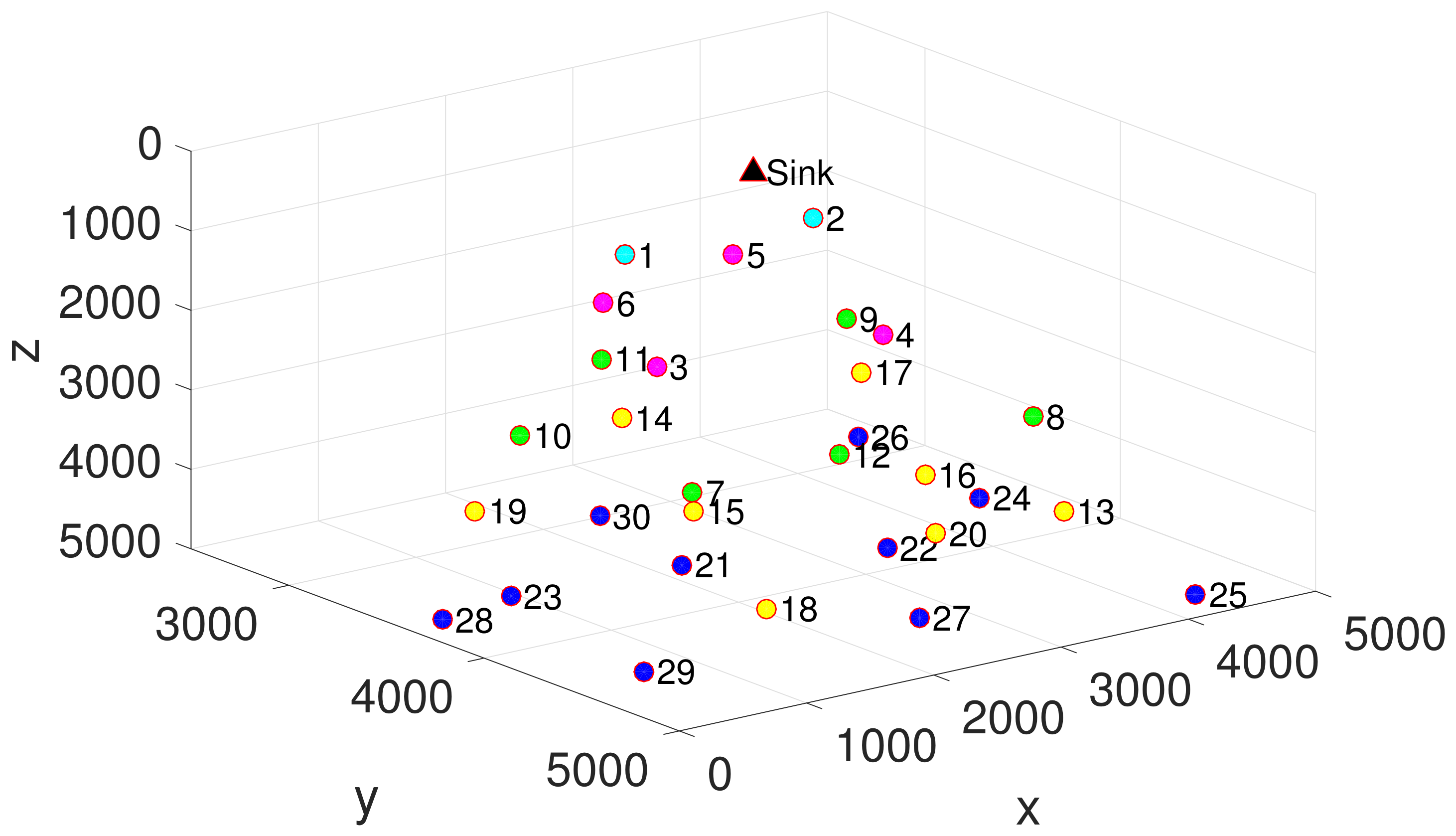
In the network described in Figure 1, the closer to the sea surface, the more data are carried by the underwater node. If a relay node is responsible for forwarding the data from m nodes of the lower layer, then the data size it needs to send in each round can be calculated by Equation (5). Therefore, to improve the fairness of nodes of different depths sending their own data, slots of different lengths are assigned to nodes of different layers. Nodes in the same layer have the same time slot.
v o l s u m = i = 1 m v o l i + v o l s e l f
where v o l i is the data size of node i in the lower layer, with unit of bits. v o l s e l f is the data size generated by the relay node itself.
In TF-MAC, the DATA packet mainly contains the synchronization header, the sending node ID, the destination node ID, the data size, and the data to be transmitted. Figure 3 shows the DATA packet format. In a network with N layers, since the anchor node has no forwarding task, the data size in each packet of the anchor node is v o l N . Then, according to the quantitative relationship of nodes between adjacent layers, the data size is successively allocated to the upper layers. The data size in a single packet of layer—L is calculated by Equation (6). After calculating the data size of each layer, the length of DATA packet can be calculated according to the DATA packet format.
v o l L = n u m L + 1 n u m L · v o l L + 1 + v o l s e l f
where n u m L + 1 / n u m L is the number of layer— L + 1 /layer—L. v o l L + 1 is the data size in the packet of layer— L + 1 .
After determining the packet length T d a t a _ L allocated for each layer, we can calculate the time slot length T s l o t _ L of each layer accordingly. The maximum propagation delay should be taken into account to ensure that the DATA packet is fully received at the destination node [37]. The maximum propagation delay T p r o b is usually calculated by R d / V s , and V s is the speed of sound in water. However, due to the variation in underwater environmental parameters (e.g., temperature, salinity, and pressure) with depth, the distribution of V s is variable [38]. Moreover, there are also affects of the sea waves movements [39] that can cause propagation delays to be variable in different sea layers. Therefore, we need to consider adding protection time slots when performing time slot division. The time slot length of nodes at layer—L can be calculated by Equation (7).
T s l o t _ L = T d a t a _ L + T p r o b + T S I F S
where T S I F S is the length of the short frame protection interval.
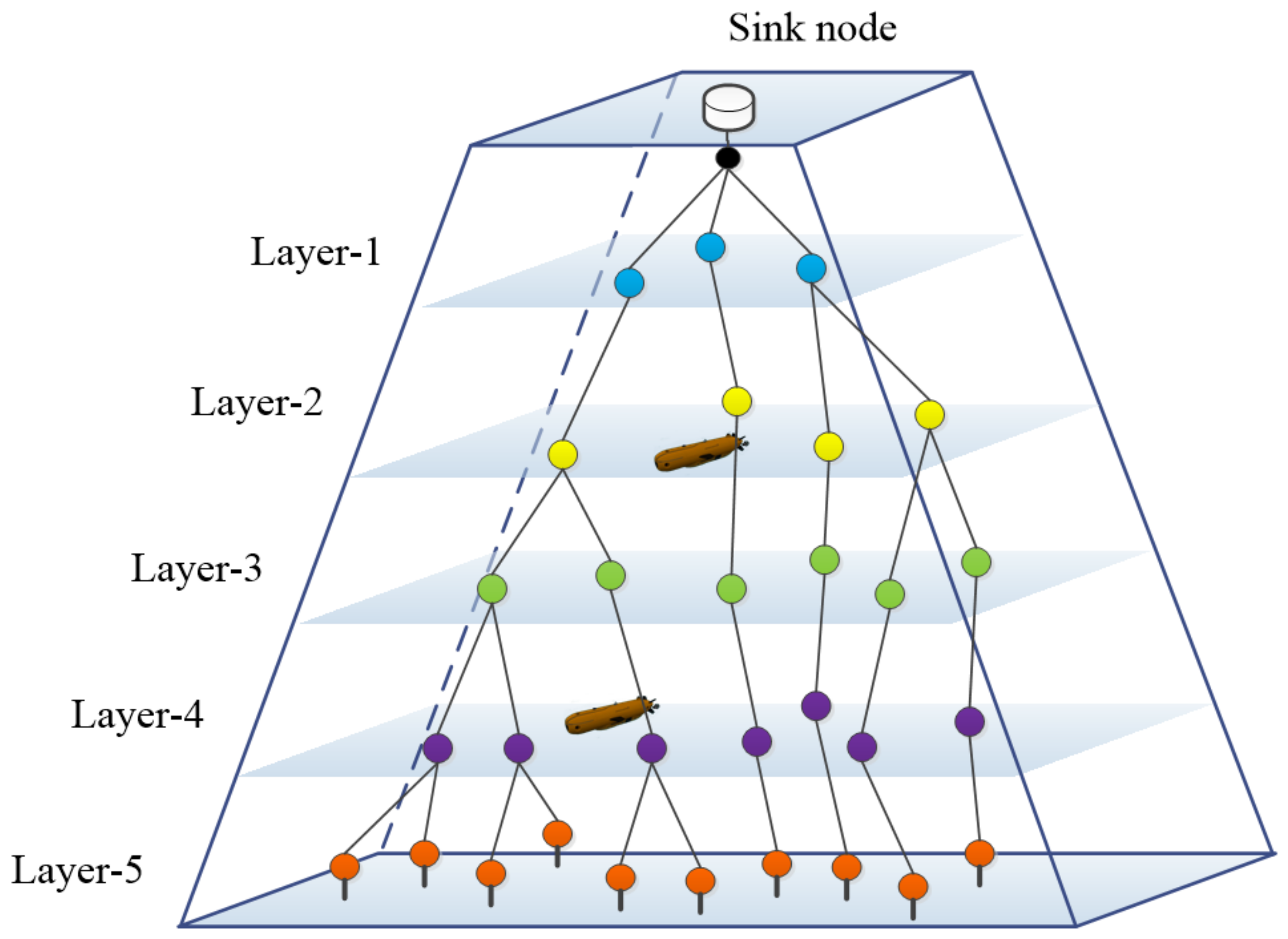
Figure 4 shows a five-hop data collection network, assuming that the transmission path of the entire network is established. We can observe that layers separated by two layers can simultaneously transmit data to nodes in the upper layer without conflict, such as layer-5 and layer-2. Thus, in every round, the time slots of nodes two layers apart can overlap. Figure 5 shows the time slot distribution for each round of the five-hop data collection network in Figure 4. The closer the layer is to the water surface, the longer the time slot. Through overlapping time slot division, the nodes of different levels can communicate in parallel in vertical direction. The throughput is improved and the end-to-end latency is significantly reduced.

4.3. Channel and Power Allocation Algorithm

In this subsection, we design the channel allocation algorithm and power control algorithm of TF-MAC.

4.3.1. Channel Allocation Algorithm

TF-MAC is a multi-channel media access control protocol. The protocol interference model is used to simulate the interference environment. After the information collection phase, the sink node obtains the three-dimensional coordinates of all the underwater nodes in the network. Therefore, the distance between any two nodes can be calculated. The sink node allocates channels layer-by-layer from the anchor nodes upward. To allocate channels for nodes of layer—L, we first construct expected sending node tables for each node of layer— L 1 according to the maximum transmission range. If there is a sending node in the expected sending node tables of multiple nodes of the upper layer, it is kept only in the expected sending node table of the nearest node. The expected sending node tables represent the transmission links of the sending nodes to the upper receiving nodes.
Then, we construct the interference node tables for each node of layer— L 1 according to the interference range in the protocol interference model. The node of layer—L within the maximum interference range of the receiving node is put into the interference node table of the receiving node. By traversing the number of nodes in the interference node tables of the upper receiving nodes, the maximum number of nodes m within a single interference range can be obtained. In order to avoid horizontal collision of data transmission between nodes, we divide the channel into m subchannels with equal bandwidths. In addition, if there is a mobile node in this layer, the channel needs to be divided into m + 1 subchannels, where the mobile node is first allocated to the highest frequency subchannel.
Different nodes in the same layer have different priorities. Because the propagation loss of sound waves is dependent on distance and frequency, the propagation loss at high frequency is more severe than that of low frequency. Therefore, the priority of nodes is sorted according to their distance from the receiving node. The greater the distance from the expected receiving node, the higher the priority of the node. The nodes are allocated subchannels in order of priority from high to low. When allocating a subchannel to a node, the subchannel with the lowest center frequency is selected from the remaining assignable subchannels in the interference node tables to which the node is located.
An example of channel allocation for the nodes of layer-2 is given. Table 1 presents the expected sending node tables and interference node tables constructed for the nodes of layer-1. For visual demonstration, we draw the interference diagram according to Table 1, as shown in Figure 6. The maximum number of nodes within a single interference range is three, and there is a mobile node in layer-2. Therefore, we divide the channel into four subchannels of equal bandwidth, which are CH = SC1, SC2, SC3, SC4 according to the frequency change from low to high. The priority list of the nodes in layer-2 is P = N1, N4, N3, N5, N2, N6. According to the channel allocation algorithm, the node with higher priority is allocated subchannels of lower frequency, and the allocation result is shown in Figure 6. The channel allocation algorithm not only avoids the horizontal conflict of data transmission, but also provides the opportunity of parallel communication within a layer.

4.3.2. Power Control Algorithm

The channel allocation algorithm realizes conflict-free subchannel scheduling based on the protocol interference model. However, unnecessary transmission power can result in a wider interference range and energy waste. Therefore, a power control algorithm based on the physical interference model is designed to ensure the complete non-conflict of multi-channel transmission. Energy consumption is greatly reduced without sacrificing network connectivity.
The sink node runs the power control algorithm in a centralized way to allocate the transmitted power to nodes of each layer. We consider the decoding threshold S I N R t h of the receiving node limited by the physical interference model to determine whether the receiver can receive successfully. Because the energy of the underwater nodes is limited, and to improve the space-reuse efficiency in the network, we minimize the total power sum of each layer. Therefore, the following optimization problem Equation (8) should be solved to ensure that the total energy consumption of the nodes at layer L is minimized.
m i n P s u m _ L = i = 1 n u m L p i S . t . 0 p i p m a x ( 1 i n u m L ) S I N R i = p i · h i N s + j = 1 n i p j h j i S I N R t h ( 1 i n u m L )
where n u m L is the total number of nodes in the layer—L. p i is the power allocated to the ith node in layer—L. p m a x is the maximum transmission power. S I N R i is the S I N R at the expected receiving node of the ith node in the layer—L. n i is the number of interfering nodes that have the same channel as the ith node. h i is the channel gain from the ith node to its intended receiving node. h j i is the channel gain of the interfering node.
The channel allocation algorithm makes interference exist only between nodes that have the same subchannel. We divide the channel into m subchannels at the layer—L; thus, the optimization problem can be divided into m suboptimization problems, which represent the power control between nodes allocated to the same subchannel, respectively. If there are a total of n nodes using SC1 in layer—L, the suboptimization problem of power control of nodes allocated with SC1 can be expressed by Equation (9).
m i n P s u m _ L _ S C 1 = i = 1 n p i S . t 0 p i p m a x ( 1 i n ) S I N R i S I N R t h ( 1 i n )
In the suboptimization problem, the S I N R of each node is related to the transmission power of the other interference nodes. By proof by contradiction, we can find that when the S I N R i S I N R t h term in the constraint is set to be equal, the suboptimization problem obtains the optimal solution. Therefore, the suboptimization problem can be solved by calculating the multivariate first order equations. p i can be solved by Equation (10). By solving the m suboptimization problems, optimization problem Equation (8) is solved.
p i = ( N s + j = 1 n 1 p j h j i ) · S I N R t h / h i
If there is a mobile node in a layer, considering its mobility, we cannot determine with which upper receiving node it will establish a link nor the communication distance. Therefore, the maximum transmission power is allocated on its proprietary subchannel.

4.4. Adaptive Packet Length Algorithm

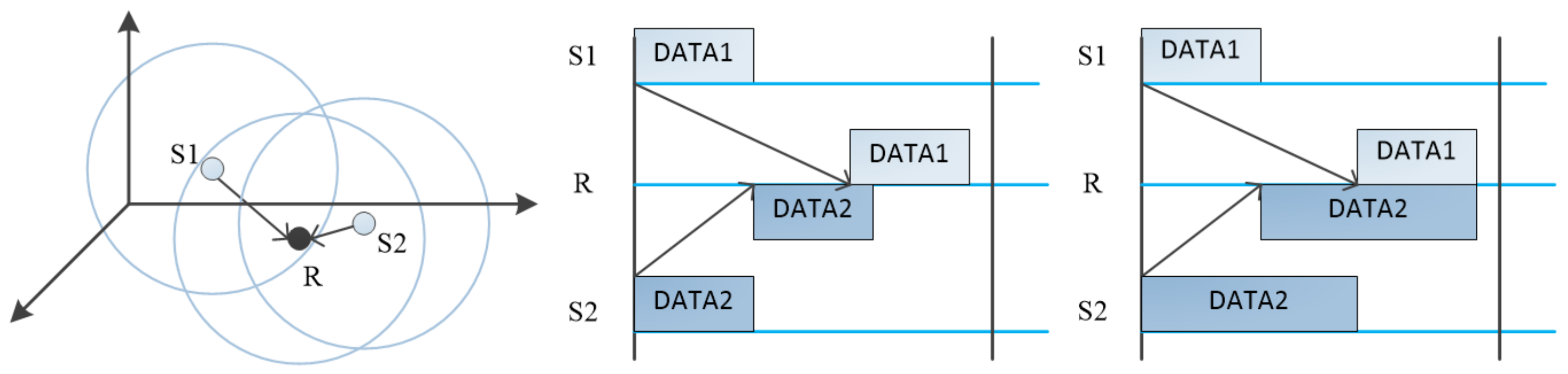
Different from the terrestrial wireless sensor network, the high propagation delay of underwater acoustic channels leads to serious spatial-temporal uncertainty in UASNs. As shown in Figure 7, both sender 1 and sender 2 send packets to the same receiver. Since the distance between them and the receiver is different, their packets do not arrive at the receiver at the same time. In this case, there will be a conflict if sender 1 and sender 2 use the same channel. Since TF-MAC allocates different subchannels to nodes in the same interference range, there will be no packet conflict caused by the spatial-temporal uncertainty at the receiver.
Figure 7 shows that sender 1 and sender 2 send packets at the same time, but because sender 2 is closer to the receiver, it can send longer packets than sender 1 without causing conflicts between time slots. Therefore, considering the distance between the sending node and the expected receiving node and the dynamic of traffic load, we propose an adaptive packet length algorithm.
In the resource allocation phase, the sink node allocates uniform packet length to each layer according to the maximum propagation delay. However, considering the dynamic traffic load of the node, the sending node can adjust the length of the sending packet adaptively within an appropriate range. When the traffic load of the node increases, it adaptively increases the packet length, thus increasing the data size sent in a single time slot. When the traffic load of the node decreases, it adaptively reduces the packet length. However, the packet length of the sender cannot exceed the maximum packet length, which is calculated by Equation (11).
T m a x = T u n i + ( R d d ) / V s
where T u n i is the uniform packet length allocated to node, and d is the distance between the node and the expected receiver.
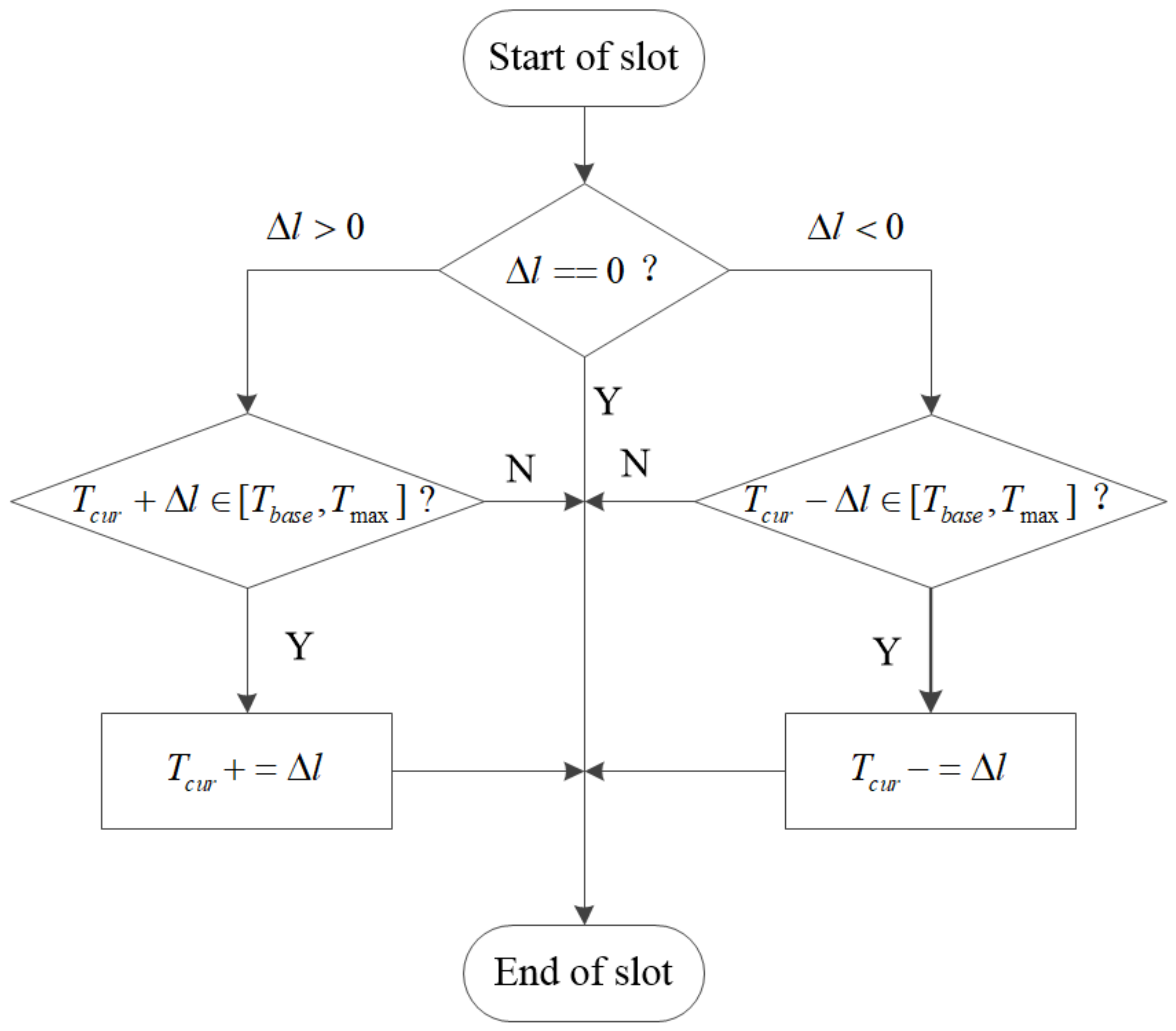
The proposed adaptive packet length algorithm is shown in Figure 8. Each node has a buffer to hold data to be sent, whose size is fixed. If the buffer is full, newly generated data will overflow from the buffer, resulting in loss of data. At this point, increasing the length of the packet can effectively alleviate the loss of data and reduce the packet header overhead. If the traffic load is light, reducing the packet length can send the packet in a timely manner and thus reduce the end-to-end delay. This algorithm is an adaptive packet length algorithm based on a fixed gradient. Δ l represents the fixed gradient, whose absolute value is fixed. Whether the sign of the fixed gradient Δ l is positive or negative is determined by the gradient rise and gradient fall of the traffic load. If the amount of data in the buffer remains unchanged within a certain range, the fixed gradient changes to 0. The packet length T c u r is updated adaptively at the beginning of the time slot. If Δ l > 0 , T c u r will increase; if Δ l < 0 , T c u r will decrease; if Δ l = 0 , T c u r will remain unchanged. The packet length cannot be less than the uniform packet length of the node nor greater than the maximum packet length.
The adaptive packet length algorithm can deal with the time-varying traffic loads of the nodes and improve the adaptability of the MAC protocol; thus, it can be used in many key applications of underwater data collection network.

5. Sea Experiment to Prove the Spatial-Temporal Uncertainty

We evaluate the spatial-temporal uncertainty of UASNs in a sea experiment using our existing underwater acoustic modems [
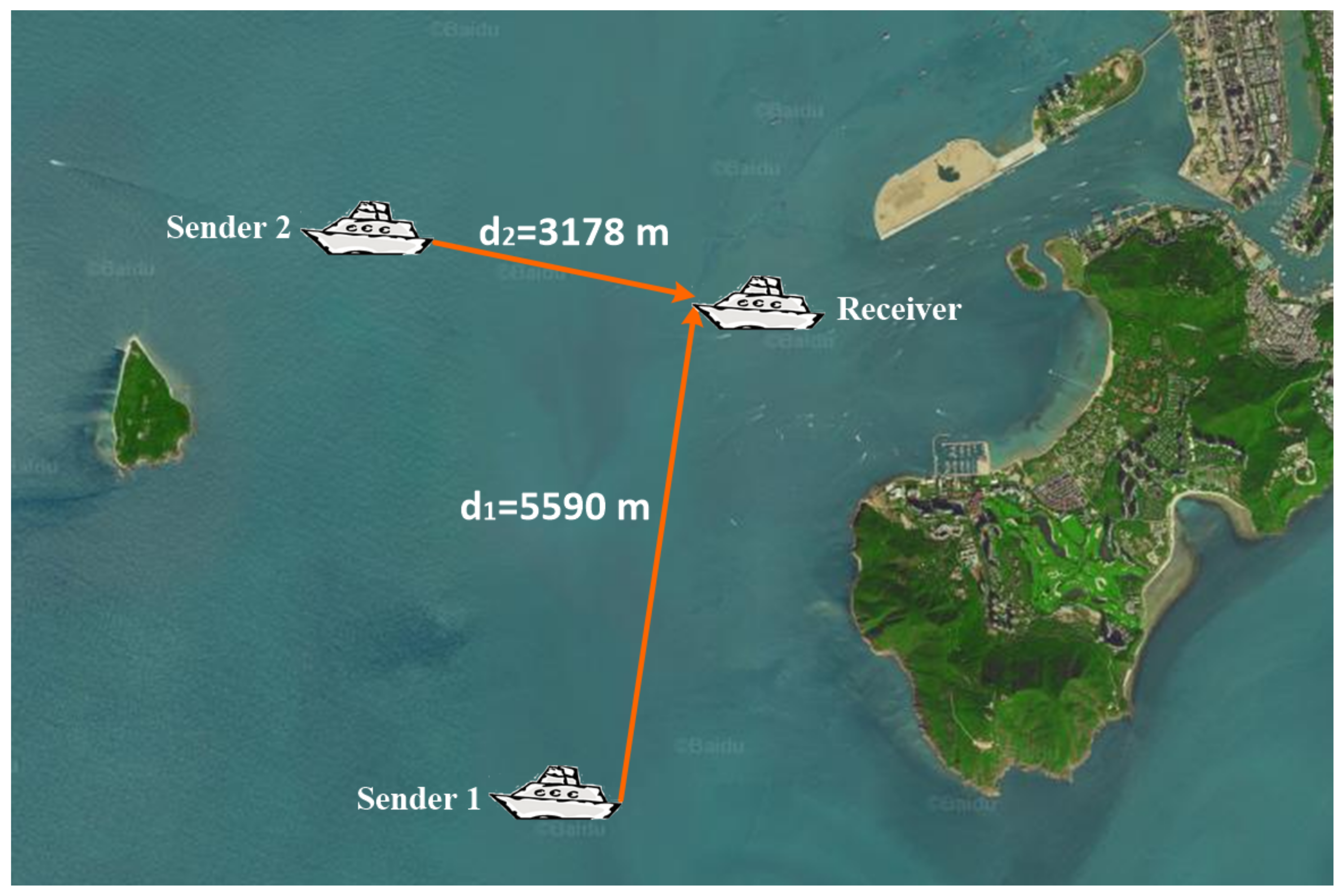
40]. It provides the feasibility for the adaptive packet length algorithm. Our experiment was conducted on 2 December 2020 in Sanya Bay, China. Three ships depart from the dock and anchor at their respective fixed locations, representing two sending nodes and one receiving node. By locating the ships on the map, we create the topology as shown in Figure 9.
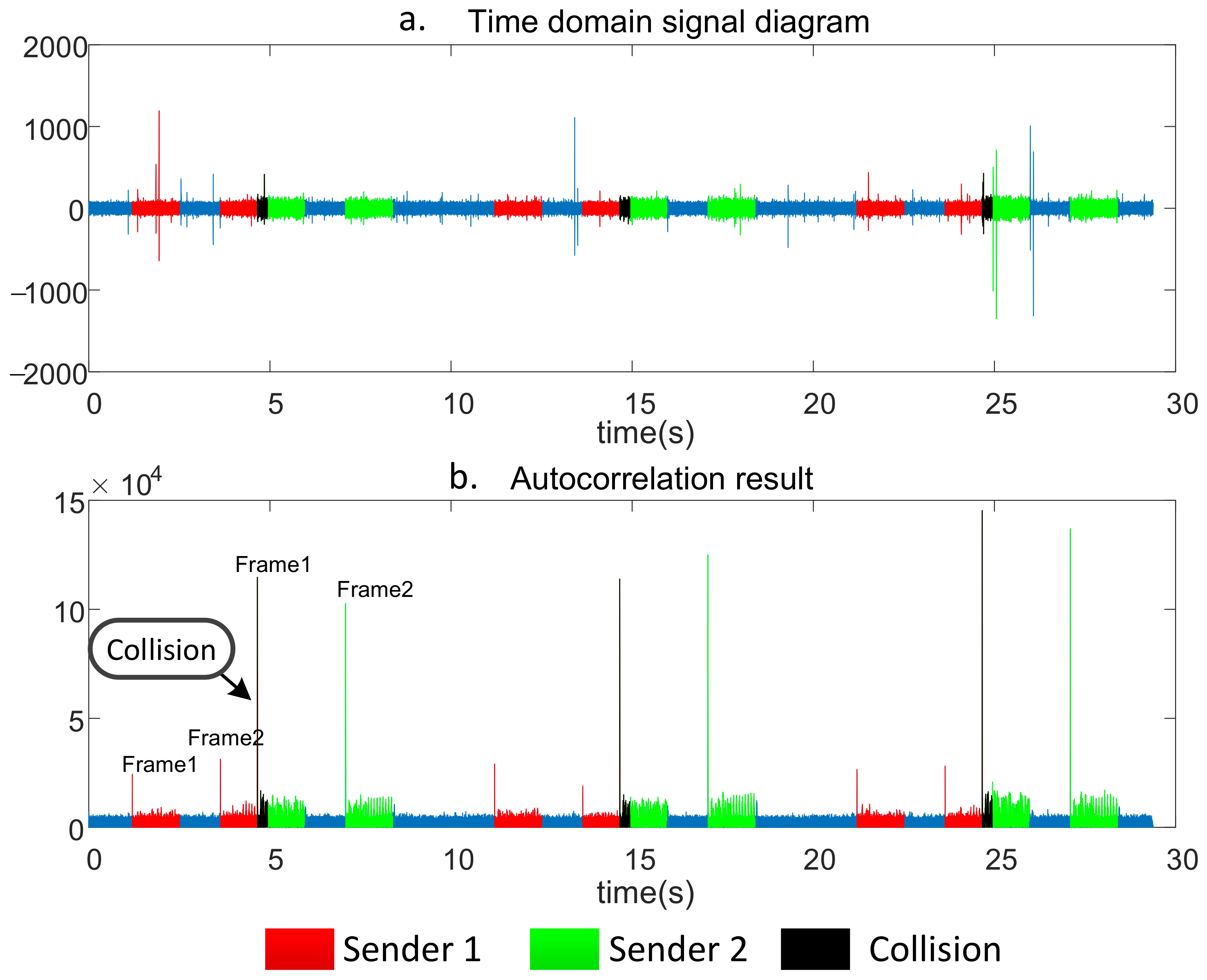
In the experiment, we use the framework of TDMA. Accurate time synchronization is achieved with Ublox GPS’s PPS second pulse. Senders 1 and 2 send packets of fixed length to the receiver. Each node sends two packets at a time, each 1.3 s in length and 1 s apart. The time between the two senders to start sending the first packet is 5 s. Figure 10 shows the signal received by the receiver. Figure 10a is the time domain diagram of the received signal. Figure 10b is the autocorrelation result of synchronous processing. As can be seen from Figure 10, although both sender 1 and sender 2 send packets of the same length at the beginning of the slot, they still collide. The black part shows that the signal from sender 1 and the signal from sender 2 overlap and collide.
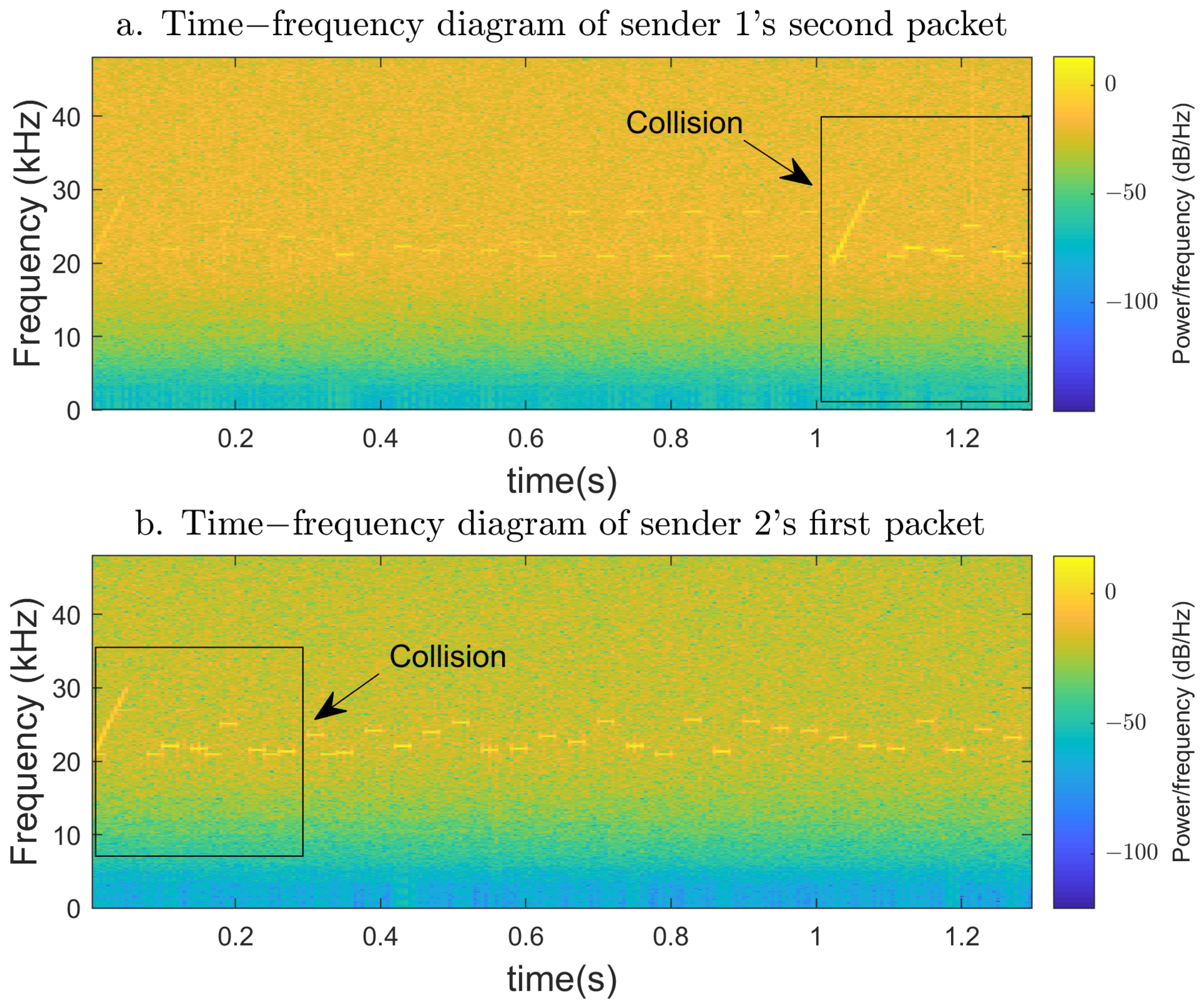
Then we analyze the error code problem caused by the collision at the receiver. As shown in Figure 11a, the time-frequency diagram of the second packet sent by sender 1 for the first time is provided. The synchronization head from sender 2 begins to appear in 1 s of the packet. In addition, the codes that follow are also interfered with by other frequencies. We demodulated the signal and found that the 15th to 20th codes in the packet had errors. Figure 11b provides the time-frequency diagram of the first packet sent by sender 2 for the first time. Although the energy of the signal from sender 2 is stronger than that from sender 1 due to the shorter distance, there is still interference from the signal from sender 1 at the beginning of the signal. However, because sender 2’s signal is more powerful, we found no packet loss due to interference with the synchronization head. After demodulation, the signal of sender 2 has no error due to collision.
Our experimental results show that spatial-temporal uncertainty of UASNs exists, which means the arrival time of packet is not only related to the sending time but also related to the distance between sender and receiver. Ignoring the spatial-temporal uncertainty of the underwater acoustic channel will result in packet collision and code error.

6. Simulation

In this section, we conduct simulations to compare TF-MAC with MC-UWMAC [29] (multi-channel MAC protocol), DBR-MAC [12] and SFAMA [20] (all single-channel protocols).

6.1. Simulation Settings

We implement simulations on Aqua-Sim, an NS-2 based simulator for underwater sensor networks [41]. We deployed a sink node in the center of the 5000 × 5000 m area on the water surface. In the 5000 × 5000 × 5000 m area, 30 or 50 underwater sensor nodes are placed according to the layered network with a tree topology, representing sparse and dense networks, respectively. Sparse topology is shown in Figure 12. Nodes of the same color are on the same layer. Each underwater node generates data following a Poisson process. The data generation rate provided varies from 50 bps to 500 bps. Except for TF-MAC, DATA packets are generated at a fixed size of 200 B. The size of the control packet is 20 B. In our simulation, each run lasts 10,000 s, and we count the average value of twenty runs. The summary of simulation parameters is shown in Table 2.
We measure throughput, delay, average energy consumption and the fairness index as the functions of the data generation rate and number of nodes. Specifically, throughput is the ratio of the number of bits received by the sink node to the simulation time. The delay is the average end-to-end delay of each packet received by the sink. The average energy consumption is calculated by dividing the total network energy consumption by the number of bits successfully received by the sink node. The fairness index indicates the fairness of access to the channel. Here, with the application of Jain’s fairness index [42], the fairness index is defined as Equation (12).
F a i r n e s s I n d e x = ( x i ) 2 N · x i 2
where x i is the number of bits received by the sink node from the node i, 1 < = i < = I , and I is the number of underwater nodes. The value of the fairness index ranges from 0 to 1.

6.2. Simulation Results

6.2.1. Throughput

Figure 13 and Figure 14 show the throughput of the four protocols under the sparse network and the dense network, respectively. Through the contrast results, we can see that the throughput of TF-MAC is higher than DBR-MAC, MC-UWMAC and S-FAMA, especially under the dense network. This is because TF-MAC’s overlapping time slot division and multi-channel mechanism enables both vertical and horizontal parallel communication, which greatly improve channel utilization. Although the multi-channel mechanism is also adopted by MC-UWMAC, it does not consider the problem of imbalanced traffic load among nodes of different depths. Moreover, with the increase in node density, the number of subchannels will increase exponentially, exceeding the increase in the number of nodes. Therefore, the higher node density does not result in a significant throughput increase in MC-UWMAC compared to the other three protocols.
Regardless of the network density, the throughput of the four protocols all reach a saturation state with the increase in data generation rate. When the sparse network reaches saturation, the throughput of TF-MAC is 15.7% higher than DBR-MAC, 114.6% higher than MC-UWMAC and 146.6% higher than SFAMA. When the dense network reaches saturation, the throughput of TF-MAC is 25.1% higher than DBR-MAC, 143.1% higher than MC-UWMAC, and 158.8% higher than SFAMA. The throughputs of TF-MAC and DBR-MAC are significantly higher than MC-UWMAC and SFAMA because they consider the application scenario of data collection networks. They all introduce a depth-based scheme and set different access channel priorities for nodes of different depths. In DBR-MAC, high RTS collision occurs when the data generation rate exceeds the available capacity. In TF-MAC, nodes access the channel based on the scheduled time, which realizes collision-free data transmission. In addition, TF-MAC allows different nodes of the same layer to transmit to the same receiving node without conflict. SFAMA requires several full round-trip exchanges of control packets before each DATA packet is sent, which results in low throughput and low channel utilization. Different from the same-length time slot of SFAMA, TF-MAC divides time slots of different lengths for nodes of different depths to solve the problem of imbalanced network traffic load.

6.2.2. End-to-End Delay

Figure 15 and Figure 16 show that delay of TF-MAC is smaller than those of the other three protocols in both the sparse and dense networks. Especially in the sparse network, TF-MAC can reduce end-to-end delay by at least 34.2%. This is because TF-MAC takes into account the depth-based load imbalance in the data collection network. It sets different slot lengths for nodes of different depths to reduce the long queuing delay caused by time-out forwarding. In addition, the adaptive packet length algorithm of TF-MAC also plays a role in reducing delay. As the data generation rate increases, the delay of all four protocols increases.
For SFAMA, as the data generation rate increases, more RTS collisions occur leading to longer delay. In DBR-MAC, when data generation rate increases, data flow may become congested at critical nodes. To prevent congestion, it introduces a conservative backoff algorithm, which increases the delay performance gap between DBR-MAC and TF-MAC. For MC-UWMAC, the control channel adopts the time-slot method; thus, the node can only send RTS in its own time slot. In addition, the smaller data channel bandwidth increases the transmission time in MC-UWMAC. In TF-MAC, DATA packets are transmitted without conflict. Initially, the network does not reach saturation; thus, the delay is basically unchanged in TF-MAC. As the data generation rate increases further, the buffer becomes full; thus, the delay of all four MAC protocols will flatten out.
Comparing the results in Figure 15 and Figure 16, the delay of all protocols except DBR-MAC becomes larger as the node density increases. This difference is because in DBR-MAC, the number of candidate forwarders is larger in dense network; thus, it has a higher probability of having an optimal next hop. In SFAMA, the probability of RTS collision caused by the dense network is higher. For TF-MAC and MC-UWMAC, the dense network increases the length of the time slot, which increases the average end-to-end delay.

6.2.3. Average Energy Consumption

Figure 17 and Figure 18 show that the average energy consumption of TF-MAC is lower than those of the other three protocols under the same data generation rate. This difference is mainly due to the power control algorithm for the nodes at each layer in the TF-MAC. Underwater nodes use optimized transmission power, which not only saves energy but also avoids unnecessary interference. In contrast, the other three protocols use a fixed amount of transmitting power to forward packets to the sink node. Second, the adaptive packet length algorithm in TF-MAC enables the node to increase the data size sent in a single slot when the traffic load increases, which further reduces energy consumption caused by the packet header. In MC-UWMAC, the small data channel bandwidth increases the transmission time, which results in greater energy consumption.
By comparing the results of Figure 17 and Figure 18, the average energy consumption of all protocols becomes larger with an increase in node density. SFAMA and DBR-MAC are two contention-based protocols, and the probability of RTS collision is more prominent in the dense network, thus wasting a lot of energy. For the two multi-channel protocols, TF-MAC and MC-UWMAC, an increase in node density causes the bandwidth of the subchannel allocated to each node becomes smaller, which further increases the transmission time. However, compared with MC-UWMAC, the subchannel bandwidth of TF-MAC decreases less. Therefore, the energy consumption increase of TF-MAC from the sparse network to the dense network is smaller. Specifically, when the data generation rate is 50 bps, the energy consumption of TF-MAC increases by 56.8%, while that of MC-UWMAC increases by 77.6%.

6.2.4. Fairness Index

In data-collection-oriented UASNs, the underwater nodes from different depths have to generate their own data. Deeper nodes require more hops to forward data to the sink node. Shallower nodes transmit their own data as well as forward data from deeper nodes. Therefore, it is very important to help the nodes at different depths achieve fairness in transmitting their own data to the sink node.
Figure 19 and Figure 20 show that TF-MAC has the highest fairness index. Moreover, since TF-MAC and DBR-MAC both consider the application of the data collection network, their fairness is obviously higher than that of MC-UWMAC and SFAMA. Overlapping time slot division scheme in TF-MAC enables the nodes in the upper layer to have longer time slots, allowing larger packet to be sent. The DATA packet contains not only the data from the sending node itself but also the data from the lower layers. This means that nodes of different depths have the same priority to transmit data to the sink. DBR-MAC selects the optimal forwarding node for the deeper nodes to improve their chances of transmitting data to the sink node. However, depth-based backoff algorithms greedily give priority to key nodes to maximize performance, which reduces fairness. As the data generation rate exceeds the available capacity, the backoff algorithm changes from a depth-based algorithm to a conservative algorithm, thus the fairness index increases.
By comparing Figure 19 and Figure 20, the fairness indices of the four protocols all decrease with an increase in node density. The more severe node distribution inhomogeneity in dense network makes the fairness index of TF-MAC decrease. However, the fairness index of TF-MAC decreases the least. When the data generation rate is 100 bps, the fairness index of TF-MAC under dense network is decreased by 2.1% compared with the sparse network.
Figure 21 shows the fairness indices of different layers in TF-MAC under the sparse network. Different layers have different fairness due to the uneven distribution of nodes, but they are all greater than 0.8. In addition, the fairness index in each layer decreases with an increase in the data generation rate.

7. Conclusions

In this paper, we consider the application of underwater data collection and find that directional packet transmissions lead to traffic load imbalance. Motivated by this problem, we propose a traffic-aware fair MAC protocol for layered data-collection-oriented UASNs, called TF-MAC. To eliminate the possibility of conflict, a TDMA mechanism is used between layers, and a multi-channel mechanism and channel and power allocation algorithm are used in the same layer. An overlapping time slot division scheme allocates time slots of different lengths to different layers and enables parallel communication among different layers. Considering the time-varying traffic loads of the nodes, an adaptive packet length algorithm is introduced. Our sea experiment verifies the existence of underwater spatial-temporal uncertainty, which provides a feasible basis for the adaptive packet length algorithm. Simulation results show that the proposed TF-MAC achieves good performance in the data-collection-oriented UASNs.
In future work, we will focus on the feasibility and adaptability of TF-MAC in dynamic networks.

Author Contributions

Conceptualization, S.Y.; methodology, S.Y.; software, X.L.; validation, S.Y. and X.L.; formal analysis, S.Y.; investigation, S.Y. and X.L.; resources, Y.S.; data curation, S.Y.; writing—original draft preparation, S.Y.; writing—review and editing, X.L.; visualization, S.Y. and X.L.; supervision, Y.S.; project administration, X.L.; funding acquisition, Y.S. All authors have read and agreed to the published version of the manuscript.

Funding

This research was funded by the National Natural Science Foundation of China under Grant 62171310.

Institutional Review Board Statement

Not applicable.

Informed Consent Statement

Not applicable.

Data Availability Statement

The data presented in this paper are available after contacting the corresponding author.

Conflicts of Interest

The authors declare no conflict of interest.

References

  1. Murad, M.; Sheikh, A.A.; Manzoor, M.A.; Felemban, E.; Qaisar, S. A survey on current underwater acoustic sensor network applications. Int. J. Comput. Theory Eng. 2015, 7, 51–56. [Google Scholar] [CrossRef] [Green Version]
  2. Songzuo, L.; Iqbal, B.; Khan, I.; Ahmed, N.; Qiao, G. Full Duplex Physical and MAC Layer-Based Underwater Wireless Communication Systems and Protocols: Opportunities, Challenges, and Future Directions. J. Mar. Sci. Eng. 2021, 9, 468. [Google Scholar] [CrossRef]
  3. Felemban, E.; Shaikh, F.K.; Qureshi, U.M.; Sheikh, A.A.; Qaisar, S.B. Underwater sensor network applications: A comprehensive survey. Int. J. Distrib. Sens. Netw. 2015, 11, 896832. [Google Scholar] [CrossRef] [Green Version]
  4. Hu, Y.; Wang, D.; Li, J.; Wang, Y.; Shen, H. Adaptive Environmental Sampling for Underwater Vehicles Based on Ant Colony Optimization Algorithm. In Proceedings of the Global Oceans, Biloxi, MS, USA, 5–30 October 2020; US Gulf Coast: Singapore, 2020; pp. 1–9. [Google Scholar]
  5. Sun, Z.; Guo, H.; Akyildiz, I.F. High-Data-Rate Long-Range Underwater Communications via Acoustic Reconfigurable Intelligent Surfaces. IEEE Commun. Mag. 2022, 60, 96–102. [Google Scholar] [CrossRef]
  6. Jiang, S. On securing underwater acoustic networks: A survey. IEEE Commun. Surv. Tutor. 2018, 21, 729–752. [Google Scholar] [CrossRef]
  7. Wu, X.; Hu, F.; Zou, P.; Chi, N. Application of Gaussian Mixture Model to Solve Inter-Symbol Interference in PAM8 Underwater Visible Light System Communication. IEEE Photonics J. 2019, 11, 1–10. [Google Scholar] [CrossRef]
  8. Su, Y.; Xu, Y.; Pang, Z.; Kang, Y.; Fan, R. HCAR: A Hybrid Coding-Aware Routing Protocol for Underwater Acoustic Sensor Networks. IEEE Internet Things J. 2023; Early Access. [Google Scholar] [CrossRef]
  9. Chen, Y.J.; Wang, H.L. Ordered CSMA: A collision-free MAC protocol for underwater acoustic networks. In Proceedings of the OCEANS 2007, Vancouver, BC, Canada, 29 September–4 October 2007; pp. 1–6. [Google Scholar]
  10. Hong, L.; Hong, F.; Guo, Z.W.; Yang, X. A TDMA-based MAC protocol in underwater sensor networks. In Proceedings of the 2008 4th International Conference on Wireless Communications, Networking and Mobile Computing, Dalian, China, 12–14 October 2008; pp. 1–4. [Google Scholar]
  11. Zhang, J.; Cai, M.; Han, G.; Qian, Y.; Shu, L. Cellular clustering-based interference-aware data transmission protocol for underwater acoustic sensor networks. IEEE Trans. Veh. Technol. 2020, 69, 3217–3230. [Google Scholar] [CrossRef]
  12. Li, C.; Xu, Y.; Diao, B.; Wang, Q.; An, Z. DBR-MAC: A depth-based routing aware MAC protocol for data collection in underwater acoustic sensor networks. IEEE Sens. J. 2016, 16, 3904–3913. [Google Scholar] [CrossRef]
  13. Zhu, M.; Zhang, W.; Jin, N.; Qin, Z.; Xin, J.; Wang, L. UPMAC: A localized load-adaptive MAC protocol for underwater acoustic networks. IEEE Sens. J. 2015, 16, 4110–4118. [Google Scholar] [CrossRef]
  14. Yin, X.; Zhou, X.; Huang, R.; Fang, Y.; Li, S. A Fairness-Aware Congestion Control Scheme in Wireless Sensor Networks. IEEE Trans. Veh. Technol. 2009, 58, 5225–5234. [Google Scholar] [CrossRef] [Green Version]
  15. Grover, A.; Mohan Kumar, R.; Angurala, M.; Singh, M.; Sheetal, A.; Maheswar, R. Rate Aware Congestion Control Mechanism for Wireless Sensor Networks. Alex. Eng. J. 2022, 61, 4765–4777. [Google Scholar] [CrossRef]
  16. Al Guqhaiman, A.; Akanbi, O.; Aljaedi, A.; Chow, C.E. A Survey on MAC Protocol Approaches for Underwater Wireless Sensor Networks. IEEE Sens. J. 2020, 21, 3916–3932. [Google Scholar] [CrossRef]
  17. Koseoglu, M.; Karasan, E.; Chen, L. Cross-layer energy minimization for underwater ALOHA networks. IEEE Syst. J. 2015, 11, 551–561. [Google Scholar] [CrossRef]
  18. Syed, A.A.; Ye, W.; Heidemann, J.; Krishnamachari, B. Understanding spatio-temporal uncertainty in medium access with ALOHA protocols. In Proceedings of the 2nd Workshop Underwater Networks, Montreal, QC, Canada, 14 September 2007; pp. 41–48. [Google Scholar]
  19. Han, Y.; Fei, Y. DAP-MAC: A delay-aware probability-based MAC protocol for underwater acoustic sensor networks. Ad Hoc Netw. 2016, 48, 80–92. [Google Scholar] [CrossRef] [Green Version]
  20. Molins, M.; Stojanovic, M. Slotted FAMA: A MAC protocol for underwater acoustic networks. In Proceedings of the OCEANS 2006, Asia Pacific, Singapore, 16–19 May 2006; pp. 1–7. [Google Scholar]
  21. Han, S.; Noh, Y.; Lee, U.; Gerla, M. M-FAMA: A multi-session MAC protocol for reliable underwater acoustic streams. In Proceedings of the 32nd IEEE International Conference on Computer Communications, Turin, Italy, 14–19 April 2013; pp. 665–673. [Google Scholar]
  22. Alfouzan, F.A.; Shahrabi, A.; Ghoreyshi, S.M.; Boutaleb, T. A collision-free graph coloring MAC protocol for underwater sensor networks. IEEE Access 2019, 7, 39862–39878. [Google Scholar] [CrossRef]
  23. Alfouzan, F.; Shahrabi, A.; Ghoreyshi, S.M.; Boutaleb, T. An efficient scalable scheduling MAC protocol for underwater sensor networks. Sensors 2018, 18, 2806. [Google Scholar] [CrossRef] [Green Version]
  24. Zhang, R.; Cheng, X.; Cheng, X.; Yang, L. Interference-free graph based TDMA protocol for underwater acoustic sensor networks. IEEE Trans. Veh. Technol. 2017, 67, 4008–4019. [Google Scholar] [CrossRef]
  25. Hsu, C.C.; Lai, K.F.; Chou, C.F.; Lin, K.J. ST-MAC: Spatial-temporal MAC scheduling for underwater sensor networks. In Proceedings of the IEEE INFOCOM, Rio de Janeiro, Brazil, 19–25 April 2009; pp. 1827–1835. [Google Scholar]
  26. Chao, C.M.; Wang, Y.Z.; Lu, M.W. Multiple-rendezvous multichannel MAC protocol design for underwater sensor networks. IEEE Trans. Syst. Man Cybern. Syst. 2012, 43, 128–138. [Google Scholar] [CrossRef]
  27. Zhou, Z.; Peng, Z.; Cui, J.H.; Jiang, Z. Handling Triple Hidden Terminal Problems for Multichannel MAC in Long-Delay Underwater Sensor Networks. IEEE Trans. Mob. Comput. 2012, 11, 139–154. [Google Scholar] [CrossRef]
  28. Yang, M.; Gao, M.; Foh, C.H.; Cai, J. Hybrid collision-free medium access (HCFMA) protocol for underwater acoustic networks: Design and performance evaluation. IEEE J. Ocean. Eng. 2014, 40, 292–302. [Google Scholar] [CrossRef]
  29. Bouabdallah, F.; Zidi, C.; Boutaba, R.; Mehaoua, A. Collision avoidance energy efficient multi-channel MAC protocol for underwater acoustic sensor networks. IEEE Trans. Mob. Comput. 2018, 18, 2298–2314. [Google Scholar] [CrossRef]
  30. Kredo II, K.; Djukic, P.; Mohapatra, P. STUMP: Exploiting position diversity in the staggered TDMA underwater MAC protocol. In Proceedings of the IEEE INFOCOM, Rio de Janeiro, Brazil, 19–25 April 2009; pp. 2961–2965. [Google Scholar]
  31. Deng, M.; Chen, H.; Xie, L. A hybrid MAC protocol in data-collection-oriented underwater acoustic sensor networks. In Proceedings of the OCEANS, Aberdeen, UK, 19–22 June 2017; pp. 1–7. [Google Scholar]
  32. Yang, M.; Gao, M.; Foh, C.H.; Cai, J.; Chatzimisios, P. DC-MAC: A data-centric multi-hop MAC protocol for underwater acoustic sensor networks. In Proceedings of the IEEE Symposium on Computers and Communications (ISCC), Kerkyra, Greece, 28 June–1 July 2011; pp. 491–496. [Google Scholar]
  33. Su, Y.; Guo, L.; Jin, Z.; Fu, X. A Mobile-Beacon-Based Iterative Localization Mechanism in Large-Scale Underwater Acoustic Sensor Networks. IEEE Internet Things J. 2021, 8, 3653–3664. [Google Scholar] [CrossRef]
  34. Wang, S.; Wang, Y.; Guan, X. An interference-free scheduling for the TDMA protocol in multi-hop underwater acoustic grid networks. In Proceedings of the OCEANS 2017, Anchorage, AK, USA, 18–21 September 2017; pp. 1–5. [Google Scholar]
  35. Zhong, X.; Ji, F.; Chen, F.; Guan, Q.; Yu, H. A New Acoustic Channel Interference Model for 3-D Underwater Acoustic Sensor Networks and Throughput Analysis. IEEE Internet Things J. 2020, 7, 9930–9942. [Google Scholar] [CrossRef]
  36. Lu, S.; Wang, Z.; Wang, Z.; Zhou, S. Throughput of underwater wireless ad hoc networks with random access: A physical layer perspective. IEEE Trans. Wirel. Commun. 2015, 14, 6257–6268. [Google Scholar] [CrossRef]
  37. Zheng, H.; Wu, J. Data Collection and Event Detection in the Deep Sea with Delay Minimization. In Proceedings of the 2015 12th Annual IEEE International Conference on Sensing, Communication, and Networking (SECON), Seattle, WA, USA, 22–25 June 2015; IEEE: Piscatawaj, NJ, USA, 2015; pp. 354–362. [Google Scholar]
  38. Chen, C.; Yang, K.; Ma, Y. Sensitivity of Sound Speed Fluctuation on Acoustic Arrival Delay of Middle Range in Deep Water. Appl. Acoust. 2019, 149, 68–73. [Google Scholar] [CrossRef]
  39. Jimenez-Martinez, M. Harbor and Coastal Structures: A Review of Mechanical Fatigue under Random Wave Loading. Heliyon 2021, 7, e08241. [Google Scholar] [CrossRef]
  40. Su, Y.; Dong, L.; Zhou, Z.; Liu, X.; Wei, X. An general embedded underwater acoustic communication system based on advance STM32. IEEE Embed. Syst. Lett. 2020, 13, 90–93. [Google Scholar] [CrossRef]
  41. Xie, P.; Zhou, Z.; Peng, Z.; Yan, H.; Hu, T.; Cui, J.H.; Shi, Z.; Fei, Y.; Zhou, S. Aqua-Sim: An NS-2 based simulator for underwater sensor networks. In Proceedings of the OCEANS, Biloxi, MS, USA, 26–29 October 2009; pp. 1–7. [Google Scholar]
  42. Guo, C.; Sheng, M.; Wang, X.; Zhang, Y. Throughput maximization with short-term and long-term Jain’s index constraints in downlink OFDMA systems. IEEE Trans. Commun. 2014, 62, 1503–1517. [Google Scholar] [CrossRef]
Figure 1. Network model of TF-MAC.
Remotesensing 15 01501 g001
Figure 2. Flowchart of TF-MAC.
Remotesensing 15 01501 g002
Figure 3. DATA packet format.
Remotesensing 15 01501 g003
Figure 4. Five-hop data collection network connection diagram.
Remotesensing 15 01501 g004
Figure 5. Overlapped slot division of a five-hop data collection network in TF-MAC.
Remotesensing 15 01501 g005
Figure 6. Interference diagram of channel allocation for the second layer nodes.
Remotesensing 15 01501 g006
Figure 7. The effect of spatial-temporal uncertainty on packet length nodes.
Remotesensing 15 01501 g007
Figure 8. Flow chart of adaptive packet length algorithm.
Remotesensing 15 01501 g008
Figure 9. Network topology of sea experiment.
Remotesensing 15 01501 g009
Figure 10. The signal received by the receiver.
Remotesensing 15 01501 g010
Figure 11. Time–frequency diagram of packets.
Remotesensing 15 01501 g011
Figure 12. Sparse topology of 30 underwater transmission nodes.
Remotesensing 15 01501 g012
Figure 13. Comparison of throughput in the sparse network.
Remotesensing 15 01501 g013
Figure 14. Comparison of throughput in the dense network.
Remotesensing 15 01501 g014
Figure 15. Comparison of end-to-end delay in the sparse network.
Remotesensing 15 01501 g015
Figure 16. Comparison of end-to-end delay in the dense network.
Remotesensing 15 01501 g016
Figure 17. Comparison of energy consumption per bit in the sparse network.
Remotesensing 15 01501 g017
Figure 18. Comparison of energy consumption per bit in the dense network.
Remotesensing 15 01501 g018
Figure 19. Comparison of the fairness index in the sparse network.
Remotesensing 15 01501 g019
Figure 20. Comparison of the fairness index in the dense network.
Remotesensing 15 01501 g020
Figure 21. Comparison of fairness index at different layers in sparse network.
Remotesensing 15 01501 g021
Table 1. Expected sending node table and interference node table of the first layer nodes.
Layer-1 NodeExpected Sending Node TableInterference Node Table
R1N1, N2, N3N1, N2, N3
R2N3, N4N2, N3, N4
R3N5, N6N5, N6
Table 2. Simulation parameters.
ParameterValue
Transmission range1500 m
Interference range1800 m
Simulation time10,000
Total bandwidth20 kHz (20–40 kHz)
Number of underwater nodes30/50
Transmitting power2 W
Receiving power100 mW
Noise density N s 0.01 W/Hz
Disclaimer/Publisher’s Note: The statements, opinions and data contained in all publications are solely those of the individual author(s) and contributor(s) and not of MDPI and/or the editor(s). MDPI and/or the editor(s) disclaim responsibility for any injury to people or property resulting from any ideas, methods, instructions or products referred to in the content.

